1

Chaos and High Power RF Effects: Statistical Analysis of Induced Voltages

Steven M. Anlage, Sameer Hemmady,Xing Zheng, James Hart, Tom Antonsen, Ed Ott

Research funded by the AFOSR-MURI and DURIP programs

AFOSR Presentation

2

GoalTo develop a quantitative statistical understanding of induced voltage

and current distributions in circuits inside complicated enclosures, based upon minimal information about the system

3

Electromagnetic Compatibility of Circuits

Cables

Cooling Vents

Integrated Ckts

PCB Tracks

Connectors

Ckt Boards

Coupling of external radiation to computer chips is a complex process:

Apertures

Resonant cavities

Transmission Lines

Circuit Elements

System Size > Wavelength

HPM Effects:

Chaotic RayTrajectories

Statistical Distribution using Wave Chaos

We want to understand the scattering propertiesof this system including the effects of coupling

4

Why Quantum / Wave Chaos?

Difficulty in making predictions of electromagneticfield structure in complicated enclosures

Predictions can depend sensitively on details

The “soda can problem”

Related work: (Field distributions in reverberation chambers, etc.)R. Holland and R. St. John, Statistical Electromagnetics (Taylor and Francis,

Philadelphia, 1999).D. A. Hill et al., IEEE Transactions on Electromagnetic Compatibility 36, 169 (1994).L. K. Warne et al., IEEE Trans. Antennas Propag. 51, 978 (2003).and others…

5

The Difficulty in Making Predictions…

8.7 8.8 8.9 9.0 9.1 9.2 9.3

200

400

600

800

1000

Abs

[Zca

v]

Frequency [GHz]8.7 8.8 8.9 9.0 9.1 9.2 9.3

200

400

600

800

1000

Abs

[Zca

v]

Frequency [GHz]

Perturbation Position 1

Perturbation Position 2

Antenna Port

• The EM Response of Complicated Enclosures is Very Sensitive to details (boundary conditions, cable locations, etc.) ⇒ Analytic Solutions are Impractical

• Solution : Statistical Description using Wave Chaos !!

6

¼¼--BowBow--Tie Resonator Tie Resonator EXPERIMENTAL SETUP:EXPERIMENTAL SETUP:

21.6 cm

43.2 cm

54.4 cm

8 mm DEEP

Antenna Entry Points

SCANNED PERTURBATIONS

Circular Arc

R=107 cmR=107 cm

• 2 Dimensional Quarter Bow Tie Wave Chaotic cavity• Classical ray trajectories are chaotic - short wavelength - Quantum Chaos• 1-port, 2-port S and Z measurements in the 3-18 GHz range• Ensemble average through 100 locations and orientations of the perturbations• Perturbers are of size ~λ or bigger

Eigen mode Image at 12.57GHz

Circular Arc

R=63.5 cmR=63.5 cm

Bow-tiebilliard8 mm

4.67 cm

6.06 cm

Perturbation

7

24 ′′=r

5.25 ′′=r

0 4 8 12 16

8

4

0

8

4

00 4 8 12 16

x (inches)

y (in

ches

)

181512840

A2||Ψ

Ferrite

a)

b)

13.69 GHz

13.62 GHz

Wave Chaotic Eigenfunctions

D. H. Wu and S. M. Anlage, Phys. Rev. Lett. 81, 2890 (1998).

Uncover simple statistical properties of:

Eigen-frequencies,Eigen-functions,Scattering matrix,Impedance matrix,Admittance matrix,etc.

Many of these simplestatistical properties aredescribed by RandomMatrix Theory

8

UniversalProperties

Coupling

Statistical EM Responseof real enclosures

Practical Implications for Real Life ProblemsBare Minimum Specifications for Induced-Voltage Statistics

Detail-Independent

What are the bare minimum specifications to accurately predict voltage Statistics?

Frequency, Volume and Losses

Radiation impedance of the ports

Minimum Information: Determine the “Key Parameter”

Determines the shape and scales of cavity Z and S PDFs.

Qkk

n ⋅Δ 2

2

9

Algorithm for Predicting Component Induced-Voltage Distributions:

Qf

V

Frequency

Losses Volume

Universal Impedance z

Cavity Impedance Z

]Re[]Im[ radrad ZzZjZ ⋅+=

Radiation Impedance

radZ

Specific Input Waveform

Mode of HPM Attack

Probability Density Function of Voltages on all components inside enclosure

10

0.0 0.5 1.00

1

2

3

P{|S

|2 }

|S|2

Prescription to Engineer Cavities with Desired Electromagnetic Properties: Simple 1-Port Example

radradcav RzjXZ ⋅+=

-3 -2 -1 0 1 2 30.0

0.3

0.6

P{φ S}

φS

• Freq : 6 to 9.6 GHz

• Antenna Dia (2a)= 1.27mm

radradrad jXRZ +=

Height (h)

CAVITY BASECAVITY BASE

CAVITY LIDCAVITY LID

Radius (a)

CoaxialCable

0.0 0.5 1.00

1

2

3

P{|S

|2 }

|S|2-3 -2 -1 0 1 2 3

0.0

0.3

0.6

P{φ S}

φS

sjeSS φ||=

Numerically Generated (z)

Qkk

n ⋅Δ 2

2

Depends only upon

11

0.00 0.25 0.500

4

8

PDF

( |V

2| )

|V2|(Volts)

Application of RCM to a Real ProblemInduced Voltage PDFs in a Computer Enclosure and Room

Port 1: 1 W @ 5.3 GHzQ= 5

Laptop Dim: 0.24m x 0.27m x 0.04m

Port 1: 1 W @ 1 GHz

0.0 0.5 1.00

2

PDF

( |V

2| )|V2|(Volts)

Q= 100Room Dim: 12’ x 10’ x 8’ Port 1: Hertzian

Dipole

Port 2: PCB track

Port 1 : Bare Wire

Port 2 : Bare Wire

12

Variance of Voltage and Current Distributions on the Target

Given the variance of S11 and S22, we can predict the variance ofthe induced voltage and current distributions in the target

Source (1)Target (2)S11

S22

Or even better:

|S|S1111|||S|S2222||

|S|S2121||

|S|S1111|||S|S2222||

|S|S2121||

Frequency (GHz)

|| xxS

0.0 0.5 1.00

2

4

6|)(| xxSP

|| xxS

|)(| 21SP

|)(| 22SP

|)(| 11SP

)()(21)( 221112 SVarSVarSVar ≈

)()(21)( 221112 ZVarZVarZVar =

(ONERA)

(Maryland)

13

Operational Statements:

Measure Var(Z11) of the target to quantify its degree of susceptibility to HPM attack

Minimizing Var(Z11) of the target is a strategy for minimizing damage from HPM attack

0 2 40.0

0.5

1.0

PDF of Induced Voltages on Port 2 with 1 Watt Radiated by port 1PDF of Induced Voltages on Port 2 with 1 Watt Radiated by port 1::Frequency: 5-6 GHz.

64.0|)(|. 2 ≅Vdevstd122212 || PZSV Rad=|)(| 2VP

(Volts)|| 2V

(From Histogram)

(From formula)58.0|)(|. 2 ≅Vdevstd122212 |)var(||)var(| PZSV Rad=

14

Cavity Impedance and Field PDF Engineering

P(Rcavity)(intermediate loss)

(low loss)

(high loss)

0

Zcavity= Rcavity + i Xcavity

RcavityRradiation

RCM Results

RRad sets the scale for RcavityLow-loss case: RCavity < RRadLossy case: ⇒ Gaussian distribution, width ~ √Q

Ingress 1

Ingress 2

0.5 1 1.5 2

0.2

0.4

0.6

0.8

1

1.2

1.4

Xcavity

P(Xcavity)

f

|S21|Lorentzian↔Gaussian

(intermediate loss)Std. Lorentzian (low loss) Δf3dB << spacing

Gaussian (high loss) Δf3dB >> spacing f

|S21|

0

width~

width=RRad

XRad

Q

XRad sets the scale for XcavityLow-loss case: broad tails, width ~ RRadiationLossy case: narrow distribution, width ~ √Q

15

Conclusions

Experimental tests of many basic 1 port and 2-port predictions have confirmed that the approach is correct.

Frequency, VolumeLossesRadiation impedance of the ports

Determine the Z, S PDFs

Deterministic measurements (or calculation/simulation) of the radiation impedanceremove the effects of coupling to recover universal statistical electromagnetic properties

S. Hemmady, et al., Phys. Rev. Lett. 94, 014102 (2005)X. Zheng, et al., J. Electromag. 26, 3 (2006)X. Zheng, et al., J. Electromag. 26, 37 (2006)

S. Hemmady, et al., Phys. Rev. E 71, 056215 (2005)X. Zheng, et al.: submitted to Phys. Rev. E, cond-mat/0504196

Proposed a universal relation for impedance variances in 2-port systems

Qkk

n2

2

Δ

Clear strategies to engineer the PDFs to suit one’s purpose

16

Our Vision for the Future…

• Random Coupling Model shows very promising signs... But still in its infancy.

• Transfer the Model and it’s predictive capabilities to the END User:• Document the strengths and weaknesses of the model• Demonstrate it’s utility (User’s Guide)• Educate the User in the strategy and execution of predictions

• Extend RCM to Pulsed Time-Domain Measurements:

• Compelling Theoretical Work initiated – Hart, Antonsen, Ott

Mode-stirred chamber at ONERA

• Experimentally Validate RCM in realistic 3D environments:

• GENEC device• Mode-Stirred Chambers at ONERA• Realistic antenna configurations (apertures, bundle of

cables, etc.)• Non-Reciprocal Media as a way to mitigate EM “Hot

Spots” –Darmstadt-Germany

GENEC Hardware

• Connect RCM to the EM Topology Approach:•Quantum graphs and chaos on networks

EMC topology Quantum Graphs

17

EMC Topology and CRIPTE– Baum, Liu, Tesche, Parmantier

Aircraft and cable configuration

Network topology

† Parmantier, J-P-IEE Computing & Control Engineering Journal, April 1998.

• For really complex systems, a small change in frequency, orientation of EM features can result in vastly different internal field configurations.

•Need for a Statistical Approach

18

Some Other Future PlansConsider the effects of objects inside the enclosure

ScarsRefraction and “Freak Waves” Very large amplitude waves

SCARS (Heller, 1984)

Concentrations of wave density along unstable periodic orbits.

Quantum counterpart to classical phase space density is not uniform on the energy surface.

Study of mixed dynamics (Chaoticand regular)

19

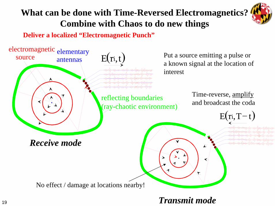
What can be done with Time-Reversed Electromagnetics?Combine with Chaos to do new things

Deliver a localized “Electromagnetic Punch”

Receive mode

( )E r ,tivelectromagnetic

sourceelementaryantennas

reflecting boundaries(ray-chaotic environment)

Put a source emitting a pulse ora known signal at the location ofinterest

Transmit mode

( )E r ,T tiv −

Time-reverse, amplifyand broadcast the coda

No effect / damage at locations nearby!