Chao Zhang Jaswanth Yella Yu Huang

Soft Sensing Transformer:Hundreds of Sensors are Worth a Single Word

Chao ZhangSeagate Technology, MN, USUniversity of Chicago, IL, US

[email protected]

Jaswanth YellaSeagate Technology, MN, US

University of Cincinnati, OH, [email protected]

Yu HuangSeagate Technology, MN, US

Florida Atlantic University, FL, [email protected]

Xiaoye QianSeagate Technology, MN, US

Case Western Reserve University, OH, [email protected]

Sergei PetrovSeagate Technology, MN, USStanford University, CA, [email protected]

Andrey RzhetskyUniversity of Chicago

IL, [email protected]

Sthitie BomSeagate Technology

MN, [email protected]

Abstract—With the rapid development of AI technology inrecent years, there have been many studies with deep learningmodels in soft sensing area. However, the models have becomemore complex, yet, the data sets remain limited: researchersare fitting million-parameter models with hundreds of datasamples, which is insufficient to exercise the effectiveness oftheir models and thus often fail to perform when implementedin industrial applications. To solve this long-lasting problem,we are providing large scale, high dimensional time seriesmanufacturing sensor data from Seagate Technology to thepublic. We demonstrate the challenges and effectiveness ofmodeling industrial big data by a Soft Sensing Transformermodel on these data sets. Transformer is used because, it hasoutperformed state-of-the-art techniques in Natural LanguageProcessing, and since then has also performed well in thedirect application to computer vision without introduction ofimage-specific inductive biases. We observe the similarity ofa sentence structure to the sensor readings and process themulti-variable sensor readings in a time series in a similarmanner of sentences in natural language. The high-dimensionaltime-series data is formatted into the same shape of embeddedsentences and fed into the transformer model. The results showthat transformer model outperforms the benchmark modelsin soft sensing field based on auto-encoder and long short-term memory (LSTM) models. To the best of our knowledge,we are the first team in academia or industry to benchmarkthe performance of original transformer model with large-scale numerical soft sensing data. Additionally, In contrastto the natural language processing or computer vision taskswhere human-level performances are regarded as golden stan-dards, our large scale soft sensing study is an example thattransformer goes beyond human, because the high dimensional

numerical data is not interpretable for human.

1. Introduction

In the last decades, the development of smart sensorshas attracted a lot of attention from government, academiaand industry. The European Union’s 20-20-20 goals (20%increase in energy efficiency, 20% reduction of CO2 emis-sions, and 20% renewable by 2020) rely on smart me-tering as one of their key enablers. Smart meters usuallyinvolve real-time or near real-time sensors, notification andmonitoring. In 2013, Germany proposed the concept ofIndustry 4.0, the main aim of which is to develop smartfactories for producing smart products. The US governmentin September 2020 announced that the US is providingmore than $1 billion towards establishing research and hubsfor Industry 4.0 technologies. Singapore’s current five-yearSU$13.8 billion R&D is injecting more funds into expand-ing fields such as advanced manufacturing. China’s ChinaManufacturing 2025 goal is also to make the manufacturingprocess more intelligent. These initiatives require that wehave better sensing technologies to understand and drive ourprocesses. Sensors have the potential to contain informationabout process variables which can be exploited by data-driven techniques for smarter monitoring and control ofmanufacturing processes. Soft sensing is the general termused for the approaches and the algorithms that are usedto estimate or predict certain physical quantities or productquality in the industrial processes based on the availablesensing modalities, measurements, and knowledge.

As the industrial process have become more complicatedand the size of available data has increased dramatically,there has been growing body of research on deep learning

This paper has been accepted by 2021 IEEE International Conference on Big Data

arX

iv:2

111.

0597

3v1

[cs

.LG

] 1

0 N

ov 2

021

methods with applications in the soft sensing field. A recentsurvey on deep learning methods for soft sensor [1] hasillustrated the significance of the deep learning applicationsand reviewed the most recent studies in this field. Thedeep learning models are mostly based on autoencoder [2],restricted Boltzmann machine [3], convolutional neural net-work [4], and recurrent neural network [5]. The applicationsvaries from traditional factories [6] to wearable IoT devices[7], [8]

There has been a variety of novel deep learning modelssuch as variational autoencoder models which attempts toenhance the representation ability or augment the data [9],[10], semi-supervised ensemble learning model that quan-tifies the contribution of different hidden layers in stackedautoencoder [11], and gated convolutional transformer neu-ral network that combines several state-of-art algorithmstogether to deals with a time-series data set [12]. As thedeep learning models become more and more complex, theircapabilities to handle complex processes and large data setsalso increase. However, in these studies researchers are stillusing very small data sets such as wastewater treatmentplant and Debutanizer column [13], [14] containing lowdimensional data with only hundreds to thousands of datasamples. These small data sets are not sufficient to illustratethe effectiveness of these advanced deep learning modelswith millions of parameters. To solve this issue, we collectedgigabytes of numerical sensor data from Seagate’s wafermanufacturing factories in USA and Ireland. These data setscontain high-dimensional time-series sensor data that is col-lected directly from the Seagate wafer factories with only thenecessary anonymization, and they are big, complex, noisyand impossible to interpret in their raw form by humans..In this article, We evaluate a soft sensing transformer modelagainst the most commonly methods applied to soft sensingproblems including models based on autoencoder and LSTM[15]. The key components of the original transformer modelis maintained and the other parts of the architecture aremodified to fit into our data sets and tasks.

Transformer, since it’s proposal in 2017 [16], togetherwith it’s derivatives such as BERT [17], have been themost active research topic in the natural language processing(NLP) field as well as the top performer in many NLP tasks[18]. Due to its extraordinary representative capability, trans-former model has also shown equally good performance inthe computer vision area [19]. First proposed in 2020, visiontransformer [20] and its variants have achieved the state-of-art performances on many computer vision benchmarks suchas image classification, semantic segmentation and objectdetection [21], [22].

From texts in NLP, which can be regarded as categoricaldata, to images (two dimensional integer values) in computervision, a natural further extension would be soft sensingdata which is time series with continuous floating numbers.While the Bayes error rate [23] in NLP and computer visiontasks are usually defined as human-level performance, oursoft sensing task is impossible for a human to classify basedon the hundreds of sensor values. We show in this paper thatTransformer architecture not only works great for natural

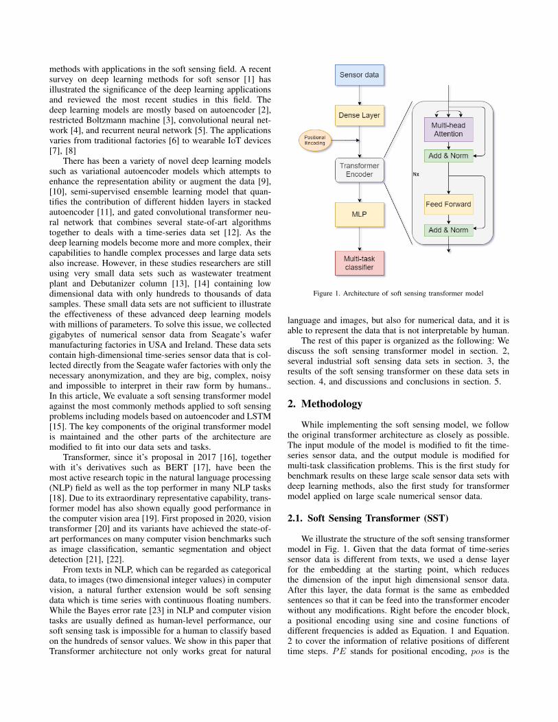
Figure 1. Architecture of soft sensing transformer model

language and images, but also for numerical data, and it isable to represent the data that is not interpretable by human.

The rest of this paper is organized as the following: Wediscuss the soft sensing transformer model in section. 2,several industrial soft sensing data sets in section. 3, theresults of the soft sensing transformer on these data sets insection. 4, and discussions and conclusions in section. 5.

2. Methodology

While implementing the soft sensing model, we followthe original transformer architecture as closely as possible.The input module of the model is modified to fit the time-series sensor data, and the output module is modified formulti-task classification problems. This is the first study forbenchmark results on these large scale sensor data sets withdeep learning methods, also the first study for transformermodel applied on large scale numerical sensor data.

2.1. Soft Sensing Transformer (SST)

We illustrate the structure of the soft sensing transformermodel in Fig. 1. Given that the data format of time-seriessensor data is different from texts, we used a dense layerfor the embedding at the starting point, which reducesthe dimension of the input high dimensional sensor data.After this layer, the data format is the same as embeddedsentences so that it can be feed into the transformer encoderwithout any modifications. Right before the encoder block,a positional encoding using sine and cosine functions ofdifferent frequencies is added as Equation. 1 and Equation.2 to cover the information of relative positions of differenttime steps. PE stands for positional encoding, pos is the

position of a time step, and dmodel is the dimension ofembedded vectors.

PE(pos,2i) = sin(pos/100002i/dmodel) (1)

PE(pos,2i+1) = cos(pos/100002i/dmodel) (2)

Since the SST model requires a fixed size of input data,we added padding to samples with too few time steps sothat each sample has the same time length. The time lengthis chosen as 99 percentiles of the sequence lengths in theraw data to cover most of the data and exclude outliers. Thepadding masks are also applied accordingly. In the encoder,multi-head scaled dot product attention, feed forward andresidual connections are set up in the the same way as inthe original transformer paper [16]. The multi-head attentionis described as in Equation. 3, the query, key and value areprojected to h heads with the weight matrices W q

i ,Wki ,W

vi .

Each head has a dimension of dmodel/h, and a scaled dot-product attention is calculated for each head. Then the headsare concatenated and projected back to the original shape.

MHA(Q,K, V ) = Concat(softmax(QW q

i (KWki )T

√dk

)VWvi )W

o (3)

The Seagate data sets are contain measurement pass/failinformation, and the SST model is built as an classificationmodel. After the encoder blocks, a multi-layer perceptron(MLP) classifier is attached on top after a global averagepooling. Because of the intrinsic complexity of the data,the classifier comprises a few individual binary classifiers.These binary classifiers partly share the input data and maybe correlated with each other, resulting an inter-correlatedmulti-task problem (further discussed in Section. 3). In orderto achieve the best performance in the multi-task learning, aweighting method based on uncertainty [24] is applied, andwe define the combined loss function as Equation. 4:

J =∑i

(1

σ2i

Ji + logσi) (4)

where J is the total loss, Ji is the loss of the ith classifi-cation task, and σi is the uncertainty of the ith classificationloss, which is trainable during the model fitting.

2.2. Optimization

Data imbalance. In the industrial settings, the data arehighly imbalanced. As a classification model, we have only1% to 2% of the data samples as positive. To deal with theimbalance, we experimented on both weighting methods anddata sampling algorithms like SMOTE [25]. We found thatclass weighting gives the best efficiency and performance inour experiments. The weight of the jth task, label t (0 or1) is calculated based on the number of samples:

wtj =

N

2m ∗ ntj(5)

in which N is the total number of sample, m is thenumber of tasks, and ntj is the number of samples for labelt in the jth task.

Combined with the uncertainty based multi-task learningas Equation. 4, the final loss function of SST model isdefined as weighted cross entropy:

J =

m∑j

1∑t=0

[1

σ2jt

ntj∑i

(yijt ∗ logyijt) + log(σjt)] (6)

where yijt and yijt are the true labels and predictedprobabilities for the ith sample in task j for label t. Notethat the cross entropy loss is calculated in a multi-labelclassification manner and the loss for positive and nega-tive cases are computed separately. We take yij1 = 1 forpositive samples, and yij0 = 1 for negative samples. Theweights for the positive and negative cases in a single binaryclassification task is also further tuned by σjt, which is theuncertainty or variance of the loss for label t in task j. Inthis multi-task learning setting, we have 2m ’tasks’ for them binary classifications.

Activation functions. For the transformer encoder part,a ReLU activation function [26] is applied in the feedforward layer, which is consist of two dense layers thatproject the dmodel dimensional vector to dff dimensionand project back to dmodel dimension, respectively. ReLuactivation function is set for the first dense layer in thefeed forward layers. As for the MLP classifier, we appliedsigmoid activation functions for all three layers because wefound that it produced more stable results than ReLu in thiscase.

Regularization. L2 regularizers are applied to all the denselayers in SST model, with a regularization factor of 10−4.Dropout [27] is also applied to residual layers and embed-ding layers. We also applied dropout to each layer in theMLP block except for the final prediction layer. All dropoutratios are kept the same and a grid search in [0.1, 0.3, 0.5]is performed to find the best dropout ratio.

Optimizer. We experimented with two kinds of optimizers:default adam optimizer [28] with fixed learning rate, andscheduled adam optimizer similar as in [16]. The learningrate scheduled optimizer has shown a more stable result, soit’s kept in further experiments.

For the scheduled adam optimizer, the parameters areset as β1 = 0.9, β2 = 0.98, ε = 10−9. The learning rateis varied during the training process based on Equation. 7.d is dmodel in SST model, step is the training step, andwarmup is set as 4000. An extra factor is added to tunethe overall learning rate. A grid search for the factor in[0.1, 0.3, 0.5] is performed to find the optimal factor.

lr = factor ∗ d−0.5 ∗min(step−0.5, step

warmup1.5) (7)

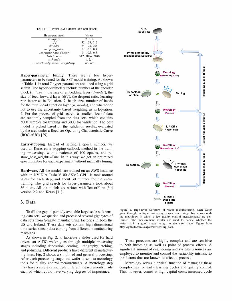
TABLE 1. HYPER-PARAMETER SEARCH SPACE

Hyper-parameter Valuesn layers 2, 3, 4

dff 32, 128, 512dmodel 64, 128, 256

dropout ratio 0.1, 0.3, 0.5learning rate factor 0.1, 0.3, 0.5

batch size 512, 1024, 2048n heads 1, 2, 4

uncertainty based weighting on, off

Hyper-parameter tuning. There are a few hyper-parameters to be tuned for the SST model training. As shownin Table. 1, in total 7 hyper-parameters are tuned using a gridsearch. The hyper-parameters include number of the encoderblock (n layer), the size of embedding layer (dmodel), thesize of feed forward layer (dff ), the dropout ratio, learningrate factor as in Equation. 7, batch size, number of headsfor the multi-head attention layer (n heads), and whether ornot to use the uncertainty based weighting as in Equation.4. For the process of grid search, a smaller size of dataare randomly sampled from the data sets, which contains5000 samples for training and 3000 for validation. The bestmodel is picked based on the validation results, evaluatedby the area under a Receiver Operating Characteristic Curve(ROC-AUC) [29].

Early-stopping. Instead of setting a epoch number, weused an Keras early-stopping callback method in the train-ing processing, with a patience of 100 epochs, and re-store best weights=True. In this way, we got an optimizedepoch number for each experiment without manually tuning.

Hardware. All the models are trained on an AWS instancewith an NVIDIA Tesla V100 SXM2 GPU. It took around20ms for each step, and about 30 minutes for the entiretraining. The grid search for hyper-parameters took about36 hours. All the models are written with TensorFlow [30]version 2.2 and Keras [31].

3. Data

To fill the gap of publicly available large scale soft sens-ing data sets, we queried and processed several gigabytes ofdata sets from Seagate manufacturing factories in both theUS and Ireland. These data sets contain high dimensionaltime-series sensor data coming from different manufacturingmachines.

As shown in Fig. 2, to fabricate a slider used for harddrives, an AlTiC wafer goes through multiple processingstages including deposition, coating, lithography, etching,and polishing. Different products have different manufactur-ing lines, Fig. 2 shows a simplified and general processing.After each processing stage, the wafer is sent to metrologytools for quality control measurements. A metrology stepmay have a single or multiple different measurements madeeach of which could have varying degrees of importance.

Figure 2. High-level workflow of wafer manufacturing. Each wafergoes through multiple processing stages, each stage has correspond-ing metrology, in which a few quality control measurements are per-formed. The measurement results are used to decide whether thewafer is in a good shape to go to the next stage. Figure fromhttps://github.com/Seagate/softsensing data.

These processes are highly complex and are sensitiveto both incoming as well as point of process effects. Asignificant amount of engineering and systems resources areemployed to monitor and control the variability intrinsic tothe factors that are known to affect a process.

Metrology serves a critical function of managing thesecomplexities for early learning cycles and quality control.This, however, comes at high capital costs, increased cycle

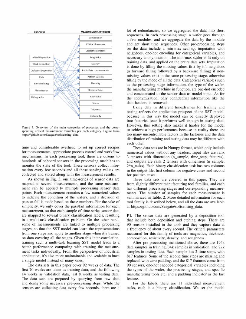
Figure 3. Overview of the main categories of processes and the corre-sponding critical measurement variables per each category. Figure fromhttps://github.com/Seagate/softsensing data.

time and considerable overhead to set up correct recipesfor measurements, appropriate process control and workflowmechanisms. In each processing tool, there are dozens tohundreds of onboard sensors in the processing machines tomonitor the state of the tool. These sensors collect infor-mation every few seconds and all these sensing values arecollected and stored along with the measurement results.

As shown in Fig. 3, one time-series of sensor data aremapped to several measurements, and the same measure-ment can be applied to multiple processing sensor datapoints. Each measurement contains a few numerical valuesto indicate the condition of the wafers, and a decision ofpass or fail is made based on these numbers. For the sake ofsimplicity, we only cover the pass/fail information for eachmeasurement, so that each sample of time-series sensor dataare mapped to several binary classification labels, resultingin a multi-task classification problem. On the other hand,some of measurements are linked to multiple processingstages, so that the SST model can learn the representationsfrom one stage and apply to another stage when it’s trainedon data covering all the stages. Given this inter-correlation,training such a multi-task learning SST model leads to abetter performance comparing with training the measure-ment tasks individually. From the perspective of industrialapplication, it’s also more maintainable and scalable to havea single model instead of many ones.

The data sets in this paper cover 92 weeks of data. Thefirst 70 weeks are taken as training data, and the following14 weeks as validation data, last 8 weeks as testing data.The data sets are prepared by querying from raw dataand doing some necessary pre-processing steps. While thesensors are collecting data every few seconds, there are a

lot of redundancies, so we aggregated the data into shortsequences. In each processing stage, a wafer goes througha few modules, and we aggregate the data by the moduleand get short time sequences. Other pre-processing stepson the data include a min-max scaling, imputation withneighbors, one-hot encoding for categorical variables, andnecessary anonymization. The min-max scaler is fit only ontraining data, and applied on the entire data sets. Imputationis done by filling the missing values first by it’s neighbors(a forward filling followed by a backward filling) if non-missing values exist in the same processing stage, otherwisefilling by the mode of all the data. Categorical variables suchas the processing stage information, the type of the wafer,the manufacturing machine in function, are one-hot encodedand concatenated to the sensor data as model input. As forthe anonymization, only confidential information like thedata headers is removed.

Using data in different timezframes for training andtesting reflects the application prospect of the SST model,because in this way the model can be directly deployedinto factories once it performs well enough in testing data.However, this setting also makes it harder for the modelto achieve a high performance because in reality there aretoo many uncontrollable factors in the factories and the datadistribution of training and testing data may be different witheach other.

These data sets are in Numpy format, which only includenumerical values without any headers. Input files are rank3 tensors with dimension (n sample, time step, features),and outputs are rank 2 tensors with dimension (n sample,2*n tasks). Each binary classification task has two columnsin the output file, first column for negative cases and secondfor positive cases.

Three data sets are covered in this paper. They arefrom slightly different manufacturing tool families, and eachhas different processing stages and corresponding measure-ments. The number of samples for each measurement issummarized in Table. 2. More detailed information for eachtool family is described below, and all the data are availableat https://github.com/Seagate/softsensing data.

P1. The sensor data are generated by a deposition toolthat include both deposition and etching steps. There are90 sensors installed in the tools and they capture data ata frequency of about every second. The critical parametersmeasured for this family of tools are magnetics, thickness,composition, resistivity, density, and roughness.

After pre-processing mentioned above, there are 194kdata samples in training, 34k samples in validation, and 27ksamples in testing data. Each sample has 2 time steps, with817 features. Some of the second time steps are missing andreplaced with zero padding, and the 817 features come from90 sensors, one-hot encoded categorical variables includingthe types of the wafer, the processing stages, and specificmanufacturing tools etc, and a padding indicator as the lastfeature.

For the labels, there are 11 individual measurementtasks, each is a binary classification. We set the model

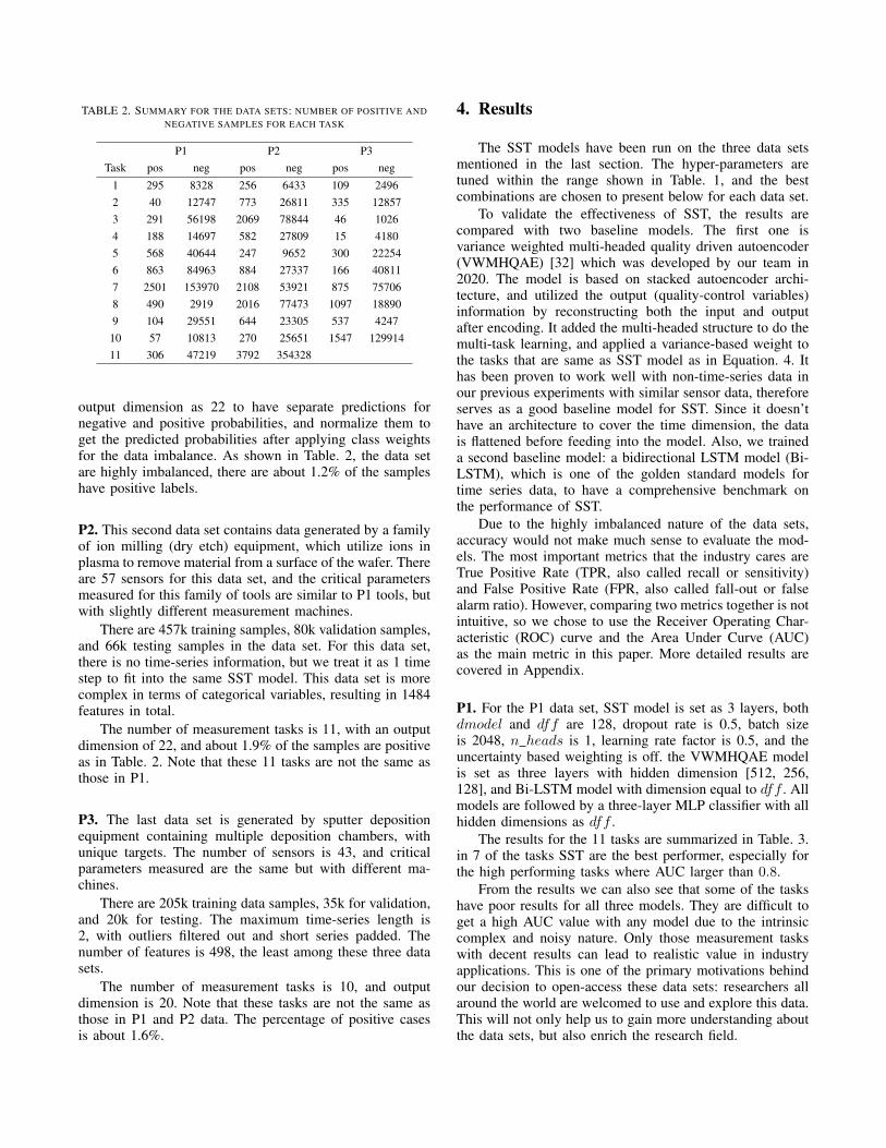
TABLE 2. SUMMARY FOR THE DATA SETS: NUMBER OF POSITIVE ANDNEGATIVE SAMPLES FOR EACH TASK

P1 P2 P3Task pos neg pos neg pos neg

1 295 8328 256 6433 109 24962 40 12747 773 26811 335 128573 291 56198 2069 78844 46 10264 188 14697 582 27809 15 41805 568 40644 247 9652 300 222546 863 84963 884 27337 166 408117 2501 153970 2108 53921 875 757068 490 2919 2016 77473 1097 188909 104 29551 644 23305 537 424710 57 10813 270 25651 1547 12991411 306 47219 3792 354328

output dimension as 22 to have separate predictions fornegative and positive probabilities, and normalize them toget the predicted probabilities after applying class weightsfor the data imbalance. As shown in Table. 2, the data setare highly imbalanced, there are about 1.2% of the sampleshave positive labels.

P2. This second data set contains data generated by a familyof ion milling (dry etch) equipment, which utilize ions inplasma to remove material from a surface of the wafer. Thereare 57 sensors for this data set, and the critical parametersmeasured for this family of tools are similar to P1 tools, butwith slightly different measurement machines.

There are 457k training samples, 80k validation samples,and 66k testing samples in the data set. For this data set,there is no time-series information, but we treat it as 1 timestep to fit into the same SST model. This data set is morecomplex in terms of categorical variables, resulting in 1484features in total.

The number of measurement tasks is 11, with an outputdimension of 22, and about 1.9% of the samples are positiveas in Table. 2. Note that these 11 tasks are not the same asthose in P1.

P3. The last data set is generated by sputter depositionequipment containing multiple deposition chambers, withunique targets. The number of sensors is 43, and criticalparameters measured are the same but with different ma-chines.

There are 205k training data samples, 35k for validation,and 20k for testing. The maximum time-series length is2, with outliers filtered out and short series padded. Thenumber of features is 498, the least among these three datasets.

The number of measurement tasks is 10, and outputdimension is 20. Note that these tasks are not the same asthose in P1 and P2 data. The percentage of positive casesis about 1.6%.

4. Results

The SST models have been run on the three data setsmentioned in the last section. The hyper-parameters aretuned within the range shown in Table. 1, and the bestcombinations are chosen to present below for each data set.

To validate the effectiveness of SST, the results arecompared with two baseline models. The first one isvariance weighted multi-headed quality driven autoencoder(VWMHQAE) [32] which was developed by our team in2020. The model is based on stacked autoencoder archi-tecture, and utilized the output (quality-control variables)information by reconstructing both the input and outputafter encoding. It added the multi-headed structure to do themulti-task learning, and applied a variance-based weight tothe tasks that are same as SST model as in Equation. 4. Ithas been proven to work well with non-time-series data inour previous experiments with similar sensor data, thereforeserves as a good baseline model for SST. Since it doesn’thave an architecture to cover the time dimension, the datais flattened before feeding into the model. Also, we traineda second baseline model: a bidirectional LSTM model (Bi-LSTM), which is one of the golden standard models fortime series data, to have a comprehensive benchmark onthe performance of SST.

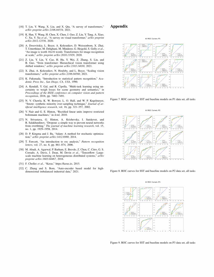
Due to the highly imbalanced nature of the data sets,accuracy would not make much sense to evaluate the mod-els. The most important metrics that the industry cares areTrue Positive Rate (TPR, also called recall or sensitivity)and False Positive Rate (FPR, also called fall-out or falsealarm ratio). However, comparing two metrics together is notintuitive, so we chose to use the Receiver Operating Char-acteristic (ROC) curve and the Area Under Curve (AUC)as the main metric in this paper. More detailed results arecovered in Appendix.

P1. For the P1 data set, SST model is set as 3 layers, bothdmodel and dff are 128, dropout rate is 0.5, batch sizeis 2048, n heads is 1, learning rate factor is 0.5, and theuncertainty based weighting is off. the VWMHQAE modelis set as three layers with hidden dimension [512, 256,128], and Bi-LSTM model with dimension equal to dff . Allmodels are followed by a three-layer MLP classifier with allhidden dimensions as dff .

The results for the 11 tasks are summarized in Table. 3.in 7 of the tasks SST are the best performer, especially forthe high performing tasks where AUC larger than 0.8.

From the results we can also see that some of the taskshave poor results for all three models. They are difficult toget a high AUC value with any model due to the intrinsiccomplex and noisy nature. Only those measurement taskswith decent results can lead to realistic value in industryapplications. This is one of the primary motivations behindour decision to open-access these data sets: researchers allaround the world are welcomed to use and explore this data.This will not only help us to gain more understanding aboutthe data sets, but also enrich the research field.

TABLE 3. RESULT COMPARISON WITH BASELINE MODELS: P1

Task SST VWMHQAE Bi-LSTM

1 0.70± 0.12 0.63± 0.12 0.73 ± 0.13

2 0.60 ± 0.18 0.54± 0.03 0.56± 0.01

3 0.86 ± 0.01 0.77± 0.05 0.86 ± 0.03

4 0.91 ± 0.01 0.89± 0.01 0.88± 0.01

5 0.55 ± 0.03 0.55 ± 0.02 0.51± 0.05

6 0.53± 0.05 0.57 ± 0.03 0.50± 0.03

7 0.64± 0.02 0.65 ± 0.01 0.64± 0.01

8 0.82 ± 0.03 0.78± 0.04 0.78± 0.11

9 0.71± 0.09 0.77 ± 0.01 0.77 ± 0.06

10 0.92 ± 0.03 0.82± 0.03 0.67± 0.23

11 0.89 ± 0.01 0.77± 0.03 0.88± 0.01

Figure 4. ROC curve for SST and baseline models on P1 data set, 4th task

To further illustrate the results, the ROC curve is plot-ted for the task with highest AUC as in Fig. 4. SSThas a higher score than the two baseline models, andthe curve is smoother, meaning a more even distribu-tion of the prediction probabilities and a finer grid inthe prediction space. The source code can be found athttps://github.com/Seagate/SoftSensingTransformer.

P2. SST model is set as 3 layers, both dmodel and dffare 128, dropout rate is 0.3, batch size is 2048, n headsis 1, learning rate factor is 0.5, and the uncertainty basedweighting is on. Baseline models are the same as P1.

The results for the 11 tasks are summarized in Table. 4.SST is the best performer in 4 of the tasks, including thetwo tasks with the best prediction. Same as in P1, some ofthe tasks have poor results for all three models due to theintrinsic complexity and noise in the data set, and we mostlycare about the tasks with best results. In this data set, there isonly one time step, and as expected the VWMHQAE model,which is not designed for time series data, is showing betterresults comparing to P1 data, and it has the best performancein 5 out of the 11 tasks.

The ROC curve for the task with highest AUC as inFig. 5 is very similar to the previous one. SST is slightlysmoother than the baseline models, with a higher AUC.



1 0.89 ± 0.01 0.87± 0.02 0.88± 0.04

2 0.64± 0.01 0.66 ± 0.02 0.59± 0.07

3 0.60± 0.06 0.62 ± 0.01 0.55± 0.01

4 0.85 ± 0.01 0.82± 0.01 0.84± 0.01

5 0.45± 0.07 0.53 ± 0.10 0.52± 0.10

6 0.64± 0.02 0.71± 0.04 0.72 ± 0.02

7 0.78± 0.01 0.81 ± 0.02 0.79± 0.01

8 0.72 ± 0.03 0.70± 0.09 0.69± 0.03

9 0.71± 0.12 0.77 ± 0.08 0.48 ± 0.14

10 0.76 ± 0.02 0.75± 0.01 0.76 ± 0.04

11 0.79± 0.01 0.80± 0.01 0.82 ± 0.01

Figure 5. ROC curve for SST and baseline models on P2 data set, 1st task



1 0.42 ± 0.08 0.23± 0.12 0.32± 0.08

2 0.94 ± 0.02 0.94 ± 0.02 0.93± 0.01

3 0.68 ± 0.08 0.53± 0.10 0.56± 0.05

4 − − −5 0.53± 0.08 0.65 ± 0.05 0.58± 0.05

6 − − −7 0.60± 0.05 0.56± 0.02 0.61 ± 0.07

8 0.72 ± 0.05 0.62± 0.08 0.65± 0.08

9 − − −10 0.81± 0.01 0.81± 0.01 0.82 ± 0.01

P3. SST model is set as 3 layers, both dmodel and dffare 128, dropout rate is 0.3, batch size is 2048, n headsis 1, learning rate factor is 0.3, and the uncertainty basedweighting is on. Baseline models are the same as P1.

The results for 7 out of 10 tasks are summarized inTable. 5, because the others has too few testing data samples.SST is the best performer in 4 of the tasks, including the firsttask with the best prediction. Some of the tasks have poorresults for all three models and even with an AUC lowerthan 0.5, meaning it’s worse than a random guess. Its maincause is the distribution shift and further experiments will

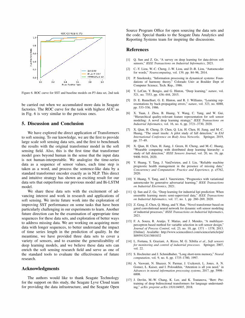
Figure 6. ROC curve for SST and baseline models on P3 data set, 2nd task

be carried out when we accumulated more data in Seagatefactories. The ROC curve for the task with highest AUC asin Fig. 6 is very similar to the previous ones.

5. Discussion and Conclusion

We have explored the direct application of Transformersto soft sensing. To our knowledge, we are the first to providelarge scale soft sensing data sets, and the first to benchmarkthe results with the original transformer model in the softsensing field. Also, this is the first time that transformermodel goes beyond human in the sense that the input datais not human-interpretable. We analogize the time-seriesdata as a sequence of sensor values, each time step istaken as a word, and process the sentence-like data by astandard transformer encoder exactly as in NLP. This directand intuitive strategy has shown an exciting result for ourdata sets that outperforms our previous model and Bi-LSTMmodel.

We share these data sets with the excitement of ad-vancing interest and work in research and applications ofsoft sensing. We invite future work into the exploration ofimproving SST performance on some tasks that have beenparticularly challenging in our experiments to learn. Anotherfuture direction can be the examination of appropriate timesequences for these data sets, and exploration of better waysto address missing data. We are working on acquiring moredata with longer sequences, to better understand the impactof time series length in the prediction of quality. In themeantime, we have provided three data sets to cover avariety of sensors, and to examine the generalizability ofdeep learning models, and we believe these data sets canenrich the soft sensing research field and serve as one ofthe standard tools to evaluate the effectiveness of futureresearch.

Acknowledgments

The authors would like to thank Seagate Technologyfor the support on this study, the Seagate Lyve Cloud teamfor providing the data infrastructure, and the Seagate Open

Source Program Office for open sourcing the data sets andthe code. Special thanks to the Seagate Data Analytics andReporting Systems team for inspiring the discussions.

References

[1] Q. Sun and Z. Ge, “A survey on deep learning for data-driven softsensors,” IEEE Transactions on Industrial Informatics, 2021.

[2] C.-Y. Liou, W.-C. Cheng, J.-W. Liou, and D.-R. Liou, “Autoencoderfor words,” Neurocomputing, vol. 139, pp. 84–96, 2014.

[3] P. Smolensky, “Information processing in dynamical systems: Foun-dations of harmony theory,” Colorado Univ at Boulder Dept ofComputer Science, Tech. Rep., 1986.

[4] Y. LeCun, Y. Bengio, and G. Hinton, “Deep learning,” nature, vol.521, no. 7553, pp. 436–444, 2015.

[5] D. E. Rumelhart, G. E. Hinton, and R. J. Williams, “Learning rep-resentations by back-propagating errors,” nature, vol. 323, no. 6088,pp. 533–536, 1986.

[6] X. Yuan, J. Zhou, B. Huang, Y. Wang, C. Yang, and W. Gui,“Hierarchical quality-relevant feature representation for soft sensormodeling: A novel deep learning strategy,” IEEE Transactions onIndustrial Informatics, vol. 16, no. 6, pp. 3721–3730, 2020.

[7] X. Qian, H. Cheng, D. Chen, Q. Liu, H. Chen, H. Jiang, and M.-C.Huang, “The smart insole: A pilot study of fall detection,” in EAIInternational Conference on Body Area Networks. Springer, 2019,pp. 37–49.

[8] X. Qian, H. Chen, H. Jiang, J. Green, H. Cheng, and M.-C. Huang,“Wearable computing with distributed deep learning hierarchy: astudy of fall detection,” IEEE Sensors Journal, vol. 20, no. 16, pp.9408–9416, 2020.

[9] Y. Huang, Y. Tang, J. VanZwieten, and J. Liu, “Reliable machineprognostic health management in the presence of missing data,”Concurrency and Computation: Practice and Experience, p. e5762,2020.

[10] Y. Huang, Y. Tang, and J. Vanzwieten, “Prognostics with variationalautoencoder by generative adversarial learning,” IEEE Transactionson Industrial Electronics, 2021.

[11] Q. Sun and Z. Ge, “Deep learning for industrial kpi prediction: Whenensemble learning meets semi-supervised data,” IEEE Transactionson Industrial Informatics, vol. 17, no. 1, pp. 260–269, 2020.

[12] Z. Geng, Z. Chen, Q. Meng, and Y. Han, “Novel transformer based ongated convolutional neural network for dynamic soft sensor modelingof industrial processes,” IEEE Transactions on Industrial Informatics,2021.

[13] F. A. Souza, R. Araujo, T. Matias, and J. Mendes, “A multilayer-perceptron based method for variable selection in soft sensor design,”Journal of Process Control, vol. 23, no. 10, pp. 1371 – 1378, 2013.[Online]. Available: http://www.sciencedirect.com/science/article/pii/S0959152413001832

[14] L. Fortuna, S. Graziani, A. Rizzo, M. G. Xibilia et al., Soft sensorsfor monitoring and control of industrial processes. Springer, 2007,vol. 22.

[15] S. Hochreiter and J. Schmidhuber, “Long short-term memory,” Neuralcomputation, vol. 9, no. 8, pp. 1735–1780, 1997.

[16] A. Vaswani, N. Shazeer, N. Parmar, J. Uszkoreit, L. Jones, A. N.Gomez, Ł. Kaiser, and I. Polosukhin, “Attention is all you need,” inAdvances in neural information processing systems, 2017, pp. 5998–6008.

[17] J. Devlin, M.-W. Chang, K. Lee, and K. Toutanova, “Bert: Pre-training of deep bidirectional transformers for language understand-ing,” arXiv preprint arXiv:1810.04805, 2018.

http://www.sciencedirect.com/science/article/pii/S0959152413001832

http://www.sciencedirect.com/science/article/pii/S0959152413001832

[18] T. Lin, Y. Wang, X. Liu, and X. Qiu, “A survey of transformers,”arXiv preprint arXiv:2106.04554, 2021.

[19] K. Han, Y. Wang, H. Chen, X. Chen, J. Guo, Z. Liu, Y. Tang, A. Xiao,C. Xu, Y. Xu et al., “A survey on visual transformer,” arXiv preprintarXiv:2012.12556, 2020.

[20] A. Dosovitskiy, L. Beyer, A. Kolesnikov, D. Weissenborn, X. Zhai,T. Unterthiner, M. Dehghani, M. Minderer, G. Heigold, S. Gelly et al.,“An image is worth 16x16 words: Transformers for image recognitionat scale,” arXiv preprint arXiv:2010.11929, 2020.

[21] Z. Liu, Y. Lin, Y. Cao, H. Hu, Y. Wei, Z. Zhang, S. Lin, andB. Guo, “Swin transformer: Hierarchical vision transformer usingshifted windows,” arXiv preprint arXiv:2103.14030, 2021.

[22] X. Zhai, A. Kolesnikov, N. Houlsby, and L. Beyer, “Scaling visiontransformers,” arXiv preprint arXiv:2106.04560, 2021.

[23] K. Fukunada, “Introduction to statistical pattern recognition,” Aca-demic Press Inc., San Diego, CA, USA, 1990.

[24] A. Kendall, Y. Gal, and R. Cipolla, “Multi-task learning using un-certainty to weigh losses for scene geometry and semantics,” inProceedings of the IEEE conference on computer vision and patternrecognition, 2018, pp. 7482–7491.

[25] N. V. Chawla, K. W. Bowyer, L. O. Hall, and W. P. Kegelmeyer,“Smote: synthetic minority over-sampling technique,” Journal of ar-tificial intelligence research, vol. 16, pp. 321–357, 2002.

[26] V. Nair and G. E. Hinton, “Rectified linear units improve restrictedboltzmann machines,” in Icml, 2010.

[27] N. Srivastava, G. Hinton, A. Krizhevsky, I. Sutskever, andR. Salakhutdinov, “Dropout: a simple way to prevent neural networksfrom overfitting,” The journal of machine learning research, vol. 15,no. 1, pp. 1929–1958, 2014.

[28] D. P. Kingma and J. Ba, “Adam: A method for stochastic optimiza-tion,” arXiv preprint arXiv:1412.6980, 2014.

[29] T. Fawcett, “An introduction to roc analysis,” Pattern recognitionletters, vol. 27, no. 8, pp. 861–874, 2006.

[30] M. Abadi, A. Agarwal, P. Barham, E. Brevdo, Z. Chen, C. Citro, G. S.Corrado, A. Davis, J. Dean, M. Devin et al., “Tensorflow: Large-scale machine learning on heterogeneous distributed systems,” arXivpreprint arXiv:1603.04467, 2016.

[31] F. Chollet et al., “Keras,” https://keras.io, 2015.

[32] C. Zhang and S. Bom, “Auto-encoder based model for high-dimensional imbalanced industrial data,” 2021.

Appendix

Figure 7. ROC curves for SST and baseline models on P1 data set, all tasks



https://keras.io

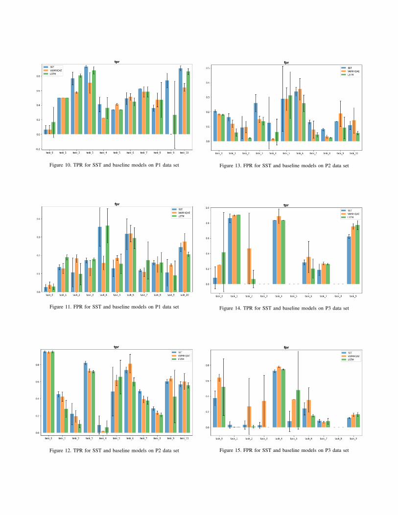
Figure 10. TPR for SST and baseline models on P1 data set

Figure 11. FPR for SST and baseline models on P1 data set





Documents

Chao Zhang Jaswanth Yella Yu Huang