Embed Size (px)
DESCRIPTION
Channel Routing
Citation preview
1
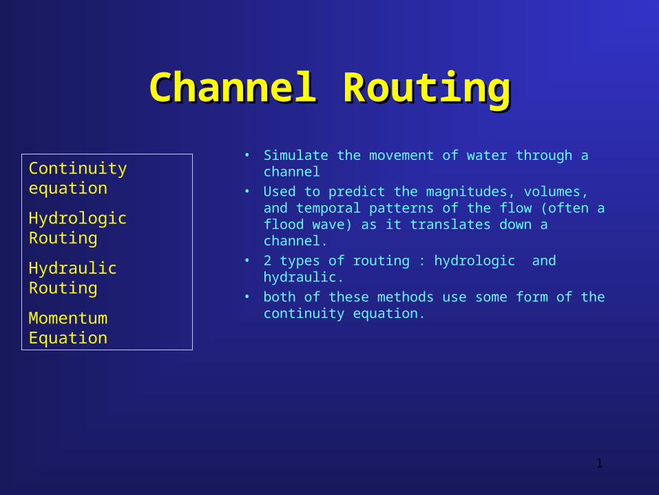
Channel RoutingChannel Routing
• Simulate the movement of water through a channel
• Used to predict the magnitudes, volumes, and temporal patterns of the flow (often a flood wave) as it translates down a channel.
• 2 types of routing : hydrologic and hydraulic.
• both of these methods use some form of the continuity equation.
Continuity equation
Hydrologic Routing
Hydraulic Routing
Momentum Equation
2
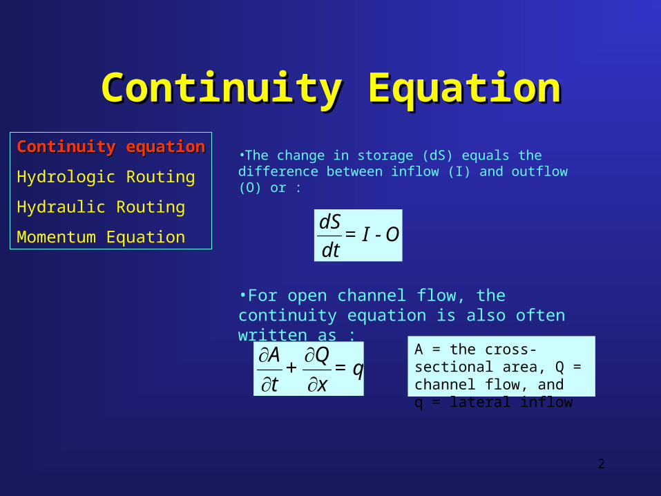
Continuity EquationContinuity Equation
•The change in storage (dS) equals the difference between inflow (I) and outflow (O) or :
O - I = dt
dS
•For open channel flow, the continuity equation is also often written as :
q = x
Q +
t
A
A = the cross-sectional area,
Q = channel flow, and q = lateral inflow
Continuity equationContinuity equation
Hydrologic Routing
Hydraulic Routing
Momentum Equation
3
Hydrologic RoutingHydrologic Routing
• Methods combine the continuity equation with some relationship between storage, outflow, and possibly inflow.
• These relationships are usually assumed, empirical, or analytical in nature.
• An of example of such a relationship might be a stage-discharge relationship.
Continuity equation
Hydrologic RoutingHydrologic Routing
Hydraulic Routing
Momentum Equation
4
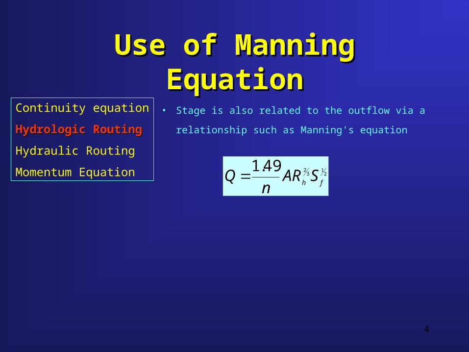
Use of Manning EquationUse of Manning Equation
• Stage is also related to the outflow via a relationship
such as Manning's equation
21
3249.1
fhSAR
nQ
Continuity equation
Hydrologic RoutingHydrologic Routing
Hydraulic Routing
Momentum Equation
5
Hydraulic RoutingHydraulic Routing
• Hydraulic routing methods combine the continuity equation with some more physical relationship describing the actual physics of the movement of the water.
• The momentum equation is the common relationship employed.
• In hydraulic routing analysis, it is intended that the dynamics of the water or flood wave movement be more accurately described
Continuity equation
Hydrologic Routing
Hydraulic RoutingHydraulic Routing
Momentum Equation
6
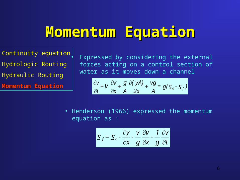
Momentum EquationMomentum Equation
• Expressed by considering the external forces acting on a control section of water as it moves down a channel
)S - Sg( = A
vg +
2x
A)y(
A
g +
x
v V +
t
vfo
• Henderson (1966) expressed the momentum equation as :
t
v
g
1 -
x
v
g
v -
x
y - S = S of
Continuity equation
Hydrologic Routing
Hydraulic Routing
Momentum EquationMomentum Equation
7
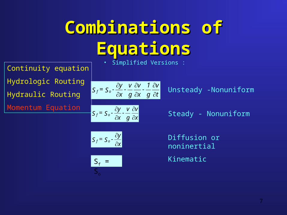
Combinations of EquationsCombinations of Equations• Simplified Versions :
t
v
g
1 -
x
v
g
v -
x
y - S = S of
x
v
g
v -
x
y - S = S of
x
y - S = S of
Sf = So
Unsteady -Nonuniform
Steady - Nonuniform
Diffusion or noninertial
Kinematic
Continuity equation
Hydrologic Routing
Hydraulic Routing
Momentum Equation
8
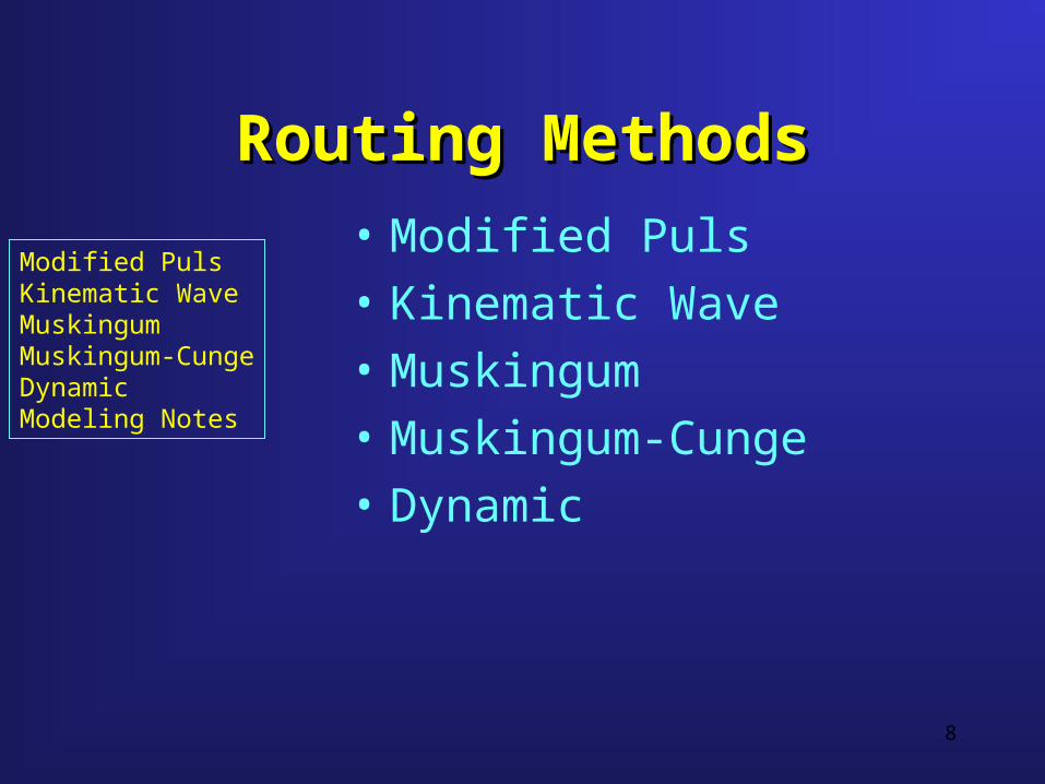
Routing MethodsRouting Methods
• Modified Puls
• Kinematic Wave
• Muskingum
• Muskingum-Cunge
• Dynamic
Modified PulsKinematic WaveMuskingumMuskingum-CungeDynamicModeling Notes
9
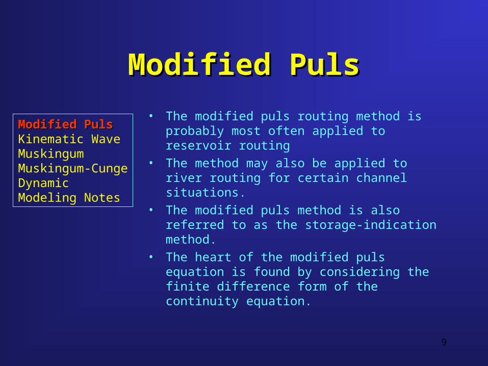
Modified PulsModified Puls
• The modified puls routing method is probably most often applied to reservoir routing
• The method may also be applied to river routing for certain channel situations.
• The modified puls method is also referred to as the storage-indication method.
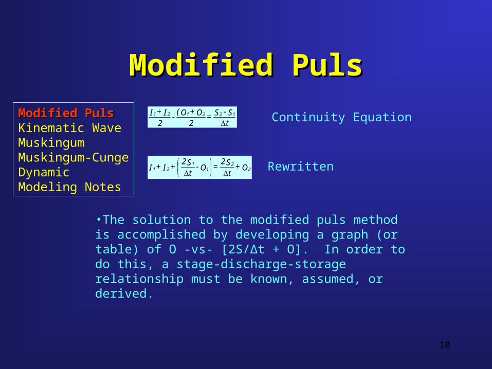
• The heart of the modified puls equation is found by considering the finite difference form of the continuity equation.
Modified PulsModified PulsKinematic WaveMuskingumMuskingum-CungeDynamicModeling Notes
10
Modified PulsModified Puls
tS - S =
2O + O(
- 2
I + I 122121
Continuity Equation
O + t
S2 = O -
tS2
+ I + I 22
11
21
Rewritten
•The solution to the modified puls method is accomplished by developing a graph (or table) of O -vs- [2S/Δt + O]. In order to do this, a stage-discharge-storage relationship must be known, assumed, or derived.
Modified PulsModified PulsKinematic WaveMuskingumMuskingum-CungeDynamicModeling Notes

11
Modified PulsModified Puls
Modified PulsModified PulsKinematic WaveMuskingumMuskingum-CungeDynamicModeling Notes
12
Modified Puls ExampleModified Puls Example
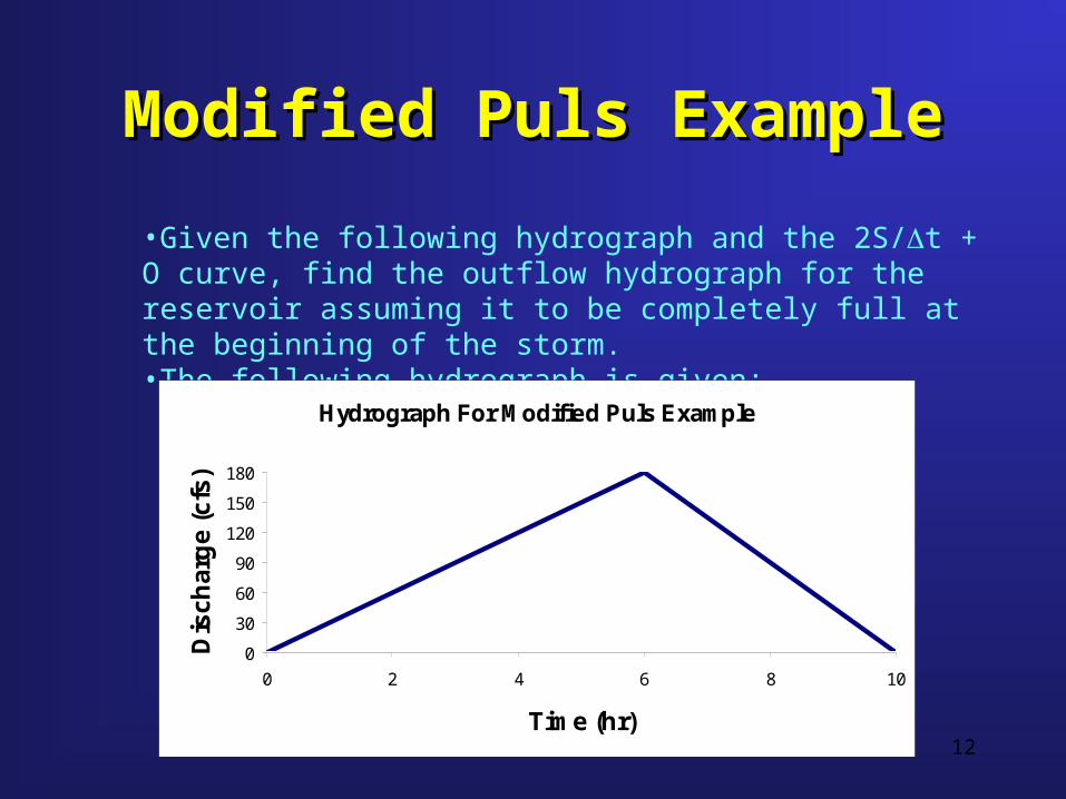
•Given the following hydrograph and the 2S/t + O curve, find the outflow hydrograph for the reservoir assuming it to be completely full at the beginning of the storm.•The following hydrograph is given:
Hydrograph For Modified Puls Example
0
30
60
90
120
150
180
0 2 4 6 8 10
Time (hr)
Dis
ch
arg
e (
cfs
)
13
Modified Puls ExampleModified Puls Example
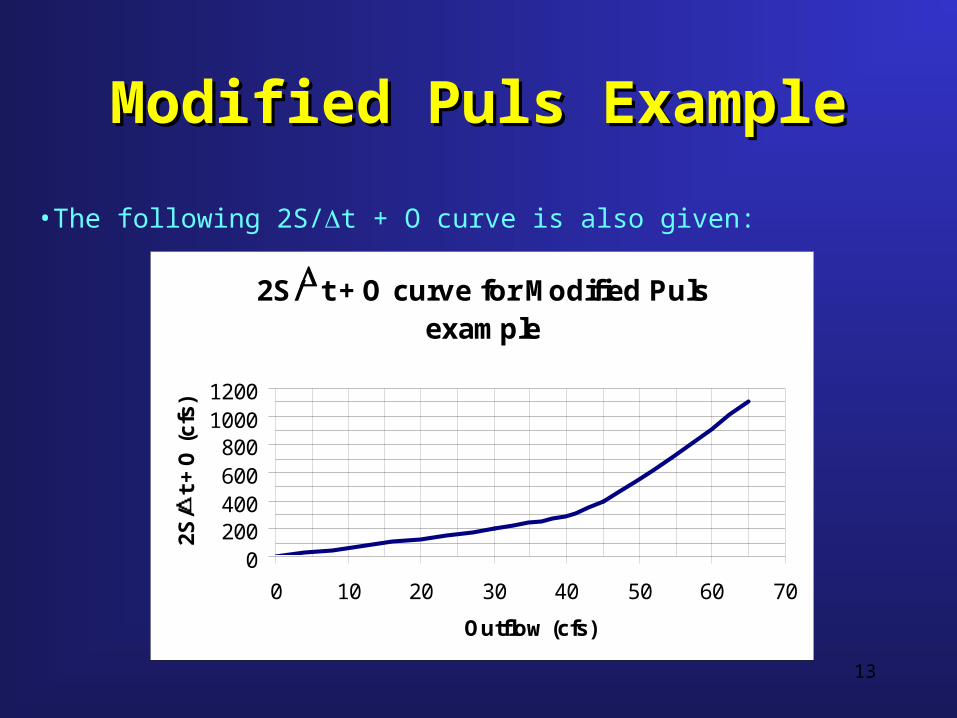
2S/ t + O curve for Modified Puls example
0200400600800
10001200
0 10 20 30 40 50 60 70
Outflow (cfs)
2S
/t
+ O
(c
fs)
•The following 2S/t + O curve is also given:
14
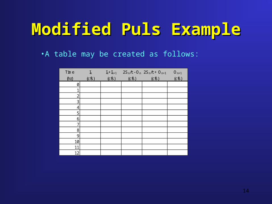
Modified Puls ExampleModified Puls Example•A table may be created as follows:
Time In In+In+1 2Sn/t - On 2Sn/t + On+1 On+1
(hr) (cfs) (cfs) (cfs) (cfs) (cfs)0123456789
101112
15
Modified Puls ExampleModified Puls Example
Hydrograph For Modified Puls Example
0
30
60
90
120
150
180
0 2 4 6 8 10
Time (hr)
Dis
char
ge (c
fs)
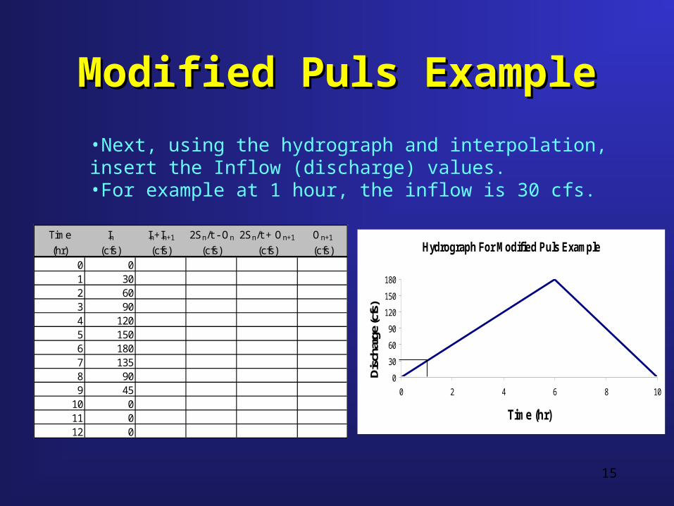
•Next, using the hydrograph and interpolation, insert the Inflow (discharge) values. •For example at 1 hour, the inflow is 30 cfs.
Time In In+In+1 2Sn/t - On 2Sn/t + On+1 On+1
(hr) (cfs) (cfs) (cfs) (cfs) (cfs)0 01 302 603 904 1205 1506 1807 1358 909 45
10 011 012 0
16
Modified Puls ExampleModified Puls Example
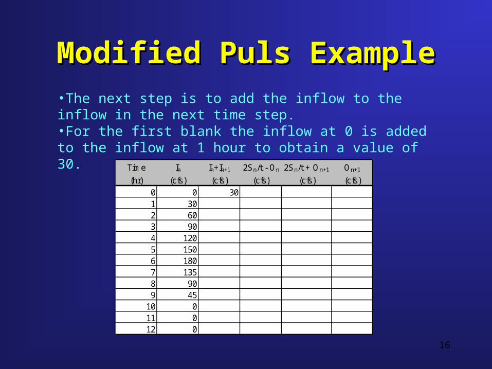
Time In In+In+1 2Sn/t - On 2Sn/t + On+1 On+1
(hr) (cfs) (cfs) (cfs) (cfs) (cfs)0 0 301 302 603 904 1205 1506 1807 1358 909 45
10 011 012 0
•The next step is to add the inflow to the inflow in the next time step.•For the first blank the inflow at 0 is added to the inflow at 1 hour to obtain a value of 30.
17
Modified Puls ExampleModified Puls Example
Time In In+In+1 2Sn/t - On 2Sn/t + On+1 On+1
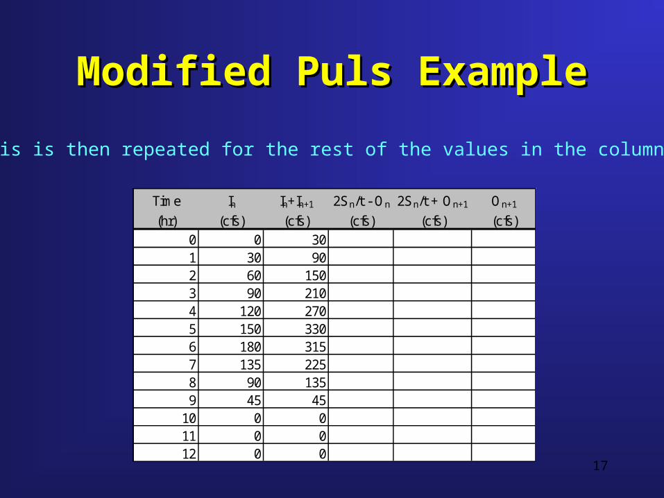
(hr) (cfs) (cfs) (cfs) (cfs) (cfs)0 0 301 30 902 60 1503 90 2104 120 2705 150 3306 180 3157 135 2258 90 1359 45 45
10 0 011 0 012 0 0
•This is then repeated for the rest of the values in the column.
18
Modified Puls ExampleModified Puls Example
Time In In+In+1 2Sn/t - On 2Sn/t + On+1 On+1
(hr) (cfs) (cfs) (cfs) (cfs) (cfs)0 0 30 0 01 30 90 302 60 1503 90 2104 120 2705 150 3306 180 3157 135 2258 90 1359 45 45
10 0 011 0 012 0 0
O + t
S2 = O -
tS2
+ I + I 22
11
21
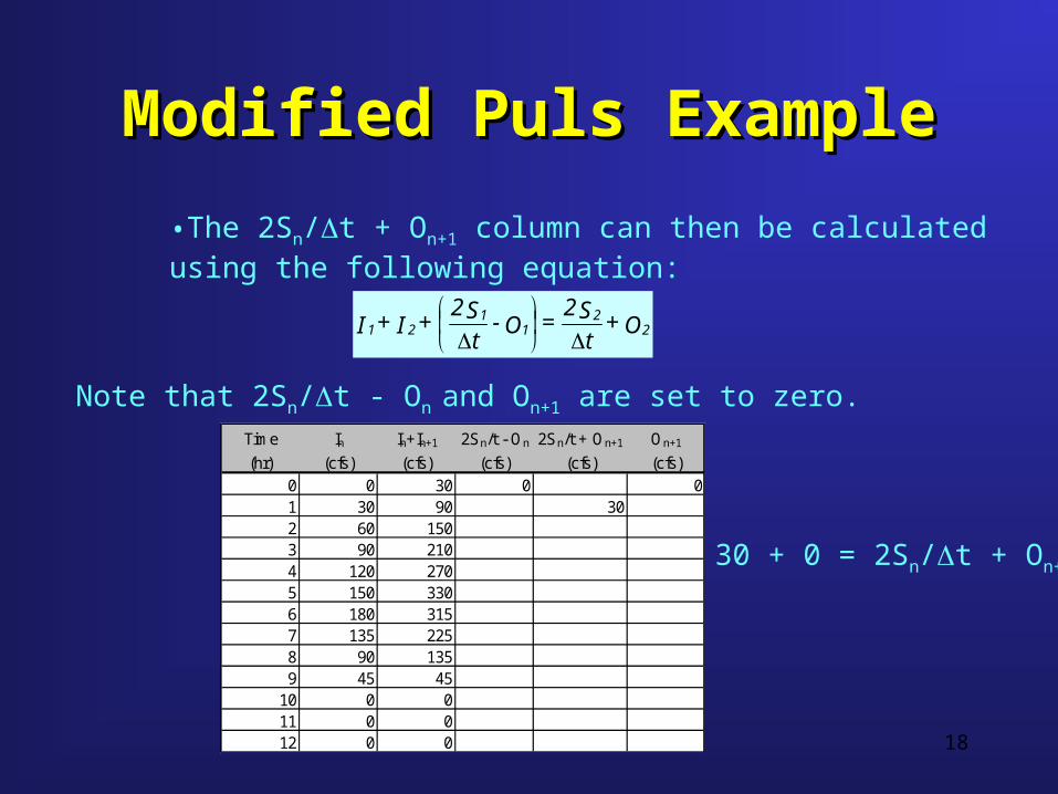
•The 2Sn/t + On+1 column can then be calculated using the following equation:
Note that 2Sn/t - On and On+1 are set to zero.
30 + 0 = 2Sn/t + On+1
19
Modified Puls ExampleModified Puls Example
2S/ t + O curve for Modified Puls example
0200400600800
10001200
0 10 20 30 40 50 60 70
Outflow (cfs)
2S/
t + O
(cfs
)
Time In In+In+1 2Sn/t - On 2Sn/t + On+1 On+1
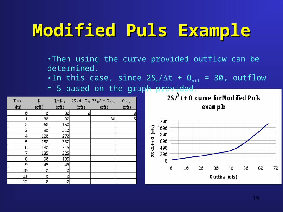
(hr) (cfs) (cfs) (cfs) (cfs) (cfs)0 0 30 0 01 30 90 30 52 60 1503 90 2104 120 2705 150 3306 180 3157 135 2258 90 1359 45 45
10 0 011 0 012 0 0
•Then using the curve provided outflow can be determined.•In this case, since 2Sn/t + On+1 = 30, outflow = 5 based on the graph provided.
20
Modified Puls ExampleModified Puls Example
Time In In+In+1 2Sn/t - On 2Sn/t + On+1 On+1
(hr) (cfs) (cfs) (cfs) (cfs) (cfs)0 0 30 0 01 30 90 20 30 52 60 1503 90 2104 120 2705 150 3306 180 3157 135 2258 90 1359 45 45
10 0 011 0 012 0 0
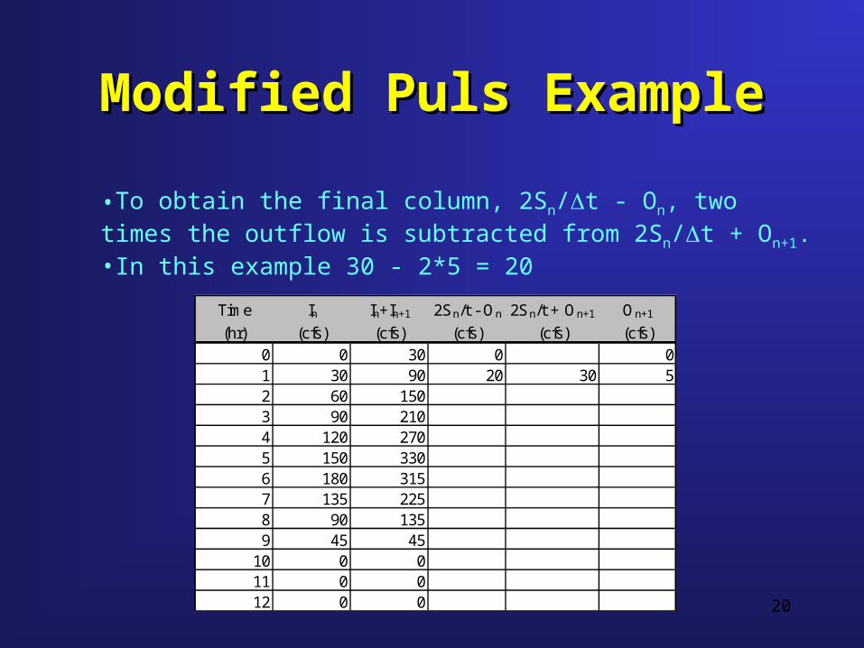
•To obtain the final column, 2Sn/t - On, two times the outflow is subtracted from 2Sn/t + On+1.•In this example 30 - 2*5 = 20
21
Modified Puls ExampleModified Puls Example
Time In In+In+1 2Sn/t - On 2Sn/t + On+1 On+1
(hr) (cfs) (cfs) (cfs) (cfs) (cfs)0 0 30 0 01 30 90 20 30 52 60 150 74 110 183 90 2104 120 2705 150 3306 180 3157 135 2258 90 1359 45 45
10 0 011 0 012 0 0
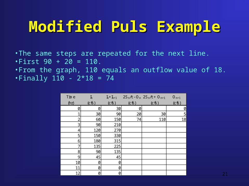
•The same steps are repeated for the next line.•First 90 + 20 = 110.•From the graph, 110 equals an outflow value of 18.•Finally 110 - 2*18 = 74
22
Modified Puls ExampleModified Puls Example
Time In In+In+1 2Sn/t - On 2Sn/t + On+1 On+1
(hr) (cfs) (cfs) (cfs) (cfs) (cfs)0 0 30 0 01 30 90 20 30 52 60 150 74 110 183 90 210 160 224 324 120 270 284 370 435 150 330 450 554 526 180 315 664 780 587 135 225 853 979 638 90 135 948 1078 659 45 45 953 1085 65
10 0 0 870 998 6411 0 0 746 870 6212 0 0 630 746 58
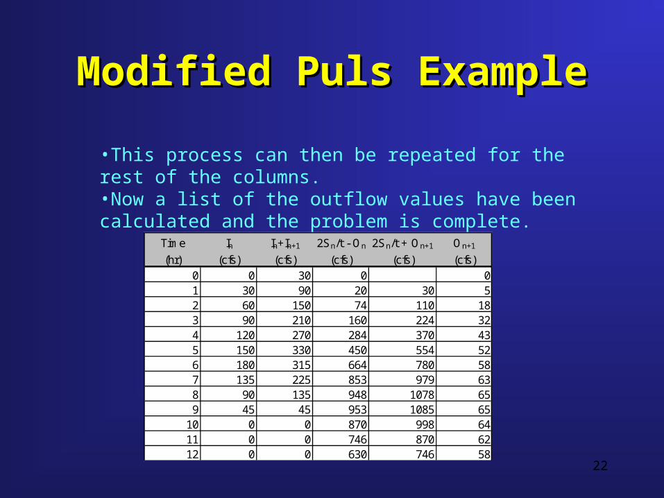
•This process can then be repeated for the rest of the columns.•Now a list of the outflow values have been calculated and the problem is complete.
23
KinematicKinematic WaveWave
• Kinematic wave channel routing is probably the most basic form of hydraulic routing.
• This method combines the continuity equation with a very simplified form of the St. Venant equations.
• Kinematic wave routing assumes that the friction slope is equal to the bed slope.
• Additionally, the kinematic wave form of the momentum equation assumes a simple stage-discharge relationship.
Modified PulsKinematic WaveKinematic WaveMuskingumMuskingum-CungeDynamicModeling Notes
24
KinematicKinematic WaveWave BasicBasic EquationsEquations
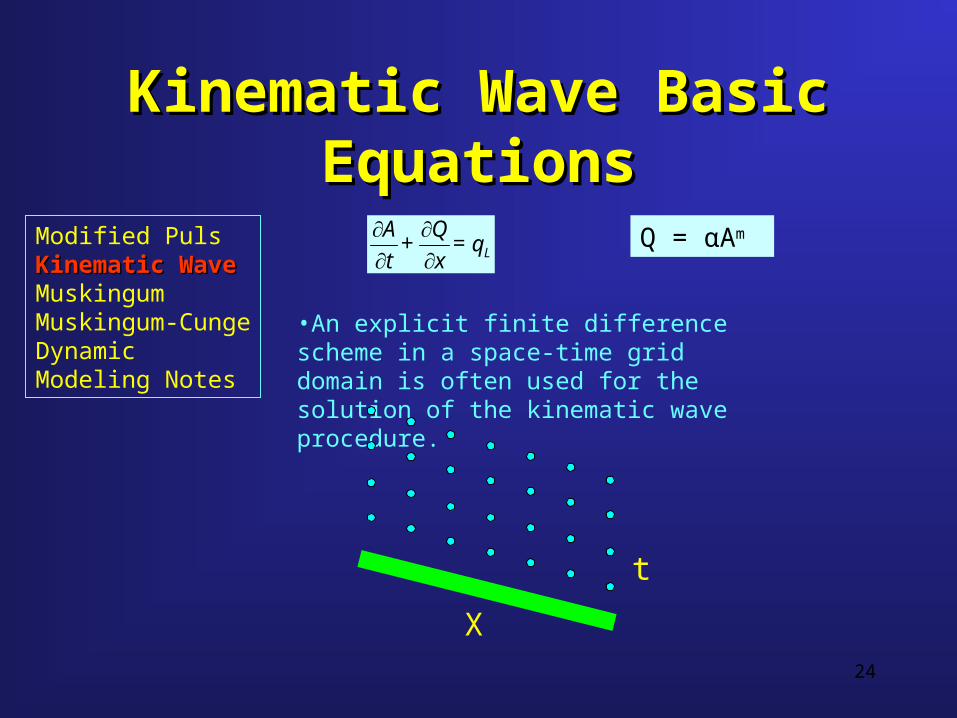
q = x
Q +
t
AL
Q = αAm
•An explicit finite difference scheme in a space-time grid domain is often used for the solution of the kinematic wave procedure.
X
t
Modified PulsKinematic WaveKinematic WaveMuskingumMuskingum-CungeDynamicModeling Notes
25
WorkingWorking EquationEquation
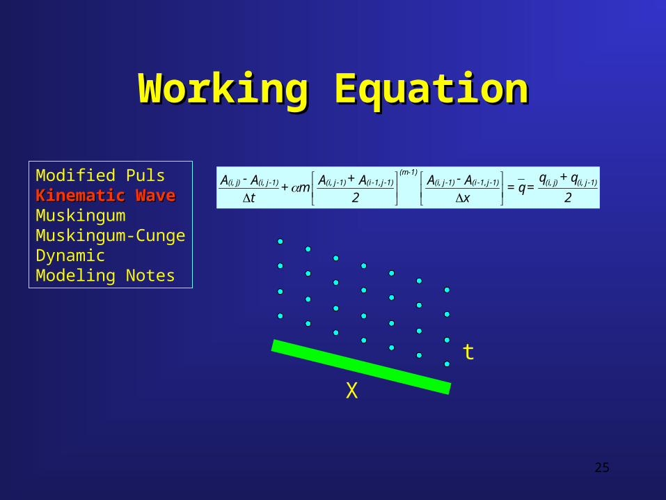
2
q + q = q =
xA - A
2A + A m +
tA - A 1)-j(i,j)(i,1)-j1,-(i1)-j(i,1)-j1,-(i1)-j(i,
1)-(m1)-j(i,j)(i,
X
t
Modified PulsKinematic WaveKinematic WaveMuskingumMuskingum-CungeDynamicModeling Notes
26
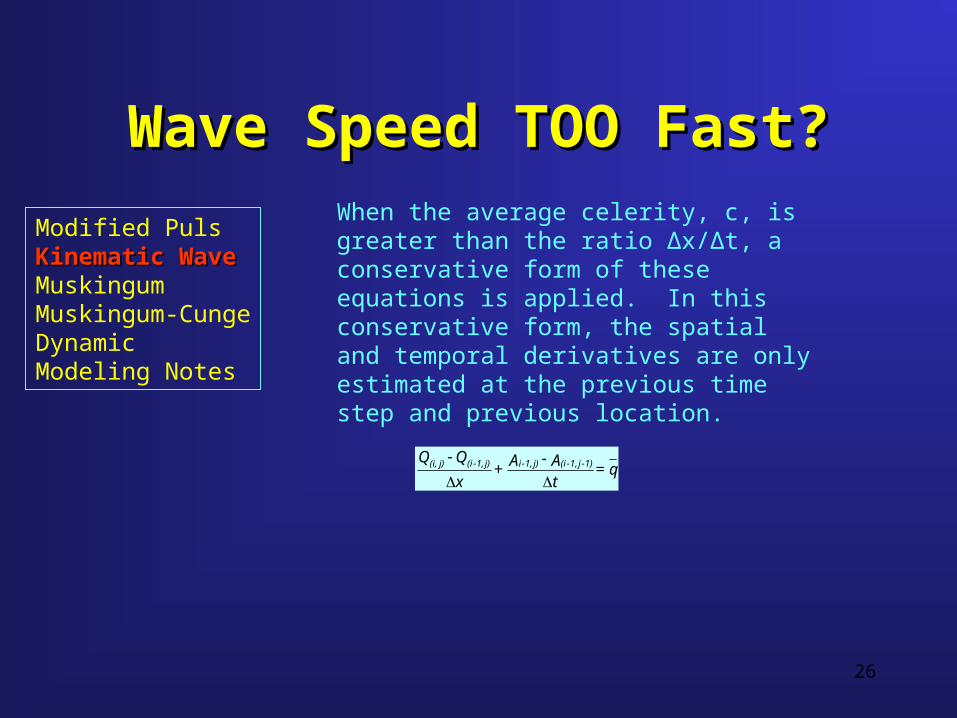
WaveWave SpeedSpeed TOOTOO Fast?Fast?When the average celerity, c, is greater than the ratio Δx/Δt, a conservative form of these equations is applied. In this conservative form, the spatial and temporal derivatives are only estimated at the previous time step and previous location.
q = tA - A +
x
Q - Q 1)-j1,-(ij)1,-ij)1,-(ij)(i,
Modified PulsKinematic WaveKinematic WaveMuskingumMuskingum-CungeDynamicModeling Notes
27
KinematicKinematic WaveWave AssumptionsAssumptions
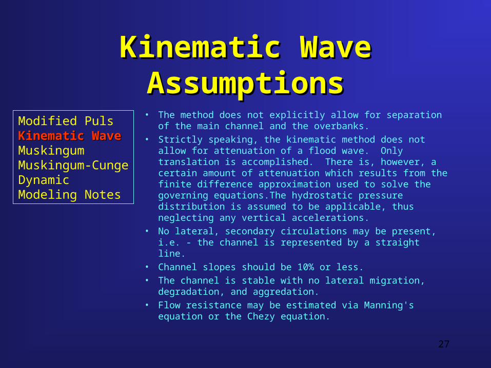
• The method does not explicitly allow for separation of the main channel and the overbanks.
• Strictly speaking, the kinematic method does not allow for attenuation of a flood wave. Only translation is accomplished. There is, however, a certain amount of attenuation which results from the finite difference approximation used to solve the governing equations.The hydrostatic pressure distribution is assumed to be applicable, thus neglecting any vertical accelerations.
• No lateral, secondary circulations may be present, i.e. - the channel is represented by a straight line.
• Channel slopes should be 10% or less.
• The channel is stable with no lateral migration, degradation, and aggredation.
• Flow resistance may be estimated via Manning's equation or the Chezy equation.
Modified PulsKinematic WaveKinematic WaveMuskingumMuskingum-CungeDynamicModeling Notes
28
MuskingumMuskingum MethodMethod
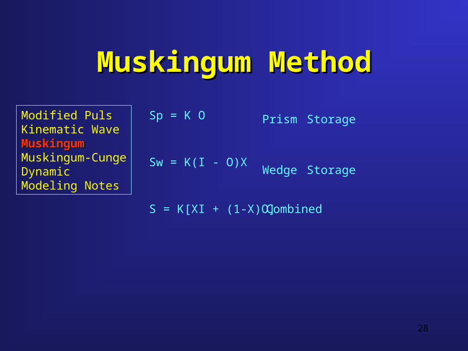
Sp = K O
Sw = K(I - O)X
Prism Storage
Wedge Storage
CombinedS = K[XI + (1-X)O]
Modified PulsKinematic WaveMuskingumMuskingumMuskingum-CungeDynamicModeling Notes
29
Muskingum,Muskingum, cont...cont...
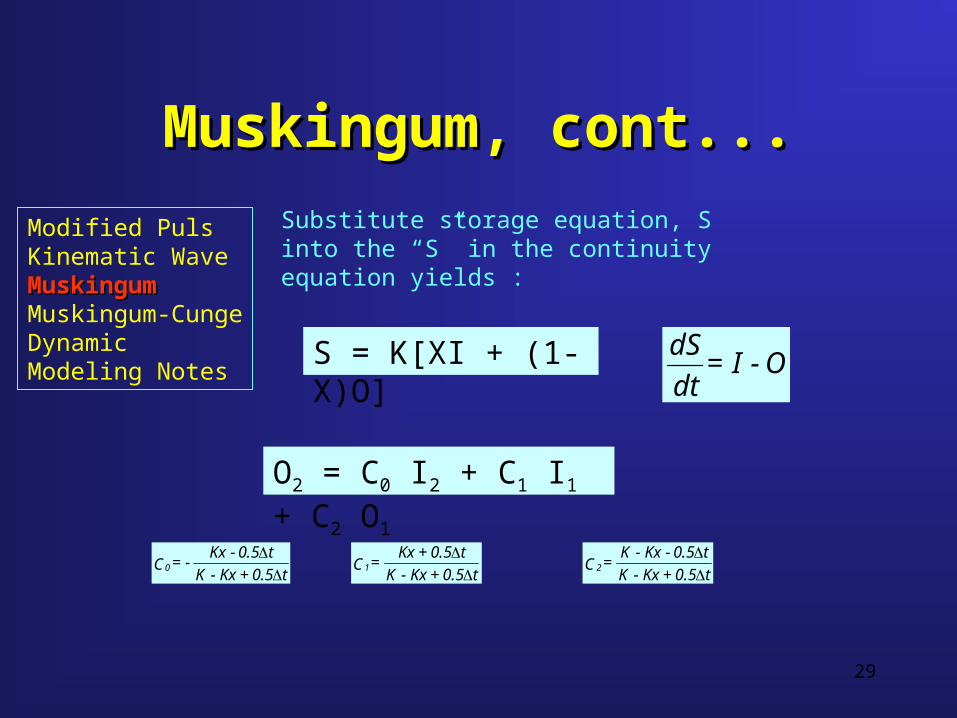
O2 = C0 I2 + C1 I1 + C2 O1
Substitute storage equation, S into the “S” in the continuity equation yields :
S = K[XI + (1-X)O] O - I = dt
dS
t0.5 + Kx - K
t0.5 - Kx - = C0
t0.5 + Kx - K
t0.5 + Kx = C1
t0.5 + Kx - K
t0.5 - Kx - K = C2
Modified PulsKinematic WaveMuskingumMuskingumMuskingum-CungeDynamicModeling Notes
30
Muskingum Notes :Muskingum Notes :
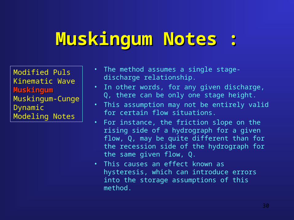
• The method assumes a single stage-discharge relationship.
• In other words, for any given discharge, Q, there can be only one stage height.
• This assumption may not be entirely valid for certain flow situations.
• For instance, the friction slope on the rising side of a hydrograph for a given flow, Q, may be quite different than for the recession side of the hydrograph for the same given flow, Q.
• This causes an effect known as hysteresis, which can introduce errors into the storage assumptions of this method.
Modified PulsKinematic WaveMuskingumMuskingumMuskingum-CungeDynamicModeling Notes
31
Estimating KEstimating K
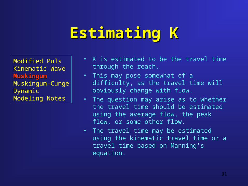
• K is estimated to be the travel time through the reach.
• This may pose somewhat of a difficulty, as the travel time will obviously change with flow.
• The question may arise as to whether the travel time should be estimated using the average flow, the peak flow, or some other flow.
• The travel time may be estimated using the kinematic travel time or a travel time based on Manning's equation.
Modified PulsKinematic WaveMuskingumMuskingumMuskingum-CungeDynamicModeling Notes
32
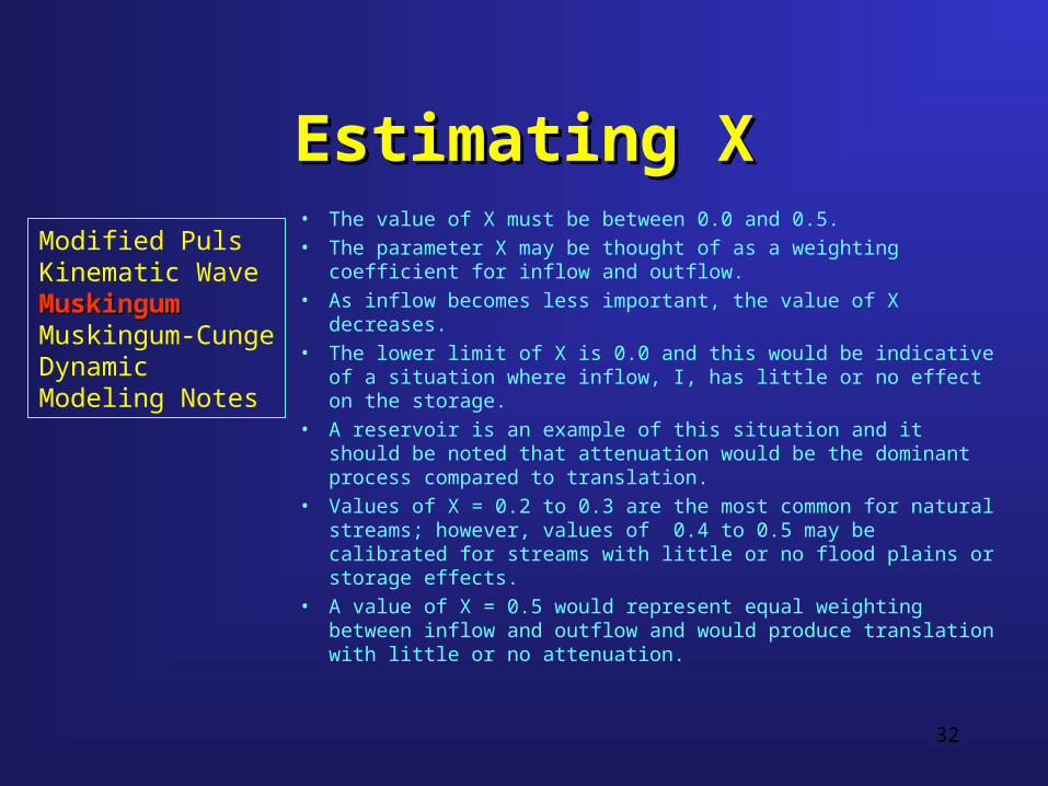
Estimating XEstimating X• The value of X must be between 0.0 and 0.5. • The parameter X may be thought of as a weighting coefficient for
inflow and outflow. • As inflow becomes less important, the value of X decreases. • The lower limit of X is 0.0 and this would be indicative of a
situation where inflow, I, has little or no effect on the storage. • A reservoir is an example of this situation and it should be noted
that attenuation would be the dominant process compared to translation.
• Values of X = 0.2 to 0.3 are the most common for natural streams; however, values of 0.4 to 0.5 may be calibrated for streams with little or no flood plains or storage effects.
• A value of X = 0.5 would represent equal weighting between inflow and outflow and would produce translation with little or no attenuation.
Modified PulsKinematic WaveMuskingumMuskingumMuskingum-CungeDynamicModeling Notes
33
More Notes - MuskingumMore Notes - Muskingum
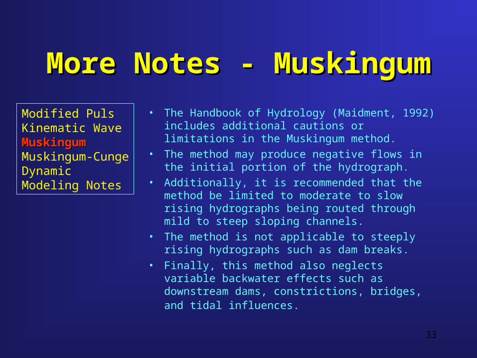
• The Handbook of Hydrology (Maidment, 1992) includes additional cautions or limitations in the Muskingum method.
• The method may produce negative flows in the initial portion of the hydrograph.
• Additionally, it is recommended that the method be limited to moderate to slow rising hydrographs being routed through mild to steep sloping channels.
• The method is not applicable to steeply rising hydrographs such as dam breaks.
• Finally, this method also neglects variable backwater effects such as downstream dams, constrictions, bridges, and tidal influences.
Modified PulsKinematic WaveMuskingumMuskingumMuskingum-CungeDynamicModeling Notes
34
Muskingum Example ProblemMuskingum Example Problem
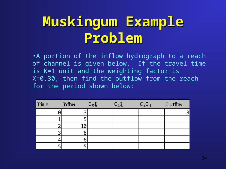
Time Inflow C0I2 C1I1 C2O1 Outflow
0 3 31 52 103 84 65 5
•A portion of the inflow hydrograph to a reach of channel is given below. If the travel time is K=1 unit and the weighting factor is X=0.30, then find the outflow from the reach for the period shown below:
35
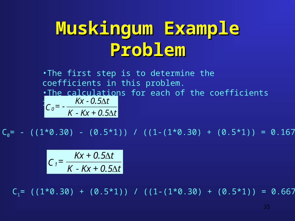
Muskingum Example ProblemMuskingum Example Problem
•The first step is to determine the coefficients in this problem. •The calculations for each of the coefficients is given below:
t0.5 + Kx - K
t0.5 - Kx - = C0
C0= - ((1*0.30) - (0.5*1)) / ((1-(1*0.30) + (0.5*1)) = 0.167
t0.5 + Kx - K
t0.5 + Kx = C1
C1= ((1*0.30) + (0.5*1)) / ((1-(1*0.30) + (0.5*1)) = 0.667
36
Muskingum Example ProblemMuskingum Example Problem
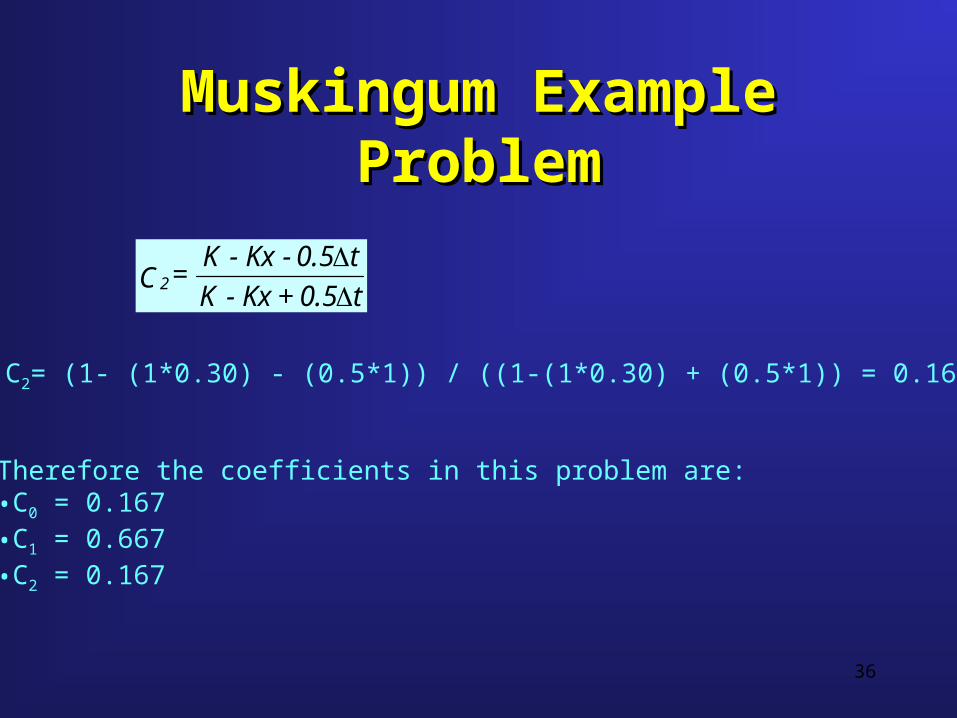
C2= (1- (1*0.30) - (0.5*1)) / ((1-(1*0.30) + (0.5*1)) = 0.167
t0.5 + Kx - K
t0.5 - Kx - K = C2
Therefore the coefficients in this problem are:•C0 = 0.167•C1 = 0.667•C2 = 0.167
37
Muskingum Example ProblemMuskingum Example Problem
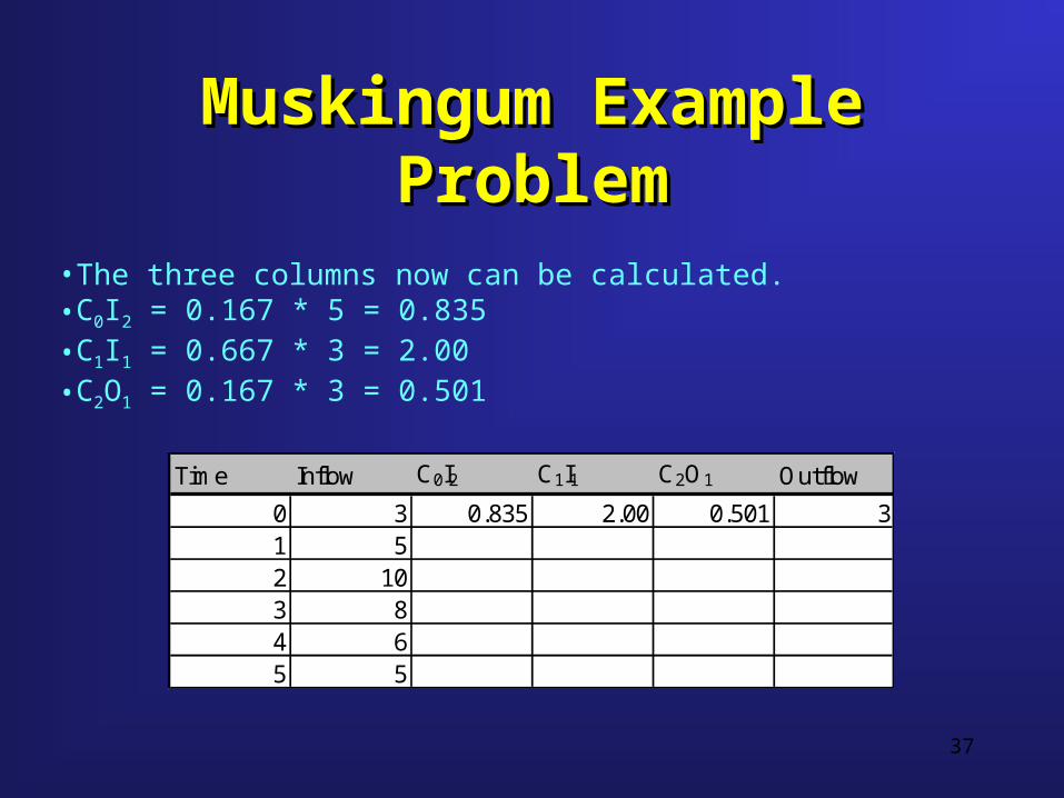
Time Inflow C0I2 C1I1 C2O1 Outflow
0 3 0.835 2.00 0.501 31 52 103 84 65 5
•The three columns now can be calculated.•C0I2 = 0.167 * 5 = 0.835•C1I1 = 0.667 * 3 = 2.00•C2O1 = 0.167 * 3 = 0.501
38
Muskingum Example ProblemMuskingum Example Problem
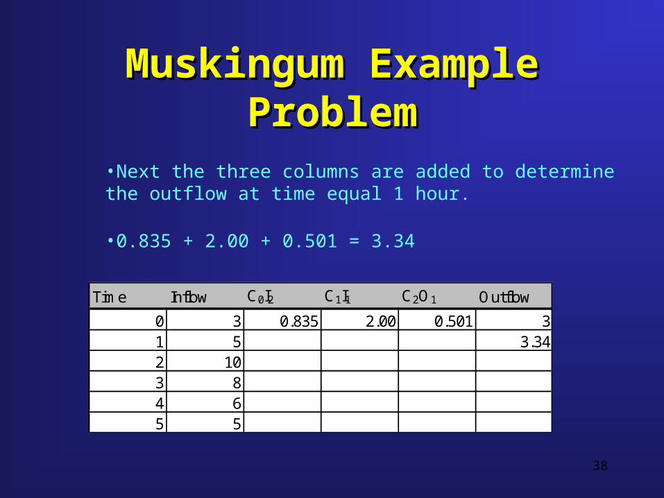
•Next the three columns are added to determine the outflow at time equal 1 hour.
•0.835 + 2.00 + 0.501 = 3.34
Time Inflow C0I2 C1I1 C2O1 Outflow
0 3 0.835 2.00 0.501 31 5 3.342 103 84 65 5
39
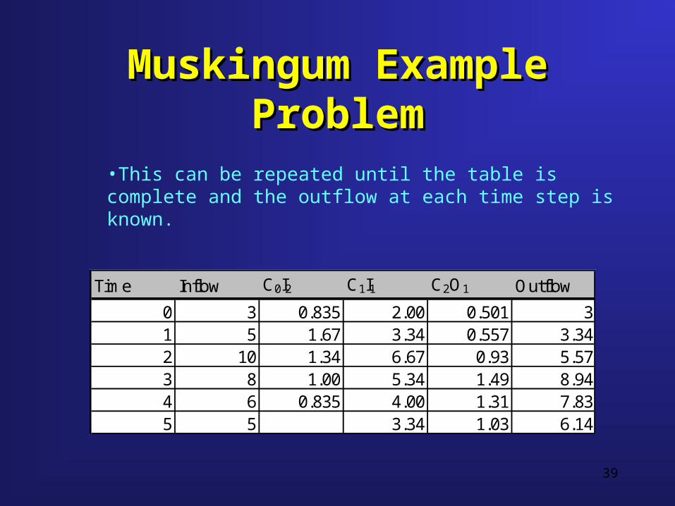
Muskingum Example ProblemMuskingum Example Problem
•This can be repeated until the table is complete and the outflow at each time step is known.
Time Inflow C0I2 C1I1 C2O1 Outflow
0 3 0.835 2.00 0.501 31 5 1.67 3.34 0.557 3.342 10 1.34 6.67 0.93 5.573 8 1.00 5.34 1.49 8.944 6 0.835 4.00 1.31 7.835 5 3.34 1.03 6.14
40
Muskingum-CungeMuskingum-Cunge
• Muskingum-Cunge formulation is similar to the Muskingum type formulation
• The Muskingum-Cunge derivation begins with the continuity equation and includes the diffusion form of the momentum equation.
• These equations are combined and linearized,
Modified PulsKinematic WaveMuskingumMuskingum-CungeMuskingum-CungeDynamicModeling Notes
41
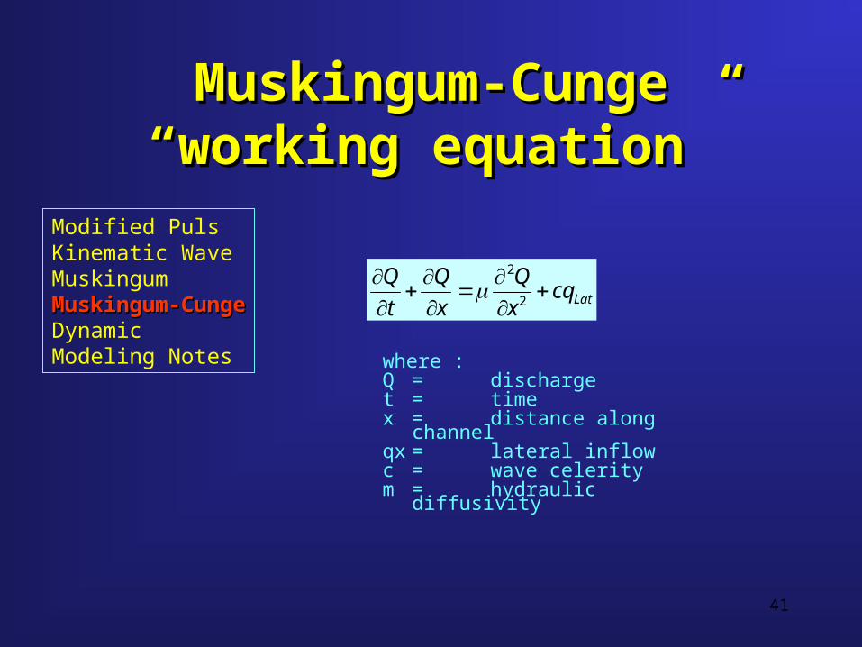
Muskingum-CungeMuskingum-Cunge“working equation”“working equation”
where :Q = discharget = timex = distance along
channelqx = lateral inflowc = wave celeritym = hydraulic diffusivity
Latcqx
Q
x
Q
t
Q
2
2
Modified PulsKinematic WaveMuskingumMuskingum-CungeMuskingum-CungeDynamicModeling Notes
42
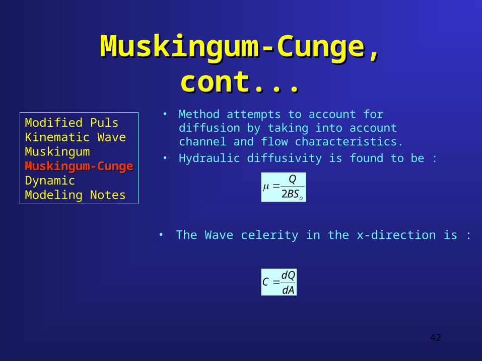
Muskingum-Cunge, cont...Muskingum-Cunge, cont...
• Method attempts to account for diffusion by taking into account channel and flow characteristics.
• Hydraulic diffusivity is found to be :
OBS
Q
2
• The Wave celerity in the x-direction is :
dA
dQC
Modified PulsKinematic WaveMuskingumMuskingum-CungeMuskingum-CungeDynamicModeling Notes
43
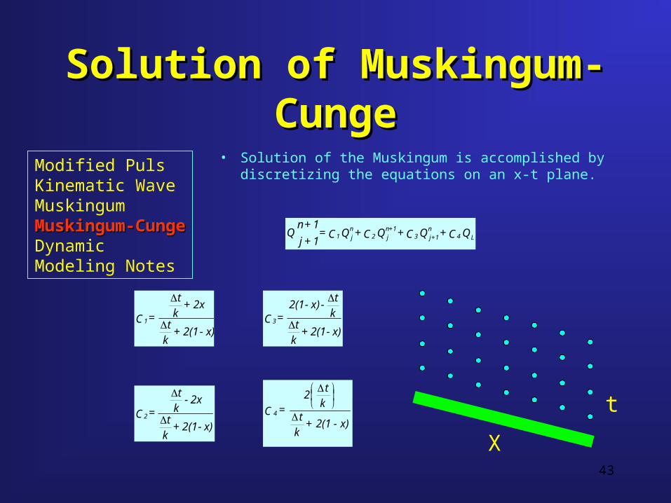
Solution of Muskingum-CungeSolution of Muskingum-Cunge
• Solution of the Muskingum is accomplished by discretizing the equations on an x-t plane.
Q C + Q C + Q C + Q C = 1 +j
1 + n Q L4
n1+j3
1+nj2
nj1
x)-2(1 + kt
2x + kt
= C1
x)-2(1 + kt
2x - kt
= C2
x)-2(1 + kt
kt
-x)-2(1 = C3
x)-2(1 + kt
kt
2 = C 4
X
t
Modified PulsKinematic WaveMuskingumMuskingum-CungeMuskingum-CungeDynamicModeling Notes
44
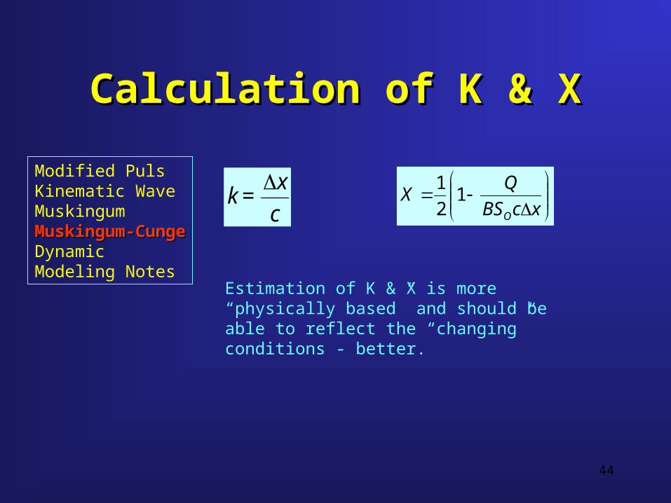
Calculation of K & XCalculation of K & X
c
x = k
xcBS
QX
O
12
1
Estimation of K & X is more “physically based” and should be able to reflect the “changing” conditions - better.
Modified PulsKinematic WaveMuskingumMuskingum-CungeMuskingum-CungeDynamicModeling Notes
45
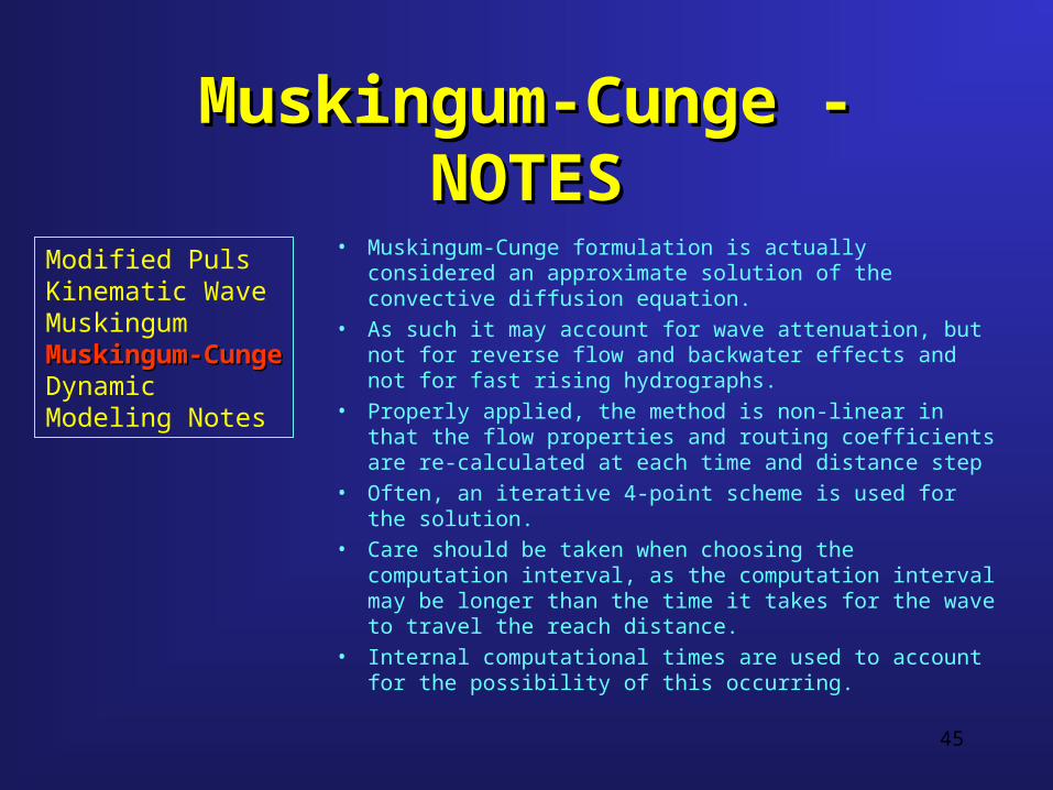
Muskingum-Cunge - NOTESMuskingum-Cunge - NOTES
• Muskingum-Cunge formulation is actually considered an approximate solution of the convective diffusion equation.
• As such it may account for wave attenuation, but not for reverse flow and backwater effects and not for fast rising hydrographs.
• Properly applied, the method is non-linear in that the flow properties and routing coefficients are re-calculated at each time and distance step
• Often, an iterative 4-point scheme is used for the solution.• Care should be taken when choosing the computation
interval, as the computation interval may be longer than the time it takes for the wave to travel the reach distance.
• Internal computational times are used to account for the possibility of this occurring.
Modified PulsKinematic WaveMuskingumMuskingum-CungeMuskingum-CungeDynamicModeling Notes
46
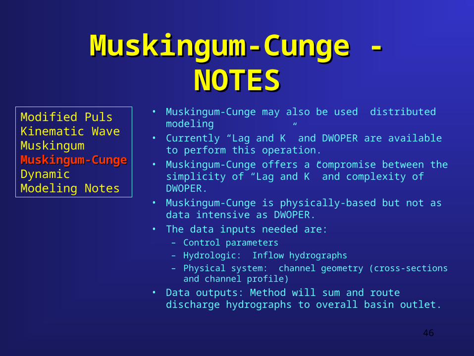
Muskingum-Cunge - NOTESMuskingum-Cunge - NOTES
• Muskingum-Cunge may also be used distributed modeling
• Currently “Lag and K” and DWOPER are available to perform this operation.
• Muskingum-Cunge offers a compromise between the simplicity of “Lag and K” and complexity of DWOPER.
• Muskingum-Cunge is physically-based but not as data intensive as DWOPER.
• The data inputs needed are:– Control parameters– Hydrologic: Inflow hydrographs– Physical system: channel geometry (cross-sections and channel
profile)
• Data outputs: Method will sum and route discharge hydrographs to overall basin outlet.
Modified PulsKinematic WaveMuskingumMuskingum-CungeMuskingum-CungeDynamicModeling Notes
47
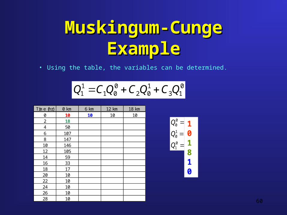
Muskingum-Cunge ExampleMuskingum-Cunge Example
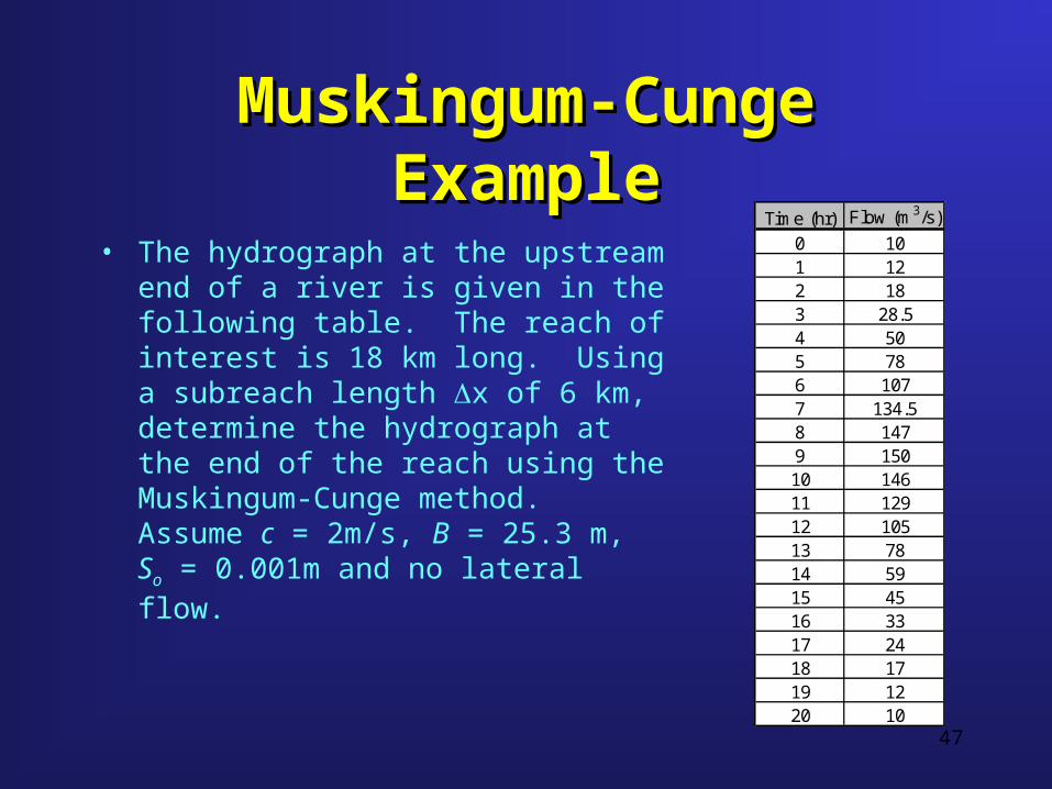
• The hydrograph at the upstream end of a river is given in the following table. The reach of interest is 18 km long. Using a subreach length x of 6 km, determine the hydrograph at the end of the reach using the Muskingum-Cunge method. Assume c = 2m/s, B = 25.3 m, So = 0.001m and no lateral flow.
Time (hr) Flow (m3/s)
0 101 122 183 28.54 505 786 1077 134.58 1479 15010 14611 12912 10513 7814 5915 4516 3317 2418 1719 1220 10
48
Muskingum-Cunge ExampleMuskingum-Cunge Example
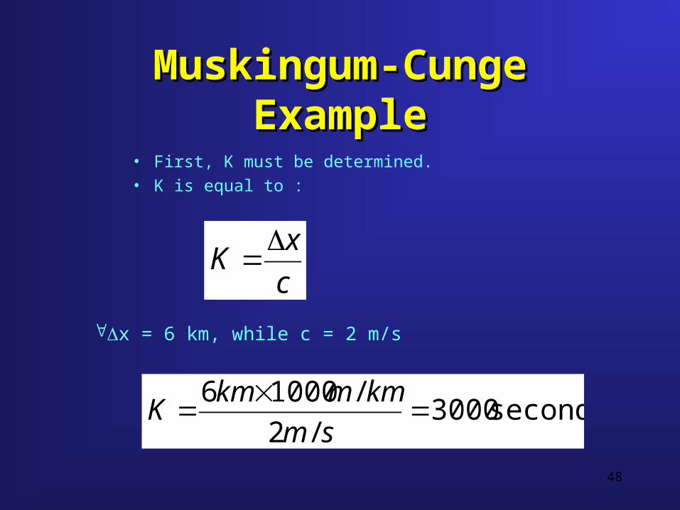
• First, K must be determined.
• K is equal to :
c
xK
seconds3000/2
/10006
sm
kmmkmK
x = 6 km, while c = 2 m/s
49
Muskingum-Cunge ExampleMuskingum-Cunge Example
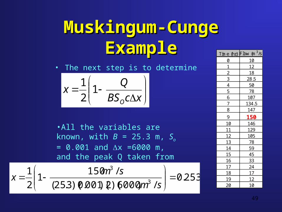
• The next step is to determine x.
xcBS
Qx
O
12
1
•All the variables are known, with B = 25.3 m, So = 0.001 and x =6000 m, and the peak Q taken from the table.
253.0/)6000)(2)(001.0)(3.25(
/1501
2
13
3
sm
smx
Time (hr) Flow (m3/s)
0 101 122 183 28.54 505 786 1077 134.58 147
9 15010 14611 12912 10513 7814 5915 4516 3317 2418 1719 1220 10
50
Muskingum-Cunge ExampleMuskingum-Cunge Example
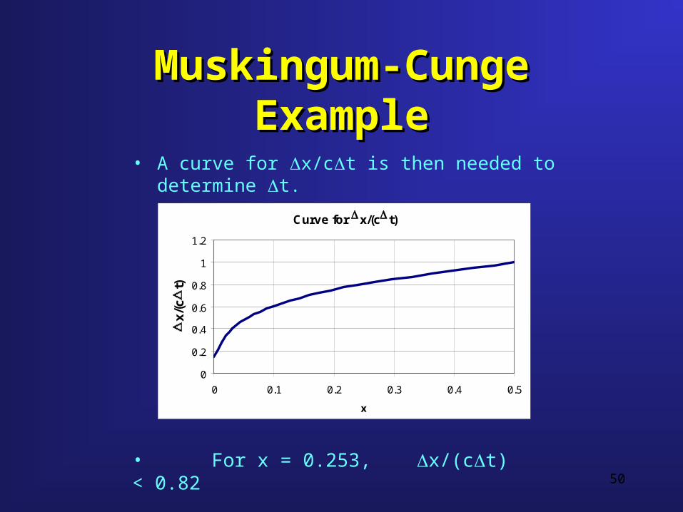
• A curve for x/ct is then needed to determine t.
Curve for x/(c t)
0
0.2
0.4
0.6
0.8
1
1.2
0 0.1 0.2 0.3 0.4 0.5
x
x/(
ct)
• For x = 0.253, x/(ct) < 0.82
51
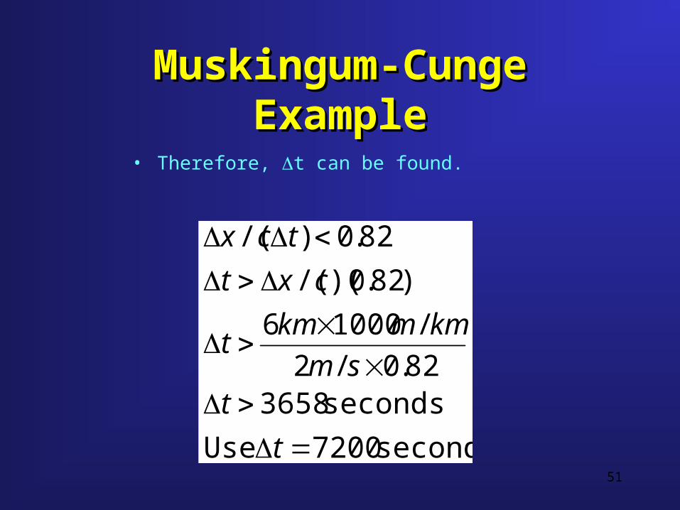
Muskingum-Cunge ExampleMuskingum-Cunge Example
• Therefore, t can be found.
seconds 7200 Use
seconds 365882.0/2
/10006
)82.0)(/(
82.0)/(
t
tsm
kmmkmt
cxt
tcx

52
Muskingum-Cunge ExampleMuskingum-Cunge Example
• The coefficients of the Muskingum-Cunge method can now be determined.
)1(2
2
1
xK
t
xK
t
C
7466.0)253.01(2
30007200
)253.0(230007200
1
C
53
Muskingum-Cunge ExampleMuskingum-Cunge Example
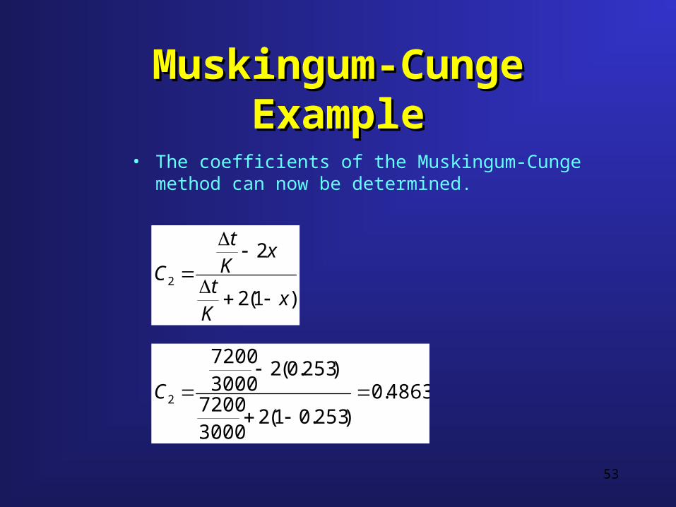
• The coefficients of the Muskingum-Cunge method can now be determined.
)1(2
2
2
xK
t
xK
t
C
4863.0)253.01(2
30007200
)253.0(230007200
2
C
54
Muskingum-Cunge ExampleMuskingum-Cunge Example
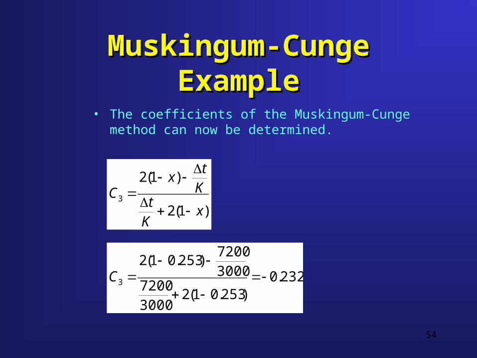
• The coefficients of the Muskingum-Cunge method can now be determined.
)1(2
)1(2
3
xK
tK
tx
C
232.0)253.01(2
30007200
30007200
)253.01(2
3
C
55
Muskingum-Cunge ExampleMuskingum-Cunge Example
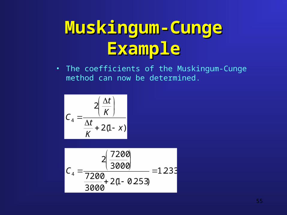
• The coefficients of the Muskingum-Cunge method can now be determined.
)1(2
2
4
xK
tK
t
C
233.1)253.01(2
30007200
30007200
2
4
C
56
Muskingum-Cunge ExampleMuskingum-Cunge Example
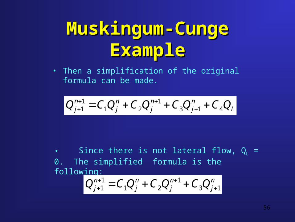
• Then a simplification of the original formula can be made.
Lnj
nj
nj
nj QCQCQCQCQ 413
121
11
• Since there is not lateral flow, QL = 0. The simplified formula is the following:
nj
nj
nj
nj QCQCQCQ 13
121
11
57
Muskingum-Cunge ExampleMuskingum-Cunge Example
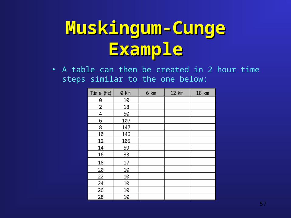
• A table can then be created in 2 hour time steps similar to the one below:
Time (hr) 0 km 6 km 12 km 18 km0 102 184 506 1078 14710 14612 10514 5916 33
18 1720 1022 1024 1026 1028 10
58
Muskingum-Cunge ExampleMuskingum-Cunge Example
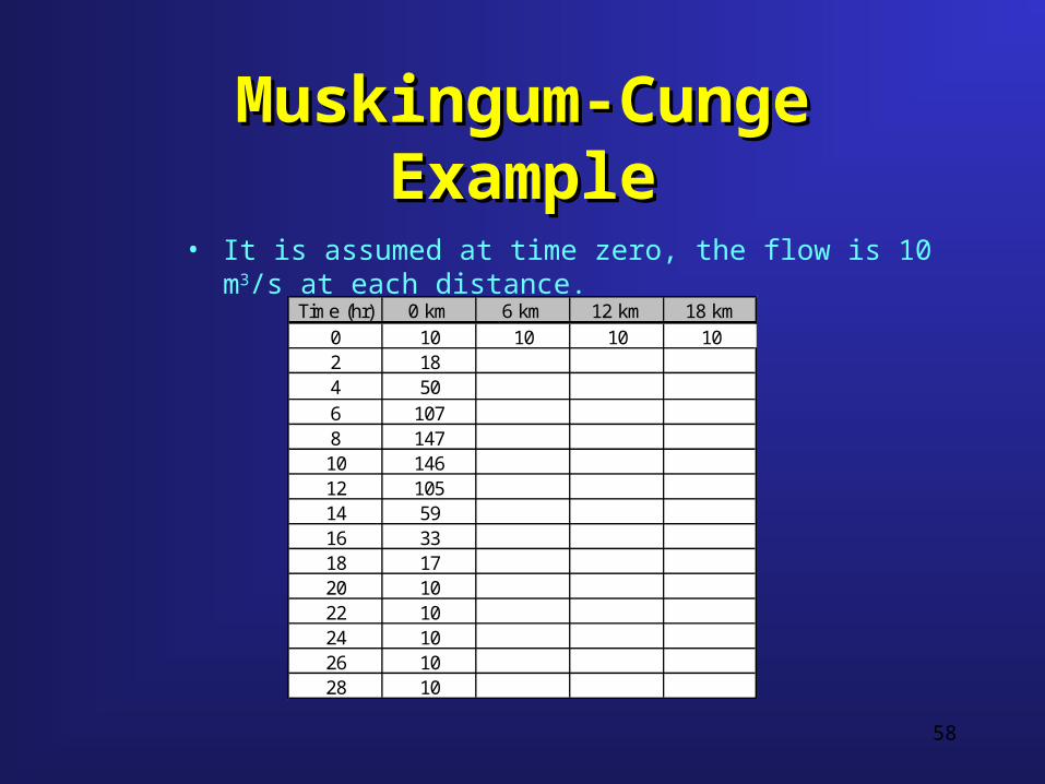
• It is assumed at time zero, the flow is 10 m3/s at each distance.
Time (hr) 0 km 6 km 12 km 18 km0 10 10 10 102 184 506 1078 14710 14612 10514 5916 3318 1720 1022 1024 1026 1028 10
59
Muskingum-Cunge ExampleMuskingum-Cunge Example
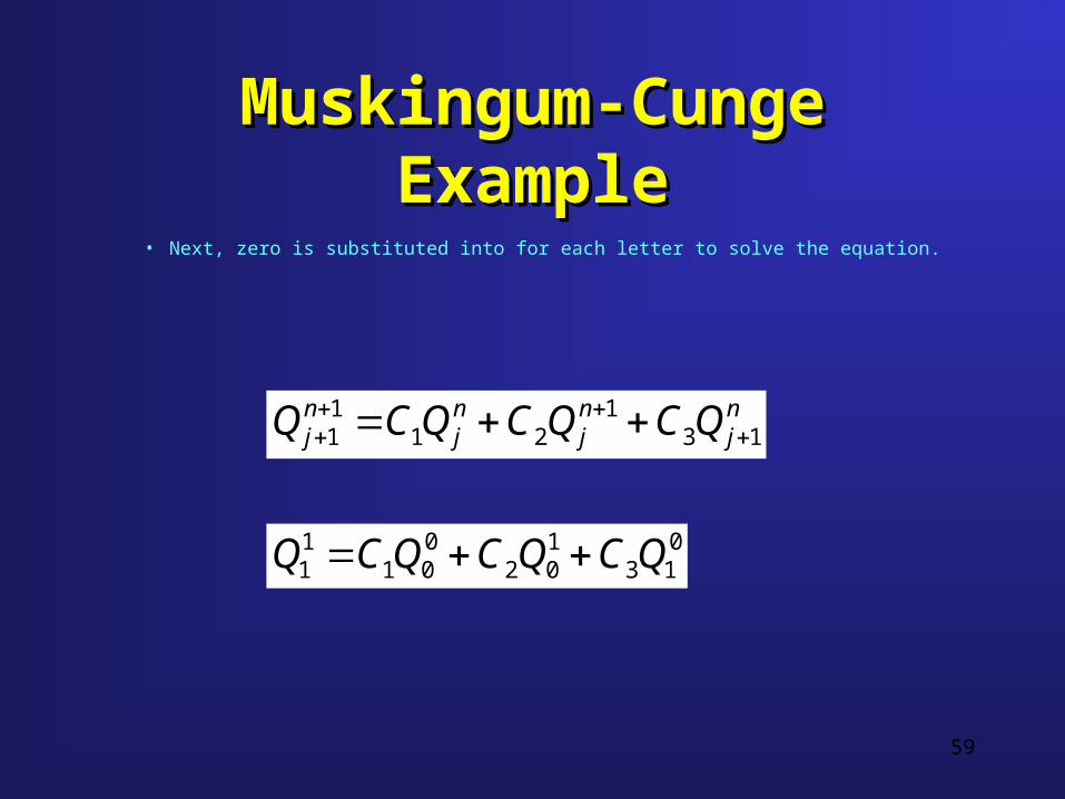
• Next, zero is substituted into for each letter to solve the equation.
nj
nj
nj
nj QCQCQCQ 13
121
11
013
102
001
11 QCQCQCQ
60
Muskingum-Cunge ExampleMuskingum-Cunge Example
• Using the table, the variables can be determined.
013
102
001
11 QCQCQCQ
Time (hr) 0 km 6 km 12 km 18 km0 10 10 10 102 184 506 1078 14710 14612 10514 5916 3318 1720 1022 1024 1026 1028 10
01
10
00
Q
Q
Q 101810
61
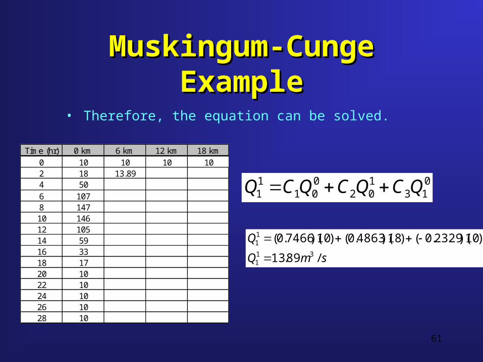
Muskingum-Cunge ExampleMuskingum-Cunge Example
• Therefore, the equation can be solved.
013
102
001
11 QCQCQCQ
smQ
Q
/ 89.13
)10)(2329.0()18)(4863.0()10)(7466.0(31
1
11
Time (hr) 0 km 6 km 12 km 18 km0 10 10 10 102 18 13.894 506 1078 14710 14612 10514 5916 3318 1720 1022 1024 1026 1028 10
62
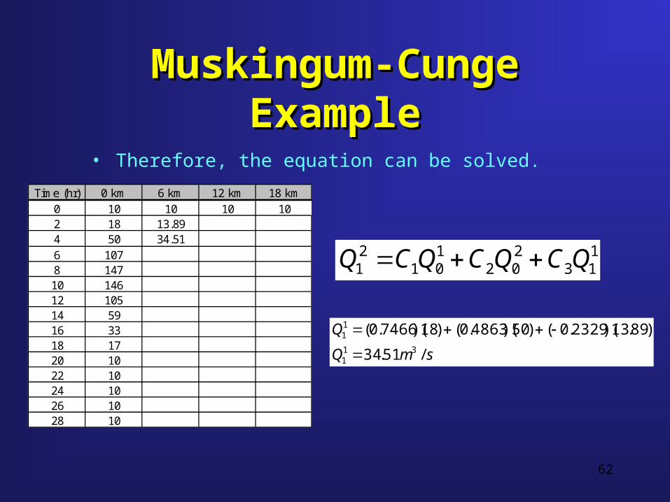
Muskingum-Cunge ExampleMuskingum-Cunge Example
• Therefore, the equation can be solved.
113
202
101
21 QCQCQCQ
smQ
Q
/ 51.34
)89.13)(2329.0()50)(4863.0()18)(7466.0(31
1
11
Time (hr) 0 km 6 km 12 km 18 km0 10 10 10 102 18 13.894 50 34.516 1078 14710 14612 10514 5916 3318 1720 1022 1024 1026 1028 10
63
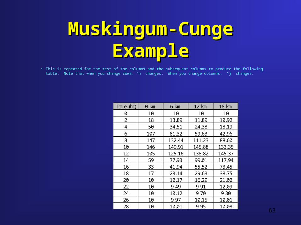
Muskingum-Cunge ExampleMuskingum-Cunge Example• This is repeated for the rest of the columns and the subsequent columns to produce the following table. Note
that when you change rows, “n” changes. When you change columns, “j” changes.
Time (hr) 0 km 6 km 12 km 18 km0 10 10 10 102 18 13.89 11.89 10.924 50 34.51 24.38 18.196 107 81.32 59.63 42.968 147 132.44 111.23 88.6010 146 149.91 145.88 133.3512 105 125.16 138.82 145.3714 59 77.93 99.01 117.9416 33 41.94 55.52 73.4518 17 23.14 29.63 38.7520 10 12.17 16.29 21.0222 10 9.49 9.91 12.0924 10 10.12 9.70 9.3026 10 9.97 10.15 10.0128 10 10.01 9.95 10.08
64
Full Dynamic Wave EquationsFull Dynamic Wave Equations
• The solution of the St. Venant equations is known as dynamic routing.
• Dynamic routing is generally the standard to which other methods are measured or compared.
• The solution of the St. Venant equations is generally accomplished via one of two methods : 1) the method of characteristics and 2) direct methods (implicit and explicit).
• It may be fair to say that regardless of the method of solution, a computer is absolutely necessary as the solutions are quite time consuming.
• J. J. Stoker (1953, 1957) is generally credited for initially attempting to solve the St. Venant equations using a high speed computer.
Modified PulsKinematic WaveMuskingumMuskingum-CungeDynamicDynamicModeling Notes
65
Dynamic Wave SolutionsDynamic Wave Solutions
• Characteristics, Explicit, & Implicit
• The most popular method of applying the implicit technique is to use a four point weighted finite difference scheme.
• Some computer programs utilize a finite element solution technique; however, these tend to be more complex in nature and thus a finite difference technique is most often employed.
• It should be noted that most of the models using the finite difference technique are one-dimensional and that two and three-dimensional solution schemes often revert to a finite element solution.
Modified PulsKinematic WaveMuskingumMuskingum-CungeDynamicDynamicModeling Notes
66
Dynamic Wave SolutionsDynamic Wave Solutions
• Dynamic routing allows for a higher degree of accuracy when modeling flood situations because it includes parameters that other methods neglect.
• Dynamic routing, when compared to other modeling techniques, relies less on previous flood data and more on the physical properties of the storm. This is extremely important when record rainfalls occur or other extreme events.
• Dynamic routing also provides more hydraulic information about the event, which can be used to determine the transportation of sediment along the waterway.
Modified PulsKinematic WaveMuskingumMuskingum-CungeDynamicDynamicModeling Notes
67
Courant Condition?Courant Condition?
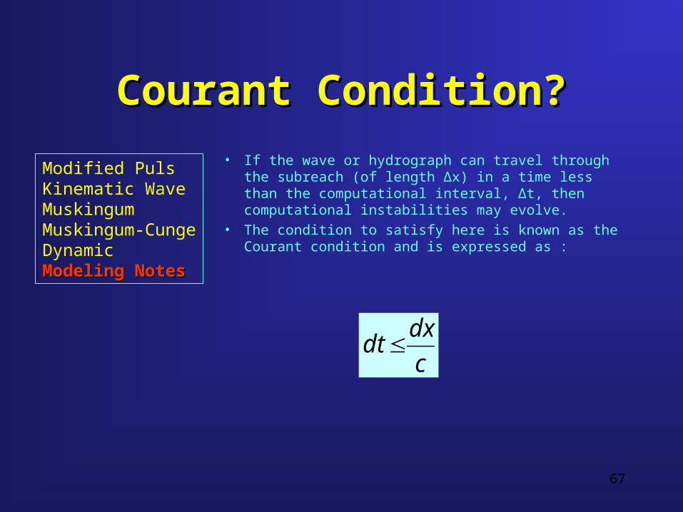
• If the wave or hydrograph can travel through the subreach (of length Δx) in a time less than the computational interval, Δt, then computational instabilities may evolve.
• The condition to satisfy here is known as the Courant condition and is expressed as :
c
dx dt
Modified PulsKinematic WaveMuskingumMuskingum-CungeDynamicModeling NotesModeling Notes
68
Some DISadvantagesSome DISadvantages• Geometric simplification - some models are designed to use very
simplistic representations of the cross-sectional geometry. This may be valid for large dam breaks where very large flows are encountered and width to depth ratios are large; however, this may not be applicable to smaller dam breaks where channel geometry would be more critical.
• Model simulation input requirements - dynamic routing techniques generally require boundary conditions at one or more locations in the domain, such as the upstream and downstream sections. These boundary conditions may in the form of known or constant water surfaces, hydrographs, or assumed stage-discharge relationships.
• Stability - As previously noted, the very complex nature of these methods often leads to numeric instability. Also, convergence may be a problem in some solution schemes. For these reasons as well as others, there tends to be a stability problem in some programs. Often times it is very difficult to obtain a "clean" model run in a cost efficient manner.
Modified PulsKinematic WaveMuskingumMuskingum-CungeDynamicModeling NotesModeling Notes
![YK Channel Routing (1/16)Practical Problems in VLSI Physical Design Yoshimura-Kuh Channel Routing Perform YK channel routing with K = 100 TOP = [1,1,4,2,3,4,3,6,5,8,5,9]](https://img.pdfslide.us/doc/110x75/56649f125503460f94c26664/yk-channel-routing-116practical-problems-in-vlsi-physical-design-yoshimura-kuh.jpg)