Channel Models A Tutorialjain/cse574-08/ftp/channel_model... · Channel Models A Tutorial 1 V1.0 February 21, 2007 Please send comments/corrections/feedback to Raj Jain, [email protected]

Channel Models A Tutorial1

V1.0

February 21, 2007

Please send comments/corrections/feedback to Raj Jain, [email protected]

Please send comments to [email protected]

1 This work was sponsored in part by WiMAX Forum.

Page 2 of 21

V1 Created on 2/21/20072Channel Models: A Tutorial

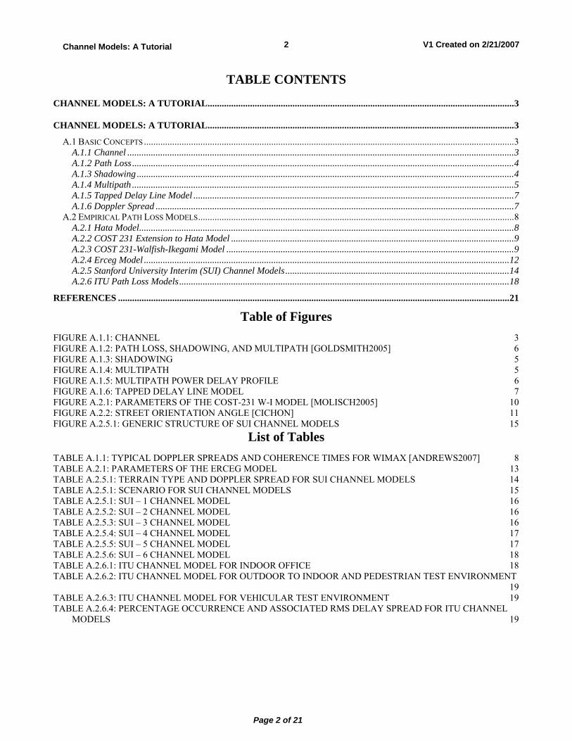
TABLE CONTENTS

CHANNEL MODELS: A TUTORIAL..................................................................................................................................3

CHANNEL MODELS: A TUTORIAL..................................................................................................................................3 A.1 BASIC CONCEPTS .............................................................................................................................................................3

A.1.1 Channel ....................................................................................................................................................................3 A.1.2 Path Loss..................................................................................................................................................................4 A.1.3 Shadowing ................................................................................................................................................................4 A.1.4 Multipath ..................................................................................................................................................................5 A.1.5 Tapped Delay Line Model ........................................................................................................................................7 A.1.6 Doppler Spread ........................................................................................................................................................7

A.2 EMPIRICAL PATH LOSS MODELS......................................................................................................................................8 A.2.1 Hata Model...............................................................................................................................................................8 A.2.2 COST 231 Extension to Hata Model ........................................................................................................................9 A.2.3 COST 231-Walfish-Ikegami Model ..........................................................................................................................9 A.2.4 Erceg Model ...........................................................................................................................................................12 A.2.5 Stanford University Interim (SUI) Channel Models...............................................................................................14 A.2.6 ITU Path Loss Models............................................................................................................................................18

REFERENCES ......................................................................................................................................................................21

Table of Figures FIGURE A.1.1: CHANNEL 3 FIGURE A.1.2: PATH LOSS, SHADOWING, AND MULTIPATH [GOLDSMITH2005] 6 FIGURE A.1.3: SHADOWING 5 FIGURE A.1.4: MULTIPATH 5 FIGURE A.1.5: MULTIPATH POWER DELAY PROFILE 6 FIGURE A.1.6: TAPPED DELAY LINE MODEL 7 FIGURE A.2.1: PARAMETERS OF THE COST-231 W-I MODEL [MOLISCH2005] 10 FIGURE A.2.2: STREET ORIENTATION ANGLE [CICHON] 11 FIGURE A.2.5.1: GENERIC STRUCTURE OF SUI CHANNEL MODELS 15

List of Tables TABLE A.1.1: TYPICAL DOPPLER SPREADS AND COHERENCE TIMES FOR WIMAX [ANDREWS2007] 8 TABLE A.2.1: PARAMETERS OF THE ERCEG MODEL 13 TABLE A.2.5.1: TERRAIN TYPE AND DOPPLER SPREAD FOR SUI CHANNEL MODELS 14 TABLE A.2.5.1: SCENARIO FOR SUI CHANNEL MODELS 15 TABLE A.2.5.1: SUI � 1 CHANNEL MODEL 16 TABLE A.2.5.2: SUI � 2 CHANNEL MODEL 16 TABLE A.2.5.3: SUI � 3 CHANNEL MODEL 16 TABLE A.2.5.4: SUI � 4 CHANNEL MODEL 17 TABLE A.2.5.5: SUI � 5 CHANNEL MODEL 17 TABLE A.2.5.6: SUI � 6 CHANNEL MODEL 18 TABLE A.2.6.1: ITU CHANNEL MODEL FOR INDOOR OFFICE 18 TABLE A.2.6.2: ITU CHANNEL MODEL FOR OUTDOOR TO INDOOR AND PEDESTRIAN TEST ENVIRONMENT

19 TABLE A.2.6.3: ITU CHANNEL MODEL FOR VEHICULAR TEST ENVIRONMENT 19 TABLE A.2.6.4: PERCENTAGE OCCURRENCE AND ASSOCIATED RMS DELAY SPREAD FOR ITU CHANNEL

MODELS 19

Page 3 of 21


A. Channel Models: A Tutorial Many readers may be experts in modeling, programming, or higher layers of networking but may not be familiar with many PHY layer concepts. This tutorial on Channel Models has been designed for such readers. This information has been gathered from various IEEE and ITU standards and contributions and published books.

A.1 Basic Concepts

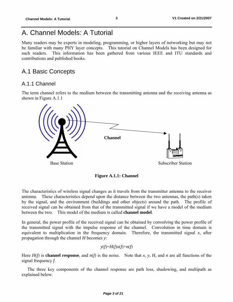
A.1.1 Channel The term channel refers to the medium between the transmitting antenna and the receiving antenna as shown in Figure A.1.1

Channel

Base Station Subscriber Station

Figure A.1.1: Channel

The characteristics of wireless signal changes as it travels from the transmitter antenna to the receiver antenna. These characteristics depend upon the distance between the two antennas, the path(s) taken by the signal, and the environment (buildings and other objects) around the path. The profile of received signal can be obtained from that of the transmitted signal if we have a model of the medium between the two. This model of the medium is called channel model.

In general, the power profile of the received signal can be obtained by convolving the power profile of the transmitted signal with the impulse response of the channel. Convolution in time domain is equivalent to multiplication in the frequency domain. Therefore, the transmitted signal x, after propagation through the channel H becomes y:

y(f)=H(f)x(f)+n(f)

Here H(f) is channel response, and n(f) is the noise. Note that x, y, H, and n are all functions of the signal frequency f.

The three key components of the channel response are path loss, shadowing, and multipath as explained below.

Page 4 of 21


A.1.2 Path Loss

The simplest channel is the free space line of sight channel with no objects between the receiver and the transmitter or around the path between them. In this simple case, the transmitted signal attenuates since the energy is spread spherically around the transmitting antenna. For this line of sight (LOS) channel, the received power is given by:

Pr=Pt ⎣⎢⎡

⎦⎥⎤

Glλ

4πd

2

Here, Pt is the transmitted power, Gl is the product of the transmit and receive antenna field radiation patterns, λ is the wavelength, and d is the distance. Theoretically, the power falls off in proportion to the square of the distance. In practice, the power falls off more quickly, typically 3rd or 4th power of distance.

The presence of ground causes some of the waves to reflect and reach the transmitter. These reflected waves may sometime have a phase shift of 180° and so may reduce the net received power. A simple two-ray approximation for path loss can be shown to be:

2 2

4= t r t rr t

G G h hP Pd

Here, th and rh are the antenna heights of the transmitter and receiver, respectively. Note that there are three major differences from the previous formula. First, the antenna heights have effect. Second, the wavelength is absent and third the exponent on the distance is 4. In general, a common empirical formula for path loss is:

00=r t

dP PPd

α⎛ ⎞⎜ ⎟⎝ ⎠

Where 0P is the power at a distance 0d and α is the path loss exponent. The path loss is given by:

00

( ) ( ) 10 log dPL d dB PL dd

α⎛ ⎞

= + ⎜ ⎟⎝ ⎠

Here 0( )PL d is the mean path loss in dB at distance 0d . The thick dotted line in Figure A.1.2 shows the received power as a function of the distance from the transmitter.

A.1.3 Shadowing

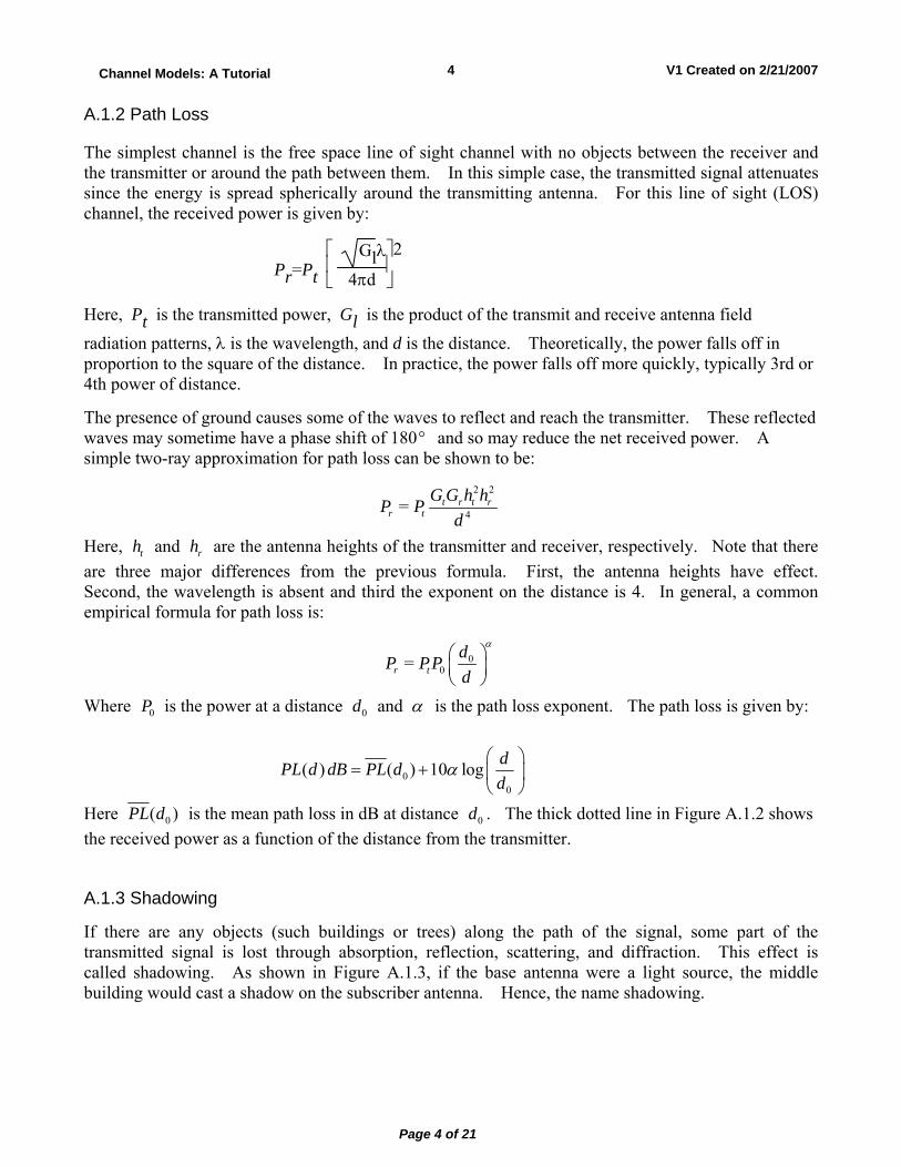
If there are any objects (such buildings or trees) along the path of the signal, some part of the transmitted signal is lost through absorption, reflection, scattering, and diffraction. This effect is called shadowing. As shown in Figure A.1.3, if the base antenna were a light source, the middle building would cast a shadow on the subscriber antenna. Hence, the name shadowing.

Page 5 of 21


Figure A.1.2: Shadowing

The net path loss becomes:

00

( ) ( ) 10 log dPL d dB PL dd

α χ⎛ ⎞

= + +⎜ ⎟⎝ ⎠

Here χ is a normally (Gaussian) distributed random variable (in dB) with standard deviation σ . χ represents the effect of shadowing. As a result of shadowing, power received at the points that are at the same distance d from the transmitter may be different and have a lognormal distribution. This phenomenon is referred to as lognormal shadowing.

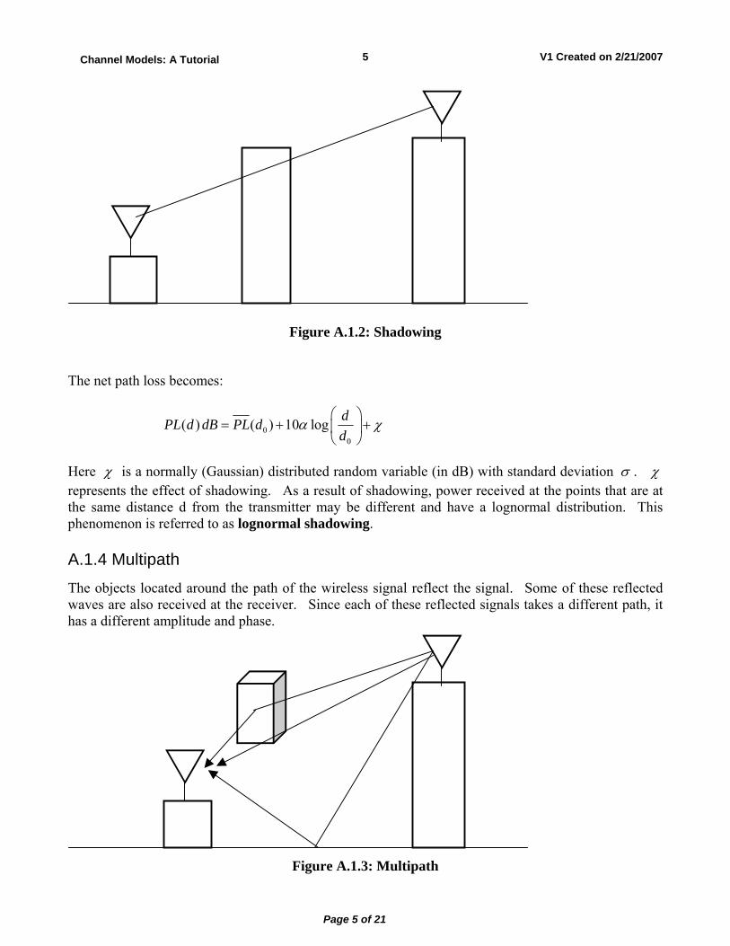
A.1.4 Multipath The objects located around the path of the wireless signal reflect the signal. Some of these reflected waves are also received at the receiver. Since each of these reflected signals takes a different path, it has a different amplitude and phase.

Figure A.1.3: Multipath

Page 6 of 21


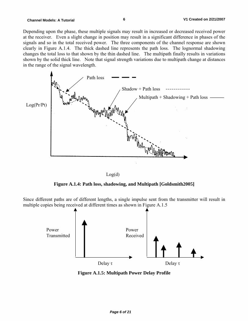
Depending upon the phase, these multiple signals may result in increased or decreased received power at the receiver. Even a slight change in position may result in a significant difference in phases of the signals and so in the total received power. The three components of the channel response are shown clearly in Figure A.1.4. The thick dashed line represents the path loss. The lognormal shadowing changes the total loss to that shown by the thin dashed line. The multipath finally results in variations shown by the solid thick line. Note that signal strength variations due to multipath change at distances in the range of the signal wavelength.

Log(d)

Log(Pr/Pt)

Path loss

Shadow + Path loss

Multipath + Shadowing + Path loss

Figure A.1.4: Path loss, shadowing, and Multipath [Goldsmith2005]

Since different paths are of different lengths, a single impulse sent from the transmitter will result in multiple copies being received at different times as shown in Figure A.1.5

Delay τ

Power Transmitted

Power Received

Delay τ Figure A.1.5: Multipath Power Delay Profile

Page 7 of 21


The maximum delay after which the received signal becomes negligible is called maximum delay spread τmax. A large τmax indicates a highly dispersive channel. Often root-mean-square (rms) value of the delay-spread τrms is used instead of the maximum.

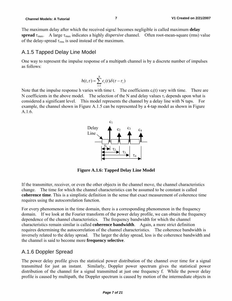
A.1.5 Tapped Delay Line Model One way to represent the impulse response of a multipath channel is by a discrete number of impulses as follows:

1

( , ) ( ) ( )N

i ii

h t c tτ δ τ τ=

= −∑

Note that the impulse response h varies with time t. The coefficients ci(t) vary with time. There are N coefficients in the above model. The selection of the N and delay values τi depends upon what is considered a significant level. This model represents the channel by a delay line with N taps. For example, the channel shown in Figure A.1.5 can be represented by a 4-tap model as shown in Figure A.1.6.

τ1 τ2 τ3 τ4

DelayLine

c1

c2 c3 c4

Figure A.1.6: Tapped Delay Line Model

If the transmitter, receiver, or even the other objects in the channel move, the channel characteristics change. The time for which the channel characteristics can be assumed to be constant is called coherence time. This is a simplistic definition in the sense that exact measurement of coherence time requires using the autocorrelation function.

For every phenomenon in the time domain, there is a corresponding phenomenon in the frequency domain. If we look at the Fourier transform of the power delay profile, we can obtain the frequency dependence of the channel characteristics. The frequency bandwidth for which the channel characteristics remain similar is called coherence bandwidth. Again, a more strict definition requires determining the autocorrelation of the channel characteristics. The coherence bandwidth is inversely related to the delay spread. The larger the delay spread, less is the coherence bandwidth and the channel is said to become more frequency selective.

A.1.6 Doppler Spread The power delay profile gives the statistical power distribution of the channel over time for a signal transmitted for just an instant. Similarly, Doppler power spectrum gives the statistical power distribution of the channel for a signal transmitted at just one frequency f. While the power delay profile is caused by multipath, the Doppler spectrum is caused by motion of the intermediate objects in

Page 8 of 21


the channel. The Doppler power spectrum is nonzero for (f-fD, f+fD), where fD is the maximum Doppler spread or Doppler spread.

The coherence time and Doppler spread are inversely related:

1CoherenceTime

Doppler Spread≈

Thus, if the transmitter, receiver, or the intermediate objects move very fast, the Doppler spread is large and the coherence time is small, i.e., the channel changes fast.

Table A.1.1 lists typical values for the Doppler spread and associated channel coherence time for two WiMAX frequency bands. Note that at high mobility, the channel changes 500 times per second, requiring good channel estimation algorithms

Table A.1.1: Typical Doppler Spreads and Coherence Times for WiMAX [Andrews2007]

Carrier Freq Speed Max Doppler Spread Coherence Time 2.5 GHz 2 km/hr 4.6 Hz 200 ms 2.5 GHz 45 km/hr 104.2 Hz 10 ms 2.5 GHz 100 km/hr 231.5 Hz 4 ms 5.8 GHz 2 km/hr 10.7 Hz 93 ms 5.8 GHz 45 km/hr 241.7 Hz 4 ms 5.8 GHz 100 km/hr 537 Hz 2 ms

A.2 Empirical Path Loss Models Actual environments are too complex to model accurately. In practice, most simulation studies use empirical models that have been developed based on measurements taken in various real environments. In this section we describe a number of commonly used empirical models.

A.2.1 Hata Model

In 1968, Okumura conducted extensive measurements of base station to mobile signal attenuation throughout Tokyo and developed a set of curves giving median attenuation relative to free space path loss. To use this model one needs to use the empirical plots given in his paper. This is not very convenient to use. So in 1980, Hata developed closed-form expressions for Okumura's data. According to Hata model the path loss in an urban area at a distance d is:

, 1 1 1 1( ) = 69.55 26.16 0( ) 13.82 0( ) ( ) (44.9 6.55 0( )) 0( )log log log logL urban c t r tP d dB f h a h h d+ − − + −

Here, cf is the carrier frequency, th is the height of the transmitting (base station) antenna, rh is the height of the receiving (mobile) antenna, and ( )ra h is a correction factor for the mobile antenna height based on the size of the coverage area.

Page 9 of 21


Hata model well approximates the Okumura model for distances greater than 1km. This model is intended for large cells with BS being placed higher than the surrounding rooftops. Both models are designed for 150-1500 MHz and are applicable to the first generation cellular systems. They may not work well for WiMAX systems with smaller cell sizes and higher frequencies.

A.2.2 COST 231 Extension to Hata Model

The European Cooperative for Scientific and Technical (COST) research extended the Hata model to 2 GHz as follows:

, 10 10 10 10( ) = 46.3 33.9 ( ) 13.82 ( ) ( ) (44.9 6.55 ( )) ( )log log log logL urban c t r t MP d dB f h a h h d C+ − − + − +

Here, MC is 0 dB for medium sized cities and suburbs and is 3 dB for metropolitan areas. The remaining parameters are same as before. This model is restricted to the following range of parameters:

Carrier Frequency 1.5 GHz to 2 GHz

Base Antenna Height 30 m to 300 m

Mobile Antenna Height 1m to 10 m

Distance d 1 km to 20 km

COST 321-Hata model is designed for large and small macro-cells, i.e., base station antenna heights above rooftop levels adjacent to base station.

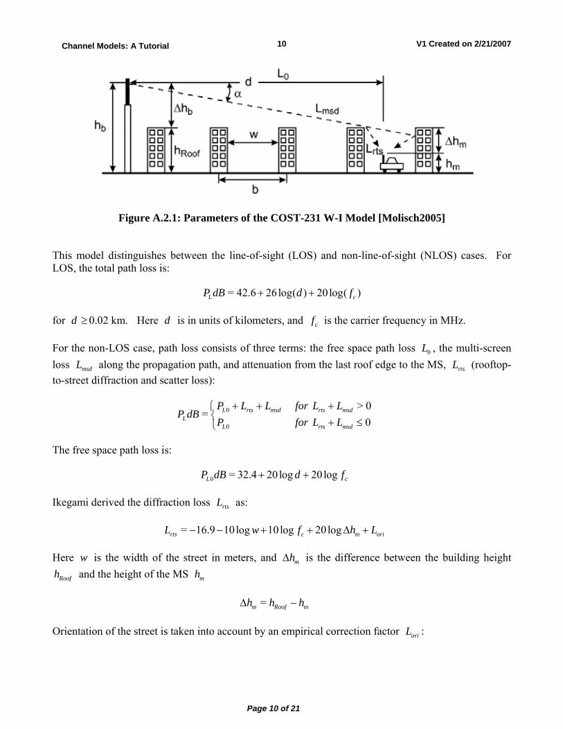
A.2.3 COST 231-Walfish-Ikegami Model

In addition to the COST 231-Hata model, the COST 231 group also proposed another model for micro cells and small macro cells by combining models proposed by Walfisch and Ikegami [Walfisch1988]. This model considers additional characteristics of the urban environment, namely, heights of buildings

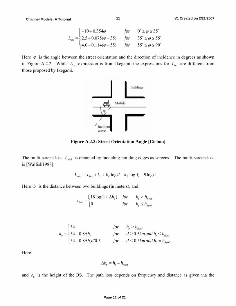
roofh , width of roads w , building separation b , and road orientation with respect to the direct radio path ϕ . These parameters are shown in Figure A.2.1 below.

Page 10 of 21


Figure A.2.1: Parameters of the COST-231 W-I Model [Molisch2005]

This model distinguishes between the line-of-sight (LOS) and non-line-of-sight (NLOS) cases. For LOS, the total path loss is:

= 42.6 26log( ) 20log( )L cP dB d f+ +

for d ≥ 0.02 km. Here d is in units of kilometers, and cf is the carrier frequency in MHz.

For the non-LOS case, path loss consists of three terms: the free space path loss 0L , the multi-screen loss msdL along the propagation path, and attenuation from the last roof edge to the MS, rtsL (rooftop-to-street diffraction and scatter loss):

0

0

> 0=

0L rts msd rts msd

LL rts msd

P L L for L LP dB

P for L L+ + +⎧

⎨ + ≤⎩

The free space path loss is:

0 = 32.4 20log 20logL cP dB d f+ +

Ikegami derived the diffraction loss rtsL as:

= 16.9 10log 10log 20logrts c m oriL w f h L− − + + Δ +

Here w is the width of the street in meters, and mhΔ is the difference between the building height

Roofh and the height of the MS mh

=m Roof mh h hΔ −

Orientation of the street is taken into account by an empirical correction factor oriL :

Page 11 of 21


10 0.354 0 35

= 2.5 0.075( 35) 35 554.0 0.114( 55) 55 90

ori

forL for

for

ϕ ϕϕ ϕϕ ϕ

⎧− + ≤ ≤⎪ + − ≤ ≤⎨⎪ − − ≤ ≤⎩

o o

o o

o o

Here ϕ is the angle between the street orientation and the direction of incidence in degrees as shown in Figure A.2.2. While rtsL expression is from Ikegami, the expressions for oriL are different from those proposed by Ikegami.

Figure A.2.2: Street Orientation Angle [Cichon]

The multi-screen loss msdL is obtained by modeling building edges as screens. The multi-screen loss is [Walfish1988]:

= log log 9logmsd bsh a d f cL L k k d k f b+ + + −

Here b is the distance between two buildings (in meters), and:

18log(1 ) >

=0

b b Roofbsh

b Roof

h for h hL

for h h+ Δ⎧

⎨ ≤⎩

54 >

= 54 0.8 0.554 0.8 /0.5 < 0.5

b Roof

a b b Roof

b b Roof

for h hk h for d km and h h

h d for d km and h h

⎧⎪ − Δ ≥ ≤⎨⎪ − Δ =⎩

Here

=b b Roofh h hΔ −

and bh is the height of the BS. The path loss depends on frequency and distance as given via the

Page 12 of 21


parameters dk and fk :

18 >

=18 15 /

b Roofd

b Roof b Roof

for h hk

h h for h h⎧⎨ − Δ ≤⎩

0.7 1925

=

1.5 1925

c

f

c

f for medium sizecities

k suburban areas with averagevegetation densityf for metropolitan areas

⎧ ⎛ ⎞− −⎜ ⎟⎪ ⎝ ⎠⎪⎪⎨⎪ ⎛ ⎞⎪ −⎜ ⎟⎪ ⎝ ⎠⎩

The validity range for this model is:

Carrier frequency cf 800�2,000 MHz

Height of BS antenna bh 4�50m

Height of MS antenna mh 1�3m

Distance d 0.02�5km

The model assumes a Manhattan street grid (streets intersecting at right angles), constant building height, and flat terrain. The model does not include the effect of wave guiding through street canyons, which can lead to an underestimation of the received field strength.

The COST 231-WI model has been accepted by ITU-R and is included in Report 567-4. The estimation of the path loss agrees well with measurements for base station antenna heights above rooftop level. The prediction error becomes large for Baseh = Roofh compared to situations where

Base Roofh h! . Also, the performance of the model is poor for Base Roofh h" . The prediction error for micro-cells may be quite large. The reliability of the estimation decreases also if terrain is not flat or the land cover is inhomogeneous.

A.2.4 Erceg Model

This model [Erceg1999] is based on extensive experimental data collected by AT&T Wireless Services across the United States in 95 existing macro cells at 1.9GHz. The terrains are classified in three categories. Category A is hilly terrain with moderate-to-heavy tree density and has a high path loss. Category C is mostly flat terrain with light tree density and has a low path loss. Category B is hilly

Page 13 of 21


terrain with light tree density or flat terrain with moderate-to-heavy tree density. Category B has an intermediate path loss. For all three categories, the median path loss at distance 0>d d is given by:

0 0 010 10= 20 (4 / ) 10 ( / ) >log logLP dB d d d s for d dπ λ γ+ +

Here, λ is the wavelength in meters, γ is the path-loss exponent with:

= /b ba bh d hγ − +

bh is the height of the base station in meters (between 10 m and 80 m), 0d = 100 m, and a, b, c are constants dependent on the terrain category. These parameters are listed in the table below.

Table A.2.1: Parameters of the Erceg Model

Model Parameter Terrain Type A Terrain Type B Terrain Type C

a 4.6 4 3.6

b 0.0075 0.0065 0.005

c 12.6 17.1 20

s represents the shadowing effect and follows a lognormal distribution with a typical standard deviation of 8.2 to 10.6 dB.

The above model is valid for frequencies close to 2 GHz and for receive antenna heights close to 2 m. For other frequencies and antenna heights (between 2 m and 10 m), the following correction terms are recommended [Molisch2005]:

=modified f hPL PL PL PL+ Δ + Δ

Here, PL, is the path loss given earlier, fPLΔ is the frequency term, and hPLΔ is the receive antenna height correction terms given as follows:

10= 6 ( /2000)logfPL fΔ

10

10

10.8 ( /2)log=

20 ( /2)logh

h for Categories Aand BPL

h for Category C−⎧

Δ ⎨−⎩

Page 14 of 21


A.2.5 Stanford University Interim (SUI) Channel Models

This is a set of 6 channel models representing three terrain types and a variety of Doppler spreads, delay spread and line-of-sight/non-line-of-site conditions that are typical of the continental US as follows[Erceg2001]:

Table A.2.5.1: Terrain Type and Doppler Spread for SUI Channel Models

Channel Terrain Type Doppler Spread

Spread LOS

SUI-1 C Low Low High

SUI-2 C Low Low High

SUI-3 B Low Low Low

SUI-4 B High Moderate Low

SUI-5 A Low High Low

SUI-6 A High High Low

The terrain type A, B,C are same as those defined earlier for Erceg model. The multipath fading is modeled as a tapped delay line with 3 taps with non-uniform delays. The gain associated with each tap is characterized by a Rician Distribution and the maximum Doppler frequency.

In a multipath environment, the received power r has a Rician distribution, whose pdf is given by:

[ ]2 2 2

02 2

2( ) = 0

fracr Ar rApdf r e I rσ

σ σ− + ⎛ ⎞ ≤ ≤ ∞⎜ ⎟

⎝ ⎠

Here, 0 ( )I x is the modified Bessel function of the first kind, zero order. A is zero if there is no LOS component and the pdf of the received power becomes:

2

2

22( ) = 0

rrpdf r e rσ

σ

−⎡ ⎤⎣ ⎦ ≤ ≤ ∞

This is the Raleigh distribution. The ratio 2 2= /(2 )K A σ in the Rician case represents the ratio of LOS component to NLOS component and is called the "K-Factor" or "Rician Factor." For NLOS case, K-factor is zero and the Rician distribution reduces to Raleigh Distribution.

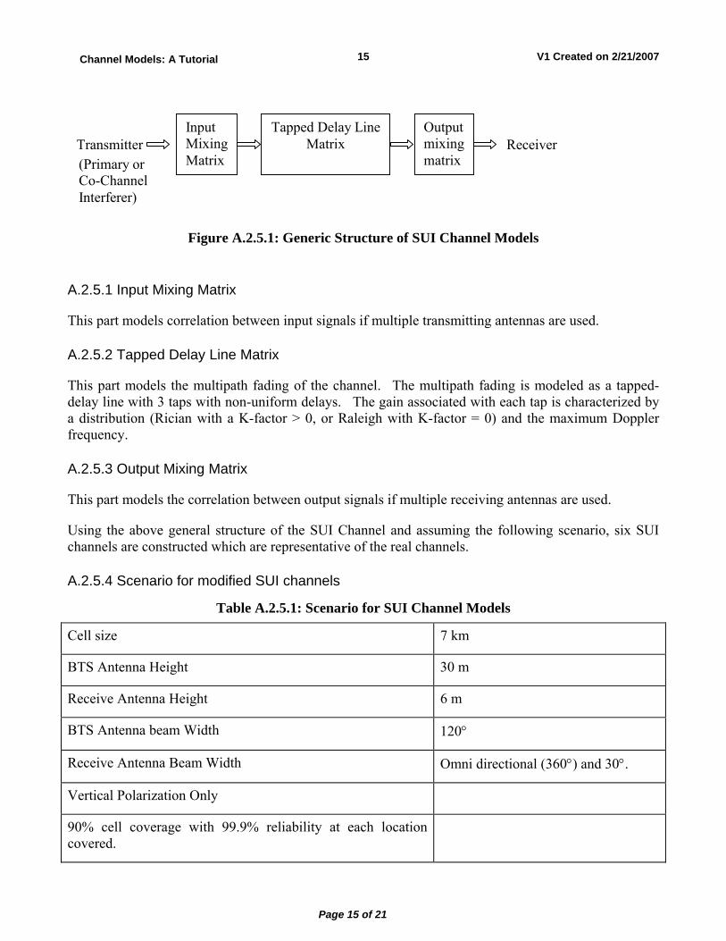
The general structure for the SUI channel model is as shown below in Figure A.2.5.1. This structure is for Multiple Input Multiple Output (MIMO) channels and includes other configurations like Single Input Single Output (SISO) and Single Input Multiple Output (SIMO) as subsets. The SUI channel structure is the same for the primary and interfering signals.

Page 15 of 21


Transmitter

Input MixingMatrix

Tapped Delay LineMatrix

Outputmixingmatrix

Receiver (Primary or Co-Channel Interferer)

Figure A.2.5.1: Generic Structure of SUI Channel Models

A.2.5.1 Input Mixing Matrix

This part models correlation between input signals if multiple transmitting antennas are used.

A.2.5.2 Tapped Delay Line Matrix

This part models the multipath fading of the channel. The multipath fading is modeled as a tapped-delay line with 3 taps with non-uniform delays. The gain associated with each tap is characterized by a distribution (Rician with a K-factor > 0, or Raleigh with K-factor = 0) and the maximum Doppler frequency.

A.2.5.3 Output Mixing Matrix

This part models the correlation between output signals if multiple receiving antennas are used.

Using the above general structure of the SUI Channel and assuming the following scenario, six SUI channels are constructed which are representative of the real channels.

A.2.5.4 Scenario for modified SUI channels

Table A.2.5.1: Scenario for SUI Channel Models

Cell size 7 km

BTS Antenna Height 30 m

Receive Antenna Height 6 m

BTS Antenna beam Width 120°

Receive Antenna Beam Width Omni directional (360°) and 30°.

Vertical Polarization Only

90% cell coverage with 99.9% reliability at each location covered.

Page 16 of 21


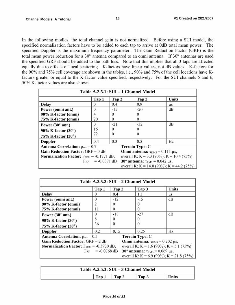
In the following modles, the total channel gain is not normalized. Before using a SUI model, the specified normalization factors have to be added to each tap to arrive at 0dB total mean power. The specified Doppler is the maximum frequency parameter. The Gain Reduction Factor (GRF) is the total mean power reduction for a 30° antenna compared to an omni antenna. If 30° antennas are used the specified GRF should be added to the path loss. Note that this implies that all 3 taps are affected equally due to effects of local scattering. K-factors have linear values, not dB values. K-factors for the 90% and 75% cell coverage are shown in the tables, i.e., 90% and 75% of the cell locations have K-factors greater or equal to the K-factor value specified, respectively. For the SUI channels 5 and 6, 50% K-factor values are also shown.

Table A.2.5.1: SUI – 1 Channel Model Tap 1 Tap 2 Tap 3 Units Delay 0 0.4 0.9 µs Power (omni ant.) 90% K-factor (omni) 75% K-factor (omni)

0 4 20

-15 0 0

-20 0 0

dB

Power (30° ant.) 90% K-factor (30°) 75% K-factor (30°)

0 16 72

-21 0 0

-32 0 0

dB

Doppler 0.4 0.3 0.5 Hz Antenna Correlation: ρENV = 0.7 Gain Reduction Factor: GRF = 0 dB Normalization Factor: Fomni = -0.1771 dB, F30° = -0.0371 dB

Terrain Type: C Omni antenna: τRMS = 0.111 µs, overall K: K = 3.3 (90%); K = 10.4 (75%) 30° antenna: τRMS = 0.042 µs, overall K: K = 14.0 (90%); K = 44.2 (75%)

Table A.2.5.2: SUI – 2 Channel Model Tap 1 Tap 2 Tap 3 Units Delay 0 0.4 1.1 µs Power (omni ant.) 90% K-factor (omni) 75% K-factor (omni)

0 2 11

-12 0 0

-15 0 0

dB


0 8 36

-18 0 0

-27 0 0

dB


Terrain Type: C Omni antenna: τRMS = 0.202 µs, overall K: K = 1.6 (90%); K = 5.1 (75%) 30° antenna: τRMS = 0.069 µs, overall K: K = 6.9 (90%); K = 21.8 (75%)

Table A.2.5.3: SUI – 3 Channel Model Tap 1 Tap 2 Tap 3 Units

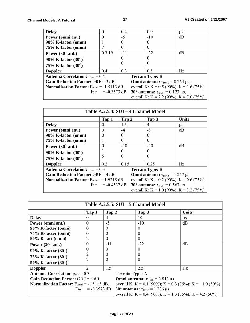
Page 17 of 21


Delay 0 0.4 0.9 µs Power (omni ant.) 90% K-factor (omni) 75% K-factor (omni)

0 1 7

-5 0 0

-10 0 0

dB


0 3 19 -11 0 0

-22 0 0

dB


Terrain Type: B Omni antenna: τRMS = 0.264 µs, overall K: K = 0.5 (90%); K = 1.6 (75%) 30° antenna: τRMS = 0.123 µs, overall K: K = 2.2 (90%); K = 7.0 (75%)

Table A.2.5.4: SUI – 4 Channel Model Tap 1 Tap 2 Tap 3 Units Delay 0 1.5 4 µs Power (omni ant.) 90% K-factor (omni) 75% K-factor (omni)

0 0 1

-4 0 0

-8 0 0

dB


0 1 5

-10 0 0

-20 0 0

dB


Terrain Type: B Omni antenna: τRMS = 1.257 µs overall K: K = 0.2 (90%); K = 0.6 (75%) 30° antenna: τRMS = 0.563 µs overall K: K = 1.0 (90%); K = 3.2 (75%)

Table A.2.5.5: SUI – 5 Channel Model Tap 1 Tap 2 Tap 3 Units Delay 0 4 10 µs Power (omni ant.) 90% K-factor (omni) 75% K-factor (omni) 50% K-fact (omni)

0 0 0 2

-5 0 0 0

-10 0 0 0

dB

Power (30° ant.) 90% K-factor (30°) 75% K-factor (30°) 50% K-factor (30°)

0 0 2 7

-11 0 0 0

-22 0 0 0

dB

Doppler 2 1.5 2.5 Hz Antenna Correlation: ρENV = 0.3 Gain Reduction Factor: GRF = 4 dB Normalization Factor: Fomni = -1.5113 dB, F30° = -0.3573 dB

Terrain Type: A Omni antenna: τRMS = 2.842 µs overall K: K = 0.1 (90%); K = 0.3 (75%); K = 1.0 (50%) 30° antenna: τRMS = 1.276 µs overall K: K = 0.4 (90%); K = 1.3 (75%); K = 4.2 (50%)

Page 18 of 21


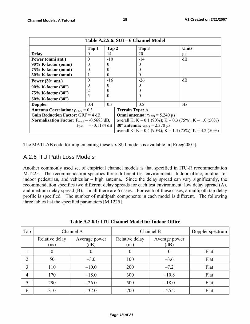
Table A.2.5.6: SUI – 6 Channel Model Tap 1 Tap 2 Tap 3 Units Delay 0 14 20 µs Power (omni ant.) 90% K-factor (omni) 75% K-factor (omni) 50% K-factor (omni)

0 0 0 1

-10 0 0 0

-14 0 0 0

dB

Power (30° ant.) 90% K-factor (30°) 75% K-factor (30°) 50% K-factor (30°)

0 0 2 5

-16 0 0 0

-26 0 0 0

dB


Terrain Type: A Omni antenna: τRMS = 5.240 µs overall K: K = 0.1 (90%); K = 0.3 (75%); K = 1.0 (50%) 30° antenna: τRMS = 2.370 µs overall K: K = 0.4 (90%); K = 1.3 (75%); K = 4.2 (50%)

The MATLAB code for implementing these six SUI models is available in [Erceg2001].

A.2.6 ITU Path Loss Models

Another commonly used set of empirical channel models is that specified in ITU-R recommendation M.1225. The recommendation specifies three different test environments: Indoor office, outdoor-to-indoor pedestrian, and vehicular � high antenna. Since the delay spread can vary significantly, the recommendation specifies two different delay spreads for each test environment: low delay spread (A), and medium delay spread (B). In all there are 6 cases. For each of these cases, a multipath tap delay profile is specified. The number of multipath components in each model is different. The following three tables list the specified parameters [M.1225].

Table A.2.6.1: ITU Channel Model for Indoor Office

Tap Channel A Channel B Doppler spectrum

Relative delay (ns)

Average power (dB)

Relative delay (ns)

Average power (dB)

1 0 0 0 0 Flat 2 50 �3.0 100 �3.6 Flat 3 110 �10.0 200 �7.2 Flat 4 170 �18.0 300 �10.8 Flat 5 290 �26.0 500 �18.0 Flat 6 310 �32.0 700 �25.2 Flat

Page 19 of 21


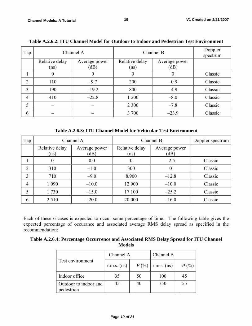
Table A.2.6.2: ITU Channel Model for Outdoor to Indoor and Pedestrian Test Environment


Relative delay (ns)

Average power (dB)

Relative delay (ns)

Average power (dB)

1 0 0 0 0 Classic 2 110 �9.7 200 �0.9 Classic 3 190 �19.2 800 �4.9 Classic 4 410 �22.8 1 200 �8.0 Classic 5 � � 2 300 �7.8 Classic 6 � � 3 700 �23.9 Classic

Table A.2.6.3: ITU Channel Model for Vehicular Test Environment


Relative delay (ns)

Average power (dB)

Relative delay (ns)

Average power (dB)

1 0 0.0 0 �2.5 Classic 2 310 �1.0 300 0 Classic 3 710 �9.0 8.900 �12.8 Classic 4 1 090 �10.0 12 900 �10.0 Classic 5 1 730 �15.0 17 100 �25.2 Classic 6 2 510 �20.0 20 000 �16.0 Classic

Each of these 6 cases is expected to occur some percentage of time. The following table gives the expected percentage of occurance and associated average RMS delay spread as specified in the recommendation:

Table A.2.6.4: Percentage Occurrence and Associated RMS Delay Spread for ITU Channel Models

Channel A Channel B Test environment

r.m.s. (ns) P (%) r.m.s. (ns)

P (%)

Indoor office 35 50 100 45 Outdoor to indoor and pedestrian

45 40 750 55

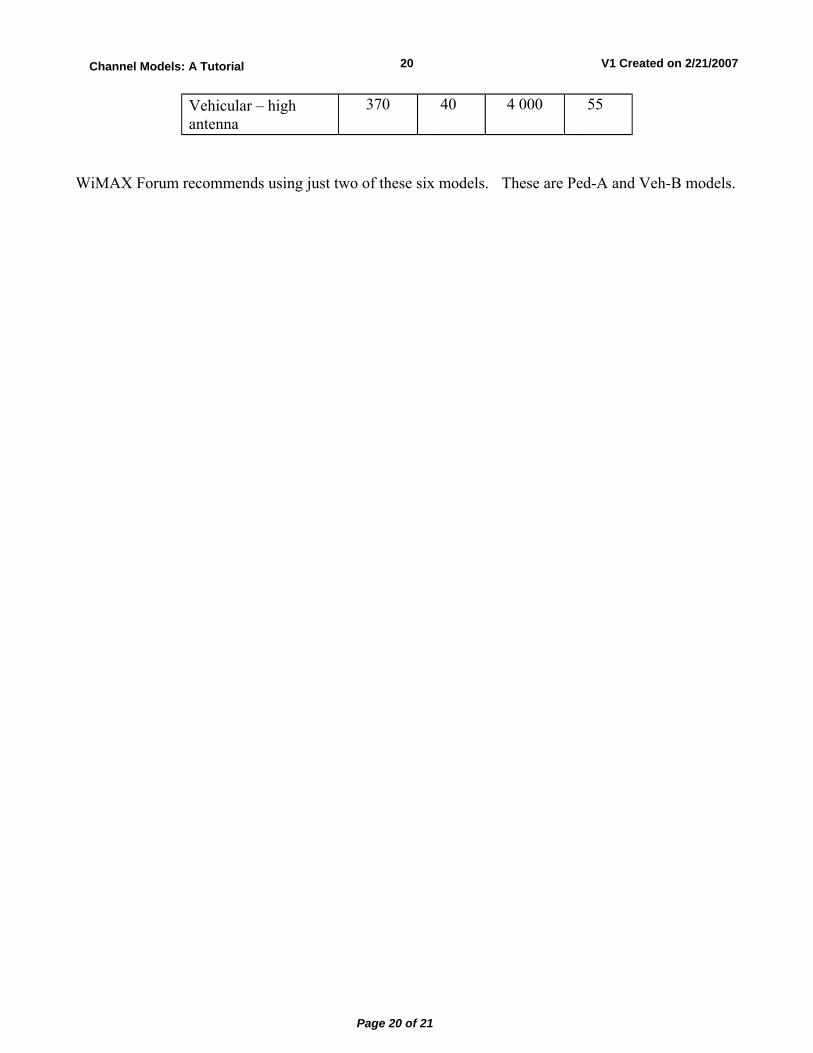
Page 20 of 21


Vehicular � high antenna

370 40 4 000 55

WiMAX Forum recommends using just two of these six models. These are Ped-A and Veh-B models.

Page 21 of 21


References [M.1225] ITU-R Recommendation M.1225, "Guidelines for evaluation of radio transmission technologies for IMT-2000," 1997

[Okumura1968] T. Okumura, E. Ohmore, and K. Fukuda, "Field strength and its variability in VHF and UHF land mobile service," Rev. Elec. Commun. Lab., pp. 825-73, September-October 1968.

[Hata1980] M. Hata, "Empirical formula for propagation kiss ub kabd nibuke radui services," IEEE Trans. Veh. Tech., pp. 317-25, August 1980.

[COST231] European Cooperative in the Field of Science and Technical Research EURO-COST 231, "Urban transmission loss models for mobile radio in the 900- and 1,800 MHz bands (Revision 2)," COST 231 TD(90)119 Rev. 2, The Hague, The Netherlands, September 1991, available at http://www.lx.it.pt/cost231/final_report.htm

[Ikegami1984] F. Ikegami, S. Yoshida, T. Takeuchi, and M. Umehira, �Propagation factors controlling mean field strength on urban streets,� IEEE Trans. on Antennas Propagation, vol. 32, no. 8, pp. 822�829, Aug. 1984.

[Walfisch1988] J. Walfisch, H. L. Bertoni, "A theoretical model of UHF propagation in urban environments," IEEE Trans. on Antennas and Propagation, vol. 36, no. 12, pp. 1788-1796, Dec. 1988

[Erceg1999] V. Erceg et. al, �An empirically based path loss model for wireless channels in suburban environments,� IEEE JSAC, vol. 17, no. 7, July 1999, pp. 1205-1211.

[Hari2000] K.V. S. Hari, K.P. Sheikh, and C. Bushue, �Interim channel models for G2 MMDS fixed wireless applications,� IEEE 802.16.3c-00/49r2, November 15, 2000, available as www.ieee802.org/16/tg3/contrib/802163c-00_49r2.pdf

[Erceg2001] V. Erceg, et al, "Channel Models for Fixed Wireless Applications," IEEE 802.16.3c-01/29r4, July 2001, available as www.ieee802.org/16/tg3/contrib/802163c-01_29r4.pdf

[Molisch2005] Andreas F. Molisch, "Wireless Communications," Wiley 2005, 622 pp. and associated web page http://www.wiley.com/legacy/wileychi/molisch/supp/appendices/Chapter_7_Appendices.pdf

[Goldsmith2005] Andrea Goldsmith, "Wireless Communications," Cambridge University Press, 2005, 644 pp.

[Andrews2007] Jeffrey G. Andrews, Arunabha Ghosh, and Rias Muhamed, "Fundamentals of WiMAX: Understanding Broadband Wireless Networking,", Prentice-Hall, February 2007, 496 pp.

[Cichon] Dieter J. Cichon, Thomas Kurner, "Propagation Prediction Models," Chapter 4, Available at www.it.lut.fi/kurssit/04-05/010651000/Luennot/Chapter4.pdf

Documents

Channel Models A Tutorialjain/cse574-08/ftp/channel_model... · Channel Models A Tutorial 1 V1.0 February 21, 2007 Please send comments/corrections/feedback to Raj Jain, [email protected]