Channel Modeling of Information ... - home.eps.hw.ac.uk

2 IEEE TRANSACTIONS ON VEHICULAR TECHNOLOGY, VOL. 60, NO. 1, JANUARY 2011

Channel Modeling of Information Transmission OverCognitive Interrogator-Sensor Networks

Yifan Chen, Member, IEEE, Wai Lok Woo, and Cheng-Xiang Wang, Senior Member, IEEE

Abstract—This paper looks into the modeling of informationtransmission over cognitive interrogator-sensor networks (CISNs),which represent a novel and important class of sensor networksdeployed for surveillance, tracking, and imaging applications. Thecrux of the problem is to develop a channel model that allowsfor the evaluation of the sensing channel capacity and error rateperformance in CISNs, for which the sensing link is overlaid bythe communication link. First, the layered discrete memorylesschannel and finite-state Markov channel models are identified asuseful tools to capture the essence of information transfer over thecommunication and sensing links in CISNs. Two different sensorencoding strategies, namely, 1) the amplify-modulate-and-forward(AMF) and 2) decode-modulate-and-forward (DMF) schemes, areconsidered. Subsequently, the concepts of double-directional chan-nel capacity azimuth spectrum (CCAS) and Chernoff informationazimuth spectrum (CIAS) are proposed to facilitate network-levelassessment of the communication and sensing link reliability. Astudy case considering a typical CISN for environmental moni-toring, conditioned on different wireless propagation and sensingconditions, is then presented to demonstrate the steps to derive thevarious model parameters. Finally, the potential applications ofthe proposed analytical framework in cognitive sensing, networkperformance assessment, and simulation are briefly discussed.

Index Terms—Channel capacity, Chernoff information, cog-nitive radar (CR), discrete memoryless channel (DMC), doubledirectional, finite-state Markov channel (FSMC), radio-frequencyidentification (RFID), wireless sensor network (WSN).

I. INTRODUCTION

COGNITIVE radar (CR) is an innovative concept for opti-mizing radar surveillance within a dynamic environment

[1]–[5]. A CR has the distinct capabilities of 1) being awareof its outside world by using previous measurements as well

Manuscript received February 25, 2010; revised July 15, 2010, August 28,2010, and October 13, 2010; accepted October 14, 2010. Date of publicationOctober 25, 2010; date of current version January 20, 2011. The work ofC.-X. Wang was supported in part by the Scottish Funding Council for theJoint Research Institute in Signal and Image Processing with the Universityof Edinburgh, as part of the Edinburgh Research Partnership in Engineeringand Mathematics (ERPem), and in part by RCUK for the U.K.–China ScienceBridges: R&D on (B)4G Wireless Mobile Communications. The review of thispaper was coordinated by Prof. C. P. Oestges.

Y. Chen is with the School of Electrical, Electronic and Computer Engi-neering, Newcastle University, NE1 7RU Newcastle upon Tyne, U.K., and alsowith the School of Computer, Electronics and Information, Guangxi University,Nanning 530004, China (e-mail: [email protected]).

W. L. Woo is with the School of Electrical, Electronic and ComputerEngineering, Newcastle University, NE1 7RU Newcastle upon Tyne, U.K.(e-mail: [email protected]).

C.-X. Wang is with the Joint Research Institute in Signal and Image Process-ing, School of Engineering and Physical Sciences, Heriot-Watt University,EH14 4AS Edinburgh, U.K. (e-mail: [email protected]).

Color versions of one or more of the figures in this paper are available onlineat http://ieeexplore.ieee.org.

Digital Object Identifier 10.1109/TVT.2010.2089545

as learning through interactions with the environment and2) intelligently and adaptively customizing the operation of itstransceivers in response to the channel variations in real time[1]. The feedback loop from the receiver to the transmitterfacilitates such a learning process.

There has also been a large amount of literature dealingwith wireless sensor networks (WSNs) over the past few yearsdue to their wide applications in environmental and habitatmonitoring, medical diagnostics, disaster management, struc-tural health monitoring, healthcare, etc. [6], [7]. In most of theexisting WSNs, a set of nodes measure data from a phenomenonof interest (POI) and then transmit them to a sink, where alldata are processed, and global decisions are made. Constrainedby limited energy resources and a lack of centralized coordi-nation, a cross-layer design that involves nonconvex nonlinearoptimization should be applied to optimize energy consumptionin communication and computation [8], and multihop wirelessconnectivity is usually employed to forward data to and fromthe sink [9].

Radio-frequency identification (RFID) technology is com-monly used to store and retrieve data through RF transmission[9]. An RFID system consists of readers (or interrogators) andtags (or transponders). A tag has a unique identification numberand memory that stores additional data. In a typical RFID ap-plication, readers communicate with tags in their wireless rangeand collect information about the objects to which tags areattached, such as manufacturer name, product type, and envi-ronmental factors, including temperature, humidity, and so on.

In this paper, we develop a novel network architecturethat combines CR, WSN, and RFID and call it a cogni-tive interrogator-sensor network (CISN) [10]. As illustratedin Fig. 1, the CISN constitutes a dynamic closed feedbackloop encompassing the interrogator, environment, and sink.Here, the environment comprises the communication chan-nel (interrogator → sensor → sink) and the sensing channel(POI → sensor). The whole system works as follows.

1) The interrogator sends input signals to activate all sensorsin the WSN, which in turn monitor the surroundings todetect a POI.

2) Based on readings collected at sensors, the input datafrom the interrogator are modulated accordingly andrelayed to the sink for central processing and decisionmaking.

3) The interrogator and the sink form a CR system,which continuously learns about the environment throughknowledge gained from interactions with the environmentand updates the sink with relevant information on theenvironment.

0018-9545/$26.00 © 2010 IEEE

CHEN et al.: CHANNEL MODELING OF INFORMATION TRANSMISSION OVER CISNS 3

Fig. 1. CISN combining CR, WSN, and RFID technologies.

4) The interrogator adjusts its transmitted signals in a robustand effective manner by taking into account the feedbackfrom the sink. The probing signals may also commandthe sensors to make adjustments to their sensing andencoding processes.

A CISN conserves power and bandwidth because the networkattempts to minimize energy usage by turning off sensor nodeswhen no communication needs to occur.

A. Related Works

One fundamental building block of the CISN architecture isa network of sensors with the capability to 1) monitor physicalor environmental conditions, 2) store and process information,3) modulate and demodulate an external “wake-up” signal, and4) receive and transmit the signal. The first two properties areassociated with the traditional WSNs, whereas the last twoare related to the RFID, particularly in terms of modulating/demodulating the wake-up signal. Consequently, these proper-ties require integration of WSN and RFID technologies, whichhas become feasible in recent years thanks to technologicalimprovements in the miniaturization of sensors, energy savings,and the integration of multiple sensing device within a singlenode [9], [11]–[23]. In [9], four types of application scenariosfor combining RFID and WSNs were discussed: 1) integratingRFID tags with sensors [11]–[19]; 2) integrating tags with WSNnodes and wireless devices [20]; 3) integrating RFID readerswith WSN nodes and wireless devices [21]; and 4) a mix ofRFID components and WSNs [22], [23].

The CISN is well suited for the first and most investigatedtype of integration [11]–[19]. The overall functionalities andcapacities of the interrogator and the sink in Fig. 1 (except forthe feedback loop) are similar to those of an ambient high-power RFID reader, which scans multiple sensor tags in theWSN concurrently and collects information from the network.The sensors in Fig. 1 are essentially RFID tags, which mayuse the RFID protocols and mechanisms to send tag identifiersas well as to share sensed data. Due to the advance in low-power electronics, it is now feasible to envisage a low-costultralow-power integrated RFID tag that provides power-harvesting, sensing, and actuating capabilities [11]–[13], [15]–[19]. Such an RFID-tag-and-sensor integration framework may

find important applications in bio-monitoring of patients andthe elderly [11], [13], [15], [16], cyber-centric monitoring [17],and prognostics and health management [19].

Another important operating block of the CISN is a fullyadaptive transmission and reception system with the capa-bility to observe and learn from the environment and adaptits transmission characteristics accordingly. These cognitivesensing features require a feedback loop from the sink tothe interrogator [1]–[4], [24], [25], which could be achievedthrough integration of the CR and RFID reader. The interroga-tor and the sink can be collocated (i.e., a monostatic radarconfiguration) and correspond to the transmission and receptionmodules housed in the same RFID reader circuit. Otherwise,they can be separated by a distance with a feedback connection(i.e., a bistatic arrangement). Nevertheless, little work has beenreported in the open literature concerning such integration. Notethat incorporating CR into the RFID reader would naturally leadto the integration of CR and WSN through RFID sensor tags.

In brief, the proposed CISN calls for the seamless integrationof CR, WSN, and RFID technologies, for which partial integra-tion has already been achieved. To the best of our knowledge, sofar, the channel modeling of information transmission over suchnetworks has not explicitly been taken into account to assist indesigning an integration architecture. The main objective of thecurrent paper is thus to fill this research gap.

B. Main Contributions of This Paper

There is a fundamental difference between CISNs andtraditional communication networks in terms of informationprocessing. In the former case, we are interested in the dif-ferential information between the inputs and outputs of theCR system, which would be correlated with the POI undersurveillance. On the other hand, in the latter case, the differencebetween the inputs and outputs should be zeroed to achieveideal information delivery. Therefore, it is very important todevelop a new theoretical model for the representation andanalysis of CISNs. The main contributions of this paper aresummarized as follows.

1) We consider two types of information-transmissionmodels: 1) discrete memoryless channel (DMC) and2) finite-state Markov channel (FSMC) [26]–[28], whichare applicable to static and dynamic noisy processes,respectively. Subsequently, the layered DMC and FSMCmodels are proposed to describe the input–output rela-tionship in a CISN.

2) We introduce two novel sensor encoding strategiesfor CISN: 1) amplify-modulate-and-forward (AMF) and2) decode-modulate-and-forward (DMF), which are par-allel to the amplify-and-forward and decode-and-forwardtechniques in cooperative diversity [29]–[32], with theonly difference being that an intermediate “modulate”step is included.

3) We develop the double-directional channel capacity az-imuth spectrum (CCAS) and the Chernoff informationazimuth spectrum (CIAS) to describe the network-scalelink quality.


This paper is organized as follows: In Section II, we establishthe general channel modeling methodology for CISNs. Fur-thermore, a canonical cognitive sensing problem is formulatedbased on the proposed models. In Section III, a typical CISN forenvironmental monitoring is presented as a study case, wherekey model parameters are identified subject to various wirelesscommunication and sensing scenarios. Numerical examples areprovided in Section IV based on the discussions in Section III.Section V sheds some light on the potential applications of theproposed methodology. Finally, some concluding remarks aredrawn in Section VI.

II. COGNITIVE INTERROGATOR-SENSOR NETWORK

CHANNEL MODELING METHODOLOGY

A. General Principles

A CISN involves information transmission over two links:1) the communication link “interrogator → sensor → sink” and2) the sensing link “POI → sensor,” as shown in Fig. 1. Toallow for a binary-input–binary-output formulation of these tworandom processes, we may assume that the sensor is able to en-code the continuous-valued POI information into a sequence ofbinary digits, as demonstrated in the following three examples.

1) Body Sensor Network: There has been a growing inter-est in the field of body sensor networks for pervasivehealthcare applications [13], [33]. Commonly, sensors areplaced on the human body to measure specified vital-signdata. These body-worn sensors are simultaneously con-nected to the gateway that coordinates individual nodesthrough wireless connectivity. The sensed data may in-clude physiological signals such as electrocardiogram orelectroencephalogram. Each sensor can perform standardscalar quantization that maps analog real vital-sign valuesinto discrete real values, which can then be mapped intobinary strings using a code book [34].

2) Binary Sensor Network: In the decentralized detectionproblem, a set of dispersed binary sensor nodes collectinformation about the POI. Each node receives an analogobservation waveform, which is sampled and expressedas a sequence of observations. At each discrete time, thesensor is required to make a binary decision about the POIbased on an admissible strategy. The sensor will output 0if the POI is believed to be absent and output 1 otherwise[35]. Hence, the sensor converts the sensed data into abinary sequence, indicating the presence or absence ofthe POI.

3) Radar Target Detection: Consider the classical radar de-tection problem, which assumes a far-field point sourcetarget when the radar pulse is narrowband so that therange span of the target is well within a single range cell[36]. Assume that a radar is scanning the surveillancedomain to detect a dominant reflecting target. In digitalform, the transmitter sends a binary probing sequence(x1, . . . , xK), and the receiver observes an output se-quence feedback from the environment (y1, . . . , yK). Forany range cell under surveillance, if an ideal “lossless”reflector is present, then it will either relay the same

input data to the receiver (i.e., without phase inversion)or flip all the input bits and then forward them to thereceiver (i.e., with phase inversion), depending on itsdielectric properties, as compared with the surroundingmedium [37]. Effectively, the operation can be expressedas yk = xk ⊕ ak ⊕ ηk (k = 1, 2, . . . ,K), where ak = 0or ak = 1 corresponds to the situation without or withphase inversion, respectively. The term ηk is the binarychannel noise bit, and ⊕ is the module-2 addition. On theother hand, in the absence of a reflector at the range cellunder observation, the output yk is dominated by noise,which is given as yk = ηk. Hence, we could interpretthe radar target as a virtual sensor, which transforms theinformation about its location into either an all-one or all-zero sequence.

Following from the foregoing discussions, the CISN canbe represented using two binary-input–binary-output equationsdescribed by

yk =xk ⊕ bk ⊕ ηk (1)bk = ak ⊕ θk. (2)

Here, xk and yk are the communication link input (data trans-mitted from the interrogator) and output (data received at thesink), respectively; ak and bk are the sensing link input (idealPOI data without noise corruption) and output (actual POI dataused to modulate the probing signals from the interrogator),respectively; ηk and θk are the communication and sensingnoise, respectively; and k is the discrete time index. Further-more, xk, yk, ak, bk, ηk, θk ∈ {0, 1}, and ηk and θk are twostatistically independent processes. These two equations implythat the sensor will behave like a typical relay when bk = 0,which upon reception of the interrogating signal will forwardthe same message to the receiver. On the other hand, whenbk = 1, the input data bit will be inverted and then retransmittedto the receiver.

We can broadly categorize the sensor functionality as ei-ther nonregenerative or regenerative. In the former case, thesensor amplifies, modulates, and forwards the received signal,whereas in the latter case, the sensor decodes, modulates, andforwards the received signal. These two schemes are parallel tothe amplify-and-forward and decode-and-forward techniques incooperative diversity [29]–[32], with the only difference that anintermediate “modulate” step is included in AMF and DMF toallow the relayed signal to carry information about the POI.Equations (1) and (2) are well suited for an AMF scheme, butfor a DMF system, ηk in (1) should further be decoupled into

ηk = ηB,k ⊕ ηF,k. (3)

In the preceding equation, ηB,k and ηF,k are associated withthe noise processes of the backward channel (interrogator →sensor) and the forward channel (sensor → sink), respectively.Nevertheless, we may establish an equivalent AMF channelfrom the underlying DMF channel by applying the followingtheorem on cascading two independent binary symmetric chan-nels (BSCs).

Theorem 1—Cascading of Two BSCs: If ηB,k and ηF,k

can be described by two independent BSCs with raw error


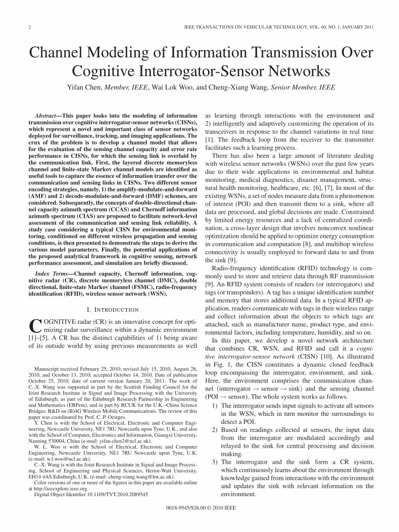
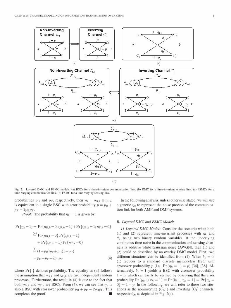
Fig. 2. Layered DMC and FSMC models. (a) BSCs for a time-invariant communication link. (b) DMC for a time-invariant sensing link. (c) FSMCs for atime-varying communication link. (d) FSMC for a time-varying sensing link.

probabilities pB and pF, respectively, then ηk = ηB,k ⊕ ηF,k

is equivalent to a single BSC with error probability p = pB +pF − 2pBpF.

Proof: The probability that ηk = 1 is given by

Pr{ηk =1}= Pr{ηB,k =0; ηF,k =1}+Pr{ηB,k =1; ηF,k =0}(a)= Pr{ηB,k =0}Pr{ηF,k =1}

+ Pr{ηB,k =1}Pr{ηF,k =0}(b)= (1−pB)pF+pB(1−pF)

= pB+pF−2pBpF (4)

where Pr{·} denotes probability. The equality in (a) followsthe assumption that ηB,k and ηF,k are two independent randomprocesses. Furthermore, the result in (b) is due to the fact thatboth ηB,k and ηF,k are BSCs. From (4), we can see that ηk isalso a BSC with crossover probability pB + pF − 2pBpF. Thiscompletes the proof. �

In the following analysis, unless otherwise stated, we will usea generic ηk to represent the noise process of the communica-tion link for both AMF and DMF systems.

B. Layered DMC and FSMC Models

1) Layered DMC Model: Consider the scenario when both(1) and (2) represent time-invariant processes with ηk andθk being two binary random variables. If the underlyingcontinuous-time noise in the communication and sensing chan-nels is additive white Gaussian noise (AWGN), then (1) and(2) could be described by an overlay DMC model. First, twodifferent situations can be identified from (1). When bk = 0,(1) reduces to a standard discrete memoryless BSC withcrossover probability p (i.e., Pr{ηk = 1} = p) [34], [38]. Al-ternatively, bk = 1 yields a BSC with crossover probability1 − p, which can easily be verified by observing that the errorprobability Pr{yk ⊕ xk = 1} ≡ Pr{bk ⊕ ηk = 1} = Pr{ηk =0} = 1 − p. In the following, we will refer to these two situ-ations as the noninverting (CNI) and inverting (CI) channels,respectively, as depicted in Fig. 2(a).


Subsequently, the underlying law that governs the transitionbetween CNI and CI is given by (2), which could be modeledusing a DMC with two different error probabilities qNI and qI,as shown in Fig. 2(b) (i.e., Pr{θk = 1} = qNI if ak = 0 andPr{θk = 1} = qI if ak = 1). The main reason to use an input-dependent DMC instead of a BSC is due to the specific featuresassociated with a sensing link, which will be made clear inSection III-A.

In brief, a layered DMC model comprising the DMC inFig. 2(b) overlaid by the two BSCs in Fig. 2(a) can be employedto characterize the input–output relationship in a CISN if boththe wireless propagation channel and the POI are time invariant.

2) Layered DMC/FSMC Model: If (1) is a time-varyingprocess and (2) is time invariant, then we can still apply theDMC in Fig. 2(b) to model (2). However, two FSMCs, asshown in Fig. 2(c), should be used to characterize the time-varying fading channel in (1). When bk = 0, we can define astandard FSMC for the noninverting channel CNI [26], [39].Each state is associated with a BSC. For example, the crossoverprobabilities for the two states of CNI in Fig. 2(c), i.e., S0 andS1, are p0 (i.e., Pr{ηk = 1} = p0) and p1 (i.e., Pr{ηk = 1} =p1), respectively. The analytical expressions for states, statetransition probabilities, and error probabilities in each stateconditioned on the time-varying communication link processfollow the widely used techniques in [27]. On the other hand,bk = 1 results in a similarly structured FSMC with “inverting”states S̄0 and S̄1, where the crossover probabilities are given by1 − p0 and 1 − p1, respectively. This phenomenon can readilybe proved following the same approach in Section II-B1. Thistype of Markov chain gives rise to the inverting channel CI.Hence, a layered FSMC-DMC model that comprises the DMCin Fig. 2(b) overlaid by the two FSMCs in Fig. 2(c) should beemployed to describe the input–output relationship in a CISN.

Conversely, if (1) is time invariant but (2) is time varying,we can make use of the two BSCs in Fig. 2(a) to describe(1). However, an FSMC, as illustrated in Fig. 2(d), should beconsidered for the time-varying process in (2) [39]. Each statein Fig. 2(d) is associated with a DMC. For example, the errorprobabilities for state S0 in Fig. 2(d) are given as qNI,0 (i.e.,Pr{θk = 1} = qNI,0 if ak = 0) and qI,0 (i.e., Pr{θk = 1} =qI,0 if ak = 1). Moreover, all the other model parameters canbe derived following the approach similar to that in [27]. Insummary, a layered DMC-FSMC model that comprises theFSMC in Fig. 2(d) overlaid by the two BSCs in Fig. 2(a) shouldbe used to explain the input–output relationship in a CISN inthis situation.

3) Layered FSMC Model: Finally, the most complex sce-nario occurs when both (1) and (2) are time-varying processes.In such a case, a layered FSMC model that consists of theMarkov chain in Fig. 2(d) overlaid by the Markov chains inFig. 2(c) is appropriate for synthesizing the two input–outputequations in (1) and (2), respectively.

C. Double-Directional CCAS and CIAS

Analogous to the fact that the signal power is flowing througha physical multipath channel, the relevant substance that isflowing through a virtual CISN is the information delivered

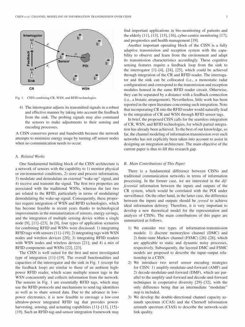
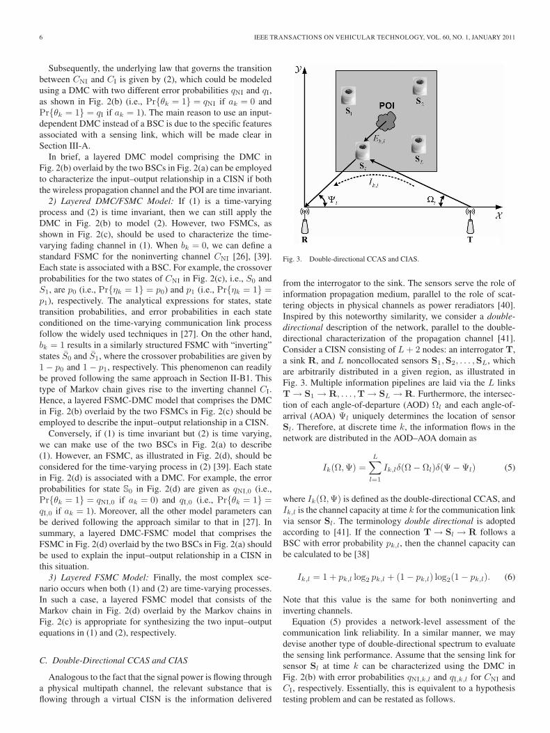
Fig. 3. Double-directional CCAS and CIAS.

from the interrogator to the sink. The sensors serve the role ofinformation propagation medium, parallel to the role of scat-tering objects in physical channels as power reradiators [40].Inspired by this noteworthy similarity, we consider a double-directional description of the network, parallel to the double-directional characterization of the propagation channel [41].Consider a CISN consisting of L + 2 nodes: an interrogator T,a sink R, and L noncollocated sensors S1,S2, . . . ,SL, whichare arbitrarily distributed in a given region, as illustrated inFig. 3. Multiple information pipelines are laid via the L linksT → S1 → R, . . . ,T → SL → R. Furthermore, the intersec-tion of each angle-of-departure (AOD) Ωl and each angle-of-arrival (AOA) Ψl uniquely determines the location of sensorSl. Therefore, at discrete time k, the information flows in thenetwork are distributed in the AOD–AOA domain as

Ik(Ω,Ψ) =L∑

l=1

Ik,lδ(Ω − Ωl)δ(Ψ − Ψl) (5)

where Ik(Ω,Ψ) is defined as the double-directional CCAS, andIk,l is the channel capacity at time k for the communication linkvia sensor Sl. The terminology double directional is adoptedaccording to [41]. If the connection T → Sl → R follows aBSC with error probability pk,l, then the channel capacity canbe calculated to be [38]

Ik,l = 1 + pk,l log2 pk,l + (1 − pk,l) log2(1 − pk,l). (6)

Note that this value is the same for both noninverting andinverting channels.

Equation (5) provides a network-level assessment of thecommunication link reliability. In a similar manner, we maydevise another type of double-directional spectrum to evaluatethe sensing link performance. Assume that the sensing link forsensor Sl at time k can be characterized using the DMC inFig. 2(b) with error probabilities qNI,k,l and qI,k,l for CNI andCI, respectively. Essentially, this is equivalent to a hypothesistesting problem and can be restated as follows.


Problem 1: At time k, sensor Sl decides between two alter-native hypotheses H0 (“Channel is CNI”) and H1 (“Channel isCI”) subject to the probability of detection Pr{bk,l = 1|H1} =1 − qI,k,l and the probability of false alarm Pr{bk,l = 1|H0} =qNI,k,l, where bk,l is the output of the sensing link [cf. (2)]. Thebest achievable error exponent for this problem is given by theChernoff information [38] as

Ek,l=− min0≤ε≤1

log2

⎧⎨⎩

∑bk,l∈{0,1}

[Pr{bk,l|H0}]ε[Pr{bk,l|H1}]1−ε

⎫⎬⎭

=− min0≤ε≤1

log2

{[Pr{0|H0}]ε[Pr{0|H1}]1−ε

+ [Pr{1|H0}]ε[Pr{1|H1}]1−ε}

=− min0≤ε≤1

log2

[(1−qNI,k,l)εq1−ε

I,k,l+qεNI,k,l(1−qI,k,l)1−ε

].

(7)

For simplicity, we will consider the Bhattacharyya distancein this paper, which is a special case of Chernoff informa-tion [38], as given by Ek,l = − log2[(1 − qNI,k,l)1/2q

1/2I,k,l +

q1/2NI,k,l(1 − qI,k,l)1/2].

Subsequently, we can define the double-direction CIAS as

Ek(Ω,Ψ) =L∑

l=1

Ek,lδ(Ω − Ωl)δ(Ψ − Ψl) (8)

which offers a network-scale evaluation of the sensing linkquality.

D. Canonical Cognitive Sensing Problem

Let us consider time-varying communication and sensingchannels. We will use the superscript k̂ to indicate the slowtime index for symbol vectors or system-level parameters (e.g.,system operational modes or performance measures) at eachround of global adaptation. This should be distinguished fromthe subscript k that represents the fast time index for elementscollected in symbol vectors. Furthermore, the subscripts T, S,and R will be used to denote the quantities associated withthe interrogator, sensor, and sink, respectively. Subsequently,the following variables at discrete time k̂ for a CISN can bedefined:

1) Bk̂T: beamforming strategy at the interrogator;

2) Bk̂R: beamforming strategy at the sink;

3) X k̂ Δ= (xk̂1 , xk̂

2 , . . . , xk̂K): input binary sequence transmit-

ted from the interrogator, where K is the length of thesequence at time k̂;

4) Y k̂ Δ= (yk̂1 , yk̂

2 , . . . , yk̂K): output binary sequence received

at the sink;5) Ck̂ Δ= {Ck̂

1 , Ck̂2 , . . . , Ck̂

L}: coding strategies of sensors (i.e.,mapping of continuous-valued sensing data into bi-nary sequences) administered by the interrogator, whereCk̂

l (l = 1, 2, . . . , L): the admissible strategy at sensor Sl;

6) Lk̂ Δ= {lk̂1 , lk̂2 , . . . , lk̂L}: location estimate of sensors at thesink, where lk̂l (l = 1, 2, . . . , L) denotes the location esti-mate of sensor Sl;

7) Pk̂ Δ= {pk̂1 ,pk̂

2 , . . . ,pk̂L}: estimated layered FSMC model

parameters [cf. Fig. 2(c) and (d)] for all the sensors, wherepk̂

l (l = 1, 2, . . . , L) denotes the estimated parameter setfor sensor Sl.

Subsequently, a canonical cognitive sensing problem can beformulated as follows.

Problem 2:

Given Bk̂T,Bk̂

R,X k̂, Y k̂, Ck̂,Lk̂,Pk̂

Optimize Mk̂+1 at time k̂+1

Subject to Bk̂+1T ∈BT,Bk̂+1

R ∈BR,X k̂+1∈X, Ck̂+1∈C.

The optimization criteria Mk̂+1 represents a specific systemperformance measure under consideration, which may be thecommunication channel capacity, sensing error rate, sensingwaveform fidelity, etc. BT, BR, X, and C are the admissiblesets of relevant strategies or system parameters. Note that theforegoing canonical problem can easily be applied to othertypes of communication or sensing channels.

III. DERIVATION OF MODEL PARAMETERS IN A TYPICAL

COGNITIVE INTERROGATOR-SENSOR NETWORK

A. Time-Invariant Wireless Channel and POI

When both the wireless channel and the POI are time invari-ant, the information transfer over a CISN can be characterizedby using the layered DMC model presented in Section II-B1.

The simplest case of a time-invariant communication link isan AWGN channel [42]. It is assumed that the average powertransmitted by the interrogator and the sensor is Pt

T and PtS,

respectively, where the superscript t denotes the transmittedsignal. For simplicity, we further assume that both the sensorand sink receiver chains have identical noise properties andhence the same AWGN power. Nevertheless, the followinganalysis is also applicable to systems with unequal sensor andsink noise power.

1) AMF System: For an AMF system, the wireless channelconsists of two portions: the 1) backward (interrogator → sen-sor) and 2) forward (sensor → sink) links, as depicted in Fig. 1.The following received signal at the sink yR(t) comprises threecomponents, as demonstrated in [30]:

yR(t) = hFhBxS(t) + hFn(t) + n(t) (9)

where n(t) is the AWGN waveform, and xS(t) is the unit-variance modulated signal sent by the sensor. The two variableshB and hF correspond to the backward and forward channels,respectively, which can be calculated as [5]

hB =√

PtTAd

−κ2

1 and hF =√

GSAd−κ

22 . (10)

In (10), A is a constant, GS is the power amplification factorof the sensor, and κ is the path loss exponent. d1 and d2


are the propagation distances for the backward and forwardconnections, respectively, as shown in Fig. 1. For simplicity, wewill consider a fixed gain sensor (parallel to a fixed gain relayin cooperative diversity systems [30], [31]) with

GS =Pt

S

E {PrS}

=Pt

S

PtTA2d−κ

1 + σ2n

. (11)

E{·} is the statistical expectation operation, and PrS is the

power received at the sensor, where the superscript r denotes thereceived signal. σ2

n is the power of the AWGN in the backwardlink. Substituting (10) and (11) into (9) yields

yR(t) =hFhBxS(t) + (hF + 1) n(t)

=

√Pt

S

1 + σ2n/

(PtTA2d−κ

1

)Ad−κ

22 xS(t)

+

(√Pt

S

PtTA2d−κ

1 + σ2n

Ad−κ

22 + 1

)n(t) (12)

where the first term is the desired signal, whereas the secondterm is the overall AWGN.

Subsequently, CNI and CI are defined by the BSCs inFig. 2(a). For binary phase-shift keying (BPSK), the crossoverprobability for CNI is given by [42]

p=Q⎛⎝√

2(

hFhB

hF+1

)2

γ

⎞⎠

=Q

⎛⎜⎜⎜⎜⎝√√√√√√

2PtSA2d−κ

2 γ[1+ σ2

n

PtT

A2d−κ1

] [√ PtS

A2d−κ2 /σ2

n

PtT

A2d−κ1 /σ2

n+1+1

]2

⎞⎟⎟⎟⎟⎠ . (13)

The Q(·) function is the complementary cumulative normaldistribution. γ = Eb/N0, where Eb is the average energy per bitfor the unit-variance signal xS(t), and N0 is the noise spectraldensity of n(t).

2) DMF System: For a DMF system, the signal received atthe sensor is written as

yS(t) = hBxT(t) + n(t) (14)

where xT(t) is the unit-variance waveform sent by the inter-rogator with the same average energy per bit as that of xS(t),and hB is given in (10). For BPSK, the backward channel canbe described by a BSC with error probability

pB = Q(√

2h2Bγ

)= Q

(√2Pt

TA2d−κ1 γ

). (15)

Furthermore, the signal received at the sink from the sensor(after decoding and modulating) is

yR(t) = h′FxS(t) + n(t) (16)

where h′F =

√PtSAd

−(κ/2)2 . For BPSK, the forward channel

can be described by a BSC with crossover probability as

pF = Q(√

2 (h′F)2 γ

)= Q

(√2Pt

SA2d−κ2 γ

). (17)

Substituting (15) and (17) into (4) gives the error probability ofthe equivalent single BSC for the DMF system.

3) POI: The simplest model for the POI is a time-invariantisotropic signal source with path loss factor β [43], whichdepends on the type of signal considered (chemical contami-nation, sound, radioactive radiation, etc.). Thus, the receivedsignal strength at the sensor ρk after appropriate sampling andprocessing is

ρk ={

wk, when POI is absentρ0D

−β + wk, when POI is present(18)

where k = 1, 2, . . .; ρ0 is the signal strength measured at 1 mfrom the POI location; D is the distance between the POI andthe sensor, as shown in Fig. 1; and wk is the AWGN corruptingthe observation. Let us consider binary quantization, where thesensor will flip the bit received from the interrogator if and onlyif ρk is larger than a sensing threshold ρ∗. As a result, the errorprobability for CNI in Fig. 2(b) is given by

qNI = Pr{wk > ρ∗|CNI} = Q(

ρ∗

σw

)(19)

where σw is the standard deviation of the noise. On the otherhand, the error probability for CI in Fig. 2(b) is

qI =Pr{ρ0D−β+wk≤ρ∗|CI}=1−Q

(ρ∗−ρ0D

−β

σw

). (20)

Note that qNI = qI if and only if ρ∗ = ρ0D−β/2. In this case,

the DMC in Fig. 2(b) would reduce to a standard BSC.

B. Time-Varying Wireless Channel and Time-Invariant POI

When the wireless channel is time varying and the POI istime invariant, the information transfer over a CISN can bedescribed through the layered FSMC-DMC model presented inSection II-B2.

1) AMF System: We will first consider an AMF scheme. Ifthe nonstationarity of the propagation environment is caused bythe motion of sensors (e.g., sensing devices mounted on movingvehicles), narrowband fading will occur, which is describedas [30]

yR(t)=hFhBh̃F(t)h̃B(t)xS(t)+hFh̃F(t)n(t)+n(t) (21)

where hB and hF are given in (10). h̃B(t) and h̃F(t) are theunit-variance complex fading coefficients for the backward andforward channels, respectively. In general, it is difficult to ob-tain a closed-form statistical analysis of the instantaneous SNRfor (21) [30]. Nevertheless, the problem can be simplified when|hFh̃F(t)|2 1, which is satisfied if Pt

S PtT following (10)

and (11). This condition is common because the sensors areusually power constrained, whereas the interrogator, like theRFID reader, is of high transmit power [11]–[19]. In this case,


the noise term hFh̃F(t)n(t) would be much less than n(t) and,hence, can be neglected.

If the fading envelopes for both up and down links exhibitan identical and independent Rayleigh distribution, the overallenvelope α = |h̃B||h̃F| is double-Rayleigh faded [30], i.e.,

fα(α) = 4αK0(2α). (22)

The K0(·) function is the zeroth-order Bessel function of thesecond kind. We assume isotropic antennas operating in a 2-Disotropic scattering environment [30]. The level crossing rate(LCR) of α at level α∗, which is defined as the rate at which thechannel envelope crosses α∗, is [30]

Lα(α∗) =4√

πα∗√

2

∞∫0

1z2

exp[− (α∗)2 + z4

z2

]

×√

ν2z4 + ν2(α∗)2dz (23)

where ν is the maximum Doppler shift induced by the motionof the sensor.

Next, we construct the simplest two-state FSMC [or theGilbert–Elliott channel (GEC)], as illustrated in Fig. 2(c),where each state corresponds to a specific channel qualityclassified according to a threshold level α∗ [27]. That is, thedouble-Rayleigh fading channel is said to be in state S0 (or the“bad” state in the GEC) and state S1 (or the “good” state inthe GEC) if the fading envelope is in the intervals [0, α∗) and[α∗,∞], respectively. Following the methodology in [27], thesteady-state probability of each state is

Π0 =

α∗∫0

fα(α)dα =

α∗∫0

4αK0(2α)dα (24)

Π1 = 1 − Π0 = 1 −α∗∫0

4αK0(2α)dα. (25)

The state transition probabilities are related to the LCRs and thesteady-state probabilities through the following relationships[27]:

P0→1 =Lα(α∗)Ts

Π0(26)

P1→0 =Lα(α∗)Ts

Π1(27)

where Ts is the symbol period. Other state transition proba-bilities are given as P0→0 = 1 − P0→1 and P1→1 = 1 − P1→0.Finally, the average crossover probability for each state is [27]

p0 =

∫ α∗

0 p(α)fα(α)dα

Π0

=

∫ α∗

0 Q(√

2PtS

A2α2d−κ2 γ

1+σ2n/(Pt

TA2d−κ

1 )

)4αK0(2α)dα∫ α∗

0 4αK0(2α)dα(28)

p1 =

∫∞α∗ p(α)fα(α)dα

Π1

=

∫∞α∗ Q

(√2Pt

SA2α2d−κ

2 γ

1+σ2n/(Pt

TA2d−κ

1 )

)4αK0(2α)dα

1 − ∫ α∗0 4αK0(2α)dα

(29)

where p(α) is the crossover probability for a specific fadingcoefficient α and is derived following (13) and assuming Pt

S Pt

T. The foregoing analysis can easily be extended to moregeneral FSMCs with more than two states.

2) DMF System: When a DMF scheme is adopted, thefading signal received at the sensor is

yS(t) = hBh̃B(t)xT(t) + n(t). (30)

Following Section III-B1, the fading envelope αB = |h̃B| isRayleigh distributed with unit variance per complex dimensiongiven as

fαB(αB) = 2αB exp(−α2

B

). (31)

The LCR at an amplitude boundary threshold α∗B is [42]

LαB (α∗B) =

√2πα∗

Bν exp[− (α∗

B)2]

(32)

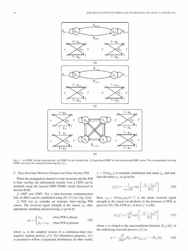
with ν being the maximum Doppler frequency shift.For this backward connection, we can easily establish the

GEC, as shown in Fig. 4(a), following the practice in [27]. Thechannel is said to be in state SB,0 and state SB,1 if the fadingenvelope is in the intervals [0, α∗

B) and [α∗B,∞], respectively.

The steady-state probabilities are obtained as

ΠB,0 =

α∗B∫

0

fαB(αB)dαB = 1 − exp[− (α∗

B)2]

(33)

ΠB,1 = 1 − ΠB,0 = exp[− (α∗

B)2]. (34)

Finally, the state transition probabilities PB,i→j (i, j ∈ {0, 1})and the average crossover probabilities pB,i (i ∈ {0, 1}) canbe calculated following (26)–(29) by substituting the relevantparameters for the backward channel. In a similar manner, wecan construct the GEC for the sensor-to-sink connection asdepicted in Fig. 4(b), where the subscript F is used to replacethe subscript B to indicate the forward channel.

The cascading of two GECs is equivalent to a four-stateFSMC, as illustrated in Fig. 4(c), where each state is de-

fined as SijΔ= {SB = SB,i, SF = SF,j} (i, j ∈ {0, 1}). As-

suming independence between the backward and forwardchannels, the steady-state probabilities are Πij = ΠB,i ×ΠF,j , and the state transition probabilities are Pi1j1→i2j2 =PB,i1→i2 × PF,j1→j2 (i1, j1, i2, j2 ∈ {0, 1}). By applying (4),the crossover probabilities are calculated to be pij = pB,i +pF,j − 2pB,ipF,j .

3) POI: For a time-invariant POI, the formulations in(18)–(20) can readily be applied to determine its DMC modelparameters, which govern the transition between CNI and CI

[cf. Fig. 2(b)].


Fig. 4. (a) FSMC for the backward link. (b) FSMC for the forward link. (c) Equivalent FSMC for the noninverting DMF system. The corresponding invertingFSMC can easily be constructed following Fig. 2(c).

C. Time-Invariant Wireless Channel and Time-Varying POI

When the propagation channel is time invariant and the POIis time varying, the information transfer over a CISN can bemodeled using the layered DMC-FSMC model discussed inSection II-B2.

1) AMF and DMF: For a time-invariant communicationlink, its BSCs can be established using (9)–(17) [cf. Fig. 2(a)].

2) POI: Let us consider an isotropic time-varying POIsource. The received signal strength at the sensor ρk, afterappropriate sampling and processing, is given by

ρk =

{wk, when POI is absent

ρ̂k + wk, when POI is present(35)

where ρ̂k is the sampled version of a continuous-time non-negative random process ρ̂(t). For illustration purposes, ρ̂(t)is assumed to follow a lognormal distribution. In other words,

ζ = 10 log10 ρ̂ is normally distributed with mean ζm and stan-dard deviation σζ , as given by

fζ(ζ) =1

σζ

√2π

exp

[− (ζ − ζm)2

2σ2ζ

]. (36)

Here, ζm = 10 log10(ρ0D−β) is the mean received signal

strength at the sensor (in decibels) in the presence of POI, asgiven in (18). The LCR of ζ at level ζ∗ is [44]

Lζ(ζ∗) =√

�

2πexp

[− (ζ∗ − ζm)2

2σ2ζ

](37)

where � is related to the autocorrelation function Rζζ(Δt) ofthe underlying Gaussian process ζ(t) as

� = − d2

dΔt2Rζζ (Δt)|Δt=0 = −R̈ζζ(0). (38)


If the temporal correlation properties of ζ(t) follow a Gaussianmodel [44]

Rζζ(Δt) = exp

[−(

Δt

τD

)2]

(39)

with τD being the decorrelation time, it follows that the quan-tity � = −R̈ζζ(0) = 2/τ2

D, and Lζ(ζ∗) can easily be analyzedusing (37).

The next step is to construct a two-state FSMC model tocharacterize the transition between CNI and CI, as illustratedin Fig. 2(d). By applying the same approach used to define anFSMC in fading channels, as discussed in Section III-B, thesensing link is said to be in state S0 and state S1 if the receivedPOI strength ζ is in the intervals (−∞, ζ∗) and [ζ∗,∞), respec-tively. The steady-state probability of each state is derived byintegrating the distribution function of the received POI overthe corresponding region, where

π0 =

ζ∗∫−∞

fζ(ζ)dζ = 1 −Q(

ζ∗ − ζm

σζ

)(40)

π1 = 1 − π0 = Q(

ζ∗ − ζm

σζ

). (41)

The state transition probabilities can be approximated as

Q0→1 =Lζ(ζ∗)τs

π0(42)

Q1→0 =Lζ(ζ∗)τs

π1(43)

with τs being the sampling period. Other state transitionprobabilities are given as Q0→0 = 1 − Q0→1 and Q1→1 = 1 −Q1→0. Finally, the average error probabilities for CNI and CI ineach state are

qNI,0 =

∫ ζ∗

−∞ qNI(ζ)fζ(ζ)dζ

π0= Q

(ρ∗

σw

)(44)

qI,0 =

∫ ζ∗

−∞ qI(ζ)fζ(ζ)dζ

π0

=

∫ ζ∗

−∞

[1 −Q

(ρ∗−10

ζ10

σw

)]1

σζ

√2π

exp[− (ζ−ζm)2

2σ2ζ

]dζ

1 −Q(

ζ∗−ζmσζ

)(45)

qNI,1 =

∫∞ζ∗ qNI(ζ)fζ(ζ)dζ

π1= Q

(ρ∗

σw

)(46)

qI,1 =

∫∞ζ∗ qI(ζ)fζ(ζ)dζ

π1

=

∫∞ζ∗

[1 −Q

(ρ∗−10

ζ10

σw

)]1

σζ

√2π

exp[− (ζ−ζm)2

2σ2ζ

]dζ

Q(

ζ∗−ζmσζ

) .

(47)

Here, qNI(ζ) and qI(ζ) are the error probabilities for CNI andCI, respectively, conditioned on a specific ζ. They are derivedfollowing (19) and (20). Note that both qNI,0 and qNI,1 are fixedand independent of ζ. The foregoing analysis can readily beextended to more general FSMC models with more than twostates.

D. Time-Varying Wireless Channel and POI

When both the wireless channel and the POI are time vary-ing, the layered FSMC model in Section II-B3 is appropriatefor defining the input–output relationship in a CISN. The for-mulations in (21)–(47) can be employed to determine the modelparameters in Fig. 2(c) and (d), respectively.

IV. NUMERICAL EXAMPLES

We consider a time-invariant communication channel and atime-varying sensing link in the following numerical examples.The interrogator and the sink are located at T(100 m, 0 m)and R(0 m, 0 m), respectively, in the Cartesian coordinateshown in Fig. 3. A total number of 100 sensors are uniformlydistributed within a square defined by {10 m ≤ X ≤ 90 m} ∩{10 m ≤ Y ≤ 90 m}, and the POI is located at (50 m, 50 m).For the communication channel, the reference SNRs at theinterrogator and the sensor are Pt

TA2γ = PtTA2/σ2

n = 30 dBand Pt

SA2γ = PtSA2/σ2

n = 20 dB, respectively [see also (13),(15), and (17)]. It is further assumed that the path loss exponentis κ = 2. For the sensing link, the sampling period normalizedwith respect to the decorrelation time is τs/τD = 0.2. Thestandard deviation of the AWGN is σw = 1 u, where “u”denotes the measurement unit of the POI. The received POIstrength at 1 m is ρ0 = 50 u, the decision threshold is set to beρ∗ = 2 u, and the path loss factor is β = 1. Finally, the standarddeviation of the lognormally distributed time-varying processζ(t) is given by σζ = 3 dBu, and the threshold for the statetransition to occur is ζ∗ = 3 dBu.

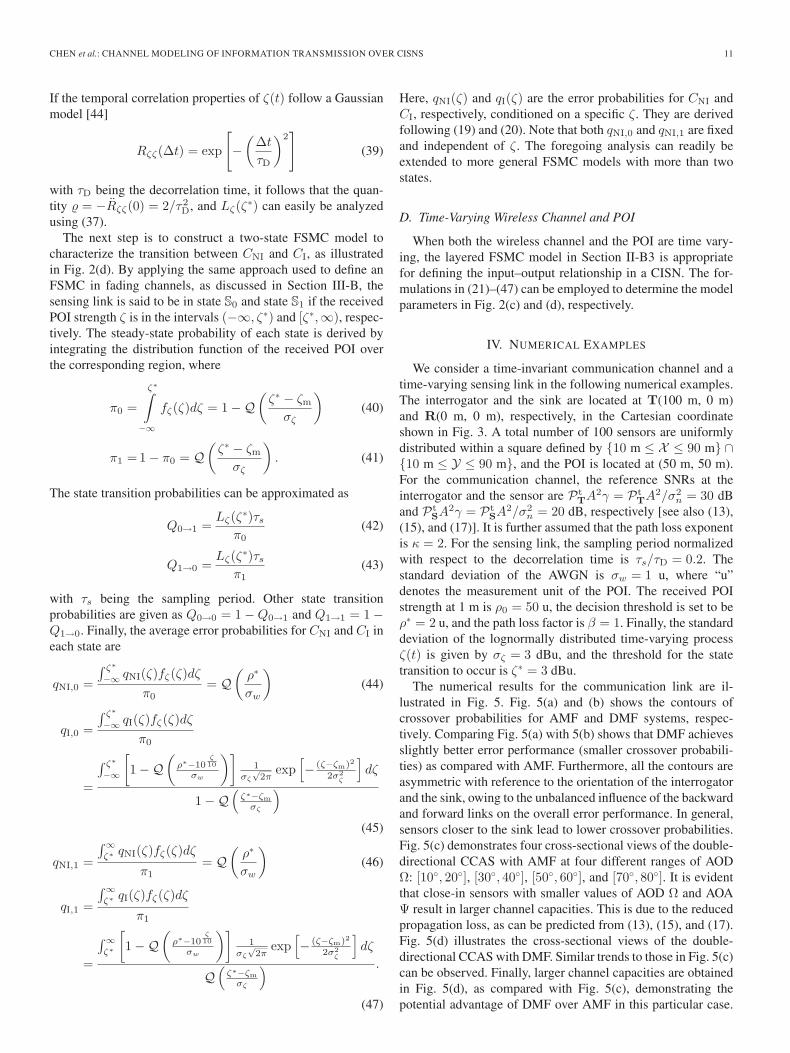
The numerical results for the communication link are il-lustrated in Fig. 5. Fig. 5(a) and (b) shows the contours ofcrossover probabilities for AMF and DMF systems, respec-tively. Comparing Fig. 5(a) with 5(b) shows that DMF achievesslightly better error performance (smaller crossover probabili-ties) as compared with AMF. Furthermore, all the contours areasymmetric with reference to the orientation of the interrogatorand the sink, owing to the unbalanced influence of the backwardand forward links on the overall error performance. In general,sensors closer to the sink lead to lower crossover probabilities.Fig. 5(c) demonstrates four cross-sectional views of the double-directional CCAS with AMF at four different ranges of AODΩ: [10◦, 20◦], [30◦, 40◦], [50◦, 60◦], and [70◦, 80◦]. It is evidentthat close-in sensors with smaller values of AOD Ω and AOAΨ result in larger channel capacities. This is due to the reducedpropagation loss, as can be predicted from (13), (15), and (17).Fig. 5(d) illustrates the cross-sectional views of the double-directional CCAS with DMF. Similar trends to those in Fig. 5(c)can be observed. Finally, larger channel capacities are obtainedin Fig. 5(d), as compared with Fig. 5(c), demonstrating thepotential advantage of DMF over AMF in this particular case.


Fig. 5. Contours of crossover probabilities for the time-invariant commu-nication link. (a) AMF and (b) DMF; cross-sectional views of the double-directional CCAS with (c) AMF and (d) DMF. The legend for (c) and(d) is as follows: ◦ : Ω∈ [10◦, 20◦], × : Ω∈ [30◦, 40◦], +: Ω∈ [50◦, 60◦],� : Ω ∈ [70◦, 80◦].

This also agrees well with the crossover probability data inFig. 5(a) and (b).

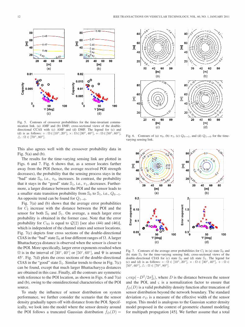
The results for the time-varying sensing link are plotted inFigs. 6 and 7. Fig. 6 shows that, as a sensor locates fartheraway from the POI (hence, the average received POI strengthdecreases), the probability that the sensing process stays in the“bad” state S0, i.e., π0, increases. In contrast, the probabilitythat it stays in the “good” state S1, i.e., π1, decreases. Further-more, a larger distance between the POI and the sensor leads toa smaller state transition probability from S0 to S1, i.e., Q0→1.An opposite trend can be found for Q1→0.

Fig. 7(a) and (b) shows that the average error probabilitiesfor CI increase with the distance between the POI and thesensor for both S0 and S1. On average, a much larger errorprobability is obtained in the former case. Note that the errorprobability for CNI is equal to Q(2) [see also (44) and (46)],which is independent of the channel states and sensor locations.Fig. 7(c) depicts four cross sections of the double-directionalCIAS in the “bad” state S0 at four different ranges of Ω. A largerBhattacharyya distance is observed when the sensor is closer tothe POI. More specifically, larger error exponents resulted whenΩ is in the interval of [30◦, 40◦] or [50◦, 60◦], and Ψ is around45◦. Fig. 7(d) plots the cross sections of the double-directionalCIAS in the “good” state S1. Similar trends to those in Fig. 7(c)can be found, except that much larger Bhattacharyya distancesare obtained in this case. Finally, all the contours are symmetricwith reference to the POI location, as shown in Figs. 6 and 7(a)and (b), owing to the omnidirectional characteristics of the POIsource.

To study the influence of sensor distribution on systemperformance, we further consider the scenario that the sensordensity gradually tapers off with distance from the POI. Specif-ically, we look into the model where the sensor density aroundthe POI follows a truncated Gaussian distribution fD(D) =

Fig. 6. Contours of (a) π0, (b) π1, (c) Q0→1, and (d) Q1→0 for the time-varying sensing link.

Fig. 7. Contours of the average error probabilities for CI in (a) state S0 and(b) state S1 for the time-varying sensing link; cross-sectional views of thedouble-directional CIAS for (c) state S0 and (d) state S1. The legend for(c) and (d) is as follows: ◦ : Ω ∈ [10◦, 20◦], × : Ω ∈ [30◦, 40◦], + : Ω ∈[50◦, 60◦], � : Ω ∈ [70◦, 80◦].

ς exp(−D2/2σ2D), where D is the distance between the sensor

and the POI, and ς is a normalization factor to ensure thatfD(D) is a valid probability density function after truncation ofsensor distribution beyond the network boundary. The standarddeviation σD is a measure of the effective width of the sensorregion. This model is analogous to the Gaussian scatter densitymodel proposed in the context of geometric channel modelingfor multipath propagation [45]. We further assume that a total


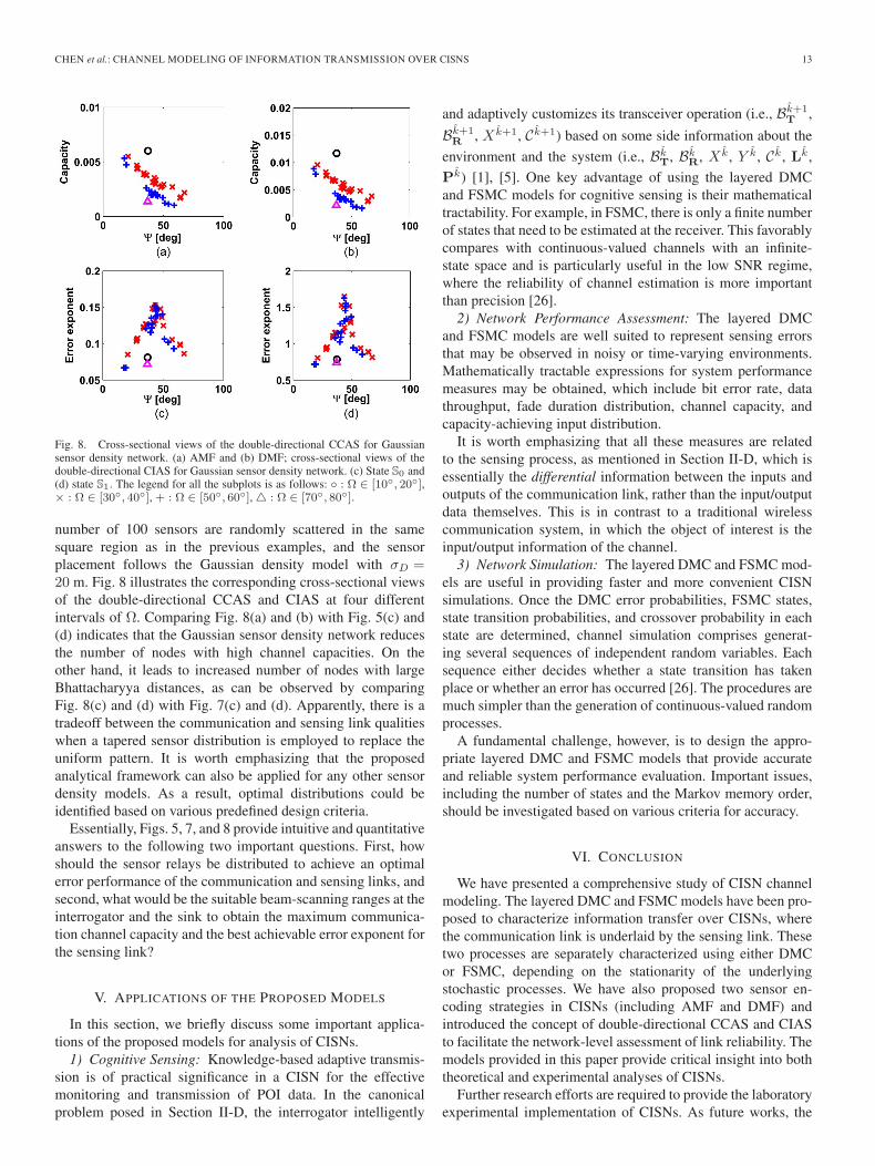
Fig. 8. Cross-sectional views of the double-directional CCAS for Gaussiansensor density network. (a) AMF and (b) DMF; cross-sectional views of thedouble-directional CIAS for Gaussian sensor density network. (c) State S0 and(d) state S1. The legend for all the subplots is as follows: ◦ : Ω ∈ [10◦, 20◦],× : Ω ∈ [30◦, 40◦], + : Ω ∈ [50◦, 60◦], � : Ω ∈ [70◦, 80◦].

number of 100 sensors are randomly scattered in the samesquare region as in the previous examples, and the sensorplacement follows the Gaussian density model with σD =20 m. Fig. 8 illustrates the corresponding cross-sectional viewsof the double-directional CCAS and CIAS at four differentintervals of Ω. Comparing Fig. 8(a) and (b) with Fig. 5(c) and(d) indicates that the Gaussian sensor density network reducesthe number of nodes with high channel capacities. On theother hand, it leads to increased number of nodes with largeBhattacharyya distances, as can be observed by comparingFig. 8(c) and (d) with Fig. 7(c) and (d). Apparently, there is atradeoff between the communication and sensing link qualitieswhen a tapered sensor distribution is employed to replace theuniform pattern. It is worth emphasizing that the proposedanalytical framework can also be applied for any other sensordensity models. As a result, optimal distributions could beidentified based on various predefined design criteria.

Essentially, Figs. 5, 7, and 8 provide intuitive and quantitativeanswers to the following two important questions. First, howshould the sensor relays be distributed to achieve an optimalerror performance of the communication and sensing links, andsecond, what would be the suitable beam-scanning ranges at theinterrogator and the sink to obtain the maximum communica-tion channel capacity and the best achievable error exponent forthe sensing link?

V. APPLICATIONS OF THE PROPOSED MODELS

In this section, we briefly discuss some important applica-tions of the proposed models for analysis of CISNs.

1) Cognitive Sensing: Knowledge-based adaptive transmis-sion is of practical significance in a CISN for the effectivemonitoring and transmission of POI data. In the canonicalproblem posed in Section II-D, the interrogator intelligently

and adaptively customizes its transceiver operation (i.e., Bk̂+1T ,

Bk̂+1R , X k̂+1, Ck̂+1) based on some side information about the

environment and the system (i.e., Bk̂T, Bk̂

R, X k̂, Y k̂, Ck̂, Lk̂,

Pk̂) [1], [5]. One key advantage of using the layered DMCand FSMC models for cognitive sensing is their mathematicaltractability. For example, in FSMC, there is only a finite numberof states that need to be estimated at the receiver. This favorablycompares with continuous-valued channels with an infinite-state space and is particularly useful in the low SNR regime,where the reliability of channel estimation is more importantthan precision [26].

2) Network Performance Assessment: The layered DMCand FSMC models are well suited to represent sensing errorsthat may be observed in noisy or time-varying environments.Mathematically tractable expressions for system performancemeasures may be obtained, which include bit error rate, datathroughput, fade duration distribution, channel capacity, andcapacity-achieving input distribution.

It is worth emphasizing that all these measures are relatedto the sensing process, as mentioned in Section II-D, which isessentially the differential information between the inputs andoutputs of the communication link, rather than the input/outputdata themselves. This is in contrast to a traditional wirelesscommunication system, in which the object of interest is theinput/output information of the channel.

3) Network Simulation: The layered DMC and FSMC mod-els are useful in providing faster and more convenient CISNsimulations. Once the DMC error probabilities, FSMC states,state transition probabilities, and crossover probability in eachstate are determined, channel simulation comprises generat-ing several sequences of independent random variables. Eachsequence either decides whether a state transition has takenplace or whether an error has occurred [26]. The procedures aremuch simpler than the generation of continuous-valued randomprocesses.

A fundamental challenge, however, is to design the appro-priate layered DMC and FSMC models that provide accurateand reliable system performance evaluation. Important issues,including the number of states and the Markov memory order,should be investigated based on various criteria for accuracy.

VI. CONCLUSION

We have presented a comprehensive study of CISN channelmodeling. The layered DMC and FSMC models have been pro-posed to characterize information transfer over CISNs, wherethe communication link is underlaid by the sensing link. Thesetwo processes are separately characterized using either DMCor FSMC, depending on the stationarity of the underlyingstochastic processes. We have also proposed two sensor en-coding strategies in CISNs (including AMF and DMF) andintroduced the concept of double-directional CCAS and CIASto facilitate the network-level assessment of link reliability. Themodels provided in this paper provide critical insight into boththeoretical and experimental analyses of CISNs.

Further research efforts are required to provide the laboratoryexperimental implementation of CISNs. As future works, the


advantages and limitations of the proposed cognitive sensingframework need to be verified by real-life prototypes and exper-imentation. Various designs of RFID sensor tags available in theexisting literature (e.g., multiport tag antennas used as sensors[12], passive chipless RFID sensor system [17], wireless identi-fication and sensing platform [11]) can be applied as sensors inWSNs. Moreover, the integration of a long-range RFID reader[11] and a CR by incorporating an internal feedback loop posesa great design challenge. Eventually, such an integrated systemcan be customized for the realization and empirical testing ofCISNs.

REFERENCES

[1] S. Haykin, “Cognitive radar: A way of the future,” IEEE Signal Process.Mag., vol. 23, no. 1, pp. 30–40, Jan. 2006.

[2] N. A. Goodman, P. R. Venkata, and M. A. Neifeld, “Adaptive waveformdesign and sequential hypothesis testing for target recognition with activesensors,” IEEE J. Sel. Topics Signal Process., vol. 1, no. 1, pp. 105–113,Jun. 2007.

[3] U. Gunturkun, “Toward the development of radar scene analyzer forcognitive radar,” IEEE J. Ocean. Eng., vol. 35, no. 2, pp. 303–313,Apr. 2010.

[4] R. A. Romero and N. A. Goodman, “Waveform design in signal-dependent interference and application to target recognition with multipletransmissions,” IET Radar Sonar Navig., vol. 3, no. 4, pp. 328–340,Aug. 2009.

[5] Y. Chen and P. Rapajic, “Ultra-wideband cognitive interrogator network:Adaptive illumination with active sensors for target localisation,” IETCommun., vol. 4, no. 5, pp. 573–584, Mar. 2010.

[6] D. Culler, D. Estrin, and M. Srivastava, “Overview of sensor networks,”Computer, vol. 37, no. 8, pp. 41–49, Aug. 2004.

[7] B. Krishnamachari, Networking Wireless Sensors. Cambridge, U.K.:Cambridge Univ. Press, 2006.

[8] R. Madan, S. Cui, S. Lall, and A. Goldsmith, “Cross-layer designfor lifetime maximization in interference-limited wireless sensor net-works,” IEEE Trans. Wireless Commun., vol. 5, no. 11, pp. 3142–3152,Nov. 2006.

[9] H. Liu, M. Bolic, A. Nayak, and I. Stojmenovic, “Taxonomy andchallenges of the integration of RFID and wireless sensor networks,”IEEE Netw., vol. 22, no. 6, pp. 26–35, Nov./Dec. 2008.

[10] Y. Chen and W. L. Woo, “On modeling of cognitive interrogator-sensornetwork: Layered discrete memoryless channel and finite-state Markovchannel,” in Proc. 2nd Int. Workshop CIP, Elba Island, Italy, Jun. 2010,pp. 11–16.

[11] M. Philipose, J. R. Smith, B. Jiang, A. Mamishev, S. Roy, and K. SundaraRajan, “Battery-free wireless identification and sensing,” IEEE PervasiveComput., vol. 4, no. 1, pp. 37–45, Jan.–Mar. 2005.

[12] G. Marrocco, L. Mattioni, and C. Calabrese, “Multiport sensor RFIDs forwireless passive sensing of objects—Basic theory and early results,” IEEETrans. Antennas Propag., vol. 56, no. 8, pp. 2691–2702, Aug. 2008.

[13] S. Mandal, L. Turicchia, and R. Sarpeshkar, “A low-power, battery-freetag for body sensor networks,” IEEE Pervasive Comput., vol. 9, no. 1,pp. 71–77, Jan.–Mar. 2010.

[14] C. M. Kruesi, R. J. Vyas, and M. M. Tentzeris, “Design and develop-ment of a novel 3-D cubic antenna for wireless sensor networks (WSNs)and RFID applications,” IEEE Trans. Antennas Propag., vol. 57, no. 10,pp. 3293–3299, Oct. 2009.

[15] A. Vaz, A. Ubarretxena, I. Zalbide, D. Pardo, H. Solar, A. Garcia-Alonso,and R. Berenguer, “Full passive UHF tag with a temperature sensor suit-able for human body temperature monitoring,” IEEE Trans. Circuits Syst.II, Exp. Briefs, vol. 57, no. 2, pp. 95–99, Feb. 2010.

[16] C. Occhiuzzi and G. Marrocco, “The RFID technology for neurosciences:Feasibility of limbs’ monitoring in sleep diseases,” IEEE Trans. Inf. Tech-nol. Biomed., vol. 14, no. 1, pp. 37–43, Jan. 2010.

[17] S. Shrestha, M. Balachandran, M. Agarwal, V. V. Phoha, andK. Varahramyan, “A chipless RFID sensor system for cyber centric mon-itoring applications,” IEEE Trans. Microw. Theory Tech., vol. 57, no. 5,pp. 1303–1309, May 2009.

[18] R. J. M. Vullers, R. V. Schaijk, H. J. Visser, J. Penders, and C. V. Hoof,“Energy harvesting for autonomous wireless sensor networks,” IEEESolid-State Circuits Mag., vol. 2, no. 2, pp. 29–38, Spring 2010.

[19] S. Cheng, K. Tom, L. Thomas, and M. Pecht, “A wireless sensor systemfor prognostics and health management,” IEEE Sensors J., vol. 10, no. 4,pp. 856–862, Apr. 2010.

[20] H. Ramamurthy, B. S. Prabhu, R. Gadh, and A. M. Madni, “Wirelessindustrial monitoring and control using a smart sensor platform,” IEEESensors J., vol. 7, no. 5, pp. 611–618, May 2007.

[21] F. Hu, Y. Xiao, and Q. Hao, “Congestion-aware, loss-resilient bio-monitoring sensor networking for mobile health applications,” IEEE J.Sel. Areas Commun., vol. 27, no. 4, pp. 450–465, May 2009.

[22] P.-Y. Chen, W.-T. Chen, Y.-C. Tseng, and C.-F. Huang, “Providing grouptour guide by RFIDs and wireless sensor networks,” IEEE Trans. WirelessCommun., vol. 8, no. 6, pp. 3059–3067, Jun. 2009.

[23] J. Cho, Y. Shim, T. Kwon, Y. Choi, S. Pack, and S. Kim, “SARIF: Anovel framework for integrating wireless sensor and RFID networks,”IEEE Wireless Commun., vol. 14, no. 6, pp. 50–56, Dec. 2007.

[24] C.-X. Wang, H.-H. Chen, X. Hong, and M. Guizani, “Cognitive radio net-work management: Tuning into real-time conditions,” IEEE Veh. Technol.Mag., vol. 3, no. 1, pp. 28–35, Mar. 2008.

[25] C.-X. Wang, X. Hong, H.-H. Chen, and J. S. Thompson, “On capac-ity of cognitive radio networks with average interference power con-straints,” IEEE Trans. Wireless Commun., vol. 8, no. 4, pp. 1620–1625,Apr. 2009.

[26] P. Sadeghi, R. A. Kennedy, P. B. Rapajic, and R. Shams, “Finite-stateMarkov modeling of fading channels,” IEEE Signal Process. Mag.,vol. 25, no. 5, pp. 57–80, Sep. 2008.

[27] H. S. Wang and N. Moayeri, “Finite-state Markov channel—A usefulmodel for radio communication channels,” IEEE Trans. Veh. Technol.,vol. 44, no. 1, pp. 163–171, Feb. 1995.

[28] C.-X. Wang and W. Xu, “A new class of generative models for burst errorcharacterization in digital wireless channels,” IEEE Trans. Commun.,vol. 55, no. 3, pp. 453–462, Mar. 2007.

[29] J. N. Laneman, D. N. C. Tse, and G. W. Wornell, “Cooperative diversity inwireless networks: Efficient protocols and outage behavior,” IEEE Trans.Inf. Theory, vol. 50, no. 12, pp. 3062–3080, Dec. 2004.

[30] C. S. Patel, G. L. Stüber, and T. G. Pratt, “Statistical properties of amplifyand forward relay fading channels,” IEEE Trans. Veh. Technol., vol. 55,no. 1, pp. 1–9, Jan. 2006.

[31] R. U. Nabar, H. Boelcskei, and F. W. Kneubhueler, “Fading relay chan-nels: Performance limits and space-time signal design,” IEEE J. Sel. AreasCommun., vol. 22, no. 6, pp. 1099–1109, Aug. 2004.

[32] C.-X. Wang, X. Hong, X. Ge, X. Cheng, G. Zhang, and J. S. Thompson,“Cooperative MIMO channel models: A survey,” IEEE Commun. Mag.,vol. 48, no. 2, pp. 80–87, Feb. 2010.

[33] C. C. Y. Poon, Y. T. Zhang, and S. D. Bao, “A novel biometricsmethod to secure wireless body area sensor networks for telemedicine andm-health,” IEEE Commun. Mag., vol. 44, no. 4, pp. 73–81, Apr. 2006.

[34] R. G. Gallager, Principles of Digital Communication. Cambridge, U.K.:Cambridge Univ. Press, 2008.

[35] J.-F. Chamberland and V. V. Veeravalli, “Decentralized detection in sensornetworks,” IEEE Trans. Signal Process., vol. 51, no. 2, pp. 407–416,Feb. 2003.

[36] A. Leshem, O. Naparstek, and A. Nehorai, “Information theoretic adaptiveradar waveform design for multiple extended targets,” IEEE J. Sel. TopicsSignal Process., vol. 1, no. 1, pp. 42–55, Jun. 2007.

[37] A. Ishimaru, Wave Propagation and Scattering in Random Media.Oxford, U.K.: Oxford Univ. Press, 1997.

[38] T. M. Cover and J. A. Thomas, Elements of Information Theory.New York: Wiley, 1991.

[39] R. G. Gallager, Information Theory and Reliable Communications.New York: Wiley, 1968.

[40] Y. Chen and P. Rapajic, “Decentralized wireless relay network chan-nel modeling: An analogous approach to mobile radio channelcharacterization,” IEEE Trans. Commun., vol. 58, no. 2, pp. 467–473,Feb. 2010.

[41] A. F. Molisch, Wireless Communications. Chichester, U.K.: Wiley,2005.

[42] S. R. Saunders and A. Aragon-Zavala, Antennas and Propagation forWireless Communication Systems. Chichester, U.K.: Wiley, 2007.

[43] T. Q. S. Quek, D. Dardari, and M. Z. Win, “Energy efficiency of densewireless sensor networks: To cooperate or not to cooperate,” IEEE J. Sel.Areas Commun., vol. 25, no. 2, pp. 459–470, Feb. 2007.

[44] M. Patzold and K. Yang, “An exact solution for the level-crossing rate ofshadow fading processes modelled by using the sum-of-sinusoids princi-ple,” Wireless Pers. Commun., vol. 52, no. 1, pp. 57–68, Jan. 2010.

[45] R. Janaswamy, “Angle and time of arrival statistics for the Gaussianscatter density model,” IEEE Trans. Wireless Commun., vol. 1, no. 3,pp. 488–497, Jul. 2002.


Yifan Chen (M’06) received the B.Eng. (Hons. I)and Ph.D. degrees in electrical and electronic en-gineering from Nanyang Technological University(NTU), Singapore, in 2002 and 2006, respectively.

From 2005 to 2007, he was a Research Fellowwith the Singapore-University of Washington Al-liance in Bioengineering, NTU. From 2007 to 2010,he was a Senior Lecturer with the School of Engi-neering, University of Greenwich, London, U.K. Heis currently a Lecturer with the School of Electrical,Electronic, and Computer Engineering, Newcastle

University, Newcastle upon Tyne, U.K. He is also an Adjunct AssociateProfessor with the School of Computer, Electronics, and Information, GuangxiUniversity, Nanning, China. His current research interests involve wirelessand pervasive communications for healthcare, microwave biomedical imaging,wireless channel modeling, wireless communication theory, and cognitivedynamic systems.

Dr. Chen received the Promising Research Fellowship in 2010 and theEarly Career Research Excellence Award in 2009 from the University ofGreenwich in recognition of his exceptional research contributions andpotential.

Wai Lok Woo was born in Malaysia. He received theB.Eng. degree (First-Class Hons.) in electrical andelectronics engineering and the Ph.D. degree fromNewcastle University, Newcastle upon Tyne, U.K.

He is currently a Senior Lecturer with the Schoolof Electrical, Electronic, and Computer Engineering,Newcastle University. He currently serves on theeditorial boards of many international signal process-ing journals. He actively participates in internationalconferences and workshops and serves on their orga-nizing and technical committees. In addition, he acts

as a Consultant to a number of industrial companies that involve the use ofstatistical signal processing techniques. His major research is in mathematicaltheory and algorithms for nonlinear signal processing. This includes areas ofblind signal separation, signal characterization and identification, information-theoretic learning, deconvolution, and restoration.

Dr. Woo received the IEE Prize and the British Scholarship in 1998 tocontinue his research.

Cheng-Xiang Wang (S’01–M’05–SM’08) receivedthe B.Sc. and M.Eng. degrees in communicationand information systems from Shandong University,Jinan, China, in 1997 and 2000, respectively, andthe Ph.D. degree in wireless communications fromAalborg University, Aalborg, Denmark, in 2004.

He was a Research Assistant with the Tech-nical University of Hamburg-Harburg, Hamburg,Germany, from 2000 to 2001, a Research Fellowwith the University of Agder, Grimstad, Norway,from 2001 to 2005, and a Visiting Researcher with

Siemens AG-Mobile Phones, Munich, Germany, in 2004. He is an HonoraryFellow of the University of Edinburgh, Edinburgh, U.K., a Chair Professor ofShandong University, a Guest Professor of the Huazhong University of Scienceand Technology, Wuhan, China, an Adjunct Professor of Guilin Universityof Electronic Technology, Guilin, China, and a Guest Researcher of XidianUniversity, Xi’an, China. He has been with Heriot-Watt University, Edinburgh,since 2005, first as a Lecturer and then as a Reader in 2009. He is leadingseveral projects funded by the Engineering and Physical Sciences ResearchCouncil (EPSRC), Mobile VCE, and industries, including the Research Coun-cils UK funded “U.K.-China Science Bridges: R&D on (B)4G Wireless MobileCommunications.” He has published one book chapter and about 140 papersin refereed journals and conference proceedings. He is currently serving asEditor for Wireless Communications and Mobile Computing Journal (Wiley),the Security and Communication Networks Journal (Wiley), and the Journalof Computer Systems, Networks, and Communications (Hindawi). His currentresearch interests include wireless channel modeling and simulation, cogni-tive radio networks, vehicular communication networks, green radio com-munications, cooperative multiple-input–multiple-output, cross-layer designof wireless networks, utra-wideband, and beyond fourth-generation wirelesscommunications.

Dr. Wang is a member of the Institution of Engineering and Technology(IET), a Fellow of the High Education Academy (HEA), and a member ofthe EPSRC Peer Review College. He served as Editor for the IEEE TRANS-ACTIONS ON WIRELESS COMMUNICATIONS from 2007 to 2009. He is theleading Guest Editor for the IEEE JOURNAL ON SELECTED AREAS IN COM-MUNICATIONS Special Issue on Vehicular Communications and Networks. Heserved or is serving as Technical Program Committee (TPC) member, TPCChair, and General Chair for about 60 international conferences. He receivedthe Best Paper Award at the IEEE Global Communications Conference in 2010.He is listed in the “Dictionary of International Biography 2008 and 2009,”“Who’s Who in the World 2008 and 2009,” “Great Minds of the 21st Century2009,” and “2009 Man of the Year.”

Documents

Channel Modeling of Information ... - home.eps.hw.ac.uk