Channel Mobility Incurred Source Routing in

Cognitive Radio Networks

Yupeng Li, Boya PengDepartment of Computer Science,

University of Hong Kong

November 1, 2014

Abstract

In Cognitive Radio Networks (CRN), Secondary users are allowed touse Primary Users’ (PUs’) idle channels for data transmission. However,PUs can reclaim their channels at any time and SUs must cease trans-mission immediately. Such a problem is known as the spectrum mobility,and may further cause break of pre-established routes in multi-hop CRNswhere SUs act as relays. In this paper, we investigate a routing problemwhere channel switching and route re-selection are deployed to resolveSUs’ conflicts with PUs and further improve spectrum mobility. In par-ticular, we consider both protocol and physical interference models andform the routing game into a routing game which is proved to be a po-tential game with a pure Nash Equilibrium (NE). Finally, we present anefficient algorithm for finding the NE and analyze the Price of Stabilityof the proposed game.

1 Introduction

Wireless spectrum is currently regulated by government and is assigned to li-cense holders and services on a long term basis. However, a large portion ofthe assigned spectrum is used sporadically, which leads to under utilization offrequency resources.The problem foresees the development of Cognitive RadioNetworks (CRNs) to improve spectrum efficiency. The idea of CRN is that unli-censed users (Secondary Users, SUs) can flexibly access licensed users’ (PrimaryUsers, PUs) idle channels without interfering with other PUs’ transmission.While such Dynamic Spectrum Access (DSA) improves spectrum utilization,new problems such as spectrum sensing, channel selection, MAC and routingprotocols design occurred with regard to the architecture of CRNs, and one ofthe major problems is spectrum mobility.

In CRNs, due to higher priorities, PUs are allowed to reclaim their licensedchannels at any time, while SUs must cease their transmissions immediately.Therefore, for multi-hop CRNs where SUs act as relays, spectrum mobility may

1

break pre-established routes as it disables data transmission over certain linkson those routes. To avoid conflicts with PUs and resume routing, each flowgenerator can either inform intermediate SUs to switch channels or select a newroute. However, there is no clear answer as for which approach is better. Whileswitching channels keeps the original spacial routes which effectively reducerouting costs, frequent channel switching may cause significant switching costs.On the other hand, while re-selecting a spacial route can reduce switching costs,it may result in additional routing costs in the mean time. Therefore, due tothe trade off between channel switching and route re-selection, we combine thetwo approaches into a routing problem as a whole.

In this paper, we construct the routing problem into a routing game, whereeach flow generator acts as a player and selects its route selfishly to minimizeits own cost, which results from both channel switching and route re-selection.In particular, we pay attention to the scenario where multiple flows can sharea common link which further improves spectrum efficiency but introduces con-gestion costs. Furthermore, we consider both protocol and physical interferencemodels, and construct the cost model and form the game accordingly.

The contributions of this paper include the following:

• We formulate the problem as the Route-Switching Game.

• We construct the game in regards to both protocol and physical interfer-ence models.

• We prove the existence of Nash Equilibria (NE) by applying the OrdinalPotential Game method

• We simulate the Fictitious Play Process as the learning algorithm for thegame, prove its feasibility and efficiency, and analyze the Price of Stability(PoS).

The rest of this paper is organized as following: We will first introduce somerelated works in section 2 and present the system model in section 3. Then insection 4, game formation for the Routing Game will be discusses. Next, weanalyze the learning strategy for the game and the Price of Anarchy in section5 and 6. At last, we present simulation results and conclusion in section 7 and8 respectively.

2 Related Works

For routing problem in multi-hop CRN, the most relevant work would be thetwo dimensional routing game proposed by Qingkai [1], which also exploreda joint scheme of channel switching and routing re-selection in the context ofspectrum-mobility incurred route-switching problem in multi-hop CRN. How-ever, his work failed to consider the scenario where multiple flows sharing acommon link, and he considered only the protocol interference model but notthe physical interference model. Most of the other works only considered either

2

channel switching or spatial route selection. For instance, Qinghai [2] proposeda proactive channel selection scheme based on spectrum hole prediction. Heintroduced two two opportunistic channel selection algorithms to optimize thethroughput of the secondary user: minimum collision rate channel selection algo-rithm and minimum handoff rate channel selection algorithm. Besides, Zhao [3]provided a robust channel assignment scheme in the multi-hop CRN, while Cal-effi [4] proposed the criterion for an optimal routing metric in CRNs based onthe diversity effects of spatial routes.

As for game formation, Roughgarden [5, p. 461- 487] discussed selfish routinggame in general, and analyzed the existence and uniqueness of a Nash Equilib-rium (NE) in the game. He then introduced the potential function method forfinding NE, and brought up the concept of the Price of Stability (PoS) whichcompare the best NE to the socially optimal result to analyze the efficiencyof self routing games. Furthermore, Ragavendran [6] discussed the ’hourglass’architecture for game-theoretic control, which allowed a diverse set of possibleutility and learning designs, with an constrained interface connecting the two.In this paper, we construct players’ utility function in terms of routing costs,and deploy the famous Fictitious Play (FP) process [7] as the learning rulefor each player to update its strategy during the game. Additionally, the classpotential game is chosen to be the constrained interface, which requires utilitydesigns to guarantee that the resulting game is a potential game and requiredlearning rules to guarantee to provide desirable behavior. In a potential game,a pure Nash Equilibrium will be reached where no player can further reduce itsown cost under the specific utility and learning design.

3 System Model

What we consider is the channel-mobility-incurred source routing problem inthe multi-flow multi-hop Cognitive Radio Networks (CRNs). In this section, wepresent the formal definitions of our system model.

3.1 Cognitive Radio Networks (CRNs)

A CRN can be characterized by a potential directed graph G = (V,E), where Vis the set of all active secondary users in the network and E denotes the set ofall potential links. Here, potential links mean that not all the links in this graphcan be established simultaneously. Similar to other recent works on CRNs, weonly consider unicast in the communication, and assume that each node hasalready had a stable power level1. Therefore, with a known power level, we canget the wireless transmission range of each node and establish all the potentiallinks. Formally, an edge eci(u,v) ∈ E from SUu to SUv is established if and onlyif SUv is within the transmission range of SUu, which is a potential link andtherefore corresponds with a channel c. We assume that a node can be equipped

1Broadcast and power allocation is beyond our consideration here.

3

with multiple antennae2, so multiple wireless links can be established betweentwo nodes. Two links are called opposite if they differ from each other only bythe direction, and are denoted e and e.

3.2 Channel

In CRNs, each secondary user (SU) is able to sense the licensed channel stateto avoid colliding with any PU who has the priority to occupy channels. Eachuser3 can establish a link with any SU within its own transmission range on anychannel they have sensed. We denote C = {1, 2, . . . , C} as the potential availablechannel set, and CSUi

is the available4 channel set of the ith SU at a time. Sincemost channels in CRNs are occupied by PUs, C is a small number, and we canassume that the number of antennae of each wireless node is enough to supportall its potential links working on different available channels simultaneously.Since different SU may collide with different PUs, CSUi

and CSUjcan be not

equal given that i 6= j at a time.

3.3 Flow

There are N flows indicated by i ∈ N = {1, 2, ..., N} being injected into thenetwork concurrently, each of which can be considered being generated by anunique fictitious flow generator. That is to say, no two flows are from the samegenerator. Each flow corresponds to a source-destination pair (s, t) and has anumber of information (packets) to transmit. For example, flow i has to routeits αi information from si to ti in one period of time5. We assume that 1) theinformation can be divided into equal size to transmit no matter which flowthey belong to; 2) each flow generator chooses only one path to route all itsinformation; 3)the buffer at each node is large enough to sustain the wholeprocess.

3.4 Interference and Congestion

We deploy a linear interference measurement to generalize different kinds ofinterference model. We use a matrix I to characterize the influence of thetransmission on one link on a transmission of another link. For links eci(u,v) and

ec′

j(u′,v′), I(i, j) shows to what extent link eci(u,v) is interfered by link ec′

j(u′,v′) at a

time. Note that only the link pairs assigned with the same channel (c = c′) caninterfere with each other, for the ones assigned with different channels (c 6= c′),the corresponding entries are set to zero. After normalization, 0 ≤ I(i, j) ≤ 1

2i stands for link’s (or edge’s) identity; u, v stand for the nodes; and c stands for a channel.We will use eci , ei and e for denoting simplicity according to the context, all of which areliterally equivalent to ec

i(u,v).

3We will use secondary user, user, SU and node interchangeably in this draft.4”Available” means that the channel is sensed idle, and can be used by the user.5In this paper, we consider the concurrent flows. Each generator will choose a route

periodically. In each period of time, αi information are expected to route.

4

for any ei, ej ∈ E. In particular, we set I(i, j) = 1 for any two links eci(u,v) andecj(v,u) between two nodes that are assigned with the same channel but have

opposite directions; the special case, I(i, i) = 1, is included, which denotes thecongestion on this link (we will specify on it later). As for the other entries,the value will depend on the interference model we adopt. Two most frequentlyused models, the protocol model and the physical SINR model, are considered.

• Protocol interference model. Each entry of I is either 1 or 0. That is,for link pair ei, ej ∈ E, I(ei, ej) = 1 if and only if ei and ej are as-signed with the same channel and ei is within the interference range ofej

6, and I(ei, ej) = 0 otherwise. The restriction in this model is that somenearby links may share a channel but only one link can support a success-ful transmission over this channel at one time. That is, for a successfultransmission on link ei, the constraint is∑

ej∈E\{ei}

I(ei, ej) · Z(ej) = 0, (1)

where Z(ej) = 1 if and only if ej is activated, i.e., included in at leastone path that is routed by at least one flow at a time, and Z(ej) = 0otherwise.

• Physical interference model. For two links eci(u,v) and ecj(p,q), I(eci , ecj)

indicates how much a transmission on ecj interfere with a transmission oneci , i.e., the ratio of the signal power at receiver SUv from SUp to thatfrom SUu. Specifically, we set I(eci , e

cj) = +∞ for any wireless link ecj

which has the receiver of eci as its sender in the same channel c, since onenode cannot send and receive information simultaneously at one channel.Under the SINR model, the constraint for a successful transmission onlink eci is ∑

ej∈E\{ei}

I(ei, ej) · Z(ej) ≤1

β, (2)

where β is the threshold in the model, and we ignore the ambient noise.

Note that the above matrix can be established when the topology informationand the interference model are known, with the assumption that the power levelof each wireless device is stable.

3.5 Assumptions

We list following important assumptions that are related to our studies.

Assumption 1. Each flow generator can only select one path between its ownsource-destination node pair to route all its information. Under the interferenceconstraint of a interference model, for each flow i, there exists at least one

6For example, the sender of ej can interfere with the receiver of ei.

5

feasible path from si to ti, regardless of other flows’ choices of strategies. Andeach secondary user will honestly follow the routing strategies developed by flowgenerators.

Assumption 2. At one (short) period of time, the channel states, the topologyof CRNs and flows information including the source-destination pair and theexpected number of information to be transmitted are known to each fictitiousflow generator.

Assumption 3. The injection rate7 of each flow is high enough to support thecontinuity of the routing process. That is, there will always be some informationarriving at the source node ready for transmission, and the source node will notbe idle unless the last packet of the related flow has been sent out.

We find that a reasonable injection rate (i.e., the upper bound of it) has beenissued by the researchers. And it can vary based on different assumptions ofstochastic environment. However, this is beyond our concerns, so we just needto guarantee that it won’t be too low.

Assumption 4. Any channel is not allowed to be used by any PU and anySU simultaneously, even when interference is not high enough to break the linksbetween PUs.

Assumption 5. (”Backoff”) Whenever a channel reclaimation occurs, all in-termediate nodes drop the undelivered packets and the source nodes re-transmitthe packets whose ACK is not received.

4 Game Formulation

In this section, we formulate a routing and switching game in a cognitive radionetwork, which is asymmetric and non-identical-interest (selfish), consideringthat each flow comes from different application with selfish nature as statedabove. Both the protocol interference model and the physical interference modelare considered. We first introduce the cost of a link that a flow pays for whenrouting through it by specifying the components that constitute the link costto illustrate the impacts on the performance of routing. Then, path cost isintroduced, based on which a flow determines its path to route its packets.Finally, we formulate the game that corresponds to the routing problem.

4.1 Link Cost

We now present the cost of a link when a flow selects it to route its packets, whichinstructs each flow generator to choose its path. For the ith flow, set Pi as the setof its possible routing strategies. Only one path pki ∈ Pi is chosen to route all itspackets for any i ∈ {1, 2, ..., N} and k ∈ {1, 2, ..., |Pi|}. Let P =

⋃i∈N Pi, which

is the union of all the possible routing paths for the N flows. The strategies of

7Here, injection rate corresponds to the receiving rate that the source node perceived.

6

all the N flows are within the space P = P1×P2×· · ·×PN , where a dimensionPi = Pi. According to Assumption 1, for each flow i, there exists at least onefeasible path from si to ti regardless of other flows’ strategies.

We employ a two-dimensional matrix XNP to denote the path selection ofeach flow, where Xi

p = 1 if the ith flow chooses path p. Similarly, for any

link e ∈ E, set Xie = 1 if this link is selected by the ith flow, which means

e ∈ p and Xip = 1 (p ∈ Pi). Since self-impact can be reduced by some modern

transmission technology, any self-impact (e.g. congestion and interference) isassumed to be ignored. We denote Qi(e) as the expected number of packetsof all the other flows rather than the ith flow that will be transmitted on edgee ∈ E in a period of time. Denote αi as the expected number of packets thatthe ith flow will transmit over e during the same period of time. And we canhave

Qi(e) =∑j∈Ni

∑p∈P & e∈p

Xjp · αj =

∑j∈Ni

Xje · αj , (3)

where Ni := N \ {i}.For link e : Xi

e = 1, the cost for flow i routing its packets on link e ischaracterized as follows, which includes the congestion cost, the interferencecost, the switching cost and the the energy cost.

4.1.1 Congestion

Since we allow routing multiple flows on one link, there may exist congestion.Congestion that caused by different flows transmitting packets on the same linkor on the links that have the opposite directions8. Recall that for flow i, Qi(e)and Qi(e) denote the expected number of packets of other flows transmittingon link e and its opposite link e in a period of time, respectively. We utilizea cost function to formulate the congestion cost of flow i on edge e, denotedas D(i, e) = λ(I(e, e)Qi(e), I(e, e)Qi(e)). λ(x, y) is a non-decreasing functionof either x (with y fixed) or y (with x fixed). The cost function implies thatthe link will get more congested when the number of packets transmitted on itincreases. We can see that the congestion link cost reflects the queuing delay inthe cognitive radio networks.

4.1.2 Interference

Assigning a pair of links with the same channel incurs interference. Interferencewill lead to a fall in transmission rate no matter which interference model istaken into consideration. We have defined Matrix I to denote the interferencerelationship between any two of the potential communication links. So, we canformulate the interference cost under each of the two interference models witha cost function as follows.

8This has been discussed above (i.e., I(e, e) = 1). In this case, wireless links are assignedwith the same channel but have opposite directions. We will use the term ”opposite links” todenote this case.

7

• For the protocol interference model, we consider a CSMA-like contentioncost. In this contention protocol, one link that is interfered by some otherlinks will contend for transmission since only one of them can transmit suc-cessfully at one time. We model the interference link cost as the expectedcontention delay, as follows.

F1(i, e) = µ1(Mi(e)−D(i, e)),∀e ∈ E (4)

where Mi = I ·Qi is a vector. And µ1(·) is a non-decreasing function.

• For the physical interference model, we have

F2(i, e) =

µ2(Mi(e)−D(i, e)), ∀e ∈ E&IF ≤ 1

β

0, otherwise(5)

where IF =∑e′∈E\{e} I(e, e′) · Zi(e′). Zi(e) denotes whether some flows

other than the ith one select the path including link e, since we ignorethe impact of one’s own transmission on itself. The inequality IF ≤ 1

β

corresponds to the condition for a successful transmission on a link (seeFormula (2)). µ2(·) is a non-decreasing function. The expected amountof packets transmitting on the link that interferes with link e implies itsactive time.

4.1.3 Switching

Since a switching operation may cause delay and energy consumption, we splitswitching cost into two parts, one is the switching delay cost, and the other isthe switching energy cost. Similar to the related works, we introduce a binaryvector H to store the pre-established links. Formally, He = 1 implies that linke was pre-established (but may be broken now as the channel assigned on it isreclaimed by PUs or for other reasons) and He = 0 otherwise. Note that theswitching cost of one link is shared by all the flows routed on it. The switchingdelay cost of flow i on link e is given by

Ga(i, e) =αiQ(e)

· ν · (1−He) ·Xie (6)

where ν is a constant number denoting the unit switching delay cost.The switching energy cost of flow i on link e is given by

Gb(i, e) =αiQ(e)

· ξ · (1−He) ·Xie (7)

where ξ is a constant number denoting the unit energy cost per switching oper-ation.

We denote G(i, e) as the total switching cost, which is a function of thecombination of Ga(i, e) and Gb(i, e).

8

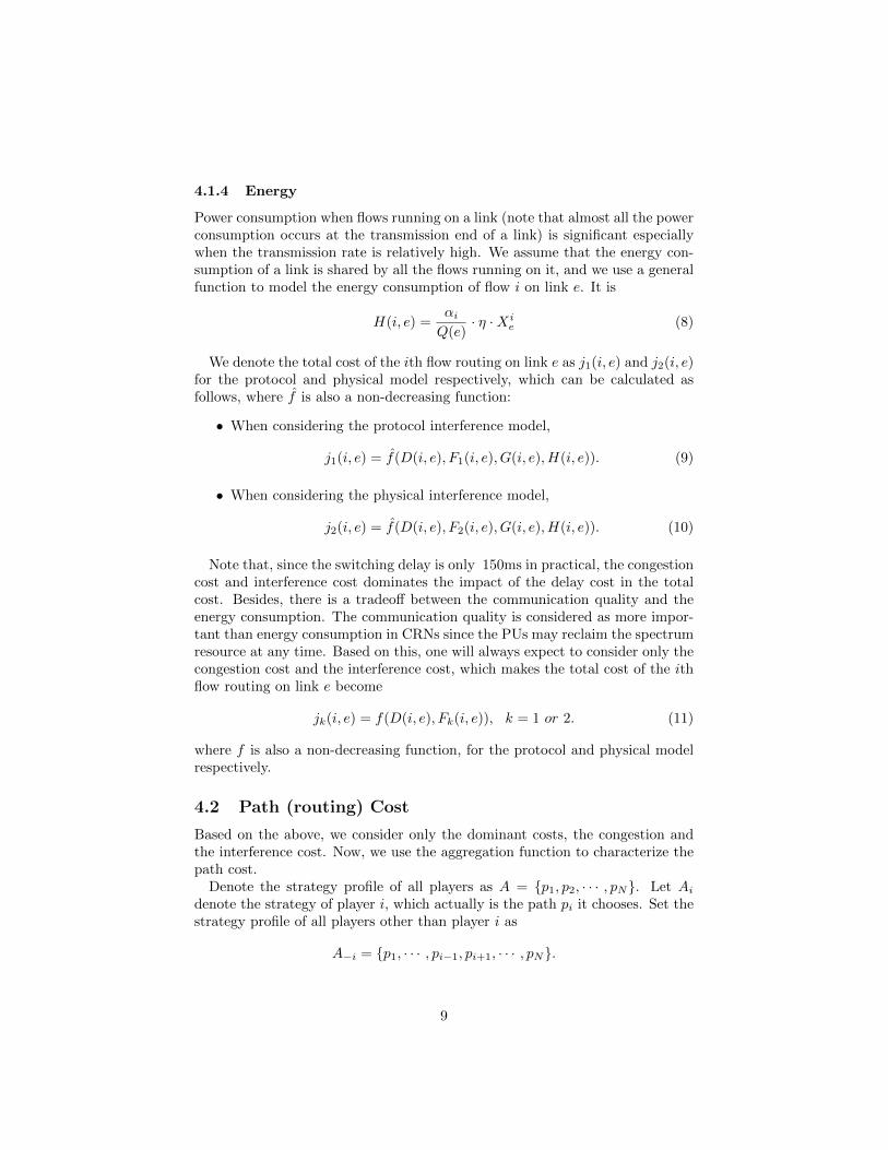
4.1.4 Energy

Power consumption when flows running on a link (note that almost all the powerconsumption occurs at the transmission end of a link) is significant especiallywhen the transmission rate is relatively high. We assume that the energy con-sumption of a link is shared by all the flows running on it, and we use a generalfunction to model the energy consumption of flow i on link e. It is

H(i, e) =αiQ(e)

· η ·Xie (8)

We denote the total cost of the ith flow routing on link e as j1(i, e) and j2(i, e)for the protocol and physical model respectively, which can be calculated asfollows, where f is also a non-decreasing function:

• When considering the protocol interference model,

j1(i, e) = f(D(i, e), F1(i, e), G(i, e), H(i, e)). (9)

• When considering the physical interference model,

j2(i, e) = f(D(i, e), F2(i, e), G(i, e), H(i, e)). (10)

Note that, since the switching delay is only 150ms in practical, the congestioncost and interference cost dominates the impact of the delay cost in the totalcost. Besides, there is a tradeoff between the communication quality and theenergy consumption. The communication quality is considered as more impor-tant than energy consumption in CRNs since the PUs may reclaim the spectrumresource at any time. Based on this, one will always expect to consider only thecongestion cost and the interference cost, which makes the total cost of the ithflow routing on link e become

jk(i, e) = f(D(i, e), Fk(i, e)), k = 1 or 2. (11)

where f is also a non-decreasing function, for the protocol and physical modelrespectively.

4.2 Path (routing) Cost

Based on the above, we consider only the dominant costs, the congestion andthe interference cost. Now, we use the aggregation function to characterize thepath cost.

Denote the strategy profile of all players as A = {p1, p2, · · · , pN}. Let Aidenote the strategy of player i, which actually is the path pi it chooses. Set thestrategy profile of all players other than player i as

A−i = {p1, · · · , pi−1, pi+1, · · · , pN}.

9

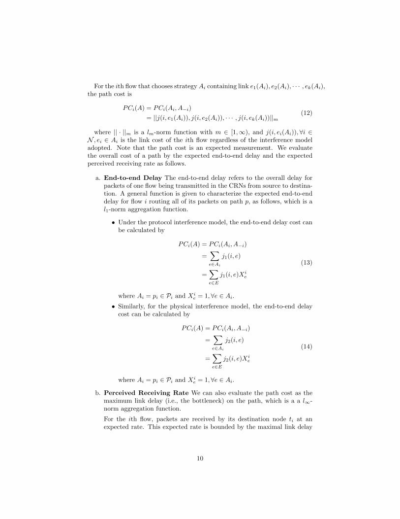
For the ith flow that chooses strategyAi containing link e1(Ai), e2(Ai), · · · , ek(Ai),the path cost is

PCi(A) = PCi(Ai, A−i)

= ||j(i, e1(Ai)), j(i, e2(Ai)), · · · , j(i, ek(Ai))||m(12)

where || · ||m is a lm-norm function with m ∈ [1,∞), and j(i, ei(Ai)),∀i ∈N , ei ∈ Ai is the link cost of the ith flow regardless of the interference modeladopted. Note that the path cost is an expected measurement. We evaluatethe overall cost of a path by the expected end-to-end delay and the expectedperceived receiving rate as follows.

a. End-to-end Delay The end-to-end delay refers to the overall delay forpackets of one flow being transmitted in the CRNs from source to destina-tion. A general function is given to characterize the expected end-to-enddelay for flow i routing all of its packets on path p, as follows, which is al1-norm aggregation function.

• Under the protocol interference model, the end-to-end delay cost canbe calculated by

PCi(A) = PCi(Ai, A−i)

=∑e∈Ai

j1(i, e)

=∑e∈E

j1(i, e)Xie

(13)

where Ai = pi ∈ Pi and Xie = 1,∀e ∈ Ai.

• Similarly, for the physical interference model, the end-to-end delaycost can be calculated by

PCi(A) = PCi(Ai, A−i)

=∑e∈Ai

j2(i, e)

=∑e∈E

j2(i, e)Xie

(14)

where Ai = pi ∈ Pi and Xie = 1,∀e ∈ Ai.

b. Perceived Receiving Rate We can also evaluate the path cost as themaximum link delay (i.e., the bottleneck) on the path, which is a a l∞-norm aggregation function.

For the ith flow, packets are received by its destination node ti at anexpected rate. This expected rate is bounded by the maximal link delay

10

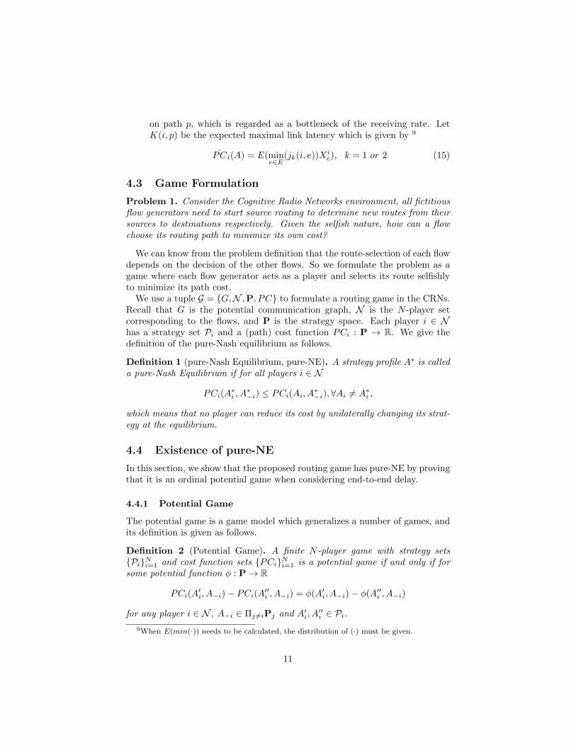
on path p, which is regarded as a bottleneck of the receiving rate. LetK(i, p) be the expected maximal link latency which is given by 9

PCi(A) = E(mine∈E

(jk(i, e))Xie), k = 1 or 2 (15)

4.3 Game Formulation

Problem 1. Consider the Cognitive Radio Networks environment, all fictitiousflow generators need to start source routing to determine new routes from theirsources to destinations respectively. Given the selfish nature, how can a flowchoose its routing path to minimize its own cost?

We can know from the problem definition that the route-selection of each flowdepends on the decision of the other flows. So we formulate the problem as agame where each flow generator acts as a player and selects its route selfishlyto minimize its path cost.

We use a tuple G = {G,N ,P, PC} to formulate a routing game in the CRNs.Recall that G is the potential communication graph, N is the N -player setcorresponding to the flows, and P is the strategy space. Each player i ∈ Nhas a strategy set Pi and a (path) cost function PCi : P → R. We give thedefinition of the pure-Nash equilibrium as follows.

Definition 1 (pure-Nash Equilibrium, pure-NE). A strategy profile A∗ is calleda pure-Nash Equilibrium if for all players i ∈ N

PCi(A∗i , A

∗−i) ≤ PCi(Ai, A∗−i),∀Ai 6= A∗i ,

which means that no player can reduce its cost by unilaterally changing its strat-egy at the equilibrium.

4.4 Existence of pure-NE

In this section, we show that the proposed routing game has pure-NE by provingthat it is an ordinal potential game when considering end-to-end delay.

4.4.1 Potential Game

The potential game is a game model which generalizes a number of games, andits definition is given as follows.

Definition 2 (Potential Game). A finite N -player game with strategy sets{Pi}Ni=1 and cost function sets {PCi}Ni=1 is a potential game if and only if forsome potential function φ : P→ R

PCi(A′i, A−i)− PCi(A′′i , A−i) = φ(A′i, A−i)− φ(A′′i , A−i)

for any player i ∈ N , A−i ∈ Πj 6=iPj and A′i, A′′i ∈ Pi.

9When E(min(·)) needs to be calculated, the distribution of (·) must be given.

11

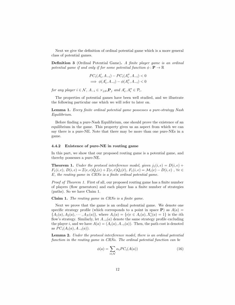
Next we give the definition of ordinal potential game which is a more generalclass of potential games.

Definition 3 (Ordinal Potential Game). A finite player game is an ordinalpotential game if and only if for some potential function φ : P→ R

PCi(A′i, A−i)− PCi(A′′i , A−i) < 0

=⇒ φ(A′i, A−i)− φ(A′′i , A−i) < 0

for any player i ∈ N , A−i ∈ ×j 6=iPj and A′i, A′′i ∈ Pi.

The properties of potential games have been well studied, and we illustratethe following particular one which we will refer to later on.

Lemma 1. Every finite ordinal potential game possesses a pure-strategy NashEquilibrium.

Before finding a pure-Nash Equilibrium, one should prove the existence of anequilibrium in the game. This property gives us an aspect from which we cansay there is a pure-NE. Note that there may be more than one pure-NEs in agame.

4.4.2 Existence of pure-NE in routing game

In this part, we show that our proposed routing game is a potential game, andthereby possesses a pure-NE.

Theorem 1. Under the protocol interference model, given j1(i, e) = D(i, e) +F1(i, e), D(i, e) = I(e, e)Qi(e) + I(e, e)Qi(e), F1(i, e) =Mi(e)−D(i, e) , ∀e ∈E, the routing game in CRNs is a finite ordinal potential game.

Proof of Theorem 1. First of all, our proposed routing game has a finite numberof players (flow generators) and each player has a finite number of strategies(paths). So we have Claim 1.

Claim 1. The routing game in CRNs is a finite game.

Next we prove that the game is an ordinal potential game. We denote onespecific strategy profile (which corresponds to a point in space P) as A(a) ={A1(a), A2(a), · · · , AN (a)}, where Ai(a) = {e|e ∈ Ai(a), Xi

e(a) = 1} is the ithflow’s strategy. Similarly, let A−i(a) denote the same strategy profile excludingthe player i, and we have A(a) = (Ai(a), A−i(a)). Then, the path cost is denotedas PCi(Ai(a), A−i(a)).

Lemma 2. Under the protocol interference model, there is an ordinal potentialfunction in the routing game in CRNs. The ordinal potential function can be

φ(a) =∑i∈N

αiPCi(A(a)) (16)

12

Proof of Lemma 2. Suppose for two strategy profile A(a) and A(b), we have

PCk(Ak(a), A−k(a)) < PCk(Ak(b), A−k(b)) (17)

where Ak(a) 6= Ak(b) and A−k(a) = A−k(b).Under the protocol interference model, we assume I(e, e′) = I(e′, e). Ac-

cording to the formulae in Theorem 1, we can rewrite the path cost of the kthflow

PCk(A) =∑e∈Ai

j1(k, e) =∑e∈p

∑e′∈E

∑i∈Nk

I(e, e′)αiXie′ (18)

φ(a)− φ(b) =∑i∈N

αiPCi(A(a))−∑i∈N

αiPCi(A(b))

= L1 + L2

(19)

where

L1 = αkPCk(A(a))− αkPCk(A(b))

= αk∑

e∈Ak(a)

∑e′∈E

∑j∈Nk

I(e, e′)αjXje′(a)− αk

∑e∈Ak(b)

∑e′∈E

∑j∈Nk

I(e, e′)αjXje′(b)

= αk∑e∈E

Xke (a)

∑e′∈E

∑j∈Nk

I(e, e′)αjXje′(a)− αk

∑e∈E

Xke (b)

∑e′∈E

∑j∈Nk

I(e, e′)αjXje′(b)

(20)and

L2 =∑i∈Nk

αiPCi(A(a))−∑i∈Nk

αiPCi(A(b))

=∑i∈Nk

αi∑

e∈Ai(a)

∑e′∈E

∑j∈Ni

I(e, e′)αjXje′(a)−

∑i∈Nk

αi∑

e∈Ai(b)

∑e′∈E

∑j∈Ni

I(e, e′)αjXje′(b)

(21)Since Ai(a) = Ai(b),∀i ∈ Nk, we have

L2 =∑i∈Nk

αi∑

e∈Ai(a)

∑e′∈E

[∑j∈Ni

I(e, e′)αjXje′(a)−

∑j∈Ni

I(e, e′)αjXje′(b)]

=∑i∈Nk

αi∑

e∈Ai(a)

∑e′∈EI(e, e′)αk[Xk

e′(a)−Xke′(b)]

= αk∑e′∈E

Xke′(a)

∑e∈E

∑i∈Nk

I(e, e′)αiXie(a)− αk

∑e′∈E

Xke′(b)

∑e∈E

∑i∈Nk

I(e, e′)αiXie(b)

= L1

(22)Then we have

φ(a)− φ(b) = L1 + L2

= 2αk[PCk(A(a))− PCk(A(b))] < 0(23)

According to Inequalities 17 and 23, and Definition 3, Lemma 2 is proved.

13

Based on the above claim and lemmas, Theorem 1 is thereby proved.

To study the game in the physical interference model, we present the followingtheorem.

Theorem 2. Under the physical interference model, given

j2(i, e) = D(i, e) + F2(i, e)

D(i, e) = I(e, e)Qi(e) + I(e, e)Qi(e)

F2(i, e) =

Mi(e)−D(i, e), ∀e ∈ EY & IF ≤ 1

β0, otherwise

(24)

, the routing game in CRNs is a finite ordinal potential game.

Proof. Since the type of path cost function under the physical model is similarto that under the protocol model, the proof proceeds in the same fashion asthat of Theorem 1. We omit it here because of limited space.

Therefore, we conclude that there is at least one pure-NE in our proposedrouting game in CRNs.

The existence of the pure-NE when considering perceived receiving rate inthe proposed game is left for the future work.

5 Learning Design

In this section, we present Algorithm 1 which simulates the Fictitious Play(FP) process in game theory under the protocol interference model. The generalidea would be that each player locally runs this algorithm to determine its ownbest strategy by simulating other players’ possible actions. Under completeinformation, every player’s information is completely exposed to others, so theFictitious Play will converge to the real play process. The game with incompleteinformation is beyond the scope of discussion in this paper. In Algorithm 1, weconvert the reduction of the potential function into finding the shortest path inan directed graph, where such a path is found by applying Dijkstra’s Algorithm.After finding the shortest path for flow i in one iteration, we update X , theinterference matrix I and the matrix for expected number of packets Q. Thenwe compute the path cost PCi for flow i accordingly. The weight of edge e forflow i is give by:

j(i, e) = D(i, e) + F (i, e) (25)

where D(i, e) = I(e, e)Qi(e) + I(e, e)Qi(e), F (i, e) = Mi(e) −D(i, e), ∀e ∈ EPCi (cost of the path that player i selects) in terms of end-to-end delay is givenaccording to (12), where m is set to 1.

Variable m in Algorithm 1 acts like a counter that records the consecutivetimes for which players cannot reduce the potential function, and the stop con-dition implies that all N players cannot reduce the potential function, which

14

Algorithm 1 Find the best strategy Ai for flow i at the Nash Equilibrium(executed by the generator of flow i, ∀i ∈ N)

1: Initialize ∀i ∈ N , eck(u,v), ecj(u′,v′) ∈ E, X ie = 0, I(k, j) = 0, Qi(e) = 0,

∀c ∈ C, φ0 =∞, n = 0, i = 0, m = 02: while m < N do3: Update iteration counter: n = n+ 1;4: Call Dijsktra’s Algorithm to find the shortest path pi from si to ti;5: Update X , I, Q according to the selected path pi;6: Compute PCi according to (12), where the cost j(i, e) for each edge along

pi is updated according to (25);7: Compute φn according to the shortest path;8: if φn < φn−1 then9: Update the action of flow i accordingly;

10: Set: m = 0;11: else12: Set: m = m+ 1, φn = φn−1;13: end if14: Update flow index: i = (i+ 1)modN15: end while16: Ai = {e|X ie = 1, e ∈ E};

indicates the Nash Equilibrium is reached. From step 8 to 12 we can see thata player’s strategy is updated only when it can reduce the potential function,otherwise it keeps its previous strategy.

As for the time complexity, during each iteration, Dijkstra’s Algorithm is ofO(|V |2) time, while updating X , I, Q for flow i takes (O|E|). In addition, whencomputing PCi, we need to go through all other (N − 1) players’ strategies,which amounts to O(|E|N) of time. Therefore, the overall time complexity foreach iteration is O(|V |2 + |E|N).

6 Price of Stability

In this section we will measure the inefficiency of equilibria for the game interms of Price of Stability (PoS) by comparing the Nash Equilibrium with thesocially optimal result. In our routing game, social cost is defined as following:

Definition 4 (Social Cost). Social Cost is the sum of all player’s overall costs,i.e.,

SoC(A(a)) =∑i∈N

PCi(A(a)) (26)

Then we introduce the definition of Price of Stability in the game.

Definition 5 (Price of Stability). Price of Stability is the ratio of social costsbetween the best Nash Equilibrium and the the optimality in centralized schemes,

15

i.e.,

PoS =SoC(A∗)

minASoC(A)(27)

7 Simulations

7.1 Simulation Settings

In this paper we use Java as the simulation tool. For the network topology, wegenerate a random network in which each node is assigned with a point (x,y),where x and y are integers randomly selected from the range 0 to 500. Thetransmission range for each node is 200, while the interference range is 250.The source node and destination node for each flow are picked randomly fromall nodes. In addition, the number of channels and nodes are fixed to be 5 and20 respectively.

7.2 Simulation Results

a. Finite Improvement Property

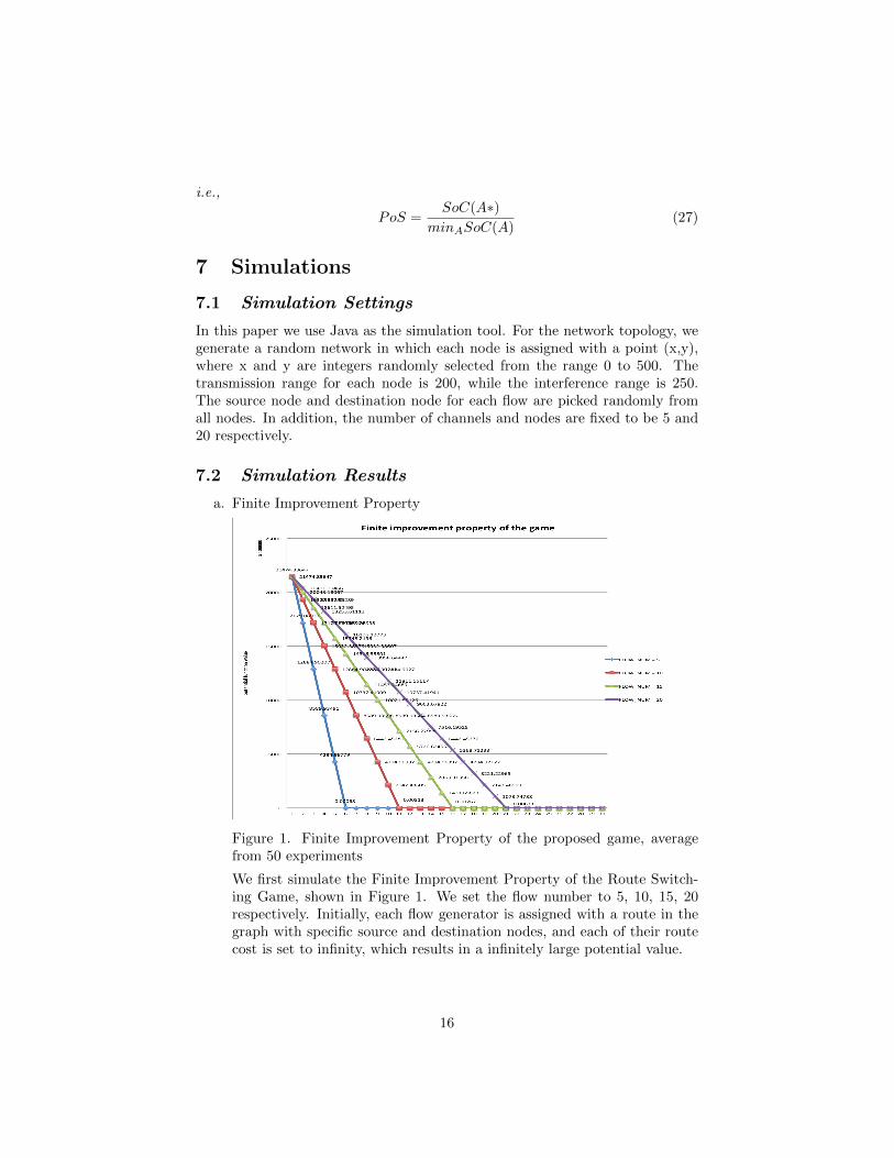
Figure 1. Finite Improvement Property of the proposed game, averagefrom 50 experiments

We first simulate the Finite Improvement Property of the Route Switch-ing Game, shown in Figure 1. We set the flow number to 5, 10, 15, 20respectively. Initially, each flow generator is assigned with a route in thegraph with specific source and destination nodes, and each of their routecost is set to infinity, which results in a infinitely large potential value.

16

After each improvement step, with each flow generator updating its routesaccording to the learning strategy, the potential value is gradually reduced,and eventually converges to a small value close to zero. Although the gamewith more flows converge more slowly, the Nash Equilibrium can still bereached quickly (around 21 iterations for 20 flows).

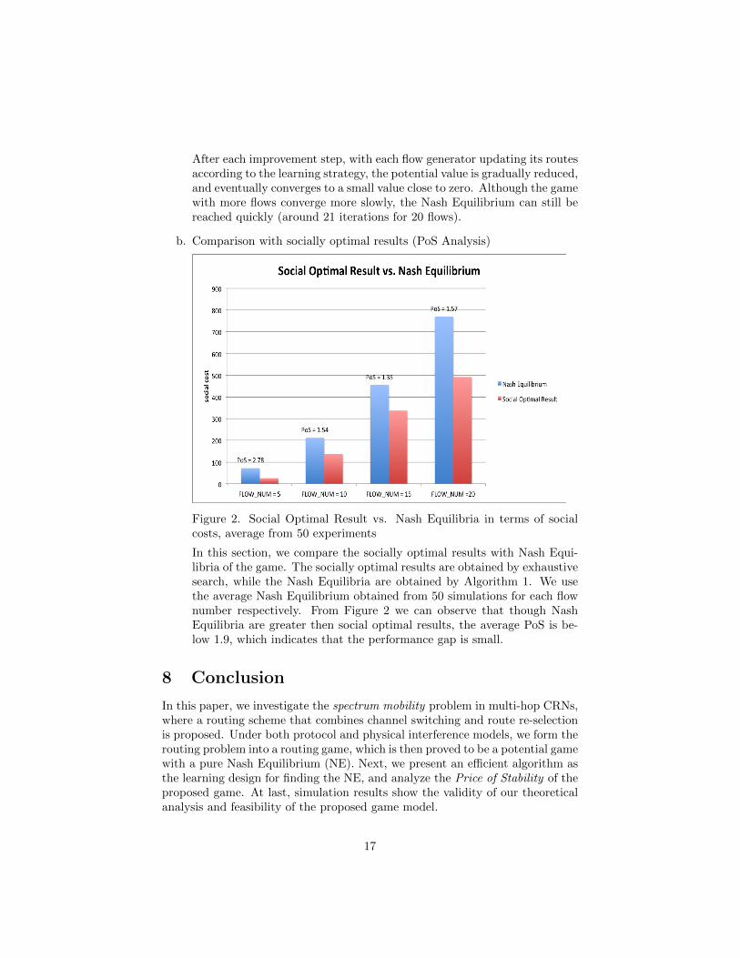
b. Comparison with socially optimal results (PoS Analysis)

Figure 2. Social Optimal Result vs. Nash Equilibria in terms of socialcosts, average from 50 experiments

In this section, we compare the socially optimal results with Nash Equi-libria of the game. The socially optimal results are obtained by exhaustivesearch, while the Nash Equilibria are obtained by Algorithm 1. We usethe average Nash Equilibrium obtained from 50 simulations for each flownumber respectively. From Figure 2 we can observe that though NashEquilibria are greater then social optimal results, the average PoS is be-low 1.9, which indicates that the performance gap is small.

8 Conclusion

In this paper, we investigate the spectrum mobility problem in multi-hop CRNs,where a routing scheme that combines channel switching and route re-selectionis proposed. Under both protocol and physical interference models, we form therouting problem into a routing game, which is then proved to be a potential gamewith a pure Nash Equilibrium (NE). Next, we present an efficient algorithm asthe learning design for finding the NE, and analyze the Price of Stability of theproposed game. At last, simulation results show the validity of our theoreticalanalysis and feasibility of the proposed game model.

17

References

[1] Qingkai Liang, Xinbing Wang, Xiaohua Tian, Fan Wu, Qian Zhang, Two-Dimensional Route Switching in Cognitive Radio Networks: A Game-Theoretical Framework. IEEE/ACM Transactions on Networking, 2014.

[2] Qinghai Xiao, Yunzhou Li, Ming Zhao, Shidong Zhou, Jing Wang, Oppor-tunistic channel selection approach under collision probability constraint incognitive radio systems. Computer Communications Volume 32, Issue 18,Pages 1903-2012 (15 December 2009).

[3] J.Zhao, G.Cao, Robust Topology Control in Multi-hop Cognitive Radio Net-works. Proceedings of IEEE INFOCOM, 2012

[4] M. Caleffi, I.F.Akyildiz, L.Paura, OPERA: Optimal Routing Metric forCognitive Radio Ad Hoc Networks. IEEE Transactions on Wireless Com-munications, vol.11, no.8, August 2012

[5] Tim Roughgarden, Noam Nisan, Eva Tardos, Vijay V. Vazirani, Algorith-mic Game Theory. Cambridge University Press 2007

[6] Ragavendran Gopalakrishnan, Jason R. Marden, Adam Wierman, An Ar-chitectural View of Game Theoretic Control. Newsletter ACM SIGMET-RICS Performance Evaluation Review archive, Volume 38 Issue 3, Decem-ber 2010, Pages 31-36

[7] Jonathan Levin Learning in Gamesl. Stanford, May 2006

18