Embed Size (px)
Citation preview
1
Channel Estimation for OpportunisticSpectrum Access: Uniform and Random
SensingQuanquan Liang, Mingyan Liu, Senior Member, IEEE, Dongfeng Yuan, Senior Member, IEEE
Abstract—The knowledge of channel statistics can be very helpful in making sound opportunistic spectrum access decisions.It is therefore desirable to be able to efficiently and accurately estimate channel statistics. In this paper we study the problemof optimally placing sensing/sampling times over a time window so as to get the best estimate on the parameters of an on-off renewal channel. We are particularly interested in a sparse sensing regime with a small number of samples relative tothe time window size. Using Fisher information as a measure, we analytically derive the best and worst sensing sequencesunder a sparsity condition. We also present a way to derive the best/worst sequences without this condition using a dynamicprogramming approach. In both cases the worst turns out to be the uniform sensing sequence, where sensing times are evenlyspaced within the window. Interestingly the best sequence is also uniform but with a much smaller sensing interval that requiresa priori knowledge of the channel parameters. With these results we argue that without a priori knowledge, a robust sensingstrategy should be a randomized strategy. We then compare different random schemes using a family of distributions generatedby the circular β ensemble, and propose an adaptive sensing scheme to effectively track time-varying channel parameters. Wefurther discuss the applicability of compressive sensing for this problem.
Index Terms—Spectrum sensing, channel estimation, Fisher information, random sensing, sparse sensing, uniform sensing.
✦
1 INTRODUCTION
R ECENT advances in software defined radio andcognitive radio [1] have given wireless devices
greater ability and opportunity to dynamically accessspectrum, thereby potentially significantly improvingspectrum efficiency and user performance [2], [3]. Akey enabling ingredient is thus high quality chan-nel sensing that allows the user to obtain accuratereal-time information on the condition of wirelesschannels. Spectrum sensing is often studied in twocontexts: at the physical layer and at the MAC layer.Physical layer spectrum sensing typically focuses onthe detection of instantaneous primary user signals.Examples like matched filter detection, energy detec-tion and feature detection have been proposed forcognitive radios [4]. MAC layer spectrum sensing [5],[6] is more of a resource allocation issue, where weare concerned with the scheduling problem of when tosense the channel and the estimation problem of ex-tracting statistical properties of the random variationin the channel.
• Q. Liang and M. Liu are with the Department of Electrical Engineeringand Computer Science, University of Michigan, Ann Arbor, MI 48109-2122, [email protected], [email protected]. Q. Liang is alsoaffiliated with the School of Information Science and Engineering,Shangdong University, Shangdong, China. D. Yuan is with the Schoolof Information Science and Engineering, Shangdong University.
• An earlier version of this paper appeared at the Information Theoryand Application Workshop (ITA), UC San Diego, CA, February 2010.This work is partially supported by NSF grant CCF 0910765 and NSFof China grant 60832008, 61071122.
In this paper we focus on the scheduling of channelsensing and study the effect different scheduling algo-rithms have on the accuracy of the resulting estimatewe obtain on channel parameters. In particular, we areinterested in a sparse sensing/sampling regime wherewe can use only a limited number of measurementsover a given period of time. The goal is to decidehow these limited number of measurements shouldbe scheduled so as to minimize the estimation er-ror within the maximum likelihood (ML) estimatorframework. Throughout the paper the terms sensingand sampling will be used interchangeably.
MAC layer channel estimation has been studied inrecent years. Below we review those most relevant tothe present paper. In [5] an ML estimator was intro-duced for renewal channels using a uniform samplingscheme. A more accurate but much more computa-tionally costly Bayesian estimator was introduced in[7], again based on uniform sensing. [8] analyzed therelationship between estimation accuracy, number ofsamples taken and the channel state transition prob-abilities by using the framework of [5]. [9] proposeda Hidden Markov Model (HMM) based channel sta-tus predictor using reinforcement learning techniques.[10] presented a channel estimation technique basedon wavelet transform followed by filtering.
In most of the above cited work, the focus is on theestimation problem given (sufficiently dense) uniformsampling of the channel, i.e., with equal time periodsbetween successive samples. This scheme will be re-ferred to as uniform sensing in the remainder of this
2
paper. We observe that due to constraints on time,energy, memory and other resources, a user may wishto perform channel sensing at much lower frequencieswhile still hoping for good estimates. This could berelevant for instance in cases where a user wants totrack the channel condition in between active datacommunication, or where a user needs to track alarge number of different channels. It is this sparsesampling scenario that we will focus on in this study,and the goal is to judiciously schedule these limitednumber of samples.
Our main contributions are summarized as follows.
• We demonstrate that when sampling is donesparsely, random sensing significantly outperformsuniform sensing.
• In the special case of exponentially distributedon/off durations, we obtain the best and worstpossible sampling schemes measured by theFisher information. We show that uniform sens-ing is the worst; any deviation from it improvesthe estimation accuracy. Interestingly, the bestsensing sequence is also uniform, but with amuch smaller sampling interval that requires theknowledge of the underlying channel parameter,thus unimplementable.
• We present an adaptive random sensing scheme thatcan very effectively track time-varying channelparameters, and is shown to outperform its coun-terpart using uniform sensing.
The remainder of this paper is organized as follows:Section 2 presents the channel models and Section 3gives the detail of the ML estimator. In Section 4 wepresent how the sampling scheme affects the estima-tion performance. In Section 5 we use the circularβ ensemble to examine different random samplingschemes. Section 6 presents an adaptive random sens-ing scheme, and Section 7 concludes the paper.
2 THE CHANNEL MODEL
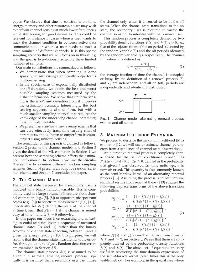
The channel state perceived by a secondary user ismodeled as a binary random variable. This is com-monly used in a large volume of literature, from chan-nel estimation (e.g., [5], [8]) to opportunistic spectrumaccess (e.g., [6]) to spectrum measurement (e.g., [11]).Specifically, let Z(t) denote the state of the channelat time t, such that Z(t) = 1 if the channel is sensedbusy at time t, and Z(t) = 0 otherwise.
In this paper our focus is on extracting and estimat-ing essential statistics given a sequence of measuredchannel states (0s and 1s) rather than the binarydetection of channel state (deciding between 0 and 1given the energy reading). For this purpose, we willassume that the channel state measurements are error-free throughout our analysis. Random detection errorsare examined in Section 5.5.
The channel state process Z(t) is assumed to bea continuous-time alternating renewal process. Typ-ically, it is assumed that a secondary user can utilize
the channel only when it is sensed to be in the offstates. When the channel state transitions to the onstate, the secondary user is required to vacate thechannel so as not to interfere with the primary user.
This random process is completely defined by twoprobability density functions f1(t) and f0(t), t > 0, i.e.,that of the sojourn times of the on periods (denoted bythe random variable T1) and the off periods (denotedby the random variable T0), respectively. The channelutilization u is defined as
u =E[T1]
E[T1] + E[T0], (1)
the average fraction of time the channel is occupiedor busy. By the definition of a renewal process, T1
and T0 are independent and all on (off) periods areindependently and identically distributed.
Fig. 1. Channel model: alternating renewal processwith on and off states
3 MAXIMUM LIKELIHOOD ESTIMATION
We proceed to describe the maximum likelihood (ML)estimator [12] we will use to estimate channel param-eters from a sequence of channel state observations.
An alternative renewal process is completely char-acterized by the set of conditional probabilitiesPij(∆t), i, j ∈ {0, 1}, ∆t ≥ 0, defined as the probabilitythat given i was observed ∆t time units ago, j isnow observed. This quantity is also commonly knownas the semi-Markov kernel of an alternating renewalprocess [13]. Assuming the process is in equilibrium,standard results from renewal theory [13] suggest thefollowing Laplace transforms of the above transitionprobabilities:
P ∗00(s) =
1
s− {1 − f∗
1 (s)} {1 − f∗0 (s)}
E[T0]s2 {1 − f∗1 (s)f∗
0 (s)} ,
P ∗01(s) =
{1 − f∗1 (s)} {1 − f∗
0 (s)}E[T0]s2 {1 − f∗
1 (s)f∗0 (s)} ,
P ∗10(s) =
{1 − f∗1 (s)} {1 − f∗
0 (s)}E[T1]s2 {1 − f∗
1 (s)f∗0 (s)} ,
P ∗11(s) =
1
s− {1 − f∗
1 (s)} {1 − f∗0 (s)}
E[T1]s2 {1 − f∗1 (s)f∗
0 (s)} ,
(2)
where f∗1 (s) and f∗
0 (s) are the Laplace transforms off1(t) and f0(t), respectively. We see that these are com-pletely defined by the probability density functionsf1(t) and f0(t). The above set of equations are veryuseful in recovering the time-domain expressions ofthe semi-Markov kernel (often times this is the onlyviable method). For example, in the special case where
3
the channel has exponentially distributed on/off pe-riods, we have
{
f1(t) = θ1e−θ1t
f0(t) = θ0e−θ0t .
(3)
Their corresponding Laplace transforms and expecta-tions are{
f∗1 (s) = θ1/(s + θ1)
f∗0 (s) = θ0/(s + θ0) ,
{
E[T1] = 1/θ1
E[T0] = 1/θ0 .
Substituting the above expressions into (2) followedby an inverse Laplace transform we get the statetransition probability as follows:
Pij(∆t) = uj(1−u)1−j+(−1)j+iu1−i(1−u)ie−(θ0+θ1)∆t ,(4)
where u = E[T1]E[T1]+E[T0]
, as defined earlier.The relevant estimation problem is stated as fol-
lows. Assume that the on/off periods are given bycertain known distribution functions f0(t) and f1(t)but with unknown parameters. Suppose we obtainm samples [z1, z2, · · · , zm], taken at sampling times[t1, t2, · · · , tm], respectively. We wish to use these sam-ples to estimate the unknown parameters.
First note that the channel utilization factor u canbe estimated through the sample mean of the mmeasurements as follows
u =1
m
m∑
i=1
zi . (5)
Let θ be the unknown parameters of the on/offdistributions: θ = [θ1, θ0]. Note that in general θ1
and θ0 are vectors themselves. Then the likelihoodfunction is given by
L(θ) = Pr{Z; θ}= Pr{Ztm = zm, Ztm−1
= zm−1,
Ztm−2= zm−2, . . . , Zt1 = z1; θ} . (6)
The idea of ML estimation is to find the value ofθ that maximizes the log likelihood function lnL(θ).This method has been used extensively in the lit-erature [14]–[18]. For a fixed set of data and un-derlying probability model, the ML estimator se-lects the parameter value that makes the data “mostlikely” among all possible choices. Under certain(fairly weak) regularity conditions the ML estimatoris asymptotically optimal [19].
The question we wish to investigate is what im-pact the selection of the sampling time sequence[t1, t2, · · · , tm] has on the performance of this estima-tor, given a limited number of samples m. For theremainder of our analysis we will limit our attentionto the case where the channel on/off durations aregiven by exponential distributions. This is for bothmathematical tractability and simplicity of presenta-tion. Other distributions are explored in our numericalexperiments. It’s worth noting that the exponentialdistribution assumption is adopted widely in channel
models [5]–[7]; spectrum measurement studies havealso found it to be a good approximation of realchannel vacancy durations [11], [20].
Since the exponential distribution is defined by asingle parameter, we have now θ = [θ1, θ0], where θ1
and θ0 are the two unknown scalar parameters of theon and off exponential distributions, respectively. Us-ing the memoryless property, the likelihood functionis given by (7) where ∆ti = ti−ti−1. The first quantityon the right is taken to be
Pr{zt1 = z1; θ} = uz1(1 − u)1−z1 , (8)
the steady state probability of finding the channel ina particular state. This is justified by assuming thatthe channel is in equilibrium.
The second quantity Pzi−1zi(∆ti; θ) is given in Eqn(4). Combining these two quantities, we have
L(θ0, θ1) = L(θ)
= uz1(1 − u)1−z1
m∏
i=2
(
uzi(1 − u)1−zi
+ (−1)zi+zi−1u1−zi−1(1 − u)zi−1e−(θ0+θ1)∆ti)
.(9)
The estimates for the parameters are found by solving
(θ1, θ0) = arg maxθ1,θ0
lnL(θ0, θ1) . (10)
The above joint optimization proves to be computa-tionally complex and analytically intractable. Instead,we adopt the following sub-optimal estimation pro-cedure, also used in [5]. We first estimate u using Eqn
(5), and take θ1 = (1−u)θ0
u . Due to the exponentialassumption, it can be shown that this estimate ofu is unbiased regardless of the sequence [t1, · · · , tm]as long as it is determined offline. The likelihoodfunction (9) can then be re-written as
L(θ0) = uz1(1 − u)1−z1
m∏
i=2
(
uzi(1 − u)1−zi
+(−1)zi+zi−1u1−zi−1(1 − u)zi−1e−θ0∆ti/u)
. (11)
The estimation of θ0 is then derived by solvingmaxθ0
lnL(θ0)In our analysis, we will use this procedure by
treating u as a known constant and solely focus onthe estimation of θ0, with the understanding that uis separately and unbiasedly estimated, and once wehave the estimate for θ0 we have the estimate for θ1.It has to be noted that this procedure is in generalnot equivalent to solving (10). However, this is areasonable approach, computationally feasible, andmuch more amenable to analysis.
4 BEST AND WORST SENSING SEQUENCES
The goal of this study is to judiciously schedule avery limited number of sampling times so that theestimation accuracy is least affected. We first argueintuitively why the commonly used uniform sampling
4
L(θ) = Pr{Z; θ} = Pr{Zt1 = z1; θ}m∏
i=2
Pr{Zti = zi|Zti−1= zi−1; θ} = Pr{Zt1 = z1; θ}
m∏
i=2
Pzi−1zi(∆ti; θ) . (7)
does not perform well when the number of samplesallowed is limited. We then present a precise analysisthrough the use of Fisher information in the caseof exponential on/off distributions. We show thatusing this measure, under a certain sparsity conditionuniform sensing is the worst schedule in terms ofestimation accuracy. We also derive an upper boundon the Fisher information as well as the samplingsequence achieving this upper bound. These provideus with useful benchmarks to assess any arbitrarysampling sequence.
4.1 An intuitive explanation
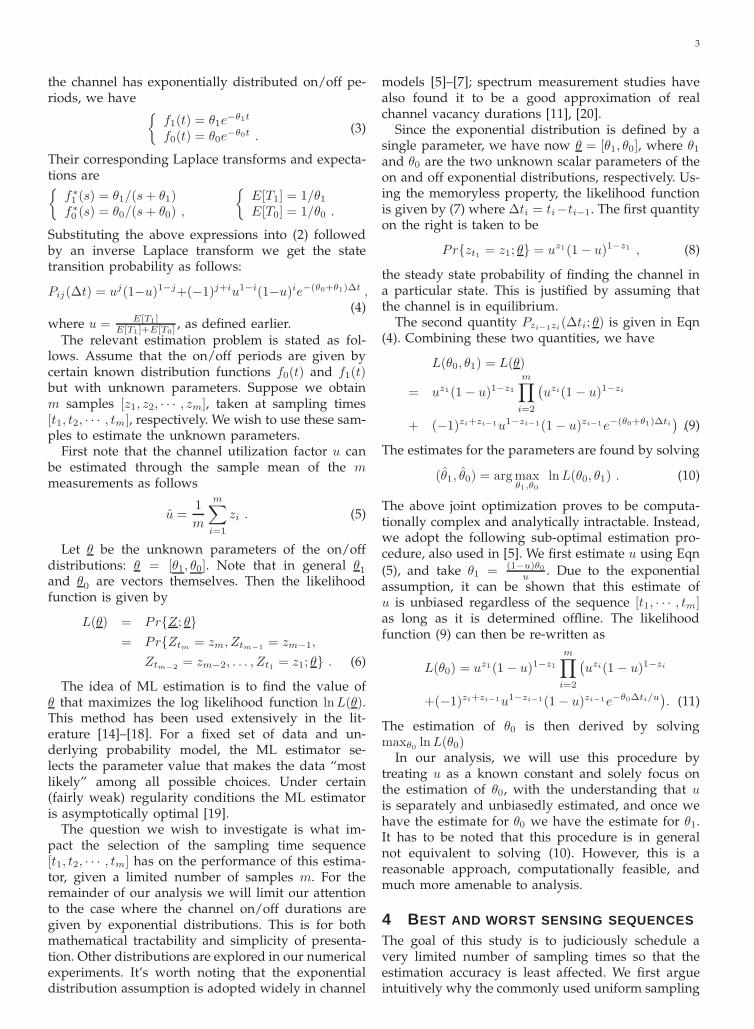
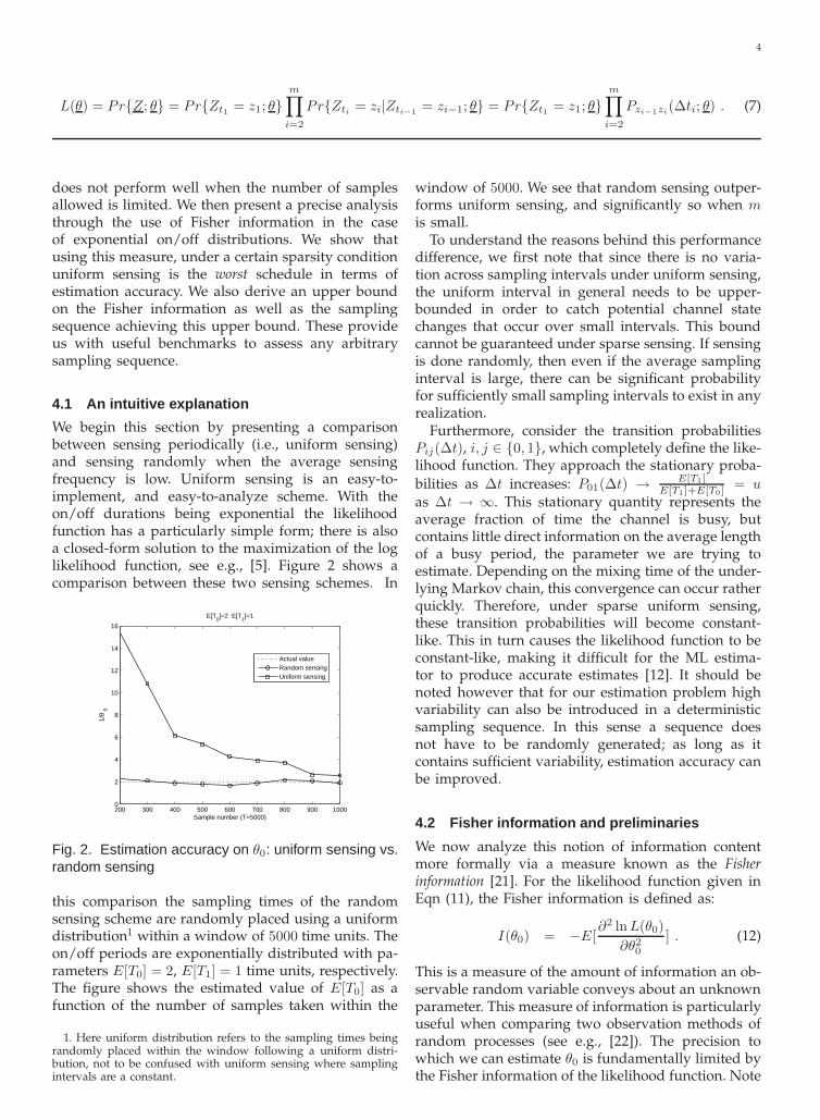
We begin this section by presenting a comparisonbetween sensing periodically (i.e., uniform sensing)and sensing randomly when the average sensingfrequency is low. Uniform sensing is an easy-to-implement, and easy-to-analyze scheme. With theon/off durations being exponential the likelihoodfunction has a particularly simple form; there is alsoa closed-form solution to the maximization of the loglikelihood function, see e.g., [5]. Figure 2 shows acomparison between these two sensing schemes. In
200 300 400 500 600 700 800 900 10000
2
4
6
8
10
12
14
16
Sample number (T=5000)
1/θ
0
E[T0]=2 E[T
1]=1
Actual valueRandom sensingUniform sensing
Fig. 2. Estimation accuracy on θ0: uniform sensing vs.random sensing
this comparison the sampling times of the randomsensing scheme are randomly placed using a uniformdistribution1 within a window of 5000 time units. Theon/off periods are exponentially distributed with pa-rameters E[T0] = 2, E[T1] = 1 time units, respectively.The figure shows the estimated value of E[T0] as afunction of the number of samples taken within the
1. Here uniform distribution refers to the sampling times beingrandomly placed within the window following a uniform distri-bution, not to be confused with uniform sensing where samplingintervals are a constant.
window of 5000. We see that random sensing outper-forms uniform sensing, and significantly so when mis small.
To understand the reasons behind this performancedifference, we first note that since there is no varia-tion across sampling intervals under uniform sensing,the uniform interval in general needs to be upper-bounded in order to catch potential channel statechanges that occur over small intervals. This boundcannot be guaranteed under sparse sensing. If sensingis done randomly, then even if the average samplinginterval is large, there can be significant probabilityfor sufficiently small sampling intervals to exist in anyrealization.
Furthermore, consider the transition probabilitiesPij(∆t), i, j ∈ {0, 1}, which completely define the like-lihood function. They approach the stationary proba-
bilities as ∆t increases: P01(∆t) → E[T1]E[T1]+E[T0]
= u
as ∆t → ∞. This stationary quantity represents theaverage fraction of time the channel is busy, butcontains little direct information on the average lengthof a busy period, the parameter we are trying toestimate. Depending on the mixing time of the under-lying Markov chain, this convergence can occur ratherquickly. Therefore, under sparse uniform sensing,these transition probabilities will become constant-like. This in turn causes the likelihood function to beconstant-like, making it difficult for the ML estima-tor to produce accurate estimates [12]. It should benoted however that for our estimation problem highvariability can also be introduced in a deterministicsampling sequence. In this sense a sequence doesnot have to be randomly generated; as long as itcontains sufficient variability, estimation accuracy canbe improved.
4.2 Fisher information and preliminaries
We now analyze this notion of information contentmore formally via a measure known as the Fisherinformation [21]. For the likelihood function given inEqn (11), the Fisher information is defined as:
I(θ0) = −E[∂2 lnL(θ0)
∂θ20
] . (12)
This is a measure of the amount of information an ob-servable random variable conveys about an unknownparameter. This measure of information is particularlyuseful when comparing two observation methods ofrandom processes (see e.g., [22]). The precision towhich we can estimate θ0 is fundamentally limited bythe Fisher information of the likelihood function. Note
5
that in (12) we have suppressed u from the argumentas u is estimated separately and taken as a constantin our subsequent analysis.
Due to the product form of the likelihood function,we have
I(θ0) = −E[
m∑
i=2
∂2 ln[αi + βie−θ0∆ti/u]
∂θ20
]
=
m∑
i=2
∆t2iu2
E[ −αiβie
−θ0∆ti/u
(αi + βie−θ0∆ti/u)2]
, (13)
where αi = uzi(1 − u)1−zi and βi =(−1)zi+zi−1u1−zi−1(1 − u)zi−1 . Define:
g(θ0; ∆ti) =∆t2iu2
E[ −αiβie
−θ0∆ti/u
(αi + βie−θ0∆ti/u)2]
, (14)
so that the Fisher information can be simply writtenas I(θ0) =
∑mi=2 g(θ0; ∆ti). The function g() will be re-
ferred to as the Fisher function in our discussion. Notethat g() is a function of both ∆ti and θ0. However,we will suppress θ0 from the argument and write itsimply as g(∆t). This is because our analysis focuseson how this function behaves as we select different∆t (the sampling interval) while holding θ0 constant.Note that the first term in Eqn (11) does not appearin the above expression. This is because this firstterm is only a function of u (see Eqn (8)), which isseparately estimated using Eqn (5) and not viewed asa function of θ0. Therefore the term disappears afterthe differentiation.
The expectation on the RHS of (13) can be calcu-lated by considering all four possibilities for the pair(zi−1, zi), i.e., (0, 0), (0, 1), (1, 0), and (1, 1). Using Eqn(4), we obtain the transition probability of each caseto be (1 − u)P00(∆t), (1 − u)P01(∆t), uP10(∆t) anduP11(∆t), respectively. We can therefore calculate theFisher function as in Eqn (15). Below we show that un-der a certain sparsity condition on the sampling rate,the Fisher function is strictly convex and the Fisherinformation is minimized under uniform sampling.
Condition 1: (Sparsity condition) Let α = max{2 +√2, ln(1−u
u ), ln( u1−u )}. This condition requires that
∆t > αu/θ0.Lemma 1: The Fisher function g(∆t) given in Eqn
(15) is strictly convex under Condition 1.The proof of this lemma can be found in the Ap-
pendix. Using this lemma we next derive tight lowerand upper bounds of the Fisher information.
4.3 A tight lower bound on the Fisher information
Lemma 2: For any n ∈ N, n ≥ 1, T ∈ R, T > (n +1)αu/θ0, and αu/θ0 < ∆t < T − nαu/θ0, the functionG(∆t) = ng(T−∆t
n ) + g(∆t) has a minimum of (n +1)g( T
n+1 ) attained at ∆t = Tn+1 .
Proof: Setting the first derivative of G to zeroand solving for ∆t results in solving the equationg
′
(∆t) = g′
(T−∆tn ). Since the arguments on both
side satisfy Condition 1, by the assumption of thelemma, g is strictly convex according to Lemma 1and g
′
is a strictly monotonic function. Thereforethere exists a unique solution within the range of(αu/θ0, T − nαu/θ0) to this equation at ∆t = T
n+1 .Next we calculate the second derivative of G at this
point. Since G′′
(∆t) = g′′
(∆t) + 1ng
′′
(T−∆tn ), we have
G′′
( Tn+1 ) = (1+ 1
n )g′′
( Tn+1 ). Since T > (n+1)αu/θ0, g is
convex at this stationary point by Lemma 1. Hence Gis convex at this point and it is thus a global minimumwithin the range (αu/θ0, T − nαu/θ0); the minimumvalue is (n + 1)g( T
n+1 ), completing the proof.Theorem 1: Consider a period of time [0, T ], in
which we wish to schedule m ≥ 3 sampling points,including one at time 0 and one at time T . Denote thesequence of time spacings between these samples as∆t = [∆t2, ∆t3, · · · , ∆tm], where
∑mi=2 ∆ti = T . For a
given sequence ∆t, define the Fisher information I(θ0)as in Eqn (13) and rewrite it as I(θ0; ∆t) to emphasizeits dependence on ∆t. Assuming T > (m − 1)αu/θ0,then we have
min∆t∈Am
I(θ0; ∆t) = (m − 1)g(T
m − 1),
where Am = {∆ti :∑m
i=2 ∆ti = T, ∆ti > αu/θ0, i =2, · · · , m}, and with the minimum achieved at ∆ti =
Tm−1 , i = 2, · · · , m.
Proof: We prove this by induction on m.Induction basis: For m = 3,
I(θ0; ∆t) = g(∆t2) + g(∆t3).
Using Lemma 1 in the special case of n = 1 the resultfollows.
Induction step: Suppose the result holds for3, 4, . . .m, we want to show it also holds for m + 1for T > mαu/θ0. Note that in this case ∆t ∈ Am+1
implies that αu/θ0 < ∆tm+1 < T − (m − 1)αu/θ0,which will be denoted as ∆tm+1 ∈ Am+1 below forconvenience. We thus have
min∆t∈Am+1
{I(θ0; ∆t)}
= min∆t∈Am+1
{
m∑
i=2
g(∆ti) + g(∆tm+1)
}
= min∆tm+1∈Am+1
{
min∑
∆ti=T−∆tm+1
{
m∑
i=2
g(∆ti)
}
+g(∆tm+1)
}
= min∆tm+1∈Am+1
{
(m − 1)g(T − ∆tm+1
m − 1)
+g(∆tm+1)
}
= mg(T
m) ,
where the third equality is due to the induction hy-pothesis and the first term on the RHS is obtained
6
g(∆t) =∆t2
u2e−θ0∆t/u
[ u2(1 − u)
u − ue−θ0∆t/u+
u(1 − u)2
(1 − u) − (1 − u)e−θ0∆t/u− u(1 − u)2
(1 − u) + ue−θ0∆t/u− u2(1 − u)
u + (1 − u)e−θ0∆t/u
]
.
(15)
at ∆ti = T−∆tm+1
m−1 , i = 2, . . . , m. The last equalityinvokes Lemma 2 in the special case of n = m − 1,and is obtained at ∆tm+1 = T
m . Combining these weconclude that the minimum value of Fisher informa-tion is mg( T
m ), when ∆ti = Tm , i = 2, . . . , m + 1. Thus
the case m + 1 also holds, completing the proof.Theorem 1 states that given the total sensing period
T and the total number of samples m, providedthat the sampling is done sparsely (per Condition1), the Fisher information attains its minimum whenall sampling intervals are the same, i.e a uniformsensing schedule. In this sense uniform sensing isthe worst possible sensing scheme; any deviation fromit, while keeping the same average sampling intervalT/(m − 1), can only increase the Fisher information.As we have seen in Figure 2, this increase in Fisherinformation becomes more significant when samplinggets sparser, i.e., when m decreases.
4.4 A tight upper bound on the Fisher information
The derivation of the upper bound follows very sim-ilar steps as those for the lower bound.
Lemma 3: For any T ∈ R, T > 2αu/θ0, and αu/θ0 <∆t < T − αu/θ0, the function F (∆t) = g(T − ∆t) +g(∆t) has a maximum of g(αu/θ0) + g(T − αu/θ0)attained at ∆t = αu/θ0 or ∆t = T − αu/θ0.
Proof: We first prove that F is convex under thestated conditions. We have F
′
(∆t) = g′
(∆t) − g′
(T −∆t). Since g is strictly convex under the stated condi-tions, by Lemma 1 g
′
is monotonic increasing. ThusF
′
is also monotonic increasing, hence F is convex. Itfollows that the maximum of F (∆t) is attained at oneand/or the other extreme point of ∆t. In either casewe have
F (αu/θ0) = F (T −αu/θ0) = g(αu/θ0)+ g(T −αu/θ0).
Theorem 2: Consider a period of time [0, T ], inwhich we wish to schedule m ≥ 3 sampling points,including one at time 0 and one at time T . Denotethe sequence of time spacings between these samplesas ∆t = [∆t2, ∆t3, · · · , ∆tm], where
∑mi=2 ∆ti = T .
Assuming T > (m − 1)αu/θ0, then we have
max∆t∈Am
I(θ0; ∆t) = (m − 2)g(αu/θ0)
+g(T − (m − 2)αu/θ0),
where Am = {∆ti :∑m
i=2 ∆ti = T, ∆ti > αu/θ0, i =2, · · · , m}, and with the maximum achieved at ∆ti =αu/θ0, i = 2, · · · , m− 1 and ∆tm = T − (m− 2)αu/θ0.
Proof: We prove this by induction on m.
Induction basis: For m = 3, I(θ0; ∆t) = g(∆t2) +g(∆t3). Using Lemma 3 the result immediately fol-lows.
Induction step: Suppose the result holds for3, 4, . . .m, we want to show it also holds for m+1 forT > mαu/θ0. Again in this case ∆t ∈ Am+1 impliesthat αu/θ0 < ∆tm+1 < T−(m−1)αu/θ0, which will bedenoted as ∆tm+1 ∈ Am+1 for convenience. We thushave
max∆t∈Am+1
{I(θ0; ∆t)}
= max∆t∈Am+1
{
m∑
i=2
g(∆ti) + g(∆tm+1)
}
= max∆tm+1∈Am+1
{
max∑
∆ti=T−∆tm+1
{
m∑
i=2
g(∆ti)
}
+g(∆tm+1)
}
= max∆tm+1∈Am+1
{
(m − 2)g(αu/θ0)
+g(T − ∆tm+1 − (m − 2)αu/θ0) + g(∆tm+1)
}
= (m − 1)g(αu/θ0) + g(T − (m − 1)αu/θ0) ,
where the third equality is due to the induction hy-pothesis and the first term on the RHS is obtained at∆ti = αu/θ0, i = 2, . . . , m−1 and ∆tm = T −∆tm+1−(m − 2)αu/θ0. The last equality invokes Lemma 3,and is obtained at ∆tm+1 = T − (m − 1)αu/θ0 or∆tm+1 = αu/θ0. Thus the case m + 1 also holds,completing the proof.
We see from this theorem that under the sparsitycondition, the best sensing sequence is to sample atthe smallest interval that the condition would allow,till we use all the m−2 samples we have the freedomof placing. This produces a pseudo uniform sequence ofsampling times; it forms a uniform sequence exceptfor the last sampling interval. It can be shown thatif we remove the constraint of having a windowof T , but rather seek to optimally place m pointssubject to the sparsity condition, then the optimalsequence would be exactly uniform with the interval∆ti = αu/θ0. However, it should be emphasized thatsince θ0 is the very thing we are trying to estimate,it would be unreasonable to suggest that this optimalinterval is known a priori. Thus this optimal sequenceis not implementable. It nevertheless sheds light onthe nature of the sequence that maximizes the Fisherinformation.
7
4.5 Best and worst sampling schemes without thesparsity condition
We next show how to obtain the best and worst sens-ing sequences in a more general setting, without therequirement of Condition 1, via the use of dynamicprogramming. While this result is more general com-pared to those derived under the sparsity condition,structurally they are not as easy to identify and arethus given in a numerical form. We also note thatthese sequences are not practically implementable asthey assume a priori knowledge of the parametersto be estimated. They are derived only to serve asbenchmarks.
Denote by π a sampling policy given by the timesequence [t1, t1, · · · , tm]. Then the optimal samplingpolicy is given by
π∗ = arg maxπ∈Π
I(θ0) , (16)
where the set of admissible policies Π = {ti : t1 =0, tm = T, 0 < t2 < · · · < tm−1 < T }.
The maximum I(θ0) can be recursively solvedthrough the set of dynamic programming equationsgiven below:
V (1, t) = g(T − t), ∀ 0 ≤ t < T ;
V (k, t) = maxt<x<T
[g(x − t) + V (k − 1, x)],
∀ 0 ≤ t < T, k = 2, 3, · · · , m − 1 ,(17)
and
max I(θ0) = max0<t<T
[g(t) + V (m − 1, t)] . (18)
Here the value function V (k, t) denotes the maximumachievable Fisher information given we last sampledat time t, with k points remaining to be placed be-tween (t, T ].
Note that since t is continuous, the pair (k, t) hasan uncountable state space. In computing the DPequation (17) we discretize t and T into small stepsand require that both be integer multiples of this smallquantity. The resulting DP has a finite state space andis solved backwards in time [23].
It is straightforward to see the exact same pro-cedure can be used to find the sampling sequencethat minimizes the Fisher information, thus giving theworst sampling sequence. It turns out that the worstsampling sequence in this case coincides with theworst sequence derived under the sparsity condition,i.e., it is also the uniform sequence.
4.6 A comparison
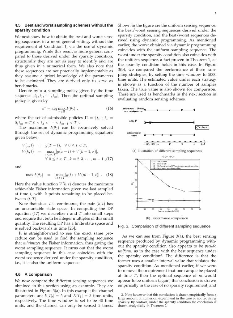
We now compare the different sensing sequences weobtained in this section using an example. They areillustrated in Figure 3(a). In this example the channelparameters are E[T0] = 5 and E[T1] = 3 time units,respectively. The time window is set to be 40 timeunits, and the channel can only be sensed 5 times.
Shown in the figure are the uniform sensing sequence,the best/worst sensing sequences derived under thesparsity condition, and the best/worst sequences de-rived using dynamic programming. As mentionedearlier, the worst obtained via dynamic programmingcoincides with the uniform sampling sequence. Theworst under the sparsity condition also coincides withthe uniform sequence, a fact proven in Theorem 1, asthe sparsity condition holds in this case. In Figure3(b), we compared the performance of these sam-pling strategies, by setting the time window to 5000time units. The estimated value under each strategyis shown as a function of the number of samplestaken. The true value is also shown for comparison.These are used as benchmarks in the next section inevaluating random sensing schemes.
(a) Illustration of different sampling sequences
10 20 30 40 50 60 70 80 900
5
10
15
20
25
30
35
Sample number (T=5000)
1/θ 0
E[T0]=5 E[T
1]=3
Actual valueBest by DPUniform/worst by DP/worst under sparsity conditionBest under sparsity condition
(b) Performance comparison
Fig. 3. Comparison of different sampling sequence
As we can see from Figure 3(a), the best sensingsequence produced by dynamic programming with-out the sparsity condition also appears to be pseudouniform, as in the case with the best sequence underthe sparsity condition2. The difference is that theformer uses a smaller interval value that violates thesparsity condition. As mentioned earlier, if we wereto remove the requirement that one sample be placedat time T , then the optimal sequence of m wouldappear to be uniform (again, this conclusion is drawnempirically in the case of no sparsity requirement, and
2. Note however that this conclusion is drawn empirically from alarge amount of numerical experiment in the case of not requiringsparsity. By contrast, under the sparsity condition the conclusion isdrawn analytically in Theorem 2.
8
precisely and analytically in the case of sparsity), withthe optimal interval being the value that maximizes(15). Interestingly, the worst sequence is also uniformwith or without the sparsity condition.
What this result suggests is that in the ideal case ifwe have a priori knowledge of the channel parame-ters, to maximize the Fisher information the best thingto do is indeed to sense uniformly. The difficulty ofcourse is that without this knowledge we have no wayof deciding what the optimal interval should be, anduniform sensing would be a bad decision as it couldturn out to be the worst with an unfortunate choiceof the sampling interval.
In such cases, the robust thing to do is simply tosense randomly, so that with some probability we willhave sampling intervals close to the actual optimum.This is investigated in the next section.
5 RANDOM SENSING
Under a random sensing scheme, the sampling in-tervals ∆ti are generated according to some distri-bution f(∆t) (this may be done independently orjointly). Below we first analyze how the resultingFisher information is affected, and then use a familyof distributions generated by the circular β ensembleto examine the performance of different distributions.
5.1 Effect on the Fisher information
We begin by examining the expectation of the Fisherfunction, averaged over randomly generated sam-pling intervals, calculated as (19), where the Taylorexpansion is around the expected sampling intervalµo = E[∆t], or T/(m − 1) for given window T andm number of samples taken, and µn =
∫ ∞
0(∆t −
µo)nf(∆t)d∆t is the nth order central moment of ∆t.
In order to have a fair comparison we will assumeT and m are fixed, thus fixing the average samplinginterval µo under different sampling schemes. Alsonote that the value g(n)(µo) is completely determinedby the channel statistics and not the sampling se-quence. Consequently the expected value of the Fisherfunction is affected by the selection of a samplingscheme only through the higher order central mo-ments of the distribution f(). Note that the expecta-tion of the Fisher function under uniform samplingwith constant sampling interval µo is simply g(µo)(i.e., only the first term on the right hand side re-mains). Therefore any random scheme would improveupon this if it results in a positive sum over thehigher order terms. While the above equation doesnot immediately lead to an optimal selection of arandom scheme, it is possible to seek one from afamily of distribution functions through optimizationover common parameters.
Before we proceed with this in the next subsection,we compare the normal, uniform and exponentialrandom sampling schemes using the above analysis.
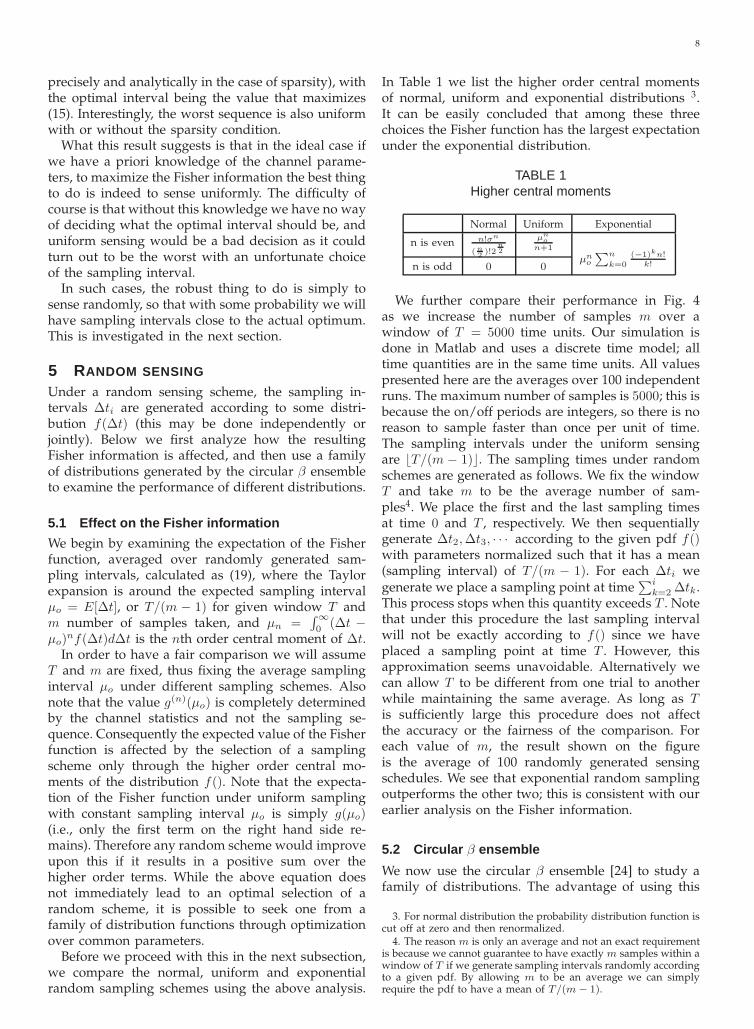
In Table 1 we list the higher order central momentsof normal, uniform and exponential distributions 3.It can be easily concluded that among these threechoices the Fisher function has the largest expectationunder the exponential distribution.
TABLE 1Higher central moments
Normal Uniform Exponential
n is even n!σn
( n2
)!2n2
µno
n+1
n is odd 0 0µn
o
∑n
k=0
(−1)kn!k!
We further compare their performance in Fig. 4as we increase the number of samples m over awindow of T = 5000 time units. Our simulation isdone in Matlab and uses a discrete time model; alltime quantities are in the same time units. All valuespresented here are the averages over 100 independentruns. The maximum number of samples is 5000; this isbecause the on/off periods are integers, so there is noreason to sample faster than once per unit of time.The sampling intervals under the uniform sensingare ⌊T/(m − 1)⌋. The sampling times under randomschemes are generated as follows. We fix the windowT and take m to be the average number of sam-ples4. We place the first and the last sampling timesat time 0 and T , respectively. We then sequentiallygenerate ∆t2, ∆t3, · · · according to the given pdf f()with parameters normalized such that it has a mean(sampling interval) of T/(m − 1). For each ∆ti wegenerate we place a sampling point at time
∑ik=2 ∆tk.
This process stops when this quantity exceeds T . Notethat under this procedure the last sampling intervalwill not be exactly according to f() since we haveplaced a sampling point at time T . However, thisapproximation seems unavoidable. Alternatively wecan allow T to be different from one trial to anotherwhile maintaining the same average. As long as Tis sufficiently large this procedure does not affectthe accuracy or the fairness of the comparison. Foreach value of m, the result shown on the figureis the average of 100 randomly generated sensingschedules. We see that exponential random samplingoutperforms the other two; this is consistent with ourearlier analysis on the Fisher information.
5.2 Circular β ensemble
We now use the circular β ensemble [24] to study afamily of distributions. The advantage of using this
3. For normal distribution the probability distribution function iscut off at zero and then renormalized.
4. The reason m is only an average and not an exact requirementis because we cannot guarantee to have exactly m samples within awindow of T if we generate sampling intervals randomly accordingto a given pdf. By allowing m to be an average we can simplyrequire the pdf to have a mean of T/(m − 1).
9
E[g(∆t)] =
∫ ∞
0
g(∆t)f(∆t)d∆t =
∫ ∞
0
[g(µo) + g′(µo)(∆t − µo) + · · · + g(n)(µo)(∆t − µo)n
n!+ · · · ]f(∆t)d∆t
= g(µo) + g′(µo)µ1 + · · · + g(n)(µo)µn
n!+ · · · (19)
20 40 60 80 100 120 140 160 1800
5
10
15
20
25
30
35
Average sample number (T=5000)
1/θ
0
E[T0]=2 E[T
1]=1
Actual valueNormalUniformExponentialUniform/worst by DP/worst under sparsity conditionBest under sparsity conditionBest by DP
Fig. 4. Performance comparison of random sensing
ensemble is that with a single tunable parameter wecan approximate a wide range of different distribu-tions while keeping the same average sampling rate.
The circular β ensemble may be viewed as givenby n eigenvalues, denoted as λj = eiφj , j = 1, · · · , n.These eigenvalues have a joint probability densityfunction proportional to the following:
∏
1≤k<l≤n
|eiφk − eiφl |β , −π < φj ≤ π, j, k, l = 1, · · · , n,
where β > 0 is a model parameter. In the specialcases β = 1, 2 and 4, this ensemble describes the jointprobability density of the eigenvalues of random or-thogonal, unitary and sympletic matrices, respectively[24].
We use the set of eigenvalues generated from theabove joint pdf to determine the placement of samplepoints in the interval [0, T ] in the following manner.In [25] a procedure is introduced to generate a setof values φj , j = 1, 2, · · · , n that follow the abovejoint pdf. Setting n = m, these n eigenvalues arethen placed along a unit circle (each at the positiongiven by φj), which are subsequently mapped ontothe line segment [0, 1]. Scaling this segment to [0, T ]gives us the m sampling times. The intervals betweenthese points now follow a certain joint distributionindexed by β. Below we will refer to this methodof generating sample points/intervals as using thecircular β ensemble.
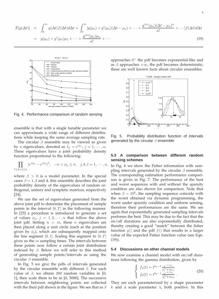
In Fig. 5 we give the pdfs of intervals generatedby the circular ensemble with different β. For eachvalue of β, we obtain 200 random variables in [0,1], then scale them to be in [0, 5000]. The successiveintervals between neighboring points are collectedwith the their pdf shown in the figure. We see that as β
approaches 0+ the pdf becomes exponential-like andas β approaches +∞, the pdf becomes deterministic;these are well known facts about circular ensembles.
0 50 100 150 200 250 3000
0.1
0.2
0.3
0.4
0.5
0.6
0.7
0.8
0.9
1
t
f(t)
T=5000 Sample number=200
0 20 400
0.05
0.1
0.15
β=10−6
β=1
β=2
β=4
β=106
Fig. 5. Probability distribution function of intervalsgenerated by the circular β ensemble
5.3 A comparison between different randomsensing schemes
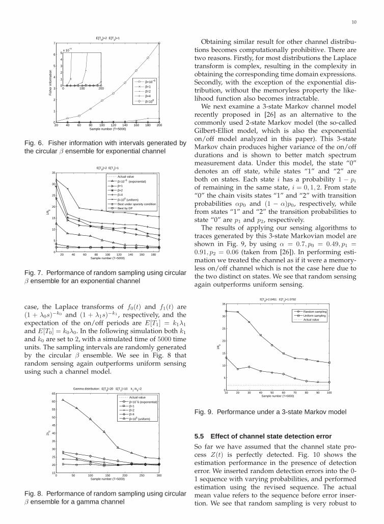
In Fig. 6 we show the Fisher information with sam-pling intervals generated by the circular β ensemble.The corresponding estimation performance compari-son is given in Fig. 7. The performance of the bestand worst sequences with and without the sparsitycondition are also shown for comparison. Note thatwhen β = 106, the sampling sequence coincide withthe worst obtained via dynamic programming, theworst under sparsity condition and uniform sensing,therefore their performances are the same. We seeagain that exponentially generated sampling intervalsperforms the best. This may be due to the fact that theon/off durations are also exponentially distributed,thereby creating a good “match” between the fisherfunction g() and the pdf f() that results in a largervalue of the expected Fisher function value (see Eqn.(19)).
5.4 Discussions on other channel models
We now examine a channel model with on/off dura-tions following the gamma distribution, given by
f1(t) = tk1−1 e−t/λ1
λk11
Γ(k1)
f0(t) = tk0−1 e−t/λ0
λk00
Γ(k0).
(20)
They are each parameterized by a shape parameterk and a scale parameter λ, both positive. In this
10
20 40 60 80 100 120 140 160 180 2000
1
2
3
4
5
6
7
Sample number (T=5000)
Fis
her
info
rmat
ion
E[T0]=2 E[T
1]=1
0 100 2000
1
2
3
4
5x 10
−3
β=10−6
β=1
β=2
β=4
β=106
Fig. 6. Fisher information with intervals generated bythe circular β ensemble for exponential channel
20 40 60 80 100 120 140 160 1800
5
10
15
20
25
30
35
Sample number (T=5000)
1/θ 0
E[T0]=2 E[T
1]=1
Actual value
β=10−6 (exponential)
β=1
β=2
β=4
β=106 (uniform)Best under sparsity conditionBest by DP
Fig. 7. Performance of random sampling using circularβ ensemble for an exponential channel
case, the Laplace transforms of f0(t) and f1(t) are(1 + λ0s)
−k0 and (1 + λ1s)−k1 , respectively, and the
expectation of the on/off periods are E[T1] = k1λ1
and E[T0] = k0λ0. In the following simulation both k1
and k0 are set to 2, with a simulated time of 5000 timeunits. The sampling intervals are randomly generatedby the circular β ensemble. We see in Fig. 8 thatrandom sensing again outperforms uniform sensingusing such a channel model.
0 50 100 150 200 250 30015
20
25
30
35
40
45
50
55
60
65
Sample number (T=5000)
2λ0
Gamma distribution: E[T0]=20 E[T
1]=10 k
1=k
0=2
Actual value
β=10−6 (exponential)β=1β=2β=4
β=106 (uniform)
Fig. 8. Performance of random sampling using circularβ ensemble for a gamma channel
Obtaining similar result for other channel distribu-tions becomes computationally prohibitive. There aretwo reasons. Firstly, for most distributions the Laplacetransform is complex, resulting in the complexity inobtaining the corresponding time domain expressions.Secondly, with the exception of the exponential dis-tribution, without the memoryless property the like-lihood function also becomes intractable.
We next examine a 3-state Markov channel modelrecently proposed in [26] as an alternative to thecommonly used 2-state Markov model (the so-calledGilbert-Elliot model, which is also the exponentialon/off model analyzed in this paper). This 3-stateMarkov chain produces higher variance of the on/offdurations and is shown to better match spectrummeasurement data. Under this model, the state “0”denotes an off state, while states “1” and “2” areboth on states. Each state i has a probability 1 − pi
of remaining in the same state, i = 0, 1, 2. From state“0” the chain visits states “1” and “2” with transitionprobabilities αp0 and (1 − α)p0, respectively, whilefrom states “1” and “2” the transition probabilities tostate “0” are p1 and p2, respectively.
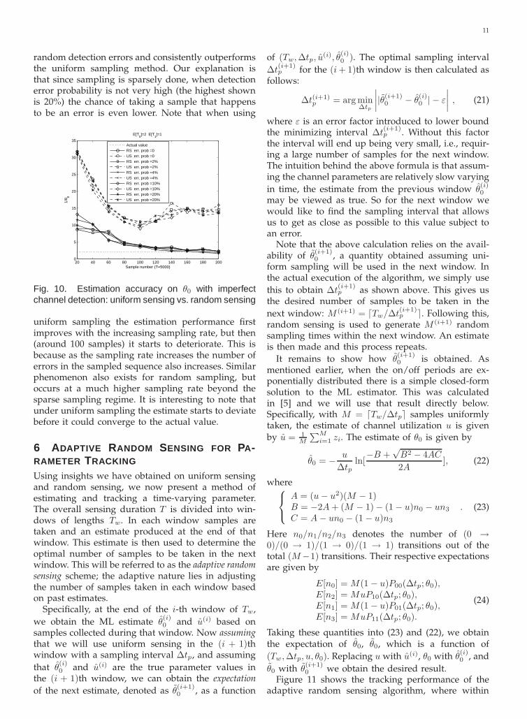
The results of applying our sensing algorithms totraces generated by this 3-state Markovian model areshown in Fig. 9, by using α = 0.7, p0 = 0.49, p1 =0.91, p2 = 0.06 (taken from [26]). In performing esti-mation we treated the channel as if it were a memory-less on/off channel which is not the case here due tothe two distinct on states. We see that random sensingagain outperforms uniform sensing.
10 20 30 40 50 60 70 80 90 1000
5
10
15
20
25
30
35
Sample number (T=5000)
1/θ 0
E[T0]=2.0451 E[T
1]=1.0792
Random samplingUniform samplingActual value
Fig. 9. Performance under a 3-state Markov model
5.5 Effect of channel state detection error
So far we have assumed that the channel state pro-cess Z(t) is perfectly detected. Fig. 10 shows theestimation performance in the presence of detectionerror. We inserted random detection errors into the 0-1 sequence with varying probabilities, and performedestimation using the revised sequence. The actualmean value refers to the sequence before error inser-tion. We see that random sampling is very robust to
11
random detection errors and consistently outperformsthe uniform sampling method. Our explanation isthat since sampling is sparsely done, when detectionerror probability is not very high (the highest shownis 20%) the chance of taking a sample that happensto be an error is even lower. Note that when using
20 40 60 80 100 120 140 160 180 2000
5
10
15
20
25
30
35
Sample number (T=5000)
1/θ 0
E[T0]=2 E[T
1]=1
Actual valueRS err. prob =0US err. prob =0RS err. prob =2%US err. prob =2%RS err. prob =4%US err. prob =4%RS err. prob =10%US err. prob =10%RS err. prob =20%US err. prob =20%
Fig. 10. Estimation accuracy on θ0 with imperfectchannel detection: uniform sensing vs. random sensing
uniform sampling the estimation performance firstimproves with the increasing sampling rate, but then(around 100 samples) it starts to deteriorate. This isbecause as the sampling rate increases the number oferrors in the sampled sequence also increases. Similarphenomenon also exists for random sampling, butoccurs at a much higher sampling rate beyond thesparse sampling regime. It is interesting to note thatunder uniform sampling the estimate starts to deviatebefore it could converge to the actual value.
6 ADAPTIVE RANDOM SENSING FOR PA-RAMETER TRACKING
Using insights we have obtained on uniform sensingand random sensing, we now present a method ofestimating and tracking a time-varying parameter.The overall sensing duration T is divided into win-dows of lengths Tw. In each window samples aretaken and an estimate produced at the end of thatwindow. This estimate is then used to determine theoptimal number of samples to be taken in the nextwindow. This will be referred to as the adaptive randomsensing scheme; the adaptive nature lies in adjustingthe number of samples taken in each window basedon past estimates.
Specifically, at the end of the i-th window of Tw,
we obtain the ML estimate θ(i)0 and u(i) based on
samples collected during that window. Now assumingthat we will use uniform sensing in the (i + 1)thwindow with a sampling interval ∆tp, and assuming
that θ(i)0 and u(i) are the true parameter values in
the (i + 1)th window, we can obtain the expectation
of the next estimate, denoted as θ(i+1)0 , as a function
of (Tw, ∆tp, u(i), θ
(i)0 ). The optimal sampling interval
∆t(i+1)p for the (i + 1)th window is then calculated as
follows:
∆t(i+1)p = arg min
∆tp
∣
∣
∣
∣
|θ(i+1)0 − θ
(i)0 | − ε
∣
∣
∣
∣
, (21)
where ε is an error factor introduced to lower boundthe minimizing interval ∆t
(i+1)p . Without this factor
the interval will end up being very small, i.e., requir-ing a large number of samples for the next window.The intuition behind the above formula is that assum-ing the channel parameters are relatively slow varying
in time, the estimate from the previous window θ(i)0
may be viewed as true. So for the next window wewould like to find the sampling interval that allowsus to get as close as possible to this value subject toan error.
Note that the above calculation relies on the avail-ability of θ
(i+1)0 , a quantity obtained assuming uni-
form sampling will be used in the next window. Inthe actual execution of the algorithm, we simply use
this to obtain ∆t(i+1)p as shown above. This gives us
the desired number of samples to be taken in the
next window: M (i+1) = ⌈Tw/∆t(i+1)p ⌉. Following this,
random sensing is used to generate M (i+1) randomsampling times within the next window. An estimateis then made and this process repeats.
It remains to show how θ(i+1)0 is obtained. As
mentioned earlier, when the on/off periods are ex-ponentially distributed there is a simple closed-formsolution to the ML estimator. This was calculatedin [5] and we will use that result directly below.Specifically, with M = ⌈Tw/∆tp⌉ samples uniformlytaken, the estimate of channel utilization u is given
by u = 1M
∑Mi=1 zi. The estimate of θ0 is given by
θ0 = − u
∆tpln[
−B +√
B2 − 4AC
2A], (22)
where
A = (u − u2)(M − 1)B = −2A + (M − 1) − (1 − u)n0 − un3
C = A − un0 − (1 − u)n3
. (23)
Here n0/n1/n2/n3 denotes the number of (0 →0)/(0 → 1)/(1 → 0)/(1 → 1) transitions out of thetotal (M −1) transitions. Their respective expectationsare given by
E[n0] = M(1 − u)P00(∆tp; θ0),E[n2] = MuP10(∆tp; θ0),E[n1] = M(1 − u)P01(∆tp; θ0),E[n3] = MuP11(∆tp; θ0).
(24)
Taking these quantities into (23) and (22), we obtainthe expectation of θ0, θ0, which is a function of
(Tw, ∆tp, u, θ0). Replacing u with u(i), θ0 with θ(i)0 , and
θ0 with θ(i+1)0 we obtain the desired result.
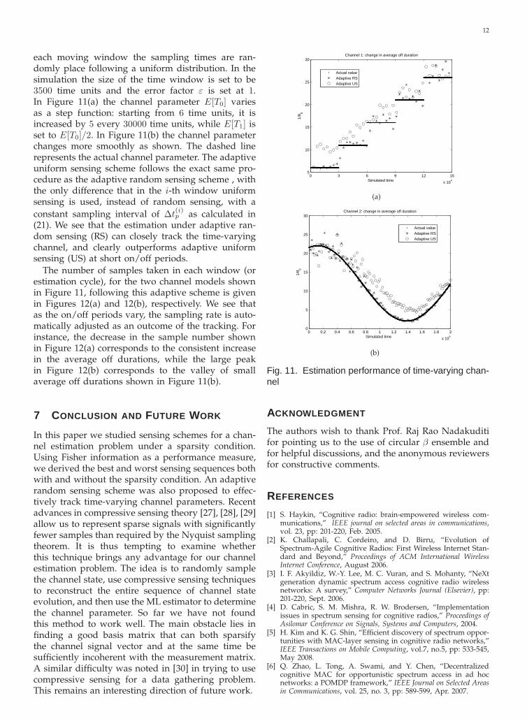
Figure 11 shows the tracking performance of theadaptive random sensing algorithm, where within
12
each moving window the sampling times are ran-domly place following a uniform distribution. In thesimulation the size of the time window is set to be3500 time units and the error factor ε is set at 1.In Figure 11(a) the channel parameter E[T0] variesas a step function: starting from 6 time units, it isincreased by 5 every 30000 time units, while E[T1] isset to E[T0]/2. In Figure 11(b) the channel parameterchanges more smoothly as shown. The dashed linerepresents the actual channel parameter. The adaptiveuniform sensing scheme follows the exact same pro-cedure as the adaptive random sensing scheme , withthe only difference that in the i-th window uniformsensing is used, instead of random sensing, with a
constant sampling interval of ∆t(i)p as calculated in
(21). We see that the estimation under adaptive ran-dom sensing (RS) can closely track the time-varyingchannel, and clearly outperforms adaptive uniformsensing (US) at short on/off periods.
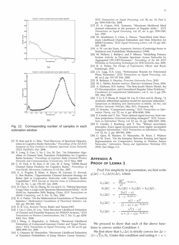
The number of samples taken in each window (orestimation cycle), for the two channel models shownin Figure 11, following this adaptive scheme is givenin Figures 12(a) and 12(b), respectively. We see thatas the on/off periods vary, the sampling rate is auto-matically adjusted as an outcome of the tracking. Forinstance, the decrease in the sample number shownin Figure 12(a) corresponds to the consistent increasein the average off durations, while the large peakin Figure 12(b) corresponds to the valley of smallaverage off durations shown in Figure 11(b).
7 CONCLUSION AND FUTURE WORK
In this paper we studied sensing schemes for a chan-nel estimation problem under a sparsity condition.Using Fisher information as a performance measure,we derived the best and worst sensing sequences bothwith and without the sparsity condition. An adaptiverandom sensing scheme was also proposed to effec-tively track time-varying channel parameters. Recentadvances in compressive sensing theory [27], [28], [29]allow us to represent sparse signals with significantlyfewer samples than required by the Nyquist samplingtheorem. It is thus tempting to examine whetherthis technique brings any advantage for our channelestimation problem. The idea is to randomly samplethe channel state, use compressive sensing techniquesto reconstruct the entire sequence of channel stateevolution, and then use the ML estimator to determinethe channel parameter. So far we have not foundthis method to work well. The main obstacle lies infinding a good basis matrix that can both sparsifythe channel signal vector and at the same time besufficiently incoherent with the measurement matrix.A similar difficulty was noted in [30] in trying to usecompressive sensing for a data gathering problem.This remains an interesting direction of future work.
0 3 6 9 12 15
x 104
5
10
15
20
25
30
Simulated time
1/θ 0
Channel 1: change in average off duration
Actual valueAdaptive RSAdaptive US
(a)
0 0.2 0.4 0.6 0.8 1 1.2 1.4 1.6 1.8 2
x 105
0
5
10
15
20
25
30
Simulated time
1/θ 0
Channel 2: change in average off duration
Actual valueAdaptive RSAdaptive US
(b)
Fig. 11. Estimation performance of time-varying chan-nel
ACKNOWLEDGMENT
The authors wish to thank Prof. Raj Rao Nadakuditifor pointing us to the use of circular β ensemble andfor helpful discussions, and the anonymous reviewersfor constructive comments.
REFERENCES
[1] S. Haykin, “Cognitive radio: brain-empowered wireless com-munications,” IEEE journal on selected areas in communications,vol. 23, pp: 201-220, Feb. 2005.
[2] K. Challapali, C. Cordeiro, and D. Birru, “Evolution ofSpectrum-Agile Cognitive Radios: First Wireless Internet Stan-dard and Beyond,” Proceedings of ACM International WirelessInternet Conference, August 2006.
[3] I. F. Akyildiz, W.-Y. Lee, M. C. Vuran, and S. Mohanty, “NeXtgeneration dynamic spectrum access cognitive radio wirelessnetworks: A survey,” Computer Networks Journal (Elsevier), pp:201-220, Sept. 2006.
[4] D. Cabric, S. M. Mishra, R. W. Brodersen, “Implementationissues in spectrum sensing for cognitive radios,” Proceedings ofAsilomar Conference on Signals, Systems and Computers, 2004.
[5] H. Kim and K. G. Shin, “Efficient discovery of spectrum oppor-tunities with MAC-layer sensing in cognitive radio networks,”IEEE Transactions on Mobile Computing, vol.7, no.5, pp: 533-545,May 2008.
[6] Q. Zhao, L. Tong, A. Swami, and Y. Chen, “Decentralizedcognitive MAC for opportunistic spectrum access in ad hocnetworks: a POMDP framework,” IEEE Journal on Selected Areasin Communications, vol. 25, no. 3, pp: 589-599, Apr. 2007.
13
0 3 6 9 12 15
x 104
150
200
250
300
350
400
450
500
Simulated time
Sam
ple
num
ber
Channel 1: number of samples taken by the adaptive algorithm
(a)
0 0.2 0.4 0.6 0.8 1 1.2 1.4 1.6 1.8 2
x 105
100
150
200
250
300
350
Simulated time
Sam
ple
num
ber
Channel 2: number of samples taken by the adaptive algorithm
(b)
Fig. 12. Corresponding number of samples in eachestimation window
[7] H. Kim and K. G. Shin, “Fast Discovery of Spectrum Opportu-nities in Cognitive Radio Networks,” Proceedings of the 3rd IEEESymposia on New Frontiers in Dynamic Spectrum Access Networks(IEEE DySPAN), Oct. 2008.
[8] X. Long, X. Gan, Y. Xu, J. Liu, M. Tao, “An Estimation Algo-rithm of Channel State Transition Probabilities for CognitiveRadio Systems,” Proceedings of Cognitive Radio Oriented WirelessNetworks and Communications (CrownCom), 15-17 May 2008
[9] C. H. Park, S. W. Kim, S. M. Lim, M. S. Song, “HMM BasedChannel Status Predictor for Cognitive Radio,” Proceedings ofAsia-Pacific Microwave Conference,11-14 Dec. 2007.
[10] A. A. Fuqaha, B. Khan, A. Rayes, M. Guizani, O. Awwad,G. Ben Brahim, “Opportunistic Channel Selection Strategy forBetter QoS in Cooperative Networks with Cognitive RadioCapabilities,” IEEE Journal on Selected Areas in Communications,Vol. 26, No. 1, pp: 156-167, Jan. 2008.
[11] D. Chen, S. Yin, Q. Zhang, M. Liu and S. Li, “Mining SpectrumUsage Data: a Large-scale Spectrum Measurement Study,” ACMMobiCom, September 2009, Beijing, China. IEEE Transactions onMobile Computing, vol. 8, No. 12, Dec. 2009.
[12] R. A. Fisher, “On the Mathematical Foundations of TheoreticalStatistics,” Mathematical Foundations of Theoretical Statistics vol.222, pp: 309-368, 1922.
[13] D. R. Cox, Renewal Theory, Butler and Tanner,1967.[14] J. Lee, J. Choi, H. Lou, “Joint Maximum Likelihood Estimation
of Channel and Preamble Sequence for WiMAX Systems,” IEEETransactions on Wireless Communications, Vol. 7, No. 11, pp: 4294-4303, Nov. 2008.
[15] J. Wang, A. Dogandzic, A. Nehorai, “Maximum LikelihoodEstimation of Compound-Gaussian Clutter and Target Param-eters,” IEEE Transactions on Signal Processing, vol. 54, no.10, pp:3884-3898 Oct. 2006.
[16] U. Orguner, M. Demirekler, “Maximum Likelihood Estimationof Transition Probabilities of Jump Markov Linear Systems,”
IEEE Transactions on Signal Processing, vol. 56, no. 10, Part 2,pp: 5093-5108 Oct. 2008.
[17] H. A. Cirpan, M.K. Tsatsanis, “Maximum likelihood blindchannel estimation in the presence of Doppler shifts,” IEEETransactions on Signal Processing, vol. 47, no. 6, pp: 1559-1569,Jun. 1999.
[18] M. Abuthinien, S. Chen, L. Hanzo, “Semi-blind Joint Maxi-mum Likelihood Channel Estimation and Data Detection forMIMO Systems,” IEEE Signal Processing Letters, vol. 15, pp: 202-205, 2008.
[19] A. W. van der Vaart, Asymptotic Statistics (Cambridge Series inStatistical and Probabilistic Mathematics) (1998)
[20] M. Wellens, J. Riihijrvi, and P. Mhnen, “Modelling PrimarySystem Activity in Dynamic Spectrum Access Networks byAggregated ON/OFF-Processes,” Proceedings of the 4th IEEEWorkshop on Networking Technologies for SDR Networks, Jun. 2009.
[21] R. A. Fisher, The Design of Experiments, Oliver and Boyd,Edinburgh, 1935.
[22] J.A. Legg, D.A. Gray, “Performance Bounds for PolynomialPhase Parameter,” IEEE Transactions on Signal Processing, vol.48, no.2, pp: 331-337 Feb. 2000.
[23] R. Bellman, S. Dreyfus, Princeton University Press, 2010.[24] M. L. Mehta, Random matrices. Elsevier/Academic Press, 2004.[25] A. Edelman, B.D. Sutton, “The Beta-Jacobi Matrix Model, the
CS Decomposition, and Generalized Singular Value Problems,”Foundations of Computational Mathematics, vol. 8 , no. 2, pp: 259-285, May 2008.
[26] Y. Li, S.-P. Sheng, R. Saigal, M. Liu, D. Chen and Q. Zhang, “Astochastic differential equation model for spectrum utilization,”Symposium on Modeling and Optimization in Mobile, Ad Hoc, andWireless Networks (WiOpt), May 2011, Princeton, NJ.
[27] D. Donoho, “Compressed sensing,” IEEE Transactions on Infor-mation Theory, vol. 52, no. 4, pp: 4036-4048, 2006.
[28] E. Candes and T. Tao, “Near optimal signal recovery from ran-dom projections: Universal encoding strategies?” IEEE Transac-tions on Information Theory, vol. 52, no. 12, pp: 5406-5425, 2006.
[29] E. Candes, J. Romberg, and T. Tao, “Robust uncertaintyprinciples: Exact signal reconstruction from highly incompletefrequency information,” IEEE Transactions on Information Theory,vol. 52, no. 2, pp: 489-509, 2006.
[30] G. Quer, R. Masiero, D. Munaretto, M. Rossi, J. Widmerand M. Zorzi, “On the Interplay Between Routing and SignalRepresentation for Compressive Sensing in Wireless SensorNetworks,” Information Theory and Applications Workshop (ITA2009), San Diego, CA.
APPENDIX APROOF OF LEMMA 1
Proof: For simplicity in presentation, we first writeg(∆t) = ho(∆t)h(∆t), where
ho(∆t) =∆t2
u2e−θ0∆t/u,
h(∆t) = h1(∆t) + h2(∆t) + h3(∆t) ,
h1(∆t) =2u(1 − u)
1 − e−θ0∆t/u,
h2(∆t) = − u(1 − u)2
(1 − u) + ue−θ0∆t/u,
h3(∆t) = − u2(1 − u)
u + (1 − u)e−θ0∆t/u.
We proceed to show that each of the above func-tions is convex under Condition 1.
We first show that ho(∆t) is strictly convex for ∆t >(2+
√2)u/θ0. Under this condition and noting 0 < u <
14
1 and θ0 > 0 we have
h′
o(∆t) =∆t
u2e−θ0∆t/u(2 − θ0∆t
u) < 0,
h′′
o (∆t) =e−θ0∆t/u
u2[(
θ0∆t
u− 2)2 − 2] > 0.
Therefore for θ0∆tu > 2+
√2, ho(∆t) is strictly convex.
That h1(∆t) is strictly convex is straightforward. Since0 < u < 1 and θ0 > 0, we have:
h′
1(∆t) =−2(1 − u)θ0e
−θ0∆t/u
(1 − e−θ0∆t/u)2< 0,
h′′
1 (∆t) =2(1 − u)θ2
0e−θ0∆t/u(1 + e−θ0∆t/u)
u(1 − e−θ0∆t/u)3> 0.
Next we show that h2(∆t) is strictly convex for∆t > u
θ0ln( u
1−u ). This condition is equivalent to
ue−θ0∆t/u < 1 − u. Under this condition and againnoting 0 < u < 1 and θ0 > 0, we have
h′
2(∆t) =−u(1 − u)2θ0e
−θ0∆t/u
[(1 − u) + ue−θ0∆t/u]2< 0,
h′′
2 (∆t) =(1 − u)2θ2
0e−θ0∆t/u[(1 − u) − ue−θ0∆t/u]
[(1 − u) + ue−θ0∆t/u]3
> 0.
Similarly, h3(∆t) is strictly convex under the condi-tion ∆t > u
θ0ln(1−u
u ), since
h′
3(∆t) =−u(1 − u)2θe−θ0∆t/u
[u + (1 − u)e−θ0∆t/u]2< 0,
h′′
3 (∆t) =(1 − u)2θ2e−θ0∆t/u[u − (1 − u)e−θ0∆t/u]
[u + (1 − u)e−θ0∆t/u]3
> 0.
Therefore under the condition ∆t > αu/θ0, h1,h2 and h3 are all monotonically decreasing convexfunctions. It follows that h = h1 + h2 + h3 is alsomonotonically decreasing and convex. Furthermore,for any ∆t > 0, ho(∆t) > 0, and h(∆t) > h(+∞) = 0.We can now show that g is strictly convex under thiscondition:
g′′
(∆t) = (ho(∆t)h(∆t))′′
= h′′
o (∆t)h(∆t) + 2h′
o(∆t)h′
(∆t)
+ho(∆t)h′′
(∆t) > 0 , (25)
where the inequality holds because every term on theright hand side is positive under the condition ∆t >αu/θ0 as summarized above.
Quanquan Liang received her B.S. degreeand Ph.D. in communication and informationsystems in the School of Information Sci-ence and Engineering, Shandong University,China, in 2004 and 2010. From 2008 to2010, she was with the Department of Elec-trical Engineering and Computer Science,University of Michigan, Ann Arbor, as a vis-iting student. Her research interests focus onwireless sensor networks and cognitive radionetworks.
Mingyan Liu Mingyan Liu received her Ph.D.Degree in electrical engineering from theUniversity of Maryland, College Park, in2000. She joined the Department of Elec-trical Engineering and Computer Science atthe University of Michigan, Ann Arbor, inSeptember 2000, where she is currently anAssociate Professor. Her research interestsare in optimal resource allocation, perfor-mance modeling and analysis, and energyefficient design of wireless, mobile ad hoc,
and sensor networks.
Dongfeng Yuan received his M. S. degreefrom Department of Electrical Engineering,Shandong University, China, 1988, and gothis Ph. D degree from Department of Electri-cal Engineering, Tsinghua University, Chinain 2000. Currently he is a full professor anddean in School of Information Science andEngineering, Shandong University, China.His research interests are in the area of wire-less communications, with a focus on cross-layer design and resource allocations.