Channel Characterization and Reliability of5.8 GHz DSRC Wireless CommunicationLinks in Vehicular Ad Hoc Networks in

Suburban Driving Environment

A thesis submitted in partial fulfillmentof the requirements for the degree of

Master of Sciencein

Electrical and Computer Engineeringat

Carnegie Mellon University

Jacob J. Meyers

Carnegie Mellon UniversityDepartment of Electrical and Computer Engineering

5000 Forbes AvenuePittsburgh, PA 15213, USA

09 May 2005(Revised 29 October 2005)

Key Words - VANET, vehicular ad hoc network, packet error rate, link reliability, suburban environment,

field test, channel characterization, path loss model., data distribution.

Abstract- A five node vehicular ad hoc network has been developed and used to model the

communications channel and estimate the packet error rate (PER) in real-world suburban driving

situations in varying traffic conditions. Measurements suggest that signal attenuation can be modeled

using the Log-Normal Path Loss Model with standard deviation of~ = 9.43 dB, but with an anomalously

low path loss exponent of n = 1.03. The reason for the low path loss exponent is not yet understood, but

data bias is suspected. Measurements also show a PER of 10% or less out to a distance of approximately

100 m, and indicate no strong correlation with relative or absolute velocities up to 48 KPH (30 MPH).

ACKNOWLEDGMENTS

I would like to offer special thanks to the following people for their involvement in this research effort.

Thanks to Dan Stancil (CMU) for serving as my academic advisor over the course of this project and

mentoring me as a student and a researcher. Thanks to Rahul Mangharam (CMU) and Dan Weller (CMU)

for the tremendous effort required to create and continually upgrade the software package used

throughout the research effort. Thanks to Jay Parikh (GM) for providing focus, guidance, support, and

encouragement on behalf of the research sponsors at General Motors.

Additional thanks to Suchit Mishra (CMU) and Kevin Borries (CMU) for driving during the many

collection efforts. Additional thanks to Raj Rajkumar (CMU), Christopher Kellum (GM), Hariharan

Krishnan (GM), Rajan Prasanna (GM), Priyantha Mudalige (GM), Vikas Kukshya (HRL), and Jijun

(HRL) for their suggestions and other guidance.

TABLE OF CONTENTS

Chapter One - Introduction ............................................................................................................................ l

Chapter Two - Description of Test Bed ........................................................................................................ 2

Description of Test Bed Hardware ................................................................................................................ 2

Description of Test Bed Software ................................................................................................................. 3

Chapter Three - Calibration of Radio Test Kits ......................................................................................... 6

Radio Test Kit Transmitter Calibration ........................................................................................................ 6

Radio Test Kit Receiver Calibration ............................................................................................................. 7

Chapter Four - Data Collection Techniques ................................................................................................ 8

Chapter Five - Empirical Results .................................................................................................................... 9

Basic Data Structuring and Calculations ........................................................................................................ 9

Data Analysis as a Function of Time and the Observation of Scenario Specific Data Features ............. 12

Channel Characterization .............................................................................................................................16

Data Analysis Techniques ........................................................................................................................17

Determination of Path Loss Exponent .................................................................................................... 19

Effects of Data Point Distribution "Clipping" ,on Data Analysis Results ............................................ 23

Determination of Standard Deviation of Gaussian Random Variable ................................................. 27

Link Reliability ..............................................................................................................................................29

Data Analysis Techniques ........................................................................................................................30

Determination of Link Reliability .......................................................................................................... 31

Chapter Six- Conclusions .............................................................................................................................33

Chapter Seven - Future Work ..................................................................................................................... 34

References ........................................................................................................................................................36

Appendix A- Transmitter Calibration Techniques .................................................................................. 38

Appendix B - Receiver Calibration Techniques ........................................................................................ 41

I. INTRODUCTION

The emergence and rapid commercialization of high-speed short-range wireless interfaces and low-cost

Global Positioning System (GPS) devices provides the opportunity to deploy a range of useful and

practical inter-vehicular communication applications. The integration of the Dedicated Short Range

Communications (DSRC) system in vehicles would enable the peer-to-peer communication required for

various proposed safety and emergency notifications and multimedia telematics applications [1,2].

Unfortunately, there has been very little realistic field testing of vehicular ad hoc networks (VANETs)

using the IEEE 802.1 lp protocol in dynamic mobile environments. Consequently, the large scale path

loss of the communications channel between nodes has not been accurately modeled using empirical data,

and the performance and reliability of such networks are not well understood in real-world driving

environments.

J. Maurer, et al. describe a set of real-world field experiments using narrow-band measurements at 5.2

GHz [3] similar to those presented in this thesis, however, they only use a single link between two

vehicles. Furthermore, link reliability with respect to packet error rates is not addressed. In addition, their

efforts to model the channel focus on fading statistics, Doppler analysis, and level crossing rate, but do

not address large scale path loss as function of distance. X. Zhao, et al. characterized wideband outdoor

mobile communications signal propagation at 5.3 GHz using techniques very similar to those described in

this thesis [4], however, they used a stationary transmitting node and a mobile receiving node rather than

an ad hoc vehicle-to-vehicle network and did so at a frequency below that of the new IEEE 802.1 l p band.

Likewise, T. Schwengler and M. Gilbert as well as G. Durgin, et al. conducted experiments at 5.8 GHz in

residential neighborhoods [5,6] very similar to those presented in this thesis; however, as was the case

with X. Zhao, et al., they used a stationary transmitting node and a mobile receiving node rather than an

ad hoc vehicle-to-vehicle network.

A. Visser, et al. developed a hierarchical method of modeling the reliability of DSRC links for electronic

toll collection applications [7]; however their model was specifically for stationary node to moving

vehicle links and does not apply to vehicle-to-vehicle communications networks. In addition, their results

were based solely on simulations, and were not validated using realistic field testing. Likewise, M.

Torrent-Moreno, et al. and J. Yin et al. have shown simulation results using a 5.8 GHz DSRC vehicular

ad hoc network with a reasonable estimate of link reliability [8,9]. However, the simulation utilized a

theoretical large scale path loss model and the results were not validated using realistic field testing.

The General Motors Collaborative Research Laboratory Ad Hoc Networking Project Team at Carnegie

Mellon University has developed a five node test-bed platform to collect the real-world data needed to

develop RF channel propagation models and VANET routing protocols for realistic driving situations [1 ].

This thesis discusses the composition of the platform, data collection and analysis techniques, and the

findings and conclusions about the channel characterization and the reliability of the individual links

between networked vehicles in suburban driving environments.

II. DESCRIPTION OF TEST BED

Each node in the ad hoc network presented in this thesis corresponds to one of five vehicles equipped

with a radio test kit.

A. Description of Test Bed Hardware

Unlike J. Maurer, et al. and G. Durgin, et al. who used signal generators and spectrum analyzers to make

their channel measurements, [3,6], the wireless vehicular networking test-bed used to collect the data

presented in this thesis was created using commercially available communications equipment.

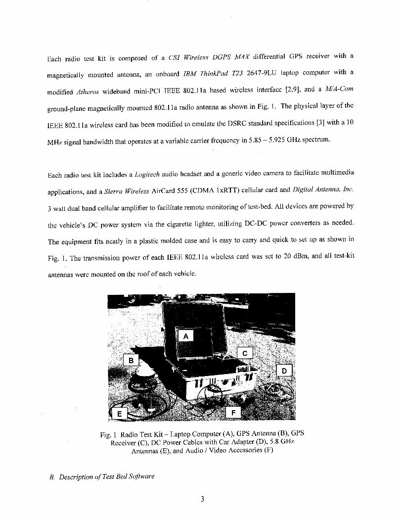
Each radio test kit is composed of a CSI Wireless DGPS MAX differential GPS receiver with a

magnetically mounted antenna, an onboard IBM ThinkPad T23 2647-9LU laptop computer with a

modified Atheros wideband mini-PCI IEEE 802.11a based wireless interface [2,9], and a M/A-Com

ground-plane magnetically mounted 802.1 la radio antenna as shown in Fig. 1. The physical layer of the

IEEE 802.1 la wireless card has been modified to emulate the DSRC standard specifications [3] with a 10

MHz signal bandwidth that operates at a variable carrier frequency in 5.85 - 5.925 GHz spectrum.

Each radio test kit includes a Logitech audio headset and a generic video camera to facilitate multimedia

applications, and a Sierra Wireless AirCard 555 (CDMA lxRTT) cellular card and Digital Antenna, Inc.

3 watt dual band cellular amplifier to facilitate remote monitoring of test-bed. All devices are powered by

the vehicle’s DC power system via the cigarette lighter, utilizing DC-DC power converters as needed.

The equipment fits neatly in a plastic molded case and is easy to carry and quick to set up as shown in

Fig. 1. The transmission power of each IEEE 802.11 a wireless card was set to 20 dBm, and all test-kit

antennas were mounted on the roof of each vehicle.

Fig. 1 Radio Test Kit - Laptop Computer (A), GPS Antenna (B), Receiver (C), DC Power Cables with Car Adapter (D), 5.8

Antennas (E), and Audio / Video Accessories (F)

B. Description of Test Bed Software

Rahul Mangharam and Daniel Weller, both members of the General Motors Collaborative Research

Laboratory at Carnegie Mellon University, developed the GTK RoadMap software package used in this

research project. The GTK RoadMap software tracks vehicle locations on a virtual map, operates the

wireless communications hardware package, and records measured data. The onboard laptop computer in

each radio test kit runs Red Hat Linux Version 9 (Kernel 2.4.18-3) which provides a fertile platform for

network protocol and application development. There are primarily three layers of software, built from

open source libraries.

Runtime display capability l"or multiple vehicles was added to the original the GTK RoadMap software

tool [4] used by the test-bed so that the current location and movement of all vehicles in the network can

be visually tracked as they are driven. Communi[cations capability was added so that each vehicle’s

onboard computer can act as, a server and accept c,~nnections from other vehicles. Each computer runs a

User Datagram Protocol (UDP) client thread to connect to all other computers in the test-bed. The

connections occur at the socket level; therefore, the application manages the end-to-end data exchange

between each client and server. The client and server connections are displayed in a panel at the base of

the user interface. The underlying kernel-based networking software handles multi-hop routing along the

set of links between the client and server.

GPS location coordinates are computed five times per second and have an accuracy of < 2m. The

transmission of each data packet coincides with the computation of each set of location coordinates;

therefore, data packets are exchanged five times per second as well.

Using this client-server setup, each vehicle in the network exchanges data packets with headers

specifically designed for the efficient exchange of position and network information. Each transmitted

packet header contains the fbllowing data: packet number, packet size, transmitter IP address, time the

packet was transmitted, the longitude, latitude, and altitude of the transmitting vehicle, the speed and

heading of the transmitting vehicle, RF channel, data transmission rate [Mbps], and transmitted signal

strength as well as source and destination routing information and GPS receiver statistics. The packet

pa.yload is utilized to send both critical information such as emergency messages and non-critical

information such as voice and video, multimedia, and application data.

The onboard computer in each test kit logs the GPS and network data contained in the header of both

transmitted and received packets. The logged value transmitted signal strength field for each received

packet is replaced by the measured received signal strength or RSSI. In addition, the packet origin (local

or network) and the distance from the transmitting node to the node at which the data is logged is

included in the data log. This; distance value is zero for all logged transmitted packets and non-zero tbr all

logged received packets.

These data logs enable the playback of the route driven, at either actual speed or a user defined higher

speed, and the visualization of the vehicles on a vector-based rendering of the map traversed. The

mapping functions utilize TIGER/Line 2002 data files available from the U.S. Census Bureau [1 I]. In

addition, the raw data can also be used for external post-processing and analysis.

Within the data logs, transmitted packets are differentiated from received packets by the "packet origin"

field - "local" packets were transmitted by the node at which the packet was logged and "network"

packets were transmitted by some other node in the network. The identity of the transmitting node is

specified in the "transmitter [P address" field. The location, speed, and heading data of all packets is thai

of the node from which the packets were transmitted, therefore, when the data is processed, the location,

speed, and heading data of the received packets must be interpolated from the nearest transmitted packet

data entries in the log of that particular node.

Each node also has the calz, ability of using the AODV ad hoc networking protocol [1,10], but packet

relaying was not used for collecting the data reported here. Consequently, the results we report apply to

single hop links.

IlL CALIBRATION OF RADIO TEST KITS

The transmitted signal strength for all packets sent from any radio test kit can be specified by the user in

terms of a "ForcePower" index value, and the received signal strength of the all packets received by any

radio test kit are measured in terms of an "RSSI" index value. In order for these index values to have an5’

meaningful value in measuring signal attenuation, they had to be calibrated in terms of a physical power

value [dBm] for each radio test kit.

A. Radio Test Kit Transmitter Calibration

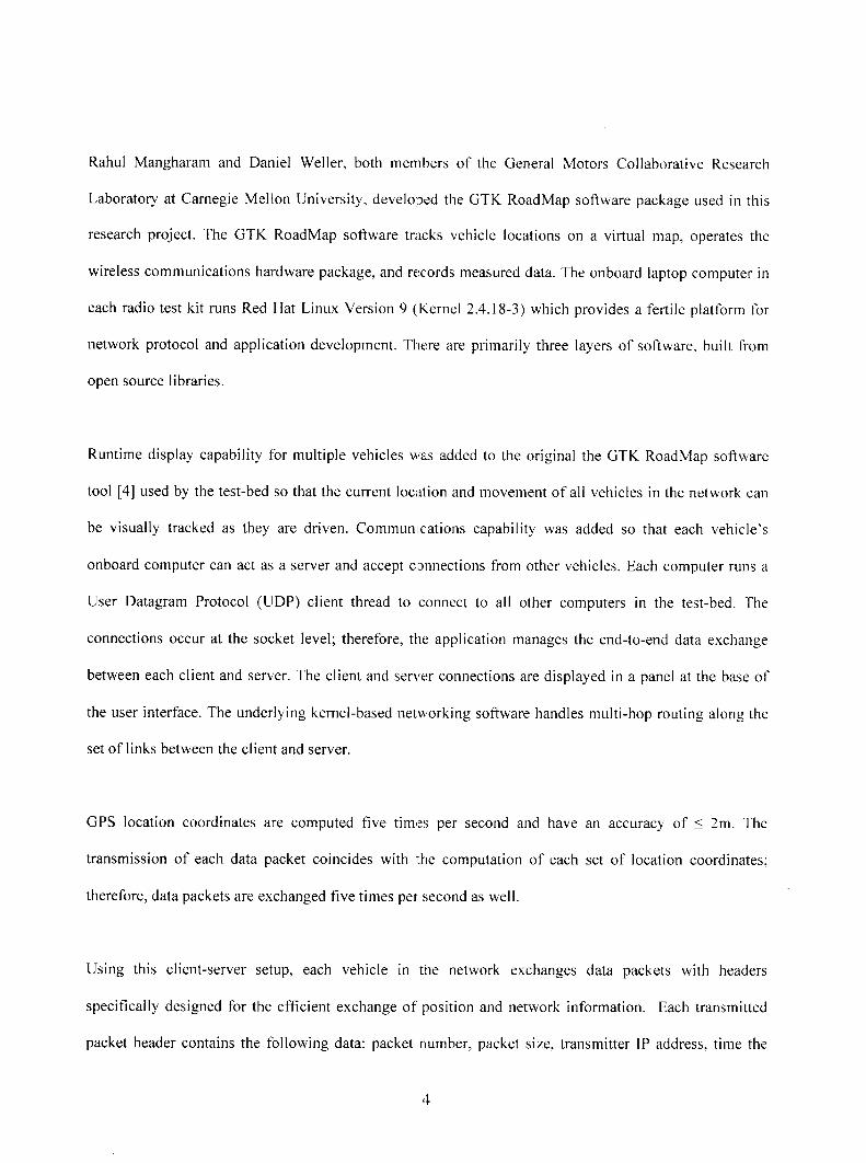
Each radio test kit’s transmitted power was calibrated using another radio test kit, a signal detector, an

attenuator, an oscilloscope, and a signal generator. The power transmitted at each "ForcePower" setting

was determined by measuring the amount of power required to create a square-wave-modulated signal of

the same frequency and magnitude using the signal generator. Five iterations of such measurements were

averaged at each "ForcePower" setting to generate the corresponding transmitted power value [dBm]. The

calibration table of "ForcePower" index values and the corresponding overall average power values

[dBm] is shown graphically in Fig. 2. Appendix A provides additional details about the transmitter

calibration process.

rewoP

d

t

snarT

24~ GM-2

i GM-3

22

20

18

16

14

10~ ¯

R ....20 25 3o~ ~5

ForcePower Index40 45 5O

Fig. 2 Measured Transmitted Power vs. ForcePower Index of the FiveRadio Test Kits (GM-I to GM-5) Used in the Research Project

B. Radio Test Kit Receiver Calibration

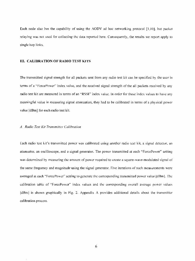
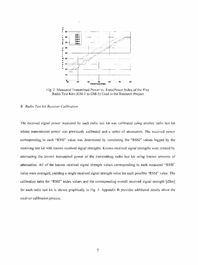
The received signal power measured by each radio test kit was calibrated using another radio test kit

whose transmission power was previously calibrated and a series of attenuators. The received power

corresponding to each "RSSI" value was determined by correlating the "RSSI" values logged by the

receiving test kit with known received signal strengths. Known received signal strengths were created by

attenuating the known transmitted power of the transmitting radio test kit using known amounts of

attenuation. All of the known received signal strength values corresponding to each measured "RSSI"

value were averaged, yielding a single received signal strength value for each possible "RSSI" value. The

calibration table for "RSSI" index values and the corresponding overall received signal strength [dBm]

for each radio test kit is shown graphically in Fig. 3. Appendix B provides additional details about the

receiver calibration process.

7

!

rew0P

devie¢

R

-20 ~

Model-30 GM-1

GM-2GM-3

-40 GM-4GM-5

-50

-60~

-1°°o lO 20

+

+

30 40 50 60 70 80RSSI Index

Fig. 3 Actual Received Power vs. RSSI Index lbr Each Radio TestKit (GM-1 to GM-5) Compared With the Model Given by Eq. (1)

For the most part, the calibrated received signal strength values were consistent with the model (1)

provided with the radio cards for "RSSI" values between 20 and the upper end of the range of values.

P~[dBm]= RSSI - 95 (1)

IV. DATA COLLECTION TECHNIQUES

The data presented in this thesis was collected in suburban driving environments, characterized by one or

two story buildings and residential streets. Each data set represents approximately one hour of driving

time. The radio test-kits were set up for broadcast transmission such that a single transmission can be

received by N-I receivers, where N was the number of nodes involved in the test run. The packet

transmission rate was five times per second and was equal to the rate at which the GPS receiver unit

updates location, speed, and heading data.

The data set presented in this. paper contains over 625,000 communications link measurements taken over

the course of multiple days. These measurements required approximately five hours of driving time, and a

combination of 38 individual node-to-node links while driving various numbers of vehicles in a convoy-

like formation through the Squirrel Hill, Shadyside, Oakland, and Bloomfield residential neighborhoods

in Pittsburgh, PA.

V. EMPIRICAL RESULTS

A. Basic Data Structuring and Calculations

As previously mentioned, the location, (absolute) speed, and heading data of all logged packets was that

of the node from which the packets were transmitted, therefore, the logged received packet data provided

no information about the point at which the packet was received. Once each data log was parsed, the

location, (absolute) speed, and heading data for each received packet was replaced with the logged

location, (absolute) speed, and heading data of the packet transmitted from the receiving node at the same

time that the incoming packet was received. The information about the point from which the packets were

transmitted is preserved in each data log. After the data replacement procedure was complete, the data

was divided into data sets for transmitted and received packets. The data set for received packets was then

subdivided by the transmitter’ from which they originated.

Before the transmitted and received signal strength values could be used for any data analysis, they had to

be converted from the "ForcePower" and "RSSI" index values into physical power values [dBm]. The

power value conversion was accomplished by using a "look-up" table approach. A search was conducted

for the "ForcePower" index value of each transmitted packet in the corresponding transmitter calibration

table. Once the "ForcePower" index value was located in the table, the corresponding transmitted power

[dBm] value was used to replace the "ForcePower" index value for that particular packet in the matrix of

transmitted packet data. Likewise, the "RSSI" index values were replaced with the received power [dBm]

values contained in the corresponding receiver calibration table.

At this point, the packets transmitted from Test-Kit A were matched up with the packets received by Test-

Kits B,C,D, and E which were known to have originaled from Test-Kit A using the packet number

information. The resulting matrix of transmitted packet - received packet pairs represented the "received

packets" data set for that particular link. All packets transmitted from one test-kit for which there was no

received packet at any one ol~the other test kits was considered a "dropped packet" for that particular link.

By definition, there were N-1 links for each transmitter - one to each of the other test kits. Each of these

links was evaluated individually, therefore the number of packets received by or dropped en route to any

other given test-kit was independent of that of all other test-kits.

The distance between any two given nodes was determined using the Haversine formula (2), given the

latitude and longitude of each node [11]:

ALat = Lat~_ - Lat~

ALong = Long~_ - Long~

a-- sin +cos(Latl)’cos(Lat2)" sinng

(2)

c = 2"atan2 (~-,~-)1

Distance = R ̄ c

where R = 6,373,000 [m] is the radius of the earth optimized for locations approximately 39° from the

equator.

10

If a packet was dropped, the location of the intended receiving unit, and thus the distance between the two

nodes, and other pertinent information could only be estimated. Since the packets containing the location,

speed, and heading data were transmitted five times per second, it was assumed that the validity of this

data for any given node would not be significantly degraded if fewer than five consecutive packets were

dropped if the nodes were moving at reasonable speeds. The location, speed, and heading of the intended

receiving unit for dropped packets were therefore assigned the values of the last successfully received

packet if there was less than one second time differential between the times at which the two packets were

transmitted. Unfortunately, the received signal strength of dropped packets cannot be accurately estimated

at this time due to the unknown behavior of fast-fading effects.

One goal of the project was to determine a large-scale fading model for the 5.8 GHz peer-to-peer channel.

To isolate the large-scale fading behavior, the effects of fast fading were removed using a sliding average

of the received signal strength measurements as a function of time. This sliding average was implemented

by sequentially assigning each transmitted and received data packet in the entire data set the average

value of itself and any packets transmitted and received within a one second margin centered about the

time value of the given packet. Due to the fact that the averaging of the signal strength data was done with

respect to a given time period, the transmitted and received power values had to be converted from the

logarithmic scale to the linear scale prior to being averaged, and then converted from the linear scale back

to the logarithmic scale to be consistent with the rest of the signal strength data analysis.

Distance and speed measurements do not exhibit fast fading effects; however, the accuracy of the GPS

location and speed measurements does vary as a fi~nction of the number of satellites available and other

such factors. The sliding aw,~rage technique used to filter out the fast-fading effects on received signal

strength measurements was equally useful for minimizing the effects of less than accurate location and

speed data measurements.

11

The velocity of any two nodes relative to each other was determined by calculating the change in the

distance between those two nodes from one received packet to the next divided by the time elapsed

between transmission of the two packets. By definition, a positive relative velocity indicates that the

nodes were moving away from each other, while a :negative relative velocity indicates that the nodes were

moving towards each other.

In most cases, it was useful to separate the data collected while the vehicles were stationary from the data

collected while they were in motion. While the vehicles were stationary, but actively collecting data, the

data points corresponding to specific distance and signal attenuation values accumulated in large numbers

inconsistent with the typical distribution of data collected while vehicles were in motion. Separation of

these data points was accomplished by creating a temporary data matrix containing only the data

corresponding to packets in the matrix of transmitted and received packet pairs that were transmitted

while either the transmitting node or the receiving node (or both) had a speed value greater than zero.

B. Data Analysis as a Function of Time and the Observation of Scenario Specific Data Features

Although the objective of this research effort was to characterize the channel and evaluate the link

reliability on a large scale that encompasses all driving siluations in suburban environments, it was often

desirable to relate a particular data set to the specific route followed while collecting the data. The

simplest way to evaluate ’such effects was to simply play back the logged sequence of packet

transmissions. The GTK RoadMap program allows users replay past data logs, both at normal speed and

at several times the normal :speed, retracing the exact path of each vehicle on the GTK RoadMap user

interface map. There are four major data variables that, when plotted as a function of time, directly link

system performance metrics to individual scenarios shown on the GTK RoadMap data log replays.

12

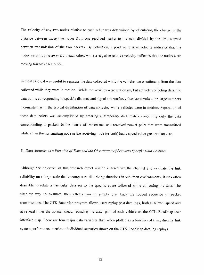
First, plots of the packet numbers of packets received and dropped over the course of time as well as the

cumulative number of each, as shown in Fig. 4, clearly indicate the points in time at which the pattern of

packets received and dropped was interrupted. For the most part, it was observed that the dropped packets

came in bursts that corresponded to situations such as vehicles getting temporarily separated from each

other or large obstructions between vehicles blocking line-of-sight signal paths. In addition, the

cumulative number of packets received and dropped plotted on the same time scale shows how the effects

of the lost packets adds up over time and provides an over all percentage of packets received and dropped

over the course of the entire data set. These overall performance statistics include only those packets

transmitted while the receiw:rs of each of the other radio test kits were enabled, so that packets sent to a

radio test kit which was turned off were not counted as dropped packets.

15000

rebrnuN 10000

t

caP 5000

I .... Totai Packets ReceivedPackets Received

°o~ ............ ~- ~o 4’0Time [rnin=Jtes]

15000~ : ~l-PacketsDro~oed

N 10000

50 60 0 10 20 30 40 50Time [minutes]

(A) (B)

Fig. 4 Packets Received By GM-3 From GM-4 and Cumulative Received (A)

(Packets Sent = 15662, Packets Received = 15074, Percent Received = 96.2457)and Packets Dropped From GM-4 and Cumulative Dropped (B) vs. Time

(Packets Sent = 15662, Packets Dropped = 588, Percent Dropped = 3.7543)in Squirrel Hill Neighborhood on 11 November 2004

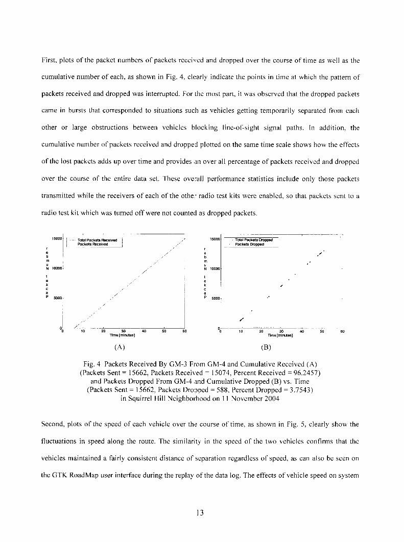
Second, plots of the speed of each vehicle over the course of time, as shown in Fig. 5, clearly show the

fluctuations in speed along the route. The similarity in the speed of the two vehicles confirms that the

vehicles maintained a fairly consistent distance of separation regardless of speed, as can also be seen on

the GTK RoadMap user interface during the replay of the data log. The effects of vehicle speed on system

13

performance are primarily related to Doppler effects and fast-fading, and can be filtered out of the

measured signal strength data for channel modeling purposes as described above; however, they cannot

be physically eliminated from the channel, and therefore contribute to the lost packet behavior. The

relevance of vehicle speed data analysis lies in the significant effects that such fast-fading behavior can

have on the packet error rate of the communications link as discussed later in this thesis.

40

35]

30Pm[ 25

de 2O

PS 15

GM-4 (Transmitter)GM-3 (Receiver)

10

030 35 40 45 50

Time [min]

Fig. 5 Speed of a Typical Radio Test Kit Transmitter (GM-4) And Receiver(GM-3) vs. Time in Squirrel Hill Neighborhood on 11 November 2004

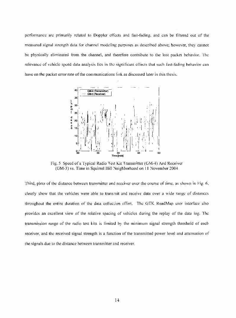
Third, plots of the distance between transmitter and receiver over the course of time, as shown in Fig. 6,

clearly show that the vehicles were able to trans~rnit and receive data over a wide range of distances

throughout the entire duration of the data collection effort. The GTK RoadMap user interface also

provides an excellent view of the relative spacing of vehicles during the replay of the data log. The

transmission range of the radio test kits is limited by the minimum signal strength threshold of each

receiver, and the received signal strength is a function of the transmitted power level and attenuation of

the signals due to the distance between transmitter and receiver.

14

e 160II

0 10 20 30 40 50 60T~me [min]

Fig. 6 Distance Between Transmitter (GM-4) And Receiver (GM-3) vs. in Squirrel Hill Neighborhood on 11 November 2004

The plot of the distance between transmitter and receiver over the course of time provides a great deal of

insight when overlaid with tlhe plots of other system performance metrics which are a function of distance

on the same time scale.

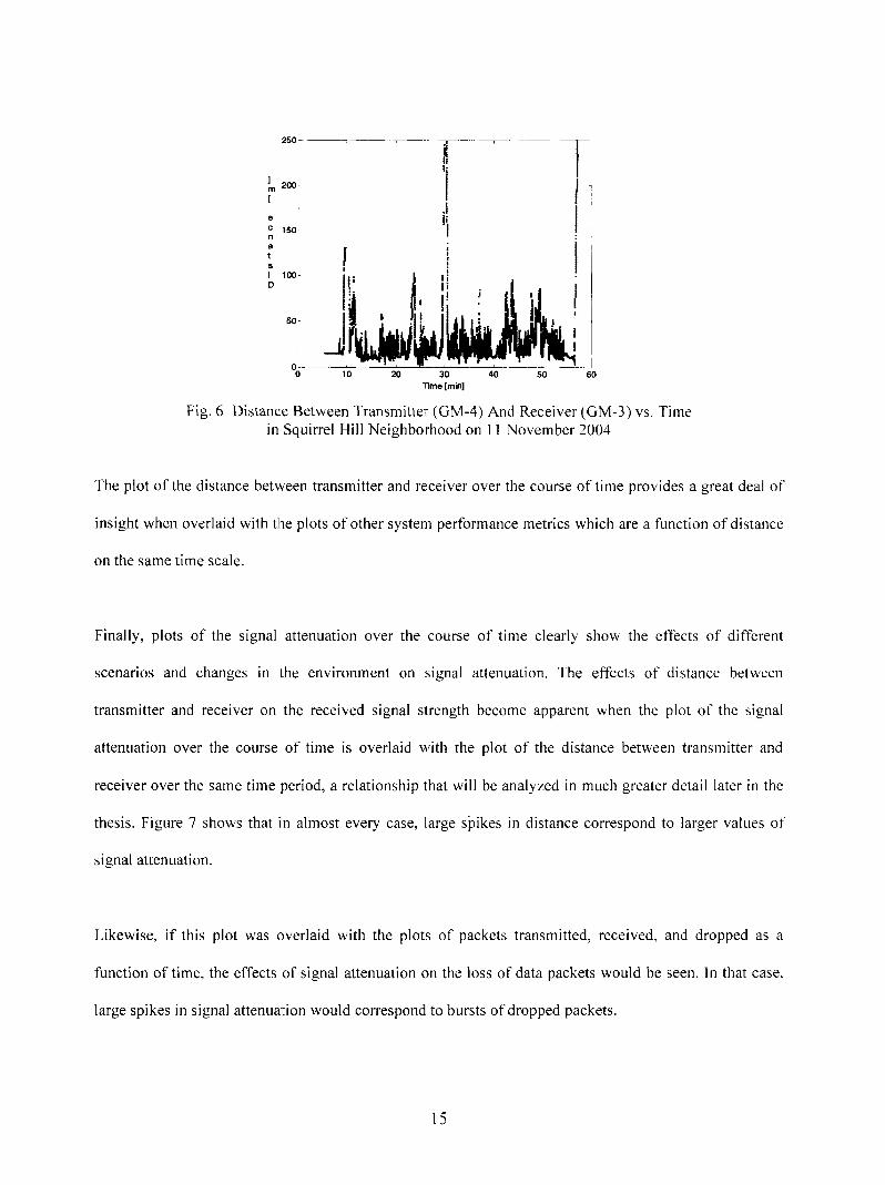
Finally, plots of the signal attenuation over the course of time clearly show the effects of different

scenarios and changes in the environment on signal attenuation. The effects of distance between

transmitter and receiver on the received signal strength become apparent when the plot of the signal

attenuation over the course of time is overlaid with the plot of the distance between transmitter and

receiver over the same time period, a relationship that will be analyzed in much greater detail later in the

thesis. Figure 7 shows that in almost every case, large si~ikes in distance correspond to larger values of

signal attenuation.

Likewise, if this plot was overlaid with the plot.,; of packets transmitted, received, and dropped as a

function of time, the effects of signal attenuation on the loss of data packets would be seen. In that case,

large spikes in signal attenuation would correspond to bursts of dropped packets.

15

250120

110,

100!

9O

80

70

OL

~me [mini

2001n

[

e

150c

100i

Fig. 7 Signal Attenuation and Distance Between Transmitter(GM-2) and Receiver (GM-3) vs.

in Squirrel Hill Neighborhood on 11 November 2004

C, Channel Characterization

As suggested above, overlaying the various plots of system performance variables vs. time shows how the

different variables are closely related to each other. Another excellent way to observe these relationships

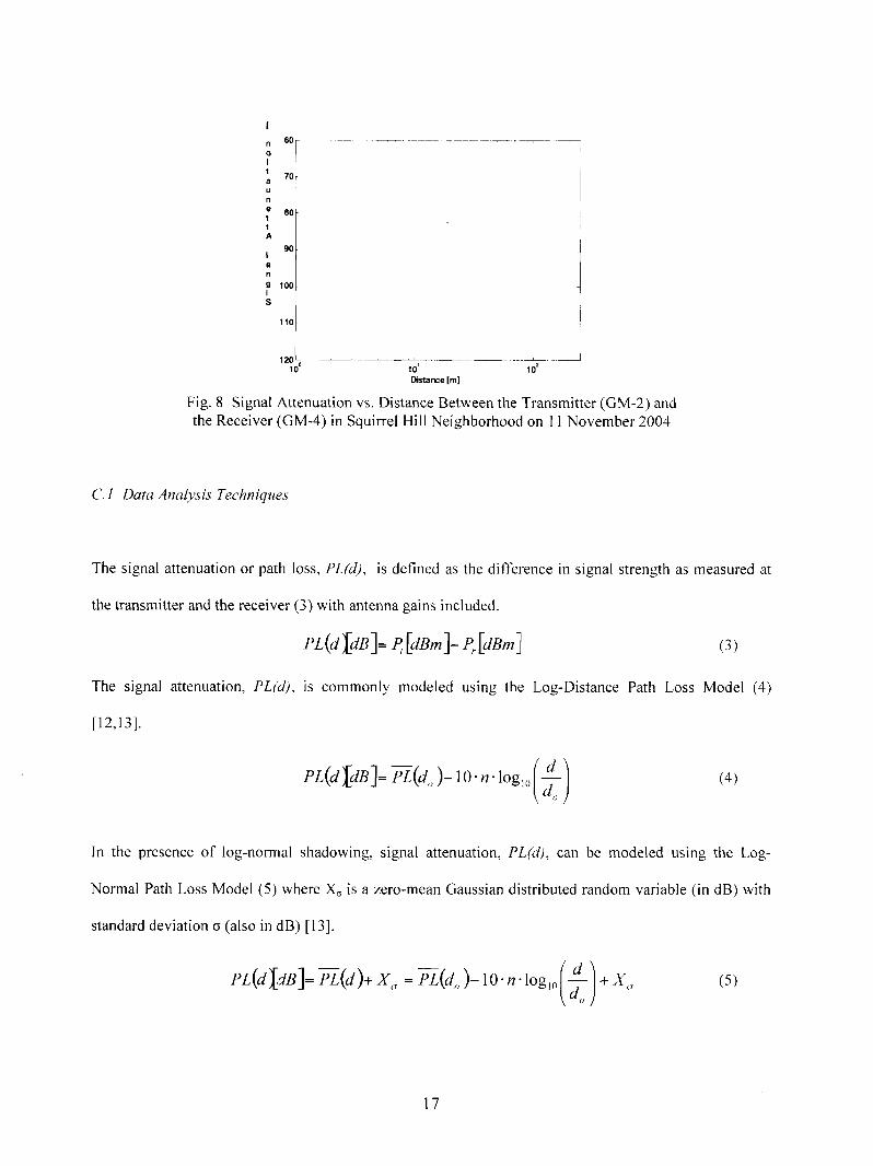
is to plot one variable as a function of the other. For example, a plot of signal attenuation vs. distance

between transmitter and receiver as shown in Fig.. 8 provides a different perspective on the same data

presented in Fig. 7. It also shows two distinct things about the nature of the relationship between signal

attenuation and distance - there is a general increase in signal attenuation as the distance increases, and

there is a distribution of signal attenuation data points at each distance - which provide the foundation for

the channel characterization model used in this thesis.

16

10~102

Distance [m]

Fig. 8 Signal Attenuation vs. Distance Between the Transmitter (GM-2) andthe Receiver (GM-4) in Squirrel Hill Neighborhood on 11 November 2004

C. 1 Data Analysis Techniques

The signal attenuation or pallh loss, PL(d), is defined as the difference in signal strength as measured at

the transmitter and the receiver (3) with antenna gains included.

The signal attenuation, PL(d), is commonly modeled using the Log-Distance Path Loss Model (4)

[12,13].

PL(d~_dB]~-fi-~(d,, )- lO’n’log~oZ (4)

In the presence of log-normal shadowing, signal attenuation, PL(d), can be modeled using the Log-

Normal Path Loss Model (5) where Xo is a zero-mean Gaussian distributed random variable (in dB)

standard deviation ~ (also in riB) [13].

X,, = )- lO’n.log,o( d ) + x,,

17

If the signal attenuation is measured using logarilhmic units [dB] and the distance is converted from the

linear scale to the logarithmic scale, the modeled path loss will be a straight line with a slope of 10n dB

per decade of distance. The value of the path loss exponent, n, can be calculated using a linear regression

of the empirical data points over a wide range of distances between transmitter and receiver. The standard

deviation, ~, of the zero-me, an Gaussian random variable can be determined using the standard deviation

of the distribution of data points at each distance.

Due to the very large number of data points in each data set, the distribution of all measured signal

attenuation data points at each distance was represented by its mean value when calculating the path loss

exponent, n, for the Log-Distance Model. Since the mean signal attenuation values at each distance were

used in the linear regression to calculate the va]lue of the path loss exponent, n, then E(X~) = 0

definition, and, if d(, = 1, the Log-distance Path Loss Model can be rewritten as (6) where PLO) is a

constant offset value.

-fi-£(d )[dB ]= - l O " n " l°g,o (d )+ -~0 (6)

The channel characterization described above was determined for each transmitter-receiver link in the

following way. First, the range of possible distances between transmitters and receivers was divided up

into one meter segments corresponding with integer distance values, each with a 0.1 meter margin to

either side forming a "bin." Second, at each distance value, all data packets in the matrix of transmitted

and received packet pairs that were received while the nodes were at a distance within the given bin were

identified and counted. Third, the signal attenuation for each packet transmitted over the given distance

was calculated by subtracting the received signal strength from the transmitted signal strength (3). Fourth,

the sum of all signal attenuation values was divided by the total number of packets transmitted at the

given distance to determine the average signal attenuation. Finally, after calculating the average signal

attenuation value for each of’ the distances, the path loss exponent, n, and the constant offset value in the

18

Log-Distance Path Loss Model (6) were calculated for each link in the individual data set using a l~rst

order polynomial (linear) regression of the form (7):

y = a0 +t’a~ (7)

in which

y = -fi~(d ldB ] (7.a"

a 0 = |Ogl0 ~0)) (7.b)

a1 = 10 ̄ log,0 (d) (7.c)

(7.d)

After determining the path loss exponent, n, and the constant offset value for each of the links in all of the

individual data sets, a matrix of the distance values., the sum total measured signal attenuation values, and

the sum total number of packets transmitted at each distance was created for each link in the individual

data set, and the data contained in all of these matrices was aggregated into a single data set. The overall

average signal attenuation at each distance was calculated by dividing the sum of the total signal

attenuation values by the sum of the total number of packets transmitted at each distance from all of the

links. The overall path loss exponent, n, and the constant offset value in the Log-distance Path Loss

Model (6) were calculated for all links using the same first order polynomial (linear) regression technique

(7).

C.2 Determination of Path Loss Exponent

The average signal attenuati.c)n [dB] and the number of time averaged measured signal attenuation data

points for vehicles in motion used to calculate that average at each distance are shown in Fig. 9 using the

same logarithmic distance (horizontal) axis. The average signal attenuation data points over the range

19

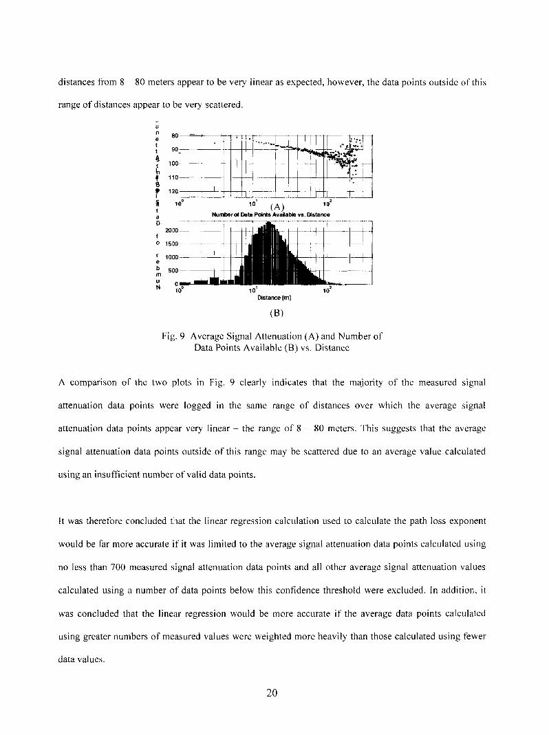
distances from 8 - 80 meters appear to be very linear as expected, however, the data points outside of this

range of distances appear to be very scattered.

u

tt

t

taD

fo

uN

100

110

120

100

15 O0

1000

500

~o’ (A) ~o’Number of Data Points Available vs. Distance

10t 102

Distance [m]

(B)

Fig. 9 Average Signal Attenuation (A) and Number Data Points Available (B) vs. Distance

A comparison of the two plots in Fig. 9 clearly indicates that the majority of the measured signal

attenuation data points were logged in the same range of distances over which the average signal

attenuation data points appear very linear - the range of 8 - 80 meters. This suggests that the average

signal attenuation data points outside of this range may be scattered due to an average value calculated

using an insufficient number of valid data points.

It was therefore concluded that the linear regression calculation used to calculate the path loss exponent

would be far more accurate if it was limited to the .average signal attenuation data points calculated using

no less than 700 measured signal attenuation data points and all other average signal attenuation values

calculated using a number of data points below this confidence threshold were excluded. In addition, it

was concluded that the linear regression would be more accurate if the average data points calculated

using greater numbers of measured values were weighted more heavily than those calculated using fewer

data values.

20

The weighting of average signal attenuation values was accomplished using the following technique.

First, the "weight" was defined as the total number of measured signal attenuation data points at each

distance divided by one fourth of the minimum number of data points specit]ed above and rounded up to

the nearest integer value. This definition of the "weight~’ given to each average signal attenuation data

point was arbitrarily derived from the need to reduce the number of total data points used in the linear

regression from several thousand to several hundred while providing enough resolution that the weighting

effect was significant. Second, the average signal attenuation value corresponding to each distance was

placed in the array of average signal attenuation values the "weight" number of times. Finally, the

distance value was placed in the array of distance values the "weight" number of times such that there

was one distance value in the distance array for each of the corresponding "weight" number of average

signal attenuation values int the average signal attenuation array. Having made these changes to the

average signal attenuation and distance arrays, the linear regression took into account a "weighted"

number of identical average signal attenuation data points at each distance value.

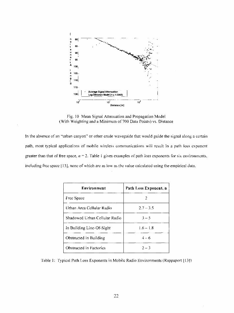
A plot of the average signal attenuation data and the Log-distance Path Loss Model as a function of

distance and the path loss exponent n = 1.0269, as determined using this weighting technique is shown in

Fig. 10. The model appears to be an excellent fit to the average signal attenuation data points over the

range of distances from 8 - 8.0 meters as was expected.

21

[

on80I

it 85 ~

u 90 ~

et 95~tA 100~

a 105

$ ~115~

120i ~ Average Signal AttenuationLog-Distance Model (~ = 1.0269)

100 10~ 102Distance Ira]

Fig. 10 Mean Signal Attenuation and Propagation Model(With Weighting and a Minimum of 700 Data Points) vs. Distance

In the absence of an "urban canyon" or other crude waveguide that would guide the signal along a certain

path, most typical applications of mobile wireless communications will result in a path loss exponent

greater than that of free space, n = 2. Table 1 gives examples of path loss exponents for six environments,

including free space [13], none of which are as low as the value calculated using the empirical data.

Environment Path Loss Exponent, n

Free Space 2

Urban Area Cellular Radio 2.7 - 3.5

Shadowed Urban Cellular Radio 3 - 5

In Building Line-Of-Sight 1.6 - 1.8

Obstructed in Building 4- 6

Obstructed in Factories 2- 3

Table 1" Typical Path Loss Exponents in ]Mobile Radio Environments (Rappaport [13])

22

X. Zhao, et al. used the same Log-Distance Path Loss Model (6) to characterize wideband outdoor mobile

communications signal propagation at 5.3 GHz and found that the path loss exponent was approximately

n = 2.5 in line-of-sight scenarios and n = 3.4 in non-line-of-sight scenarios in suburban environments [4].

Likewise, T. Schwengler and M. Gilbert found that he path loss exponent was approximately n = 2.0 in

line-of-sight scenarios and n = 3.5 in non-line-of-sight scenarios using 5.8 GHz in residential

neighborhoods [5].

In line-of-sight scenarios in urban environments, X. Zhao, et al. did find the path loss to be as low as n =

1.4 [4], however, as stated earlier, the data presented in this thesis was collected in residential suburban

environments characterized by one or two story buildings and residential streets, all of which are

relatively wide-open areas with very limited capability to "confine" the signals to the path taken by the

vehicles. Taking into account that fact that line-of-sight transmissions were at least partially blocked in

many situations, the path loss exponent ofn = 1.0269 is puzzling since all theoretical calculations indicate

that the path loss exponent should be at the very least n = 2 or more likely closer to n = 3.

C.3 Effects of Data Point Distribution "Clipping" on Data Analysis Results’

In an effort to understand the unusually low path loss exponent, the distribution of the signal attenuation

data points was evaluated at ’various distances between the transmitting and receiving nodes.

The distribution of signal attenuation data points for any given distance was determined using the

following technique. First, all packets transmitted from Radio Test Kit A and received by Radio Test Kit

B within a given data set were combined with all packets iransmitted from Radio Test Kit B and received

by Radio Test Kit A within the same data set, forming an aggregate data matrix accounting for two-way

packet transmission between the two radio test kits. Second, a distance "bin" was defined as the one meter

interval centered about the user specified distance with half meter spacing to either side. A search was

then conducted of all packets in the given data ~natrix, identifying all data packets transmitted over a

distance within the distance bin. Third, the maximum and minimum signal attenuation values were

determined and specified a’~; the limits of the range of signal attenuation values at which packets were

received. This range of signal attenuation values was then divided up into one dB segments corresponding

with integer signal attenuation values with a half dB margin to either side, forming a signal attenuation

bin. Fourth, a count was made of all data packets within the distance bin described above whose received

signal had experienced a signal attenuation whose value was within each of the given signal attenuation

bins. Fifth, the total number’ of packets received with each signal attenuation value at the given distance

for each transmitter-receiver pair were summed together one attenuation increment at a time, forming the

total distribution of signal attenuation data points at that given distance for the given individual data set.

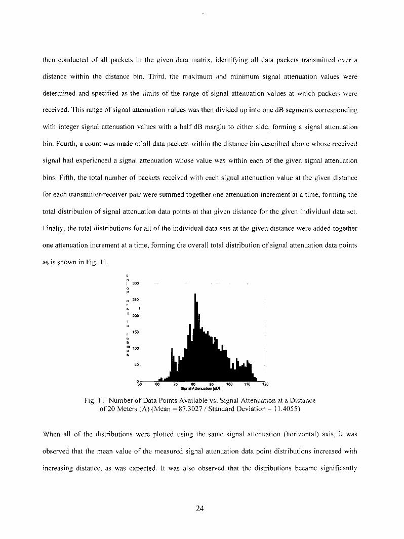
Finally, the total distributions for all of the individual data sets at the given distance were added together

one attenuation increment at a time, forming the overall total distribution of signal attenuation data points

as is shown in Fig. 11.

ni 300 --o

a 250

D 20~

o

~50r

bIn 100uN

5O

60 70 80 90 100 110 120Signal Attenuation1 [dB]

Fig. l I Number of Data Points Available vs. Signal Attenuation at a Distanceof 20 Meters (A) (Mean = 87.3027 / Standard Deviation = 11.4055)

When all of the distributions were plotted using the same signal attenuation (horizontal) axis, it was

observed that the mean value of the measured signal attenuation data point distributions increased with

increasing distance, as was expected. It was also observed that the distributions became significantly

24

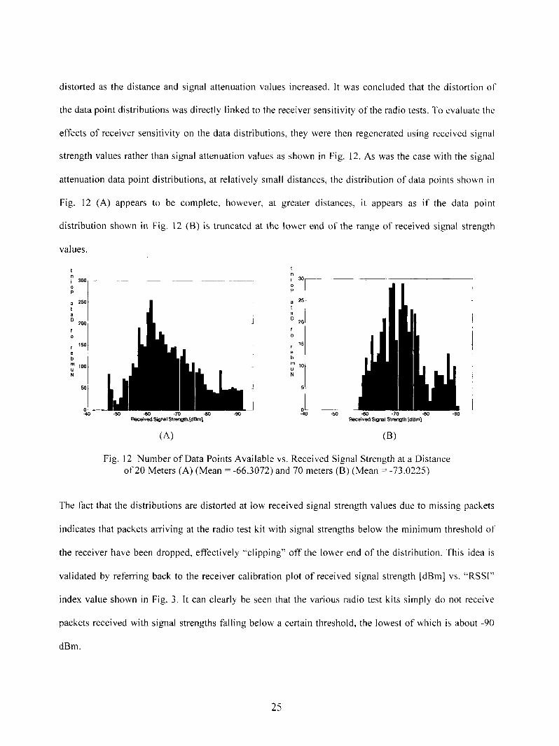
distorted as the distance and signal attenuation wLlues increased. It was concluded that the distortion of

the data point distributions was directly linked to the receiver sensitivity of the radio tests. To evaluate the

effects of receiver sensitivity on the data distributions, they were then regenerated using received signal

strength values rather than signal attenuation values as shown in Fig. 12. As was the case with the signal

attenuation data point distributions, at relatively small distances, the distribution of data points shown in

Fig. 12 (A) appears to be complete, however, at greater distances, it appears as if the data point

distribution shown in Fig. 12 (B) is truncated at the lower end of the range of received signal strength

values.

t

300 [oP

250 a 25ta

i ~20(] 20

f0

150 ~ 15re

~i b

100 ~m 10uN

0-40 -50 -60 -70 -80 -90 -40 -50 -60 -70 -80

Received Signat Strength [dE]m] Received Signal Strength [dBrn]

(A) (B)

-9O

Fig. 12 Number of Data Points Available vs. Received Signal Strength at a Distanceof 20 Meters (A) (Mean = -66.3072) and 70 meters (B) (Mean = -73.0225)

The fact that the distributions are distorted at low received signal strength values due to missing packets

indicates that packets arriving at the radio test kit with signal strengths below the minimum threshold of

the receiver have been dropped, effectively "clipping" off the lower end of the distribution. This idea is

validated by referring back to the receiver calibration plot of received signal strength [dBm] vs. "RSSI"

index value shown in Fig. 3. It can clearly be seen that the various radio test kits simply do not receive

packets received with signal strengths falling below a certain threshold, the lowest of which is about -90

dBm.

25

If the portion of the distribution corresponding to lower signal attenuation values is missing data points,

the mean value of the distribution will be artificially raised. Artificially high mean signal attenuation

values would cause the slope of the regression line to be artificially shallow, effectively decreasing the

calculated value of the path loss exponent.

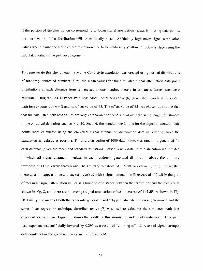
To demonstrate this phenomenon, a Monte-Carlo style simulation was created using normal distributions

of randomly generated numbers. First, the mean values for the simulated signal attenuation data point

distributions at each distance from ten meters to one hundred meters in ten meter increments were

calculated using the Log-Distance Path Loss Model described above (6), given the theoretical free-space

path loss exponent of n = 2 and an offset value of 65. The offset value of 65 was chosen due to the fact

that the calculated path loss values are very comparable to those shown over the same range of distances

in the empirical data plots such as Fig. 10. Second, the standard deviations for the signal attenuation data

points were calculated using the empirical signal attenuation distribution data in order to make the

simulation as realistic as possible. Third, a distribution of 5000 data points was randomly generated for

each distance, given the mean and standard deviations. Fourth, a new data point distribution was created

in which all signal attenuation values in each randomly generated distribution above the arbitrary

threshold of 115 dB were thrown out. The arbitrary threshold of 115 dB was chosen due to the fact that

there does not appear to be any packets received with a signal attenuation in excess of 115 dB in the plot

of measured signal attenuation values as a function of distance between the transmitter and the receiver as

shown in Fig. 8, and there are no average signal attenuation values in excess of 115 dB as shown in Fig.

10. Finally, the mean of botl~t the randomly generated and "clipped" distributions was determined and the

same linear regression technique described above (7) was used to calculate the simulated path loss

exponent for each case. Figure 13 shows the results of this simulation and clearly indicates that the path

loss exponent was artificially lowered by 0.291 as a result of "clipping off" all received signal strength

data points below the given receiver sensitivity threshold.

26

Average ValueLinear Regr ( n = 2.0034)Clip Average ValueClip Linear Regr (n = 1.7124)

[

n 80 ~--~

oit

une 90 i

g 100

S

10~ 102

Distance [m]

Filg. 13 Average Values and Linear Regression Linevs. Distance for Monte-Carlo Simulation

Techniques such as the Expectation Maximization (EM) Algorithm [14,15] make it possible

mathematically fill in the missing portion of a data point distribution if the type of distribution is known.

Although this simulation demonstrates that incomplete data point distributions introduce significant error

into the simulated path loss exponent calculation, the amount of error determined by the simulation does

not account for the entirety of the error in the path loss exponent calculation of the empirical data.

C.4 Determination of Standard Deviation of Gaussian Random Variable

As previously stated, a plot of all signal attenuation data points vs. distance between transmitter and

receiver shows that there is a distribution of signal attenuation data points at each distance. The Log-

Normal Path Loss Model (5) accounts for these data point distributions by including the zero-mean

Gaussian distributed random variable, Xo, with standard deviation, ~.

The standard deviation, ~, of the zero-mean Gaussian distributed random variable, X~, was determined in

the following way. First, all of the fast-fading effects were removed from the data using the time

averaging technique described above. This is important due to the fact that only the large-scale fading

27

effects can be accurately modeled using a Gaussian distribution - the fast-fading effects yield different

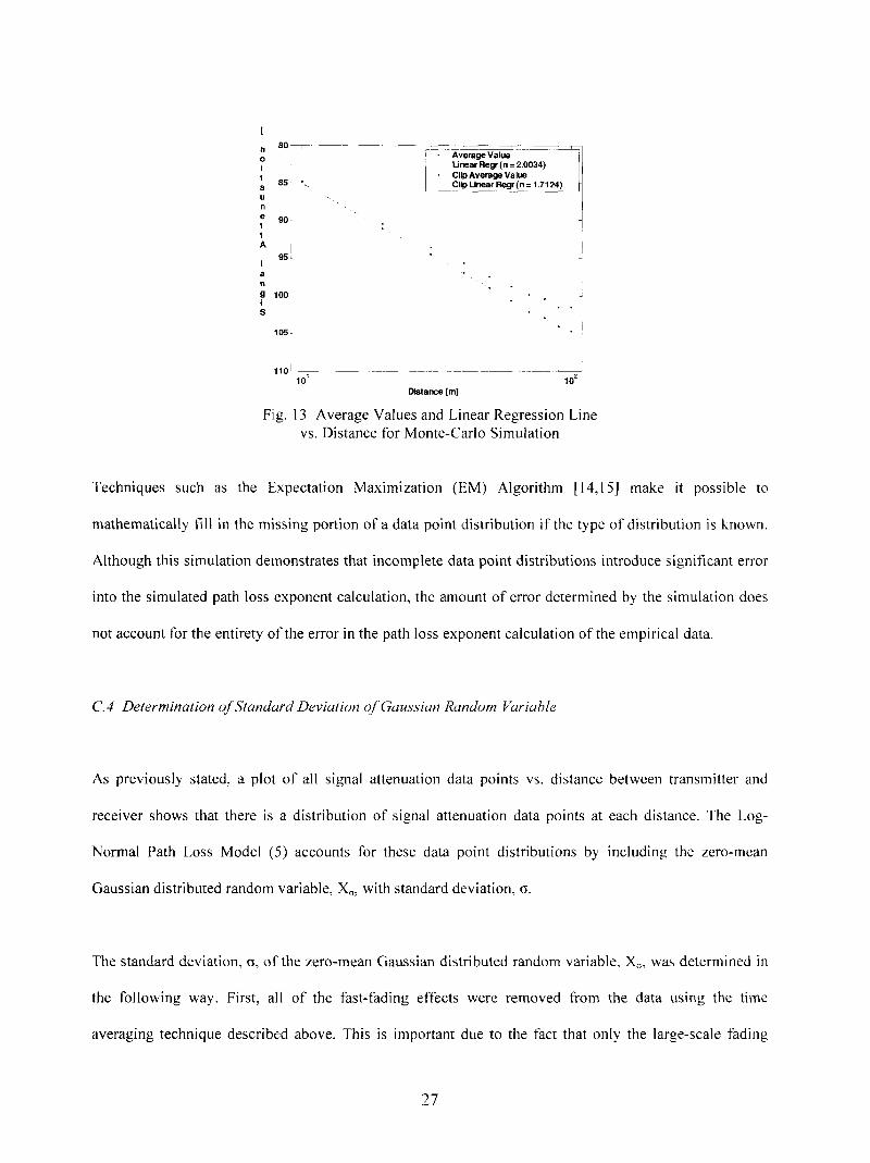
types of distributions not included in the Log-Normal Path Loss Model. Second, all signal attenuation

data points in which both the transmitter and the receiver were stationary (zero velocity) were discarded.

This was necessary due to the fact that the distributions have large spikes at attenuation levels

corresponding to the distances of separation between stationary vehicles. The distribution of data points

shown in Fig. 14 was created using the same set of data points used to create the distribution of data

points shown in Fig. l I above, however, the time averaging technique was used to remove the last-fading

effects and all data points corresponding to stationary vehicles were removed. Note that the large spike at

about 82 dB of attenuation has been removed and the irregular bump at about 110 dB has been smoothed

out.

n

oi 180IP 160~

at ~4oL

fo 100~

b

N

050 60 70 80 90 100 110 120

S~gnal Attenuation [dB]

Fig. 14 Number of Time Averaged Data Points AvailableCorresponding to Vehicles in Motion vs. Signal Attenuation at a Distance

of 20 Meters (A) (Mean = 87.0275 / Standard Deviation = 9.5449)

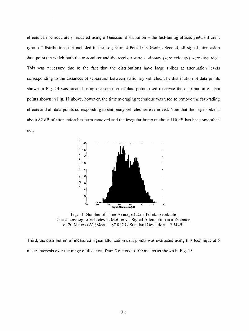
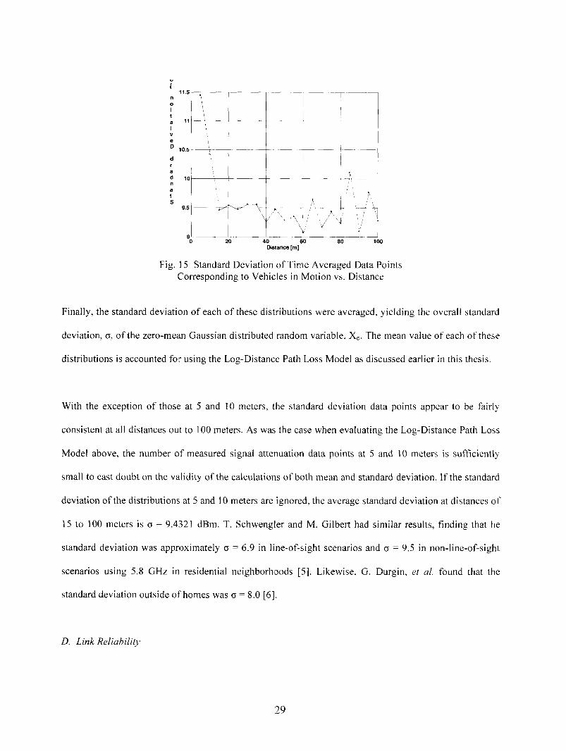
Third, the distribution of measured signal attenuation data points was evaluated using this technique at 5

meter intervals over the range of distances from 5 meters to 100 meters as shown in Fig. 15.

11.5

o

1a 11

v

D 10.5

d

9.5

9 ~0 20 40 60 80 100

D~st a nce [m]

Fig. 15 Standard Deviation of Time Averaged Data PointsCorresponding to Vehicles in Motion vs. Distance

Finally, the standard deviation of each of these distributions were averaged, yielding the overall standard

deviation, ¢~, of the zero-mean Gaussian distributed random variable, Xo. The mean value of each of these

distributions is accounted for using the Log-Distance Path Loss Model as discussed earlier in this thesis.

With the exception of those at 5 and l0 meters, the standard deviation data points appear to be fairly

consistent at all distances out to 100 meters. As wa,.s the case when evaluating the Log-Distance Path Loss

Model above, the number of measured signal attenuation data points at 5 and 10 meters is sufficiently

small to cast doubt on the validity of the calculations of both mean and standard deviation. If the standard

deviation of the distributions at 5 and 10 meters are ignored, the average standard deviation at distances of

15 to 100 meters is c~ = 9.4321 dBm. T. Schwengler and M. Gilbert had similar results, finding that he

standard deviation was approximately ~ = 6.9 in line-of-sight scenarios and c~ = 9.5 in non-line-of-sight

scenarios using 5.8 GHz in residential neighborhoods [5]. Likewise, G. Durgin, et al. found that the

standard deviation outside of homes was ~ = 8.0 [6].

D. Link Reliability

29

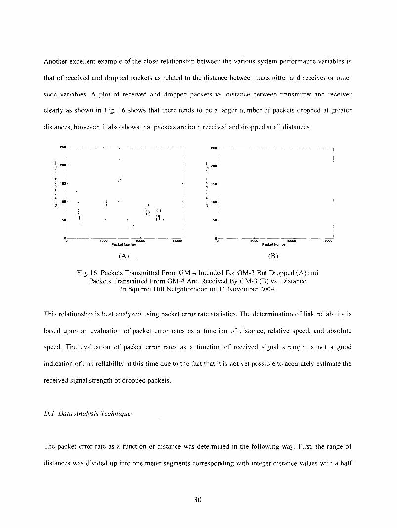
Another excellent example of the close relationship between the various system performance variables is

that of received and dropped packets as related to the distance between transmitter and receiver or other

such variables. A plot of received and dropped packets vs. distance between transmitter and receiver

clearly as shown in Fig. 16 shows that there tends to be a larger number of packets dropped at greater

distances, however, it also shows that packets are both received and dropped at all distances.

m 20~

c 1~n

~taD 100

C I~0 ~

t

5000 10000 15000 0 5000 10000 15000Packet Rlurnber Packet Number

(A) (B)

Fig. 16 Packets Transmitted From GM--4 Intended For GM-3 But Dropped (A) andPackets Transmitted From GM-4 And Received By GM-3 (B) vs. Distance

in Squirrel Hill Neighborhood on 11 November 2004

This relationship is best analyzed using packet error rate statistics. The determination of link reliability is

based upon an evaluation of packet error rates as a function of distance, relative speed, and absolute

speed. The evaluation of packet error rates as a function of received signal strength is not a good

indication of link reliability at this time due to the fact that it is nol yet possible to accurately estimate the

received signal strength of dropped packets.

D. 1 Data Analysis Techniques

The packet error rate as a function of distance was determined in the following way. First, the range of’

distances was divided up into one meter segments corresponding with integer distance values with a halt"

.30

meter margin to either side, forming a "bin." Second, a count was made of all data packets that ’were

received while the nodes were at a distance within the given bin. Third, a similar count was made o,f all

data packets that were dropped at a distance within the given bin. Finally, the packet error rate (PER) was

calculated for each distance by dividing the number of packets dropped by the total number of packets

sent(8).

num_ dropPER = (8)nurn _ drop + num_ rec’ d

A very similar technique was used to determine the packet error rate as a function of absolute and relative

speeds, dividing the range of speeds into a series of bins and counting the number of packets received and

dropped at each speed interval.

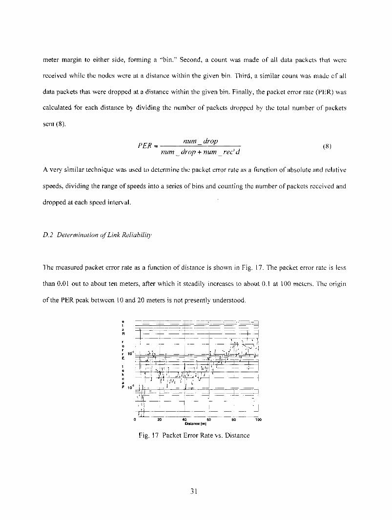
D.2 Determination of Link Reliabili~

The measured packet error rate as a function of distance is shown in Fig. 17. The packet error rate is less

than 0.01 out to about ten meters, after which it steadily increases to about 0.1 at 100 meters. The origin

of the PER peak between 10 and 20 meters is not presently understood.

10-2

0 20 40 60 80 1 O0D~stance [m]

Fig. 17 Packet Error Rate vs. Distance

.31

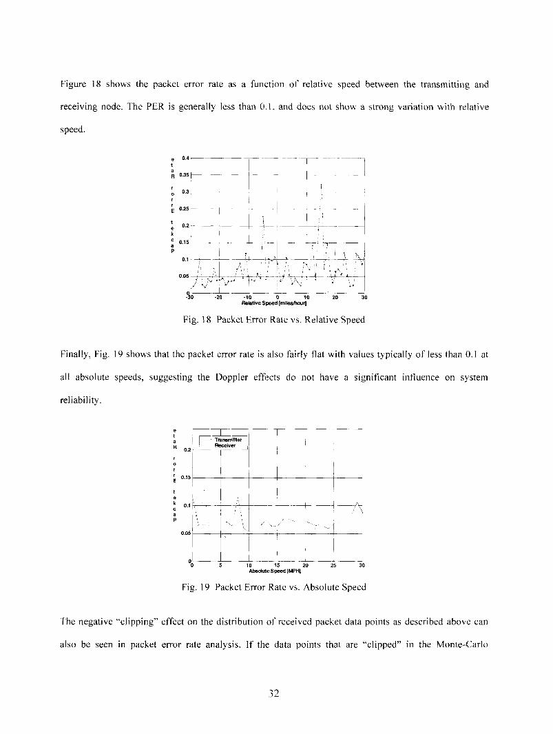
Figure 18 shows the packet error rate as a function of relative speed between the transmitting and

receiving node. The PER is generally less than ().1, and does not show a strong variation with re|ative

speed.

0.05

-20 -1O 0 10 20 30Relative Speed [mileeJhour]

Fig. 18 Packet Error Rate vs. Relative Speed

Finally, Fig. 19 shows that the packet error rate is also thirly flat with values typically of less than 0.1 at

all absolute speeds, suggesting the Doppler effiects do not have a significant influence on system

reliability.

0.2-~

0.15

o.1

01)5

0 5 10 15 20 25 30Absolute Speed [MPH]

Fig. 19 Packet Error Rate vs. Absolute Speed

The negative "clipping" effect on the distribution of received packet data points as described above can

also be seen in packet error rate analysis. If the data points that are "clipped" in the Monte-Carlo

32

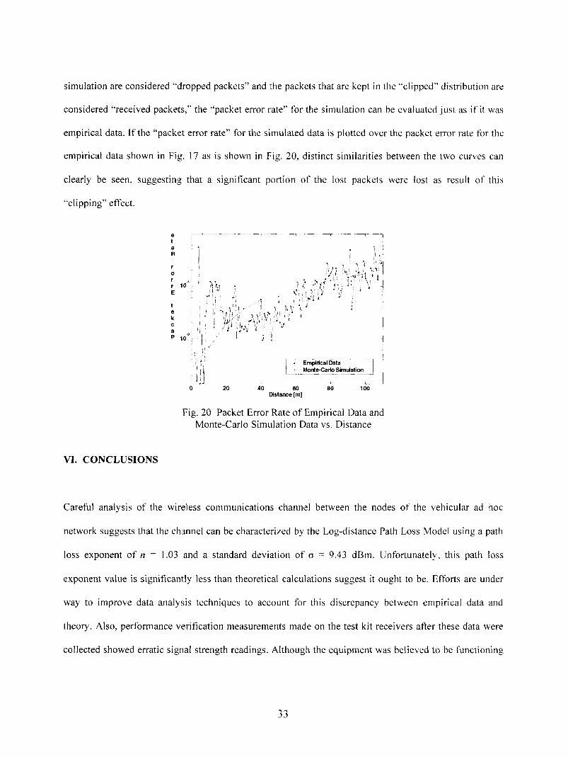
simulation are considered "dropped packets" and the packets that are kept in the "clipped" distribution are

considered "received packets," the "packet error rate" for the simulation can be evaluated just as if it was

empirical data. If the "packet error rate" for the simulated data is plotted over the packet error rate for the

empirical data shown in Fig. 17 as is shown in Fig. 20, distinct similarities between the two curves can

clearly be seen, suggesting that a significant portion of the lost packets were lost as result of this

"clipping" effect.

rorr 10"~

t

p 10=

Empidcal Data -

Monte-Carto Simulation

2~0 40 60 80 1 O0Distance [m]

Fig. 20 Packet Error Rate of Empirical Data andMonte-Carlo Simulation Data vs. Distance

VI. CONCLUSIONS

Careful analysis of the wireless communications channel between the nodes of the vehicular ad hoc

network suggests that the channel can be characterized by the Log-distance Path Loss Model using a path

loss exponent of n = 1.03 and a standard deviation of cy = 9.43 dBm. Unfortunately, this path loss

exponent value is significantly less than theoretical calculations suggest it ought to be. Efforts are under

way to improve data analysis techniques to account for this discrepancy between empirical data and

theory. Also, performance verification measurements made on the test kit receivers after these data were

collected showed erratic signal strength readings. Although the equipment was believed to be functioning

33

correctly during the course of these measurements, equipment malfunction cannot be eliminated as a

possibility at this time.

The evaluation of the packet error rates of the individual links suggests that such links are about 90%

reliable at speeds less than 48 KPH (30 MPH) and distances not in excess of 100 meters in residential

suburban neighborhoods. Figs. 18 and 19 further suggest that there are not any significant Doppler effects

on the packet error rates. The acceptability of the packet error rates is best defined by the tolerance of the

given application.

VII. FUTURE WORK

In spite of the fact that the channel characterization findings were negative, they provide a firm

foundation for future research work. The hardware used in these experiments is no longer in use and new

hardware has been provided to continue the research effort. Once the new hardware is integrated into the

experimental platform, it can be calibrated just as described above, and all of the data analysis tools and

techniques developed and used during this research effort can be used again for future work. If the new

hardware configuration produces similar results, additional work must be done to refine the data analysis

techniques, including careful assessment of the data point averaging techniques, the linear regression

tools, and the weighting of the data points.

One of the challenges that ought to be addressed in the future is the observation that packets transmitted

over greater distances are much less likely to be received, thus creating a much smaller sample size of

received packets at these distances. Additional data ought to be collected at or near the observed

transmission distance limits to increase the size of the data sample, thus increasing the confidence in the

channel characterization and link performance determinations at greater distances. Additional

experiments could be run in which the lost packets are identified and associated with the worst-case SNR

and RSSI values. In such a case, the path loss exponent derived from this experiment would likely serve

as an "upper bound" rather than an absolute value as determined in this thesis.

In addition, future work ought to include the evaluation of various baseline cases in controlled

environments. For example, similar data measurements ought to be taken between vehicles at constant,

known distances and speeds in static and uncluttered environments. A careful evaluation of the channel

characterization and link performance in these "ideal" conditions can then be used as a baseline for

comparison with the unpredictable, dynamic, and cluttered environments common to suburban driving

conditions. Any major variations from this baseline would likely correspond to unique characteristics of

the given suburban driving environment and may explain the findings of this thesis.

35

REFERENCES

[1] R. Mangharam, J. Meyers, R. Rajkumar, D. Stancil, J. Parikh, H. Krishnan, and C. Kellum, "A Multi-hop Mobile Networking Test-bed for Telematics," SAE International, 2005.

[2] K.A. Redmill, M.P. Fitz, S. Nakabayashi, T. Ohyama, F. Ozguner, U. Ozguner, O. Takeshita, K.Tokuda, and W. Zhu, "An Incident Warning System with Dual Frequency Communications Capability,"IEEE Intelligent Vehicles Symposium Proceedings, pp. 552 - 556, 2003.

[3] J. Maurer, T. F/igen, and W. Wiesbeck, "Narrow-Band Measurement and Analysis of the Inter-Vehicle Transmission Channel at 5.2 GHz," 55th IEEE Vehicular Technology Conference Proceedings’,pp. 1274 - 1278, Spring 2002.

[4] X. Zhao, J. Kivinen, P. Vainikainen, and K. Skog, "Propagation Characteristics for WidebandOutdoor Mobile Communications at 5.3 GHz," lEEk," Journal on Selected Areas in Communications, Vol.20, No. 3, April 2002.

[5] T. Schwengler and M. Gilbert, "Propagation Models at 5.8 GHz - Path Loss & Building Penetration,"IEEE Radio and Wireless Conference (RA WCON) 2000 Proceedings, Denver, CO, September 2000.

[6] G. Durgin, T. Rappaport, and H. Xu, "Measurements and Models for Radio Path Loss andPenetration Loss In and Around Homes and Trees at 5.85 GHz," IEEE Transactions on Communications,Vol. 46, No. 11, November 1998.

[7] A. Visser, H. H. Yakali, A-J. van der Wees, M. Oud, G.A. van der Spek, and L.O. Hertzberger, "AHierarchical View on Modeling the Reliability’ of a DSRC Link for ETC Applications," IEEETransactions on Intelligent Transportation Systems, Vol. 3, No. 2, June 2002.

[8] M. Torrent-Moreno, D..liang, and H, Hartenstein, "Broadcast Reception Rates and Effects of PriorityAccess in 802.1 l-Based Velhicular Ad-Hoc Networks," International Conference on Mobile Computingand Networking - Proceedings of the First ACM Workshop on Vehicular Ad Hoc Networks’, pp. 10 - 18,Philadelphia, PA, October 2004.

[9] J. Yin, T. E1Batt, G. Yeung, B. Ryu, S. Habermas, H. Krishnan, and T. Talty, "PerformanceEvaluation of Safety Applications over DSRC Vehicular Ad Hoc Networks," International Conference’ onMobile Computing and Networking - Proceedings of the First ACM Workshop on Vehicular Ad HocNetworks’, pp. 1 - 9, Philadelphia, PA, October 2004.

[10] C.E. Perkins and E.M lVloyer, "Ad Hoc On-Demand Distance Vector Routing," Proceedings of the2~d IEEE Workshop on Mobile Computing Systems" and Applications, pp. 90-100, New Orleans, LA,

February 1999.

[ll] U.S. Census Bureau Geographical Systems FAQ, "Q5.1: What is the best way to calculate thedistance between 2 points?," http://www.census.~ov/c~i-bin/~eo/jzisfiaq?Q5.1, 2001.

[12] D.C. Cox, R.R. Murray, A.W. Norris, "800 MHz Attenuation Measured in and around SuburbanHouses," A T& T Bell Labs l’echnical Journal, Vol. 63, pp. 921-954, July/August 1984.

36

[| 3] Rappaport, Theodore S., Wireless Communications" Principles and Practice, 2nd ed., Upper SaddleRiver, NJ: Prentice Hall PTR, 2002.

[14] A. Dempster, N. Laird, and D. Rubin, "Maximum likelihood from incomplete data via the EMalgorithm," Journal of the Royal Statistical Society, Series B, 39(1), pp. 1-38, 1977.

[15] G. McLachlan, and T. Krishnan, The EMAlgorithm and Extensions, New York: John Wiley & Sons,Inc., 1997.

37

APPENDIX A

Transmitter Calibration Techniques

Before the transmission power could be calibrated, Daniel Weller had to write a special "TXTest"

program which allowed the.. user to easily change the "ForcePower" settings, reinitialize the network,

transmit packets from the transmitting radio test kit to the receiving radio test kit for a specified period of

time, and then repeat the process for the full range of power settings.

The power [dBm] transmitted at a given "ForcePower" setting for the various radio test kits was

calibrated using the following technique. First, a radio test kit other than the one whose transmission

power was to be calibrated was selected to serve as the "server" radio test kit (receiver) and M/A-Com

ground-plane mount 802.1 l a radio antenna was connected to the antenna port. Second, the GTK

RoadMap program was started up on the receiver radio test kit to initialize the radio card, after which the

RoadMap graphical user interface was closed and IPERF Version 1.7.0 was started up to coordinate

packet transmission over the wireless communications link with the transmitting radio test kit. Third, a

Pomona Electronics BNC-C-36 Alpha Wire-J P/N 9058C RG 58C/U cable, in series with a Hewlett

Packard 8473C (0.01-26.5 GHz STD) Detector (Serial 1822A: 03039) and a RLC Electronics A-41-10-R

10 dB attenuator (8521), was used to link a Hewlett Packard 54645D (100 MHz 2+16 channel) Mixed

Signal Oscilloscope to the antenna port of the "client" radio test kit whose transmission power was to be

calibrated as shown in Fig. A-I. The antenna from the receiver test kit was then placed near the radio card

of the radio test kit whose transmission power was being calibrated to capture the signal leakage and

complete the wireless communications link between the two test kits. Fourth, the client (transmitter) and

server (receiver) IP addresses were specified in the TXTest program script. Fifth, the starting and ending

"ForcePower" values were specified as the TXTest program was started up on the transmitter radio test

kit, creating a transmitted packet signal waveform on the oscilloscope screen. Sixth, the time (horizontal)

38

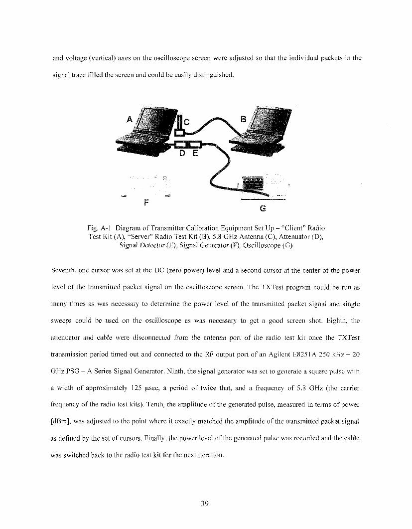
and voltage (vertical) axes on the oscilloscope screen were adjusted so that the individual packets in the

signal trace filled the screen and could be easily distinguished.

Fig. A-1 Diagram of Transmitter Calibration Equipment Set Up - "Client’" RadioTest Kit (A), "Server" Radio Test Kit (B), 5.8 GHz Antenna (C), Attenuator

Signal Detector (E), Signal Generator (F), Oscilloscope

Seventh, one cursor was set at the DC (zero power) level and a second cursor at the center of the power

level of the transmitted packet signal on the oscilloscope screen. The TXTest program could be run as

many times as was necessary to determine the power level of the transmitted packet signal and single

sweeps could be used on the oscilloscope as was necessary to get a good screen shot. Eighth, the

attenuator and cable were disconnected from the antenna port of the radio test kit once the TXTest

transmission period timed out and connected to the RF output port of an Agilent E8251A 250 kHz- 20

GHz PSG - A Series Signal Generator. Ninth, the signal generator was set to generate a square pulse with

a width of approximately 125 gsec, a period of twice that, and a frequency of 5.:8 GHz (the carrier

frequency of the radio test kits). Tenth, the amplitude of the generated pulse, measured in terms of power

[dBm], was adjusted to the point where it exactly matched the amplitude of the transmitted packet signal

as defined by the set of cursors. Finally, the power level of the generated pulse was recorded and the cable

was switched back to the radio test kit for the next iteration.

39

This procedure was repeated once for each "ForcePower" index value, creating a single calibration data

set. After taking five complete calibration data sets, the measured power values [dBm] for each

"ForcePower" index value were averaged, yielding a calibration table of "ForcePower" index values and

the corresponding as overall average power values [dBm] shown graphically in Fig. 2.

40

APPENDIX B

Receiver Calibration Techniques

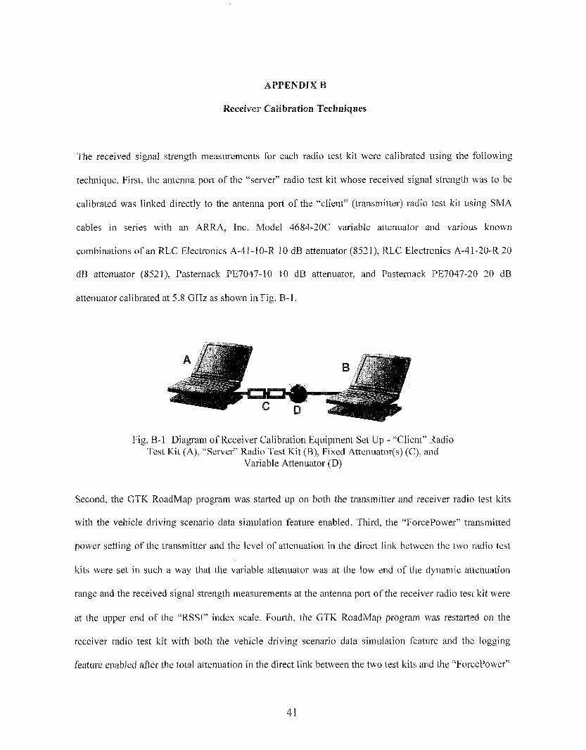
The received signal strength measurements for each radio test kit were calibrated using the following

technique. First, the antenna port of the "server" radio test kit whose received signal streng*h was to be

calibrated was linked directly to the antenna port of the "client" (transmitter) radio test kit using SMA

cables in series with an ARRA, Inc. Model 4684-20C variable attenuator and various known

combinations of an RLC Electronics A-41-10-R 10 dB attenuator (8521 ), RLC Electronics A-41-20-R

dB attenuator (8521), Pasternack PE7047-10 10 dB attenuator, and Pasternack PE7047-20 20

attenuator calibrated at 5.8 GHz as shown in Fig. B-1.

A

Fig. B-1 Diagram of Receiver Calibration Equipment Set Up - "Client" RadioTest Kit (A), "Server" Radio Test Kit (B), Fixed Attenuator(s) (C),

Variable Attenuator (D)

Second, the GTK RoadMap program was started up on both the transmitter and receiver radio test kits

with the vehicle driving scenario data simulation feature enabled. Third, the ’°ForcePower" transmitted

power setting of the transmitter and the level of attenuation in the direct link between the two radio test

kits were set in such a way that the variable attenuator was at the low end of the dynamic attenuation

range and the received signal strength measurements at the antenna port of the receiver radio test kit were

at the upper end of the "RSSI" index scale. Fourth, the GTK RoadMap program was restarted on the

receiver radio test kit with both the vehicle driving scenario data simulation feature and the logging

feature enabled after the total attenuation in the direct link between the two test kits and the ~’ForcePower"

41

transmission power index of the transmitter were. manually recorded. Fifth, the transmission of packets

from transmitter and receiw~r radio test kits was started by activating the client function on the transmitter

and the server function on the receiver. Sixth, the transmission of packets from transmitter and receiver

radio test kits was stopped by deactivating the server function on the receiver after running for

approximately forty-five seconds. Seventh, the attenuation of the variable attenuator was increased by one

increment and the transmission of packets from transmitter and receiver radio test kits was restarted (no

less than twenty seconds after being stopped) by reactivating the server function on the receiver,

beginning the next iteration of logged measurements.

This procedure was repeated until the variable attenuator reached the upper end of its dynamic attenuation

range. At this point, the log file was saved, the transmitted "ForcePower" power setting and level of

attenuation in the direct link between radio test kits were set to levels which resulted in "RSSI" values at

or just slightly above the level last measured, the new transmission power and attenuation levels were

manually recorded, a new log file was created by restarting the GTK RoadMap program on the receiver

radio test kit with both the vehicle driving scenario data simulation feature and the logging feature

enabled, and the measurement procedure was continued as before. Once the attenuation was increased to

the point that the received signal strength fell below the minimum received signal strength threshold of

the radio card and the radio test kit no longer received data packets, the log was saved and the test kits

were shut down.

The data log files were then downloaded and the following procedure was used to determine the average

received signal strength value corresponding to each "RSSI" index value. First, the two complete data sets

corresponding to the upper and lower halves of the range of"RSSI" index values for each radio test kit

were individually parsed and placed into raw data matrices containing the packet number, the radio test

kit ID number, the time stamp, and the "ForcePower" or "RSSI" index value for each packet. Second, all

data in each raw data matrix corresponding to packets transmitted from that radio test kit was discarded,

leaving only the data corresponding to received packets. Third, each raw data matrix was restructured into

a new data matrix containing the variable attenuator setting and the packet number, radio test kit

number, time stamp, and "RSSI" index value con’esponding to each packet received at the given signal

attenuation level. Fourth, the value of each of the variable attenuator settings was replaced in the new data

matrix with the calibrated attenuation values [dB] corresponding to each setting. Fifth, all packets

corresponding to each of the possible "RSSI" index values were located in the given data matrix.

variable attenuator attenuation values [dB] corresponding to all packets received at each given "RSSF’

index value were averaged, which yielded an array of mean attenuation values for the variable attenuator

corresponding to each "RSSi" index value. This process was repeated for each of the two data sets. Sixth,

the value of the known fixed attenuation for the given data set was added to the array of mean attenuation

values for the variable attenuator for each of the two data sets. Seventh, the array of total attenuation

values [dB] corresponding to each of the "RSSI" index values was subtracted from the known transmitted

power value [dBm], yielding an array of received power values [dBm]. Finally, the two data sets of date

were combined together, yielding a calibration table of "RSSI" index values and the corresponding

received signal strength for each as shown graphically in Fig. 3. In the cases where the data contained

within the two data sets overlapped, an average value for the received signal strength was calculated by

summing the product of the received signal strength value and the number of data points used to

calculated that value for the given "RSSI" index value in each of the two data sets and dividing it by the

sum of number of data point’s used to calculated the received signal strength values for the given "RSSI"

index value in both of the data sets.

43