Changing Progressivity as a Means of Risk … Progressivity as a Means of Risk Protection in Investment-Based Social Security Andrew A. Samwick NBER Working Paper No. 13059 April 2007

NBER WORKING PAPER SERIES

CHANGING PROGRESSIVITY AS A MEANS OF RISK PROTECTION IN INVESTMENT-BASEDSOCIAL SECURITY

Andrew A. Samwick

Working Paper 13059http://www.nber.org/papers/w13059

NATIONAL BUREAU OF ECONOMIC RESEARCH1050 Massachusetts Avenue

Cambridge, MA 02138April 2007

I thank Mike Hurd and conference participants at the NBER Program on Aging's 2006 Conferenceon Retirement Research for helpful comments. This research was supported by the U.S. Social SecurityAdministration through grant #10-P-98363-1-03 to the National Bureau of Economic Research aspart of the SSA Retirement Research Consortium. The findings and conclusions expressed are solelythose of the author and do not represent the views of SSA, any agency of the Federal Government,or the NBER. Any errors are my own.

© 2007 by Andrew A. Samwick. All rights reserved. Short sections of text, not to exceed two paragraphs,may be quoted without explicit permission provided that full credit, including © notice, is given tothe source.

Changing Progressivity as a Means of Risk Protection in Investment-Based Social SecurityAndrew A. SamwickNBER Working Paper No. 13059April 2007JEL No. D31,H55,J26

ABSTRACT

This paper analyzes changes in the progressivity of the Social Security benefit formula as a meansof lessening the risk inherent in investment-based Social Security reform. Focusing on a single cohortof workers, it simulates the distribution of benefits subject to both earnings and financial risks in areformed system in which solvency has been restored and traditional benefits have been augmentedby personal retirement accounts (PRAs). The simulations show that some investment in equities isdesirable in all cases. However, switching from the current benefit formula to the maximally progressiveformula -- a flat benefit independent of earnings -- improves the welfare of the the bottom 30 percentof the earnings distribution even if they reduce their PRA investments in equity to zero. An additional30 percent of earners can lessen their equity investments without loss of welfare under the maximallyprogressive formula. Intermediate approaches in which traditional benefit replacement rates for lowerearnings are reduced by less than those for higher earnings allow about half of the equity risk to beeliminated for the lowest earnings decile. Sensitivity tests show that these patterns are robust to differentassumptions about risk aversion, the equity premium, and the size of the personal retirement accountsestablished by the reform.

Andrew A. Samwick6106 Rockefeller HallDepartment of EconomicsDartmouth CollegeHanover, NH 03755-3514and [email protected]

I. Introduction

Around the globe, traditional pay-as-you-go Social Security systems are facing

financial challenges due to demographic changes. With fertility rates at or below

replacement levels in developed countries and life expectancy in retirement projected to

continue increasing, the ratio of beneficiaries to workers will rise over the coming

decades, increasing annual costs relative to income. The imminent retirement of the

Baby Boom generation in many developed countries has focused attention on the need

for reform.1

Over the past decade and more, many analysts have proposed that at least some of

the financial shortfalls be eliminated through the prefunding of future benefits, in order to

ameliorate the increase in pay-as-you-go tax rates on future generations of workers that

would otherwise be required.2 Prefunding can more readily take place in a system of

decentralized Personal Retirement Accounts (PRAs) than in the Social Security Trust

Fund, particularly when it is desired to exploit the risk-return tradeoff inherent in the

equity premium and to separate the incremental saving due to higher Social Security

taxes from the rest of the federal government’s budget.3

The possibility that Social Security benefits paid from personal accounts would be

subject to financial risk due to stock return volatility, in turn, has focused attention on

ways limit the risk in investment-based Social Security reform. Financial risk is of

particular concern with respect to low-income beneficiaries, for whom Social Security

1 The Social Security Trustees Report 2006 projects an increase in the number of beneficiaries per hundred workers from 30 in 2005 to 49 in 2040 to 53 in 2080 (Table IV.B2). For an international description of the demographic challenge, see World Bank (1994). 2 The Office of the Chief Actuary at the Social Security Administration has formally analyzed over two dozen proposals. See the memoranda at http://www.ssa.gov/OACT/solvency/ . 3 See Samwick (1999, 2004) for further discussion of the role of PRAs in prefunding future entitlement benefits.

2

benefits make up a disproportionate share of their retirement income. Two principal

methods of limiting financial risk have been explored in the recent literature. The first is

to offer a guarantee to workers that benefits will not fall below a particular threshold

(e.g., 90 percent of scheduled benefits). Feldstein and Ranguelova (2001a,b) demonstrate

that such guarantees can be implemented via long-term options on a stock market index

in a manner similar to conventional portfolio insurance. The second method is to follow

popular financial planning strategies that reduce the portfolio allocation in equities as a

worker approaches retirement. Poterba, Rauh, Venti, and Wise (2006) explore the

efficacy of using such “life cycle” strategies in this context.

These two mechanisms share the feature that they introduce bonds (preferably as

inflation-indexed securities) into the portfolio in order to lessen the exposure to equity

risk. However, in doing so, these mechanisms give up the equity premium and thus lose

one very important rationale for including PRAs in the reform. In contrast, the analysis

below considers an alternative approach based on modifications to the traditional benefit

to protect low-earning workers while leaving all workers free to choose their own PRA

portfolios. Such an approach may prove to be useful, particularly because any

restrictions on the portfolio allocations in the PRAs beyond the determination of which

investment choices will be offered are likely to be untenable as the accounts become

larger and more popular.

The most direct way to make sure that low-earning workers do not fall into

poverty in old age is to increase the progressivity of the benefit formula in the scaled-

down version of the traditional system that remains after reform. Doing so would lessen

the need to provide insurance against possibly low returns in the PRAs, because low-

3

income retirees would depend less on the PRAs to stay out of poverty. To be sure, there

have been discussions of progressive reductions in the traditional benefits as part of a

plan to close the financial gap while protecting low-earning workers. This paper adds to

the literature by quantifying the effect of such changes to the traditional benefit formula

on the need to invest PRAs in equity rather than bonds to achieve a given level of

welfare.

This paper illustrates the link between progressivity and risk using a stylized

framework based on simulations of earnings trajectories and portfolio returns. The

simulations are based on the projected experience of a cohort of workers corresponding

roughly to those born in 1973. To calibrate the simulations, traditional retirement

benefits are reduced by 40 percent, an amount comparable to what is projected to be

required to restore annual balance to the system in the long term.4 The simulations pair

reductions in the traditional benefits of this magnitude with PRAs funded by

contributions of 2 percent of covered earnings each year. The main comparisons are

between the utility-maximizing portfolio allocations to equities across the new

configurations of the traditional benefit that are more versus less progressive.

The key finding is that under baseline parameters, the most progressive traditional

benefit—a flat benefit independent of earnings—allows the bottom 30 percent of the

earnings distribution to achieve a higher expected utility than under the proportional

reductions to the current benefit formula even if they reduce their PRA investments in

4 In 2080, the latest year of the projections in the Social Security Trustees Report 2006 (Table IV.B1), the annual gap is 5.38 percentage points of taxable payroll, compared to a cost rate (excluding disability insurance benefits) of 16.27 percentage points of taxable payroll. Thus, the required reduction is 5.38/16.27 = 33 percent. However, this figure assumes that all benefits—including those of current retirees—can be cut by this amount. The need to protect benefits already in payment would lead to a higher cut to benefits yet to be paid.

4

equity to zero. An additional 30 percent of earners can lessen their equity investments to

some degree without loss of welfare relative to those available under the proportionally

scaled-back current formula. Under more realistic and less extreme changes to the

traditional benefit, such as that proposed by Liebman, MacGuineas, and Samwick (2005),

about half of the equity risk can be eliminated for the lowest earnings decile, and some

equity risk can be eliminated for the bottom six deciles. The optimal allocation to

equities in the PRA is not particularly sensitive to the progressivity of the reductions in

the traditional benefits—in most simulations, the share in equities increases slightly for

low earners and decreases slightly for high earners with more progressive reductions in

the traditional benefits.

The remainder of the paper is organized as follows. Section II lays out the

simulation framework for both the traditional benefits and the new system of PRAs.

Section III discusses the combinations of PRA asset allocations and reductions in the

traditional benefits that will be analyzed. Section IV derives the certainty equivalent

measure of expected utility that will be used in the comparisons. Section V presents the

baseline results, and Section VI includes sensitivity tests and a comparison to life cycle

investment strategies. Section VII concludes.

II. The Simulation Framework

The model used in the analysis focuses on a cohort of workers who should expect

to have their traditional benefits reduced at some point when the Social Security system is

restored to solvency. Specifically, the analysis simulates the experience of the birth

cohort of 1973, who will reach their normal retirement age in 2040, just as the Social

5

Security trust fund is presently projected to be exhausted. Trust Fund exhaustion will

necessitate changes to the system, even if they have not been made before that time. The

analysis assumes, counterfactually, that the workers have been in the new system since

they entered the workforce.

The distribution of earnings at an initial age is assumed to be lognormal, allowing

its parameters to be estimated from the mean and median of a sample of data. Kunkel

(1996) reports the mean and quartiles of the distribution of earnings by age group for the

years 1980-1993 based on a detailed sample of Social Security records. The population

of 30 year olds in this analysis is approximated by the 25 – 34 year old cohort in

Kunkel’s data, and parameters of the lognormal are estimated for each year of Kunkel’s

sample.5 These parameters are averaged across all the sample years, and the resulting

distribution is scaled up by the growth in the average wage index in Social Security

through 2003, the last year for which an estimate of that index is currently available in

SSA (2006). To allow for the analysis of the distributional consequences of changes to

the Social Security benefit formula, the lognormal distribution is approximated by ten

workers who fall at the midpoints of the deciles of that distribution.

For each such worker, earnings evolve over the life cycle due to deterministic

changes in expected earnings and stochastic shocks to earnings around expected earnings.

The results of the analyses below are the distributions of simulated benefits, where

simulations are conducted with 5,000 independent replicates for each of the ten workers

representing the deciles of the initial distribution of earnings. The processes for the

5 The median and mean of a lognormal distribution are given by exp(µ) and exp(µ + 0.5*σ2), respectively, where exp( ) denotes the exponential function and µ and σ are the mean and standard deviation of the underlying normal distribution. The median therefore identifies µ and the ratio identifies σ. The estimated parameters for the group discussed in the text are {10.2056, 0.5271}.

6

growth in expected earnings are assumed to be identical for all replicates of all workers.

Expected earnings grow each year due to the growth in the national average wage,

approximated here by the average real growth rate of Social Security covered wages

during the 1952-2003 period, or 1.1 percent per year. Expected earnings also follow an

age-earnings profile, reflecting changes in individual productivity and hours worked over

the life cycle. Each worker is assumed to face the age-earnings profile for the least

educated group of workers analyzed by Hubbard, Skinner, and Zeldes (1994).6

Stochastic deviations from expected earnings follow an AR(1) process with a correlation

coefficient of ρ = 0.95 and a standard deviation of 15 percent.7 Given these parameters,

annual earnings are backcasted from the initial distribution at age 30 (deterministically, at

the average rate of earnings growth) to age 21 and then forecasted to age 67.8

The Social Security benefit formula depends on the growth in the national average

wage in two places: to determine the maximum taxable earnings on which payroll taxes

are paid and to index each year of earnings for the growth of aggregate earnings during a

worker’s career. Since the framework focuses on the deciles of a single age cohort, the

growth in the national average wage is approximated by the growth rate of this cohort’s

average earnings over its career. Maximum taxable earnings subject to the payroll tax are

projected forward and backward from 2003 (age 30) using this growth rate. With these

few assumptions, it is possible to get a reasonable approximation of Social Security

benefits by applying the benefit formula to the simulated earnings profiles. 6 This profile is approximated by having real earnings grow at annual rates of 2.5 percent between ages 21 and 30, 1.7 percent between 31 and 40, 0.5 percent between 41 and 50, and -1.3 percent through age 67. This growth is in addition to the growth in the national average wage. 7 See Topel and Ward (1992) for other, comparable estimates of the wage process. 8 Largely because the sample is constructed around a single deterministic age-earnings profile and is assumed to be fully employed each year, it understates the cross-sectional variation in annual earnings each year. For example, the ratio of the 75th to the 25th percentiles of the earnings distribution at age 50 (or the age group 45-54) in the simulation is 2.59, compared to 3.30 in Kunkel’s (1996) sample.

7

In each of the policy scenarios, the traditional benefit is reduced by 40 percent in

the aggregate and is augmented by the benefits payable from a PRA. PRA contributions

are 2 or 3 percent of earnings (depending on the scenario) up to the maximum taxable

earnings level. Asset returns are based on the annual total returns in Table 2-5 of

Ibboston Associates (2006) for the years 1926 – 2005. Asset classes include large stocks,

small stocks, long-term corporate bonds, long-term government bonds, intermediate-term

government bonds, and Treasury bills. These returns are further combined in to an equity

portfolio (75 percent large stocks and 25 percent small stocks), the corporate bond

portfolio, and a government bond portfolio (one third in each of the long-term,

intermediate-term, and bills). Each age (e.g., 45) in each of the 5,000 replicates is

assigned a random year of returns (e.g., 1973) from this 80-year span. Each of the ten

workers, corresponding to the deciles of the initial distribution of earnings, therefore

receives the same sequence of return-years. Portfolio allocations are as specified for each

scenario. At retirement, PRA balances are converted to inflation-indexed annuities at a

real interest rate of 3 percent, matching the long-term bond return in the Trustees Report.9

III. Combining Personal Accounts with a Smaller Traditional Benefit

Several approaches to reducing traditional pay-as-you-go benefits are considered,

all of which reduce aggregate payouts by 40 percent (because all are designed to restore

solvency to the same degree). They differ in the extent to which they protect the benefits

of low-earners, whose total retirement incomes are more vulnerable to the financial risk

9 The annuity factor is derived from the period life table from 2002, available at http://www.ssa.gov/OACT/STATS/table4c6.html. A dollar of PRA balance translates into $1/13.15 in annual inflation-indexed benefits. The denominator in this figure is the average of the two factors for men (12.3) and women (14.0), respectively.

8

that may come from PRAs. At one extreme is a proportional reduction in the traditional

benefits, in which the entire benefit formula is scaled down by 40 percent. This approach

leaves the progressivity of the traditional benefit unchanged and is referred to as the

Proportional Reduction. At the other extreme, the most progressive way to reduce

traditional benefits is to pay each beneficiary the same amount, regardless of earnings. In

this case, Social Security would play a flat benefit equal to the mean benefit in the system

(scaled down by 40 percent). This method is referred to as the Uniform Benefit below.

Between these two extremes lie other possible approaches. One possibility is to

use a weighted average of the two extremes. The simulations below consider a Half and

Half benefit formula which combines the Proportional Reduction and Uniform Benefit

and then divides the total by two. Another approach is to reduce benefits progressively

based on features of the current benefit formula. For example, in the reform plan

presented by Liebman, MacGuineas, and Samwick (2005), the replacement rates are

lowered by 25 percent below the first bend point in the formula (from 90 to 67.5 percent)

and 50 percent above the first and second bend points (from 32 and 15 percent to 16 and

7.5 percent).10

In a reformed system, PRAs are added to the traditional benefits to help maintain

total retirement replacement rates. The asset allocation decision in PRAs in this

framework is simply a question of equity relative to bonds. The simulations below

consider time-invariant allocations to equity ranging from 0 to 100, effectively assuming

10 See SSA (2006) for a description of the Social Security benefit formula. See Goss and Wade (2005) for an evaluation of the Liebman, MacGuineas, and Samwick (2005) plan. Both documents can be found at http://www.nonpartisanssplan.com for reference.

9

annual rebalancing to meet this allocation target.11 For purposes of comparison, three

“life cycle” strategies are also simulated, in which the allocation to stocks averages 50

percent but declines linearly with age at rates of 1.0, 1.5, or 2.0 percentage points per

year.

When it evaluates Social Security reform plans, the Office of the Chief Actuary at

the Social Security Administration assigns mean returns by asset type. In recent

evaluations, such as Goss and Wade (2005), mean returns have been assumed to be 6.2

percent for equity, 3.2 percent for corporate bonds, and 2.7 for government bonds, net of

both inflation and a modest 30 basis point administrative cost. The baseline simulations

utilize these assumptions. To capture the volatility around the mean, the historical

variation in asset returns from 1926 – 2005 reported by Ibbotson Associates (2006) is

utilized. Standard deviations are 22.2 percent for equity, 9.2 percent for corporate bonds,

and 6.6 percent for government bonds. All simulations preserve these standard

deviations but change the mean returns (by the difference between the specified mean

return and the mean of the historical data), allowing for potentially lower equity

premiums going forward than what SSA’s Office of the Actuary has assumed.12

11 In reality, a worker might choose to vary the allocation to equities over time as a response to realizations of both earnings and investment returns. The assumption of constant allocations throughout the life-cycle greatly simplifies the analysis, in order to focus on the main tradeoff of progressivity in the benefit formula against the need for low-earning workers to exploit the equity premium. The extension to a dynamic programming that solves for the optimal portfolio is a subject for future work. 12 Social Security reform proposals that include PRAs often stipulate that the balance can be bequeathed. Bequests are not modeled in this analysis, but this is not an important omission. Allowing for bequests would simply raise the required contribution rate to the PRA to ensure that the 2 or 3 percentage points specified in the simulations go to fund the annuities.

10

IV. Evaluating Risk in Retirement Benefits

In the main simulations, workers are assumed to have constant relative risk

aversion (CRRA) utility functions, defined over total retirement benefits, b, with risk

aversion coefficient γ:

( )γ

γ

−=

−

1

1bbu

Expected utility for the worker representing each decile of the initial wage

distribution is calculated as the average value of u(b) across 5,000 independently drawn

replicates. It therefore encompasses the uncertainty in both portfolio returns and

earnings, while also allowing for comparisons across different deciles in the initial

earnings distribution.13 As a basis for comparison across configurations of the traditional

benefit formula and the PRA asset allocation rules, we can calculate the certainty

equivalent benefit:

( ) ( )( )[ ] ( ) ( )[ ] ( )γγγγ −−− =−=111111 bEbuEbCE

The certainty equivalent is the retirement benefit that, if received with certainty,

would make the individual equally well off as facing the uncertain benefit distribution.

For a risk averse individual, the certainty equivalent will be less than the expected benefit

level, E(b). A higher certainty equivalent indicates a higher expected utility, and

differences in certainty equivalents correspond to risk premiums measured in dollar

terms.

13 Defining the deciles with respect to initial earnings is appropriate in the current framework in which workers are assumed to adopt a single, time-invariant allocation to equities in their PRAs. An alternative approach to doing distributional analysis would use a measure of average lifetime earnings to assign workers to deciles. For example, some workers in the lowest initial earnings decile receive a number of very positive earnings draws and wind up higher in the distribution of lifetime earnings. For comparison, assigning workers to deciles based on their average indexed monthly earnings yields an allocation to deciles with a correlation of 0.83 with the deciles of the initial earnings distribution.

11

By construction, the aggregate expected benefits from the traditional system are

identical across all policy scenarios, conditional on the earnings realizations. This is not

true within each decile, as some benefit formulas are designed to be more progressive

than others and thus provide differential expected benefits to different deciles. Other

differences in certainty equivalents across the policy scenarios reflect different exposure

to risk, whether through the traditional benefit formula or the PRA investment portfolio,

or different expected benefits through the PRA investment portfolio.

V. Trading off Progressivity and Risk

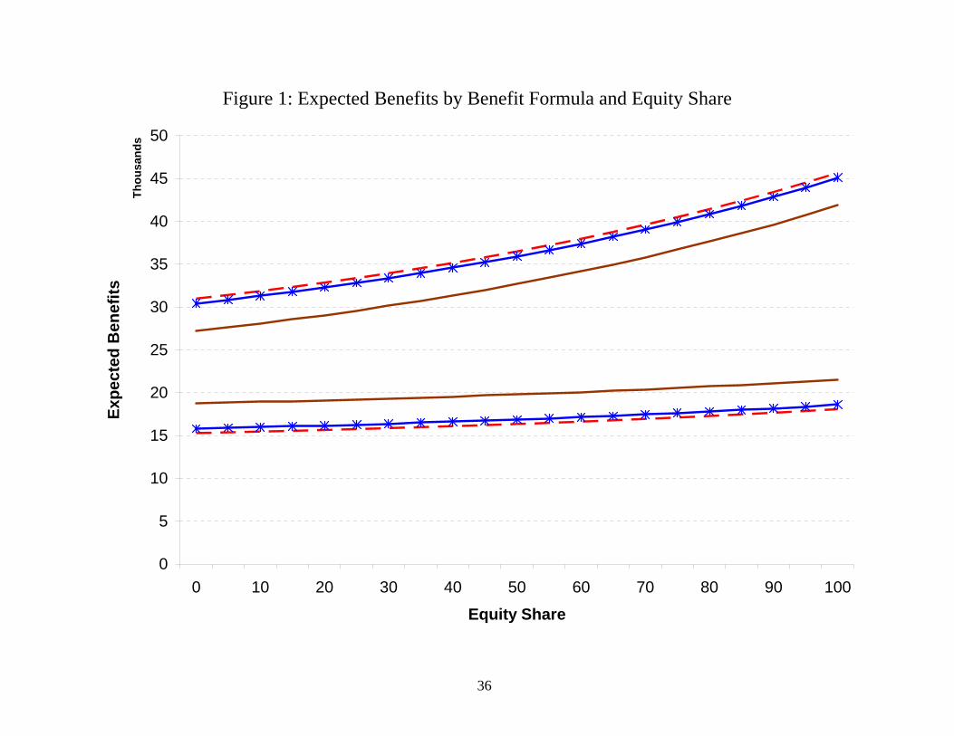
Figure 1 illustrates the impact of the benefit formula and the equity share of the

PRA portfolio on expected benefits. The graph shows the relationship between expected

benefits and the equity share in the PRA portfolio for the highest and lowest earnings

deciles under three different benefit formulas: Proportional Reduction, Progressive, and

Uniform Benefit. The curves for the top decile earner go in that order, and the curves for

the bottom decile go in the reverse order. The Proportional Reduction is most generous

for the top decile and least generous for the bottom decile. The Uniform Benefit is the

opposite—most generous for the bottom decile and least generous for the top decile. The

Progressive benefit reduction actually tracks the Proportional Reduction fairly closely.

The Half and Half benefit formula (not shown) would fall exactly between the

Proportional Reduction and Uniform Benefit.14 Because the risk premium on equities is

positive, expected benefits increase in all cases with the portfolio share in equities. For

14 For the bottom decile, the reductions in the average traditional benefit relative to current law are 40, 37.6, 32.2, and 24.3 percent for the Proportional, Progressive, Half and Half, and Uniform Benefit formulas, repectively. For the top decile, the corresponding reductions are 40, 41.7, 45.6, and 51.1 percent. Appendix Table 1 contains the mean benefits by earnings decile for each traditional benefit formula and for 2% PRAs with investments ranging from 0 to 100 percent equity, in 25-percentage-point increments.

12

workers in the bottom (top) decile, increases in the equity share in the PRA portfolio and

increases (decreases) in the progressivity of the traditional benefit formula are two

different ways to increase the expected benefit level.

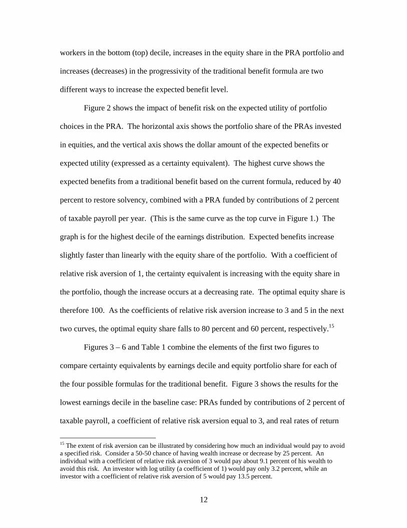
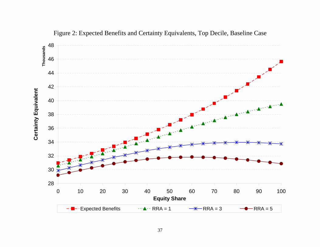
Figure 2 shows the impact of benefit risk on the expected utility of portfolio

choices in the PRA. The horizontal axis shows the portfolio share of the PRAs invested

in equities, and the vertical axis shows the dollar amount of the expected benefits or

expected utility (expressed as a certainty equivalent). The highest curve shows the

expected benefits from a traditional benefit based on the current formula, reduced by 40

percent to restore solvency, combined with a PRA funded by contributions of 2 percent

of taxable payroll per year. (This is the same curve as the top curve in Figure 1.) The

graph is for the highest decile of the earnings distribution. Expected benefits increase

slightly faster than linearly with the equity share of the portfolio. With a coefficient of

relative risk aversion of 1, the certainty equivalent is increasing with the equity share in

the portfolio, though the increase occurs at a decreasing rate. The optimal equity share is

therefore 100. As the coefficients of relative risk aversion increase to 3 and 5 in the next

two curves, the optimal equity share falls to 80 percent and 60 percent, respectively.15

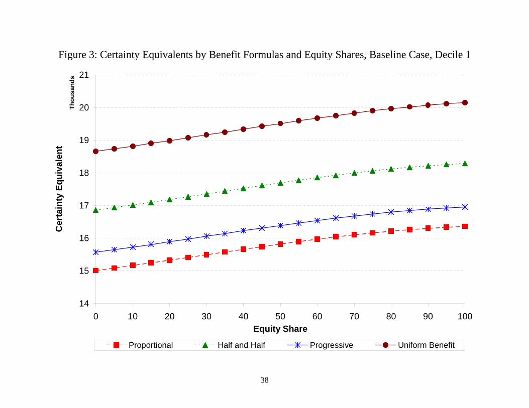
Figures 3 – 6 and Table 1 combine the elements of the first two figures to

compare certainty equivalents by earnings decile and equity portfolio share for each of

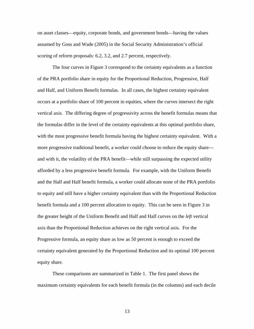
the four possible formulas for the traditional benefit. Figure 3 shows the results for the

lowest earnings decile in the baseline case: PRAs funded by contributions of 2 percent of

taxable payroll, a coefficient of relative risk aversion equal to 3, and real rates of return

15 The extent of risk aversion can be illustrated by considering how much an individual would pay to avoid a specified risk. Consider a 50-50 chance of having wealth increase or decrease by 25 percent. An individual with a coefficient of relative risk aversion of 3 would pay about 9.1 percent of his wealth to avoid this risk. An investor with log utility (a coefficient of 1) would pay only 3.2 percent, while an investor with a coefficient of relative risk aversion of 5 would pay 13.5 percent.

13

on asset classes—equity, corporate bonds, and government bonds—having the values

assumed by Goss and Wade (2005) in the Social Security Administration’s official

scoring of reform proposals: 6.2, 3.2, and 2.7 percent, respectively.

The four curves in Figure 3 correspond to the certainty equivalents as a function

of the PRA portfolio share in equity for the Proportional Reduction, Progressive, Half

and Half, and Uniform Benefit formulas. In all cases, the highest certainty equivalent

occurs at a portfolio share of 100 percent in equities, where the curves intersect the right

vertical axis. The differing degree of progressivity across the benefit formulas means that

the formulas differ in the level of the certainty equivalents at this optimal portfolio share,

with the most progressive benefit formula having the highest certainty equivalent. With a

more progressive traditional benefit, a worker could choose to reduce the equity share—

and with it, the volatility of the PRA benefit—while still surpassing the expected utility

afforded by a less progressive benefit formula. For example, with the Uniform Benefit

and the Half and Half benefit formula, a worker could allocate none of the PRA portfolio

to equity and still have a higher certainty equivalent than with the Proportional Reduction

benefit formula and a 100 percent allocation to equity. This can be seen in Figure 3 in

the greater height of the Uniform Benefit and Half and Half curves on the left vertical

axis than the Proportional Reduction achieves on the right vertical axis. For the

Progressive formula, an equity share as low as 50 percent is enough to exceed the

certainty equivalent generated by the Proportional Reduction and its optimal 100 percent

equity share.

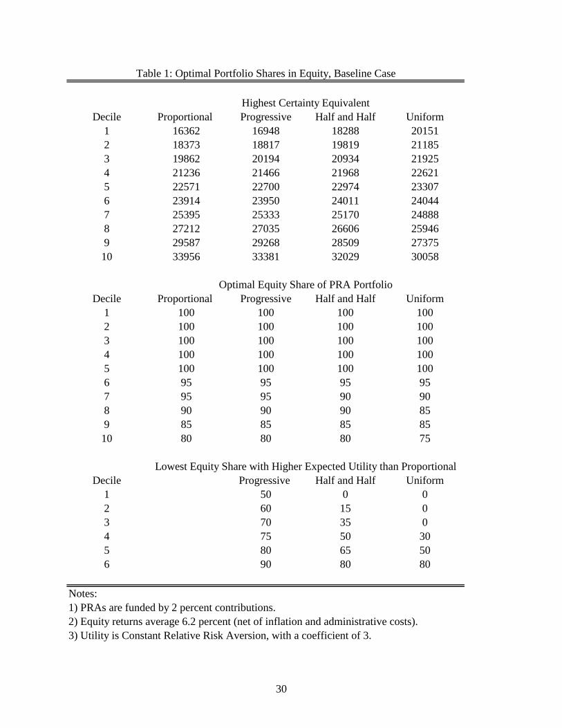
These comparisons are summarized in Table 1. The first panel shows the

maximum certainty equivalents for each benefit formula (in the columns) and each decile

14

of the earnings distribution (in the rows), where the maximum is chosen over equity

shares that are multiples of 5 between 0 and 100. The second panel shows, for each

earnings decile and benefit formula, the equity share that gives that maximum certainty

equivalent. Finally, the bottom panel shows, for all benefit formulas that are not the

Proportional Reduction, the lowest equity share (again, in multiples of 5), that will

surpass the maximum certainty equivalent available under the Proportional Reduction.

This panel will only have rows for earnings deciles in which this is possible. For

example, a Uniform Benefit with an equity share of zero surpasses a Proportional

Reduction with any equity share (including the maximum, at 100 percent) for the lowest

three earnings deciles.

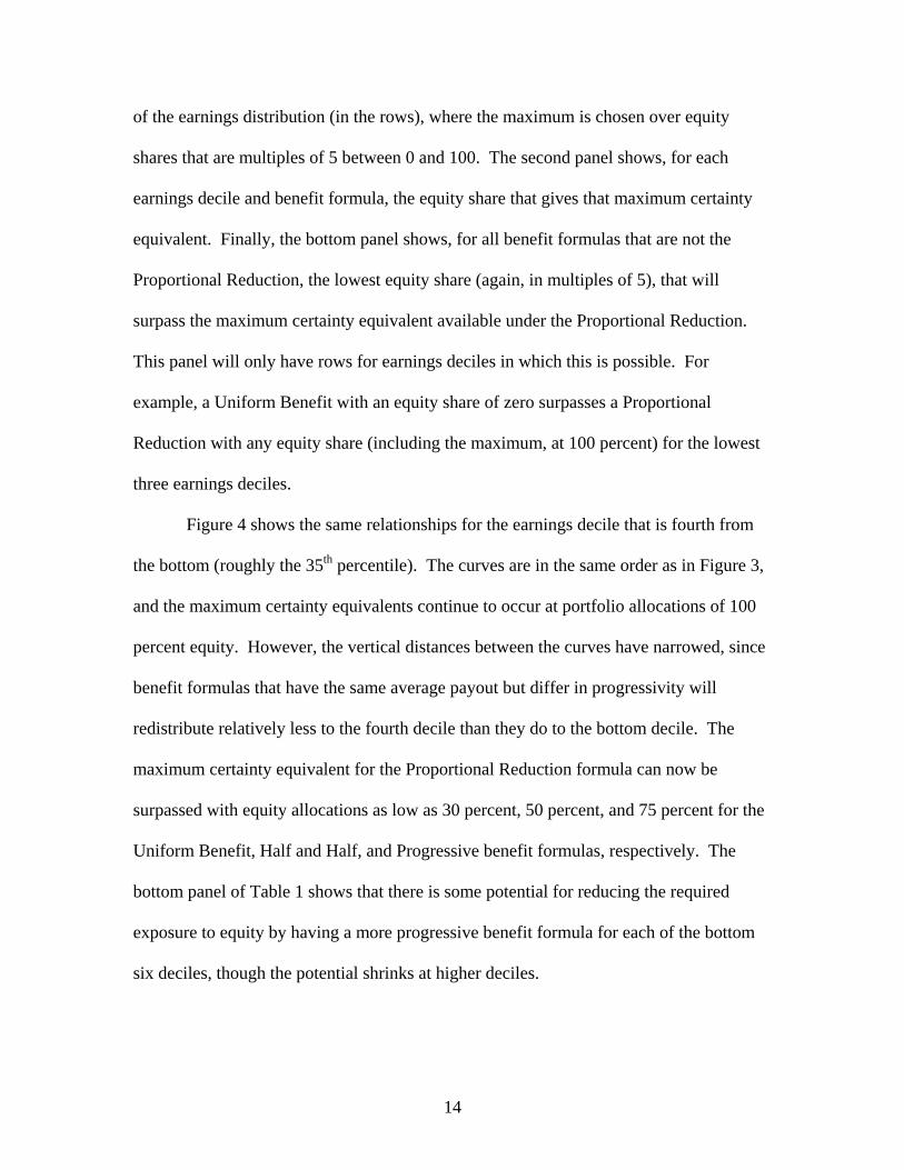
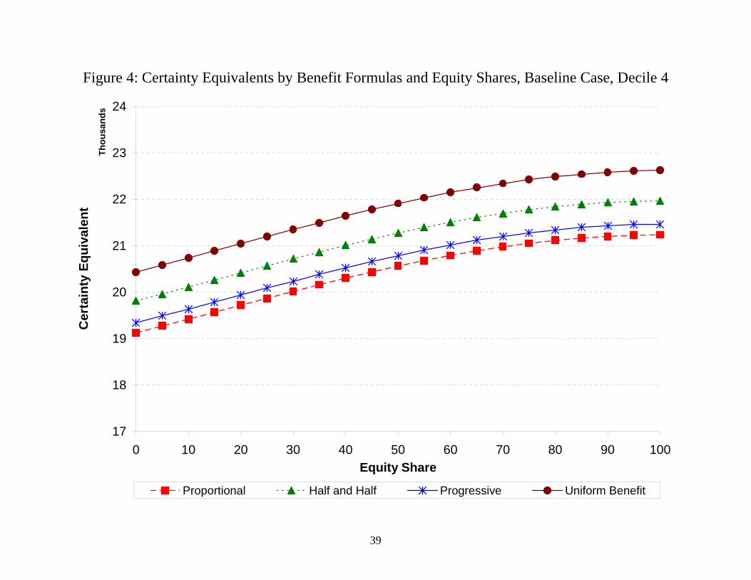
Figure 4 shows the same relationships for the earnings decile that is fourth from

the bottom (roughly the 35th percentile). The curves are in the same order as in Figure 3,

and the maximum certainty equivalents continue to occur at portfolio allocations of 100

percent equity. However, the vertical distances between the curves have narrowed, since

benefit formulas that have the same average payout but differ in progressivity will

redistribute relatively less to the fourth decile than they do to the bottom decile. The

maximum certainty equivalent for the Proportional Reduction formula can now be

surpassed with equity allocations as low as 30 percent, 50 percent, and 75 percent for the

Uniform Benefit, Half and Half, and Progressive benefit formulas, respectively. The

bottom panel of Table 1 shows that there is some potential for reducing the required

exposure to equity by having a more progressive benefit formula for each of the bottom

six deciles, though the potential shrinks at higher deciles.

15

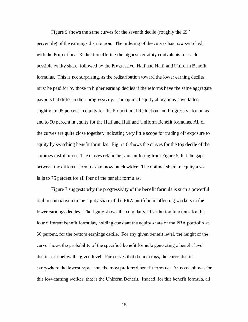
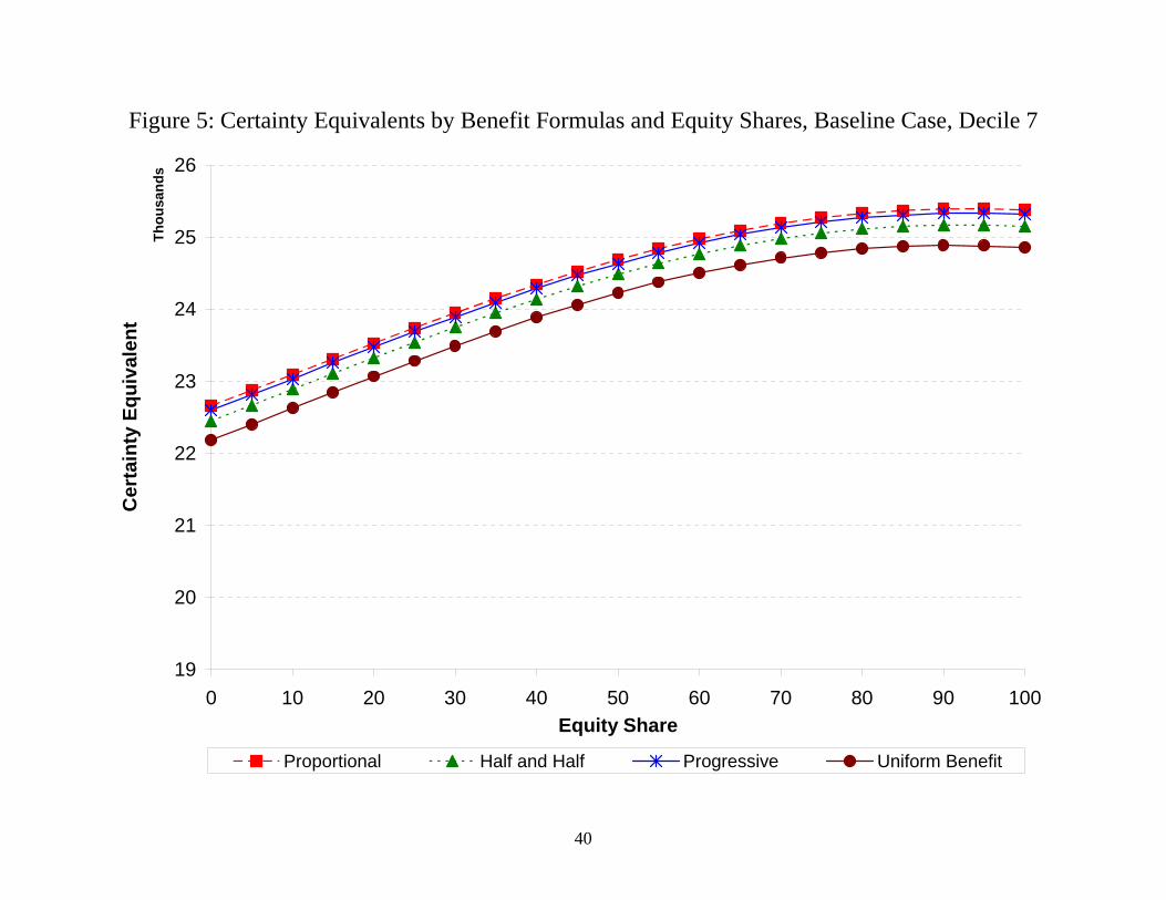
Figure 5 shows the same curves for the seventh decile (roughly the 65th

percentile) of the earnings distribution. The ordering of the curves has now switched,

with the Proportional Reduction offering the highest certainty equivalents for each

possible equity share, followed by the Progressive, Half and Half, and Uniform Benefit

formulas. This is not surprising, as the redistribution toward the lower earning deciles

must be paid for by those in higher earning deciles if the reforms have the same aggregate

payouts but differ in their progressivity. The optimal equity allocations have fallen

slightly, to 95 percent in equity for the Proportional Reduction and Progressive formulas

and to 90 percent in equity for the Half and Half and Uniform Benefit formulas. All of

the curves are quite close together, indicating very little scope for trading off exposure to

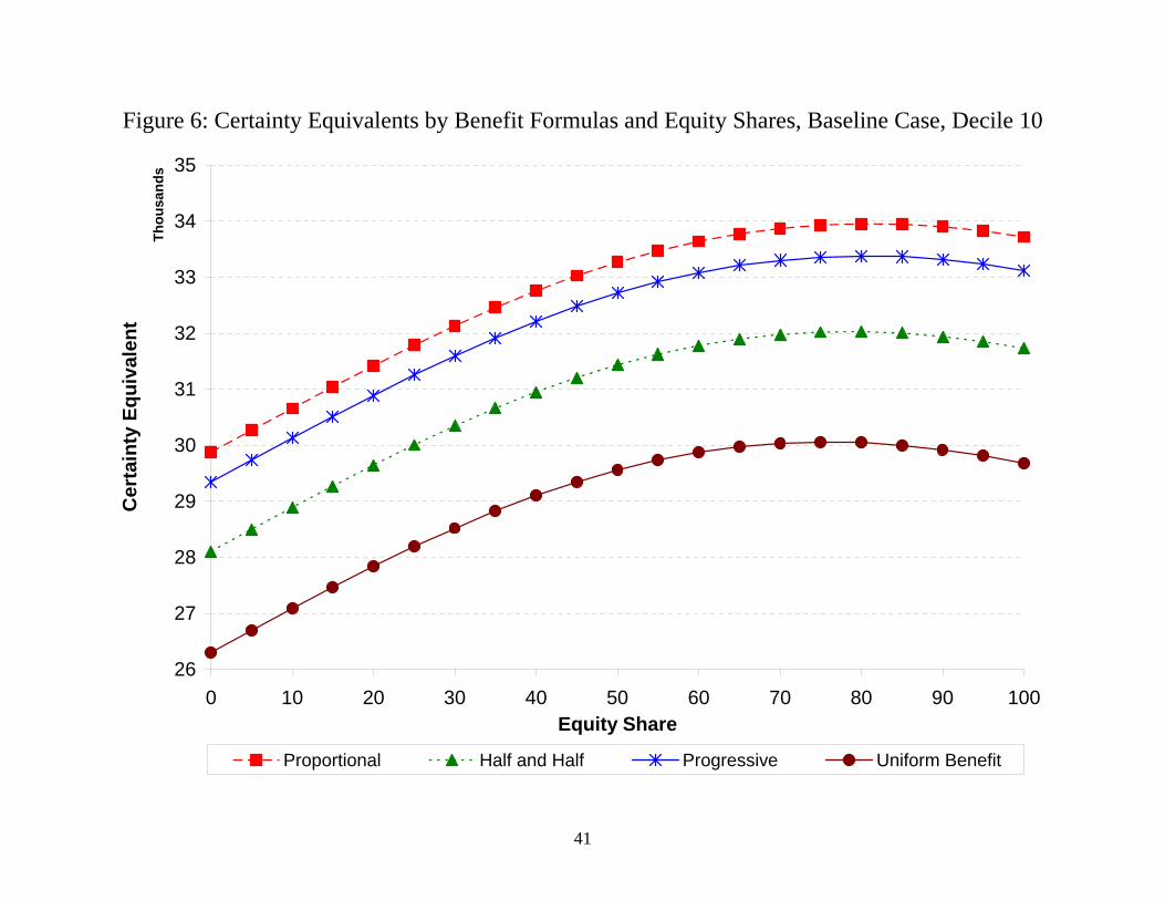
equity by switching benefit formulas. Figure 6 shows the curves for the top decile of the

earnings distribution. The curves retain the same ordering from Figure 5, but the gaps

between the different formulas are now much wider. The optimal share in equity also

falls to 75 percent for all four of the benefit formulas.

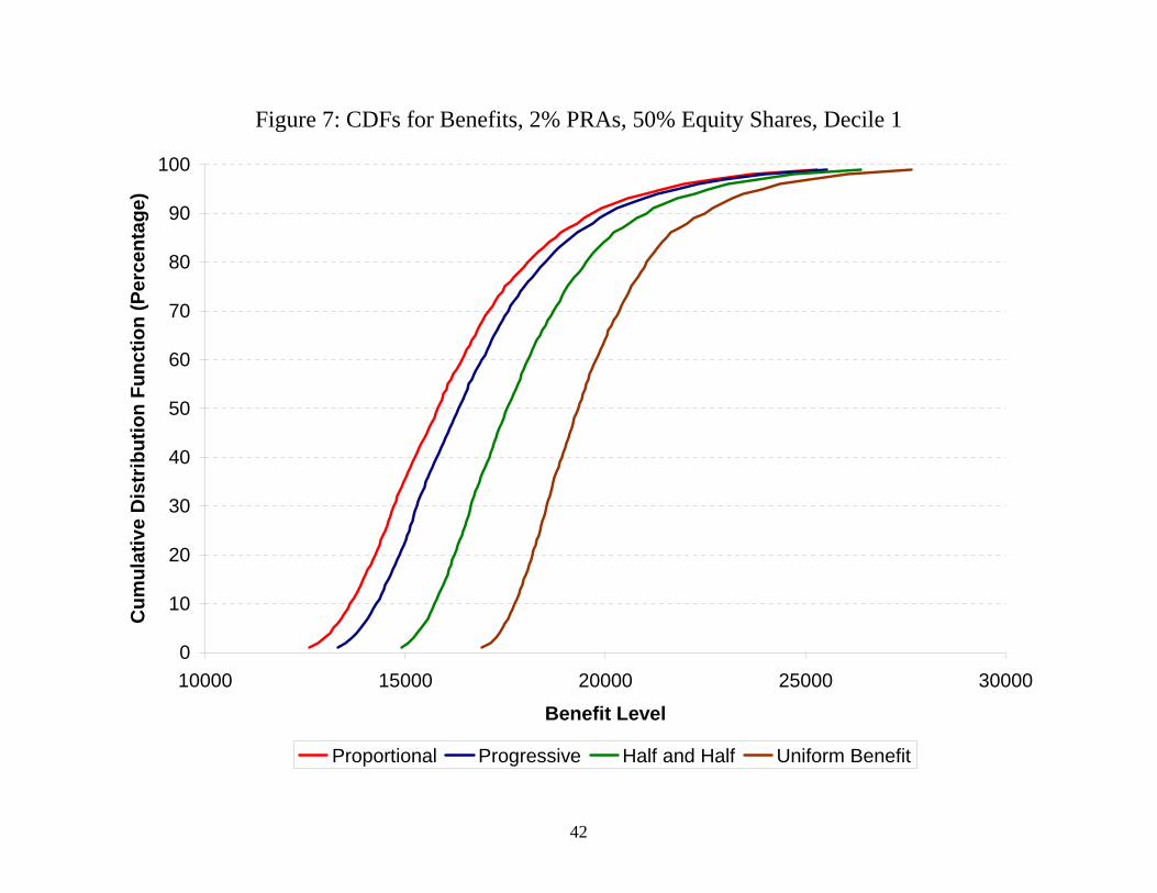
Figure 7 suggests why the progressivity of the benefit formula is such a powerful

tool in comparison to the equity share of the PRA portfolio in affecting workers in the

lower earnings deciles. The figure shows the cumulative distribution functions for the

four different benefit formulas, holding constant the equity share of the PRA portfolio at

50 percent, for the bottom earnings decile. For any given benefit level, the height of the

curve shows the probability of the specified benefit formula generating a benefit level

that is at or below the given level. For curves that do not cross, the curve that is

everywhere the lowest represents the most preferred benefit formula. As noted above, for

this low-earning worker, that is the Uniform Benefit. Indeed, for this benefit formula, all

16

of the variation in benefit levels is due to the variation in asset returns in different

scenarios. Moving right to left on the graph, the other benefit formulas lower average

benefits and add successively more earnings risk into the benefit distributions. The

differences in the lowest benefit amounts across formulas (measured by the horizontal

distance between the curves near the horizontal axis) are quite large. These differences

also persist fairly high into the distribution of benefits, disappearing only at the highest

benefit levels. Given risk averse workers, the level and likelihood of very low outcomes

are of particular concern.

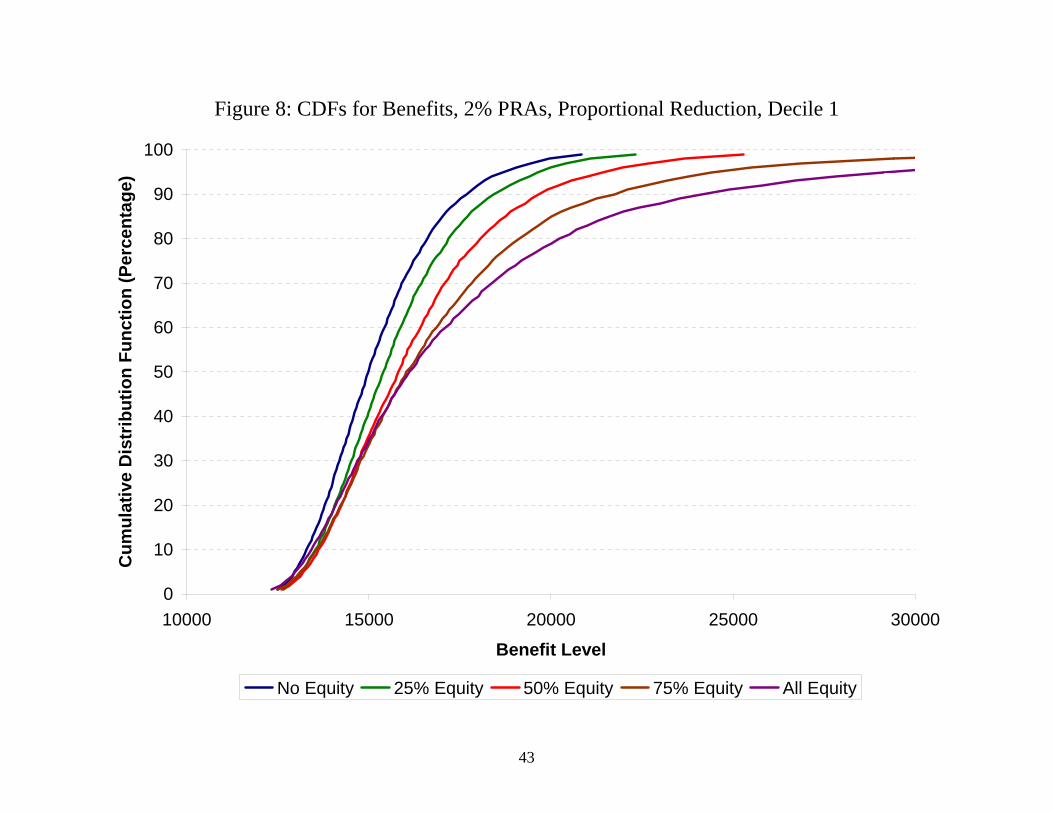
Figure 8 shows the variation in this decile’s benefit distributions holding the

benefit formula fixed (at Proportional Reduction) while varying the equity share in the

portfolio from 0 to 100 percent in increments of 25 percentage points. At the very lowest

benefit levels, the differences across the portfolio allocations are quite small in

comparison to those shown in Figure 7. (The scales on the axes are identical across the

figures.) Low benefit outcomes are primarily due to the factor held constant across the

curves—the traditional benefit formula—rather than the factor varying across the

curves—the equity share in the PRA portfolio. To the extent that there are differences,

both the “All Equity” and “Zero Equity” portfolios have lower minimum benefits than

more balanced portfolios. At the low end of the earnings distribution, reducing the equity

share from 100 percent does not even generate a lower likelihood of very bad outcomes.

These figures establish the main results of the analysis. Given the assumed

average returns on equities and bonds and their historical variation, workers with CRRA

utility and a coefficient of relative risk aversion of 3 typically choose high equity shares

in their PRA portfolios, regardless of the formula used to compute the traditional benefit.

17

However, switching from a proportional reduction in the traditional benefits to any of the

three more progressive benefit formulas increases the traditional benefits going to the

bottom six deciles of the earnings distribution. This increase in traditional benefits gives

the worker room to lower the equity share in the PRA portfolio while still achieving the

same certainty equivalent available with the optimal equity share in the PRA under the

proportionally reduced benefit. In the case of the maximally progressive benefit formula,

in which the traditional benefit is a uniform benefit unrelated to the worker’s earnings,

the equity share could fall to zero for the lowest three deciles. Higher deciles or less

extreme changes to the progressivity of the benefit formula result in somewhat smaller

possible reductions in equity exposure.

VI. Sensitivity Tests

In this section, the robustness of the main results is assessed by varying the degree

of risk aversion, the constancy of the coefficient of relative risk aversion, the equity

premium, and the size of the PRAs measured by the annual contributions as a percentage

of earnings. More risk aversion, declining relative risk aversion, a lower equity premium,

and larger PRAs generally reduce the optimal portfolio allocations in equities and slightly

compress the differences in the allocations across configurations of the traditional benefit

that achieve the same certainty equivalent. This section concludes with a discussion of

life cycle portfolio strategies.

18

Risk Aversion

The baseline choice of the coefficient of risk aversion is consistent with

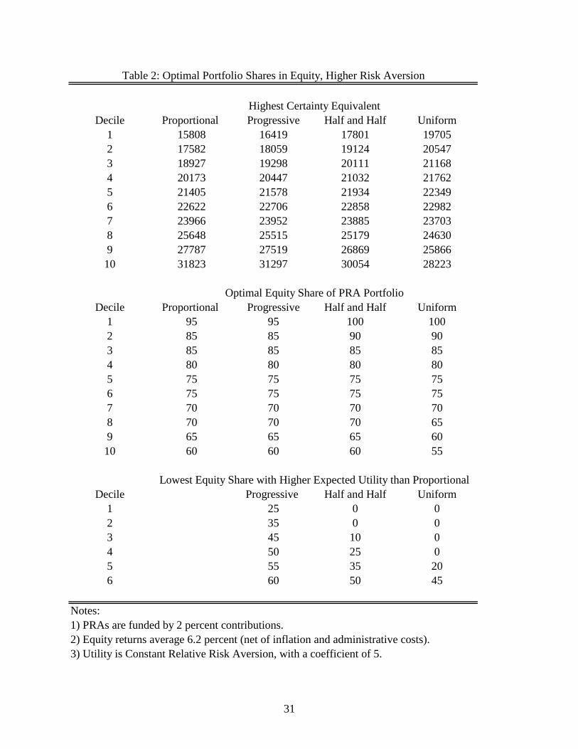
assumptions found in the literature on insurance and risk. Table 2 repeats the analysis of

Table 1 for a higher coefficient of relative risk aversion equal to 5. The first consequence

of higher relative risk aversion is that all of the certainty equivalents in the top panel of

Table 2 are lower than their counterparts in Table 1. Consistent with Figure 2, a worker

with higher risk aversion would pay a greater risk premium to avoid a given risk. The

next panel of Table 2 shows that the workers seek to avoid this risk by reducing their

equity shares in the PRA portfolio.16 For example, with the Proportional Reduction,

optimal equity shares are 95 percent in the lowest earnings decile, falling to 60 percent by

the highest earnings decile.

As shown in the bottom panel of the table, changes in the progressivity of the

traditional benefit allow for reductions in equity exposure in the PRA portfolio that are

comparable to those for the less risk averse workers in Table 1. For example, it is still the

case that the bottom six earnings deciles have room to lower their equity exposure with

more progressive traditional benefit formulas. In addition, the allowable percentage point

reductions in the equity shares are similar. For example, with a Uniform Benefit, the

bottom four deciles can now eliminate their equity exposure entirely. With the

Progressive benefit formula, the equity share for the bottom earnings decile can fall from

95 to 25 percent without a loss in expected utility. Thus, the main results are robust to a

higher coefficient of relative risk aversion.

16 In other words, the certainty equivalents would be even lower if the workers were constrained to hold the equity shares at the levels in the middle panel of Table 1.

19

Declining Relative Risk Aversion

The results in the middle panels of Tables 1 and 2 show that the optimal

allocation to equity declines at higher earnings deciles. This pattern arises due to the

maintained assumption in the simulations that workers have no other sources of

retirement income apart from the traditional benefit and the PRA. Because even the

current Social Security formula is progressive, workers in lower earnings deciles have a

greater proportion of their retirement benefits insulated from investment risk. With a

homothetic expected utility function, this enables lower earning workers to take on more

equity risk in their PRA portfolios.17

This pattern is counterfactual—in reality, investment allocations to equity rise

dramatically with earnings.18 One way to make the simulations more consistent with

observed investment behavior is to modify the expected utility function to exhibit

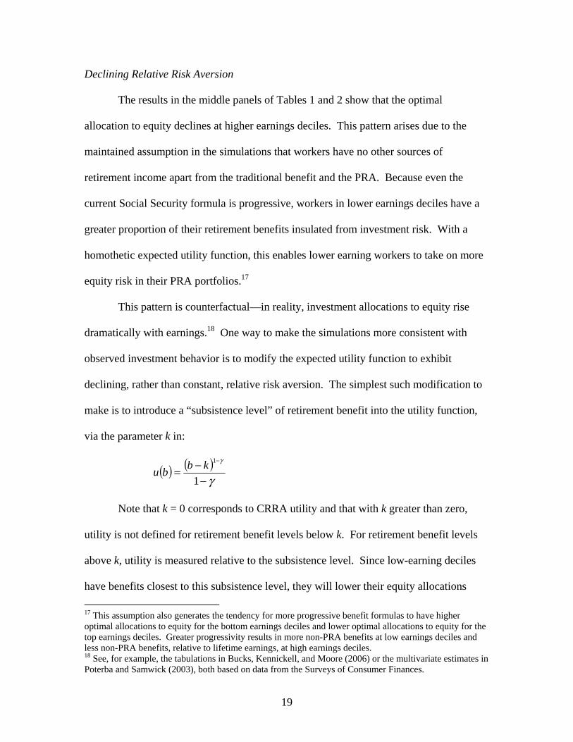
declining, rather than constant, relative risk aversion. The simplest such modification to

make is to introduce a “subsistence level” of retirement benefit into the utility function,

via the parameter k in:

( ) ( )γ

γ

−−=

−

1

1kbbu

Note that k = 0 corresponds to CRRA utility and that with k greater than zero,

utility is not defined for retirement benefit levels below k. For retirement benefit levels

above k, utility is measured relative to the subsistence level. Since low-earning deciles

have benefits closest to this subsistence level, they will lower their equity allocations 17 This assumption also generates the tendency for more progressive benefit formulas to have higher optimal allocations to equity for the bottom earnings deciles and lower optimal allocations to equity for the top earnings deciles. Greater progressivity results in more non-PRA benefits at low earnings deciles and less non-PRA benefits, relative to lifetime earnings, at high earnings deciles. 18 See, for example, the tabulations in Bucks, Kennickell, and Moore (2006) or the multivariate estimates in Poterba and Samwick (2003), both based on data from the Surveys of Consumer Finances.

20

relative to the CRRA case. The certainty equivalent for this DRRA expected utility

function is given by:

( ) ( )( )[ ] ( ) ( )( )[ ] ( )γγγγ−−− −+=−+=

111111 kbEkbuEkbCE

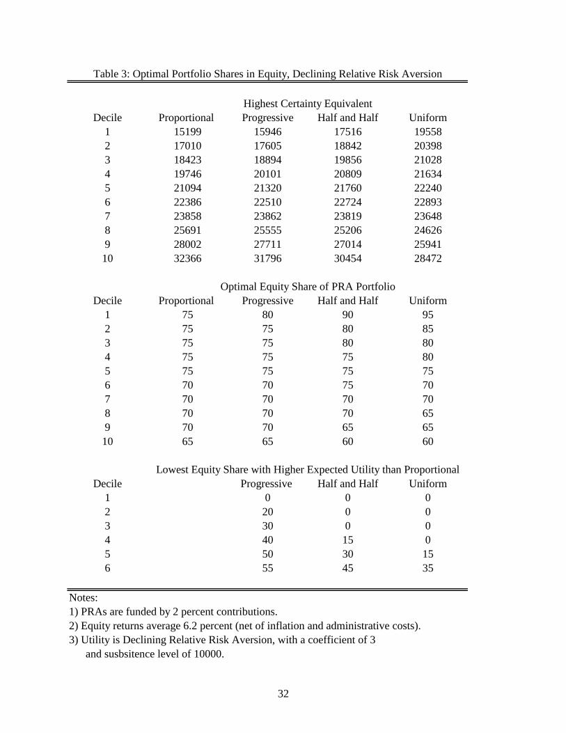
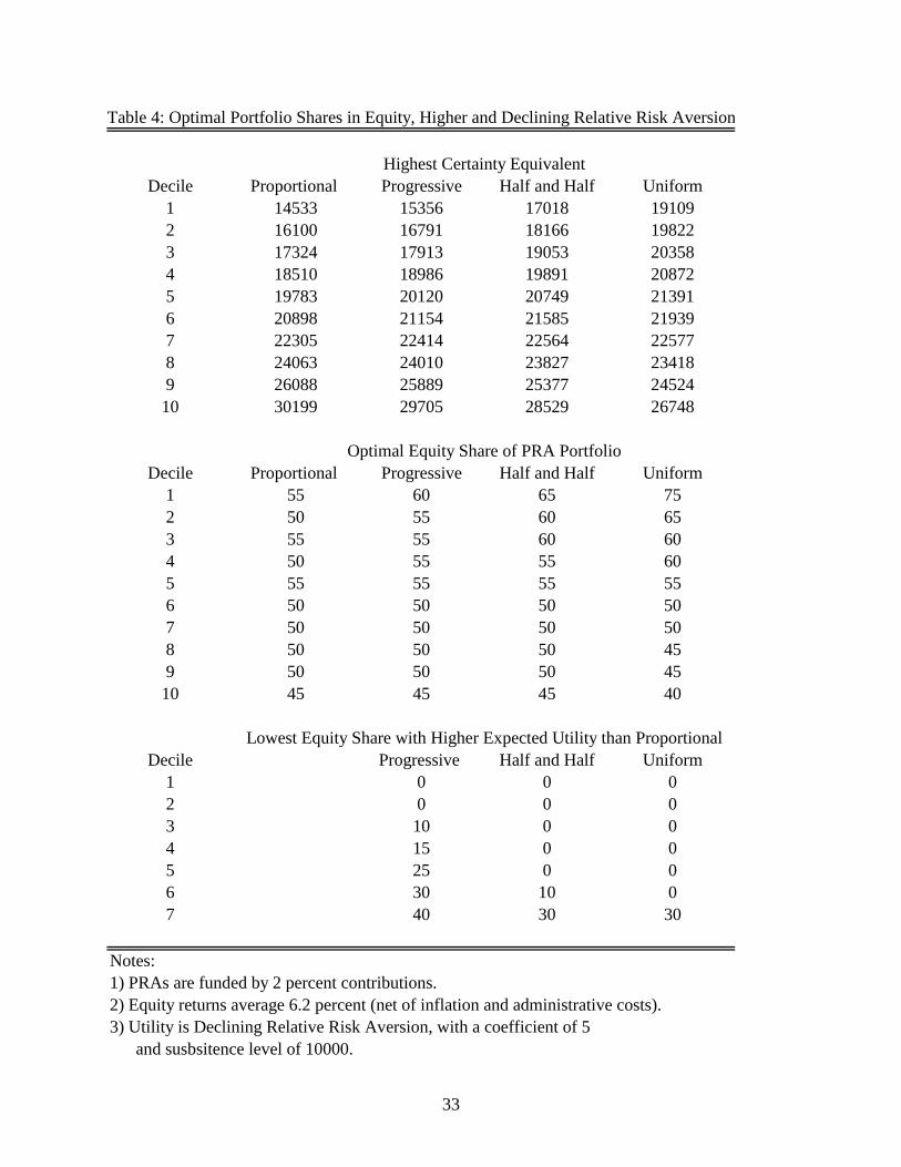
Tables 3 and 4 repeat the analyses in Tables 1 and 2 using this DRRA expected

utility function. The subsistence level is assumed to be $10,000, which is close to the

minimum benefit for the lowest earning decile shown in Figure 7. The top panels of the

tables show that the certainty equivalents are lower when expected utility exhibits

declining rather than constant relative risk aversion.19 The middle panels of the tables

show that optimal equity allocations are also lower with declining relative risk aversion.

However, comparisons of the changes in the optimal equity allocations by

earnings decile and across traditional benefit formulas relative to the CRRA case are not

straightforward. For example, with γ = 3, equity shares with a Proportional Reduction in

the traditional benefit fall from 75 to 65 percent over the earnings deciles, compared to a

decline from 100 to 80 percent in the CRRA case, indicating less sensitivity to earnings

decile. However, with a Uniform Benefit, they fall from 95 to 60 percent over the

earnings deciles, compared to a decline from 100 to 75 percent in the CRRA case,

indicating more sensitivity to earnings decile. Similar results hold for the higher risk

aversion in Table 4 and in the differences across columns in the respective cases.

Nonetheless, the bottom panels of the tables show that changing from a

Proportional Reduction to a more progressive benefit formula can lessen equity exposure

by as much or more than in the CRRA case. For example, with γ = 3, the bottom six

19 The degree of relative risk aversion for any expected utility function is given by –b*u’’( )/u’( ). For the DRRA utility function, this expression is γ*b/(b – k), which is equal to the constant γ for k = 0. When k > 0, this expression declines toward γ as b increases.

21

deciles can again have their equity exposure reduced. With a Uniform Benefit, the

bottom four deciles can reduce equity exposure to zero without falling behind the

Proportional Reduction. The sixth decile can lower its equity share from 70 to 35

percent, compared to a reduction from 95 to 80 percent in the CRRA case shown in Table

1. With the Progressive formula, the bottom decile can reduce its equity exposure down

to zero and the sixth decile can reduce its equity share from 75 to 55 percent (compared

to a reduction from 95 to 90 percent in the CRRA case). The results in Table 4 at higher

risk aversion levels are even more pronounced. Thus, the main results shown in the

previous section are robust to and strengthened by a switch to an expected utility function

that exhibits declining rather than constant relative risk aversion.

Lower Equity Premium

The sustainability of the premium that has existed to investments in equities

historically has been the subject of considerable debate. Particularly in the case of

financial market returns, past performance may be an unreliable guide to future

outcomes. For example, if over the past 30 years, systematic risk in the stock market fell,

then the appropriate rate of return to assume going forward would be lower. However,

during this period of time that risk fell, the reduction in risk would have generated

abnormally high returns to equity. These high holding period returns would have arisen

precisely because future ex ante returns had fallen and would thus be a poor guide to

forecasting those future returns.20

20 For a discussion of the issues associated with choosing a real return on stocks for the long term, see the papers by John Campbell, Peter Diamond, and John Shoven in Social Security Advisory Board (2001).

22

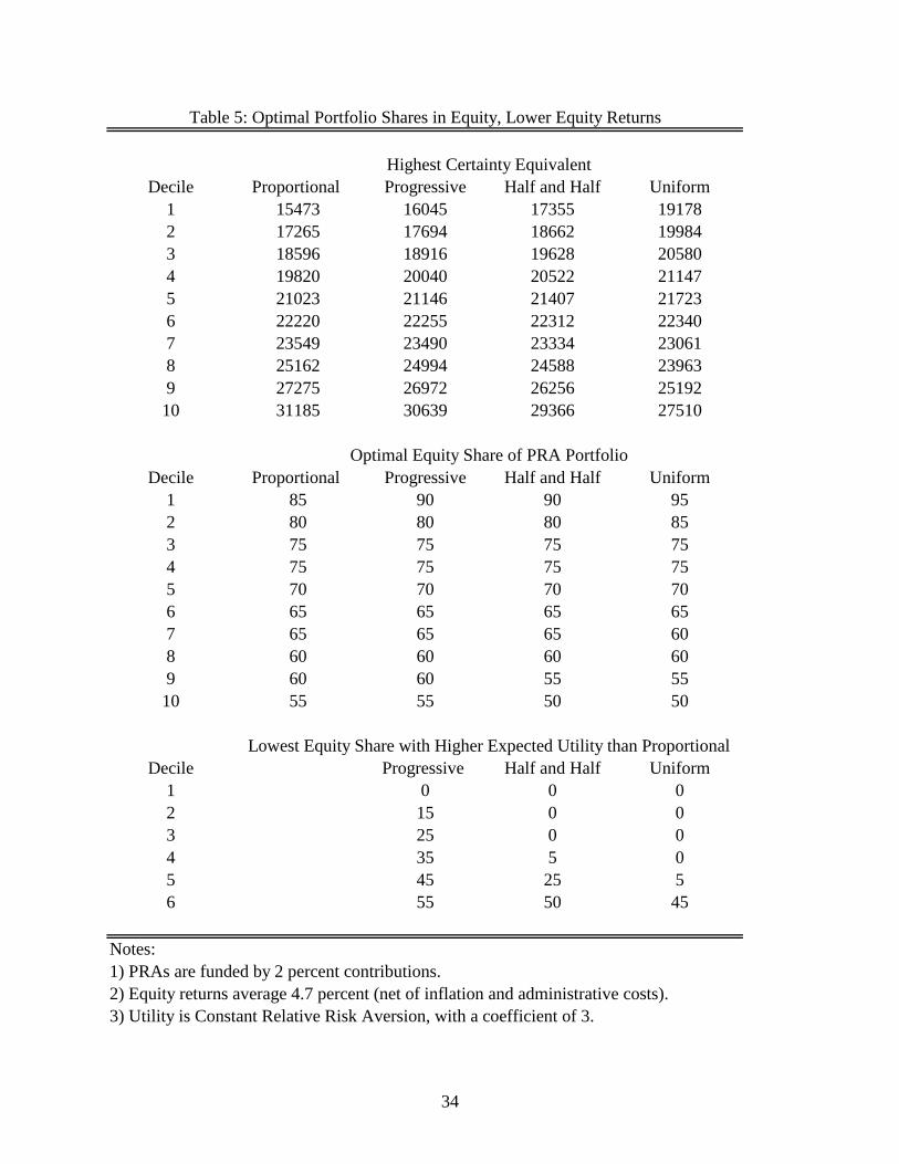
In light of such considerations, Table 5 reports the results of simulations in which

the expected return on equities is lowered from 6.2 percent to 4.7 percent. PRA

contributions remain 2 percent of earnings per year, and the comparisons are shown for a

CRRA utility function with a relative risk aversion coefficient of 3. As expected, the 150

basis point reduction in the equity premium lowers the certainty equivalents for all

earnings deciles and benefit formulas, shown in the top panel. The lower equity premium

also shifts the optimal portfolio allocations to equity lower. For the Proportional

Reduction, equity shares range from 85 to 55 percent, compared to 100 to 80 percent in

Table 1. For the Uniform Benefit, equity shares range from 95 to 50 percent, compared

to 100 to 75 percent in Table 1.

With a lower equity premium, there is greater scope for changes in the

progressivity of the benefit formula to substitute for higher equity allocations. The

bottom panel of Table 5 shows that with a Uniform Benefit, the bottom four deciles can

reduce their equity shares to zero to keep pace with the optimal allocations of 75 to 85

percent in the Proportional Reduction case. The sixth decile can reduce its equity share

to 45 percent from 65 percent. In Table 1, with the higher equity premium, this decile

could reduce its equity share only to 80 percent from 95 percent. Possible reductions in

equity exposure for other benefit formulas are smaller than with the Uniform Benefit

formula but similarly larger than their counterparts with the higher equity premium in

Table 1. Thus, the main results in the previous section are robust and even strengthened

in the presence of a lower equity premium.

23

Larger Personal Retirement Accounts

Compared to the investment-based reform plans that have been proposed (see

footnote 2), a PRA funded by only a 2 percent contribution is fairly small. The ability of

progressivity in the traditional benefit to offset financial risk in the PRAs depends on the

relative size of the two benefits. To investigate this dependence and extend the analysis

to cover more of the range of proposed reforms, Table 6 presents the results of

simulations in which the annual PRA contribution is increased from 2 to 3 percent of

earnings. The certainty equivalents in the top panel are all naturally higher than their

counterparts in Table 1, since the additional 1-percent contributions are not accounted for

by reduced consumption elsewhere in this framework. The middle panel of the table

shows that optimal equity allocations are slightly lower with the larger PRAs. As the

PRAs get larger relative to the traditional benefit, workers seek to mitigate their risk

exposure through lower allocations to equity.

The bottom panel shows that the ability to offset equity exposure through more

progressive traditional benefit formulas can be slightly lower or higher, depending on the

earnings decile and benefit formula. With a Uniform Benefit, the bottom two deciles can

reduce their equity shares to zero to keep pace with the optimal allocations of 95 to 100

percent in the Proportional Reduction case. In Table 1, with the smaller PRAs, the

bottom three deciles could eliminate all equity exposure. The sixth decile can reduce its

equity share to 65 percent from 85 percent, compared to a reduction to 80 percent from

95 percent in Table 1. For the Progressive benefit formula, reductions in equity exposure

relative to the Proportional Reduction formula are comparable to those in Table 1.

24

Life Cycle Portfolios

As noted above, prior studies have analyzed the use of life cycle investment

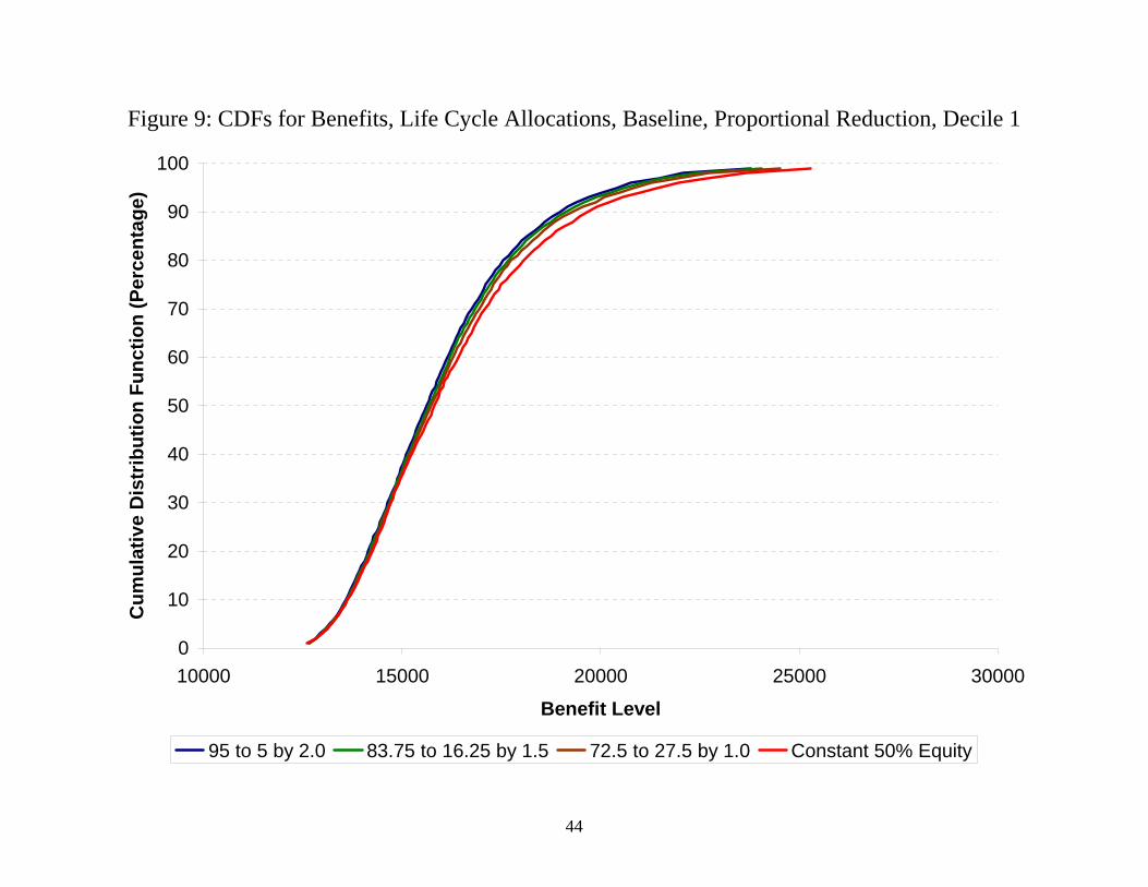
strategies to mitigate financial risk in PRAs. Figure 9 compares a portfolio with an age-

invariant allocation of 50 percent to equity with three life cycle strategies that shift from

equity to bonds as retirement approaches. The first starts at a 95 percent equity share and

decreases 2 percentage points per year, reaching 5 percent on the eve of retirement. The

second starts at an 83.75 percent equity share and decreases 1.5 percentage points per

year, reaching 16.25 percent on the eve of retirement. The third starts at a 72.5 percent

equity share and decreases by 1 percentage point per year, reaching 27.5 percent on the

eve of retirement. All three strategies are centered on a 50 percent equity share, based on

the simple average of the allocation rules by age. The figure pertains to the lowest

earnings decile and shows the cumulative distribution functions for each of the four

investment options.

There are two important features of the graph. First, the curves all lie virtually on

top of each other. There cannot be much of an improvement in expected utility by

switching to a life cycle strategy if such a strategy results in a distribution of benefits that

is so similar to the age-invariant portfolio allocation. Second, the life cycle strategies lie

above the age-invariant portfolio for all but the very lowest percentiles of the

distributions, the more so the greater the decline in the equity allocation with age. The

reason is that the life cycle strategies do not have the same expected benefits as the age-

invariant portfolio, because the life cycle strategies focus the high-equity allocations on

the early years, when many years of contributions are yet to be made.

25

Thus, life cycle strategies may be desirable, but this is so in the current context

primarily because they serve to reduce the overall level of equity exposure. This may be

a desirable goal—for example, if the equity premium is low enough or volatility of

returns is high enough—but it can be achieved more straightforwardly with a simple

reduction in the age-invariant portfolio share in equities given the parameters used in the

simulations above.

VII. Conclusions

Policy makers seeking to design investment-based Social Security reform

proposals have wrestled with the issue of how much financial risk is appropriate for

individuals to bear. Suggested methods of alleviating risk have focused on strategies that

amount to requiring more bonds relative to equity in the Personal Retirement Accounts,

whether through the purchase of guarantees or life cycle investment strategies. It is

worth emphasizing that most of the simulations in this paper suggest fairly high optimal

allocations to equities, particularly by those in the lowest deciles of the earnings

distribution. Direct restrictions on equity holding in PRAs are likely to prove unpopular,

particularly among those whose opportunities are most broadened by the chance to invest

their mandatory contributions in equities. This paper suggests another possibility for

alleviating the consequences of financial risk; namely, increasing the progressivity of the

traditional benefit. Doing so insulates workers in the lower part of the benefit

distribution against possibly adverse shocks to financial returns without constraining

them to not invest in equities.

26

The main simulations in the paper compare proportional reductions in traditional

benefits with more progressive reductions. The key finding is that under baseline

parameters, the most progressive traditional benefit—a flat benefit independent of

earnings—allows the allocation to equities to be reduced to zero for the lowest three

earnings deciles relative to the optimal allocation when the traditional benefits are

reduced proportionately based on the current formula. The next three deciles are able to

achieve some reduction in equity exposure as well. Under less extreme changes to the

traditional benefit, such as that proposed by Liebman, MacGuineas, and Samwick (2005),

the allocation to equities can be decreased by half for the lowest earnings decile and by

smaller fractions for an additional five deciles. Sensitivity tests show that optimal

allocations to equities typically decrease with higher risk aversion, declining risk

aversion, a lower equity premium, or larger accounts, but the general pattern of results

persists and in some cases allows for greater equity reduction through higher

progressivity in the traditional benefit formula.

The results in this paper suggest two avenues for further research. First, the

present analysis used a very stylized model of the initial earnings distribution and its

evolution over time to simulate the distribution of future benefits. Actual data and more

sophisticated time-series estimates could be incorporated. Second, the present analysis

focused on time-invariant portfolio allocations in the PRAs, which were further assumed

to be the worker’s only source of investment wealth. While the latter might be a

reasonable approximation for the lowest earning households, higher earning households

are likely to have existing holdings of equities that make the portfolio allocation decision

in the PRA less consequential. Extending the current framework to allow for optimal,

27

age-dependent portfolio allocations and for saving in accounts other than the PRAs would

provide better estimates of the extent to which greater progressivity can protect low

earners from investment risk and of the size of the welfare costs paid by higher earners

for providing this protection.

28

References

The Board of Trustees, Federal Old-Age and Survivors Insurance and Federal Disability Insurance Trust Funds (2006). Annual Report. Washington: U.S. Government Printing Office. [Cited as “Social Security Trustees Report 2006.”] http://www.ssa.gov/OACT/TR/TR06/tr06.pdf Bucks, Brian K., Arthur B. Kennickell, and Kevin B. Moore (2006). “Recent Changes in U.S. Family Finances: Evidence from the 2001 and 2004 Survey of Consumer Finances,” Federal Reserve Bulletin, Vol. 92 (February 2006): A1-A38. http://www.federalreserve.gov/pubs/oss/oss2/2004/bull0206.pdf Feldstein, Martin S. and Elena Ranguelova (2001a). “Accumulated Pension Collars: A Market Approach to Reducing The Risk of Investment-Based Social Security Reform,” in James M. Poterba (ed.) Tax Policy and the Economy 2000. Cambridge: MIT Press. Feldstein, Martin S. and Elena Ranguelova (2001b). “Individual Risk in an Investment-Based Social Security System,” American Economic Review, Vol. 91, No. 4 (September): 1116-25. Goss, Stephen C. and Alice H. Wade (2005). “Estimated Financial Effects of ‘A Nonpartisan Approach to Reforming Social Security – A Proposal Developed by Jeffrey Liebman, Maya MacGuineas and Andrew Samwick.’” Manuscript, Social Security Administration, November 17. http://www.ssa.gov/OACT/solvency/Liebman_20051117.pdf Hubbard, R. Glenn, Jonathan S. Skinner, and Stephen P. Zeldes (1994). “The Importance of Precautionary Motives in Explaining Individual and Aggregate Saving,” Carnegie Rochester Conference Series on Public Policy, Vol. 40, 59 – 125. Ibbotson Associates (2006). Stocks, Bonds, Bills, and Inflation Yearbook 2006. Chicago: Ibbotson Associates. Kunkel, Jeffrey L. (1996). “Frequency Distribution of Wage Earners by Wage Level,” Actuarial Note, No. 135. Washington: Social Security Administration, Office of the Actuary, July. http://www.ssa.gov/OACT/NOTES/pdf_notes/note135.pdf Liebman, Jeffrey, Maya MacGuineas, and Andrew Samwick (2005). “Nonpartisan Social Security Reform Plan,” Manuscript, Harvard University, December. http://www.ksg.harvard.edu/jeffreyliebman/lms_nonpartisan_plan_description.pdf Poterba, James, Joshua Rauh, Steven Venti, and David Wise (2006). “Lifecycle Asset Allocation Strategies and the Distribution of 401(k) Retirement Wealth,” National Bureau of Economic Research, Working Paper No. 11974, January. http://www.nber.org/papers/w11974

29

Poterba, James and Andrew A. Samwick (2003). “Taxation and Household Portfolio Composition: U.S. Evidence from the 1980s and 1990s,” Journal of Public Economics, Vol. 87 (January): 5-38. Samwick, Andrew A. (1999). “Social Security Reform in the United States.” National Tax Journal, 52 (December), 819 – 842. Samwick, Andrew A. (2004). “Social Security Reform: The United States in 2002.” in Einar Overbye and Peter A. Kemp (eds.) Pensions: Challenges and Reform. Aldershot: Ashgate Publishing Limited, 53-69. Social Security Administration, Office of Policy (2006). Annual Statistical Supplement to the Social Security Bulletin, 2005. Washington: Social Security Administration, February. [Cited as SSA (2006)] http://www.socialsecurity.gov/policy/docs/statcomps/supplement/2005/ Social Security Advisory Board (2001). “Estimating the Real Rate of Return on Stocks Over the Long Term,” August. http://www.ssab.gov/Publications/Financing/estimated%20rate%20of%20return.pdf Topel, Robert H. and Michael P. Ward (1992). “Job Mobility and the Careers of Young Men,” The Quarterly Journal of Economics, Vol. 107, No. 2. (May): 439-479. World Bank (1994). Averting the Old Age Crisis: Policies to Protect the Old and Promote Growth. New York: Oxford University Press.

30

Decile Proportional Progressive Half and Half Uniform1 16362 16948 18288 201512 18373 18817 19819 211853 19862 20194 20934 219254 21236 21466 21968 226215 22571 22700 22974 233076 23914 23950 24011 240447 25395 25333 25170 248888 27212 27035 26606 259469 29587 29268 28509 27375

10 33956 33381 32029 30058


10 80 80 80 75

Decile Progressive Half and Half Uniform1 50 0 02 60 15 03 70 35 04 75 50 305 80 65 506 90 80 80

1) PRAs are funded by 2 percent contributions.2) Equity returns average 6.2 percent (net of inflation and administrative costs).3) Utility is Constant Relative Risk Aversion, with a coefficient of 3.

Lowest Equity Share with Higher Expected Utility than Proportional

Table 1: Optimal Portfolio Shares in Equity, Baseline Case

Notes:

Highest Certainty Equivalent

Optimal Equity Share of PRA Portfolio

31


10 31823 31297 30054 28223


10 60 60 60 55



Table 2: Optimal Portfolio Shares in Equity, Higher Risk Aversion




Notes:

32


10 32366 31796 30454 28472


10 65 65 60 60


1) PRAs are funded by 2 percent contributions.2) Equity returns average 6.2 percent (net of inflation and administrative costs).3) Utility is Declining Relative Risk Aversion, with a coefficient of 3 and susbsitence level of 10000.

Table 3: Optimal Portfolio Shares in Equity, Declining Relative Risk Aversion




Notes:

33

Decile Proportional Progressive Half and Half Uniform1 14533 15356 17018 191092 16100 16791 18166 198223 17324 17913 19053 203584 18510 18986 19891 208725 19783 20120 20749 213916 20898 21154 21585 219397 22305 22414 22564 225778 24063 24010 23827 234189 26088 25889 25377 2452410 30199 29705 28529 26748

Decile Proportional Progressive Half and Half Uniform1 55 60 65 752 50 55 60 653 55 55 60 604 50 55 55 605 55 55 55 556 50 50 50 507 50 50 50 508 50 50 50 459 50 50 50 4510 45 45 45 40

Decile Progressive Half and Half Uniform1 0 0 02 0 0 03 10 0 04 15 0 05 25 0 06 30 10 07 40 30 30

1) PRAs are funded by 2 percent contributions.2) Equity returns average 6.2 percent (net of inflation and administrative costs).3) Utility is Declining Relative Risk Aversion, with a coefficient of 5 and susbsitence level of 10000.

Notes:

Table 4: Optimal Portfolio Shares in Equity, Higher and Declining Relative Risk Aversion




34


10 31185 30639 29366 27510


10 55 55 50 50



Table 5: Optimal Portfolio Shares in Equity, Lower Equity Returns




Notes:

35


10 39522 38941 37579 35590


10 70 70 70 65



Table 6: Optimal Portfolio Shares in Equity, Larger PRAs




Notes:

36

Figure 1: Expected Benefits by Benefit Formula and Equity Share

0

5

10

15

20

25

30

35

40

45

50

0 10 20 30 40 50 60 70 80 90 100

Thou

sand

s

Equity Share

Expe

cted

Ben

efits

37

Figure 2: Expected Benefits and Certainty Equivalents, Top Decile, Baseline Case

28

30

32

34

36

38

40

42

44

46

48

0 10 20 30 40 50 60 70 80 90 100

Thou

sand

s

Equity Share

Cer

tain

ty E

quiv

alen

t

Expected Benefits RRA = 1 RRA = 3 RRA = 5

38

Figure 3: Certainty Equivalents by Benefit Formulas and Equity Shares, Baseline Case, Decile 1

14

15

16

17

18

19

20

21

0 10 20 30 40 50 60 70 80 90 100

Thou

sand

s

Equity Share

Cer

tain

ty E

quiv

alen

t

Proportional Half and Half Progressive Uniform Benefit

39


17

18

19

20

21

22

23

24

0 10 20 30 40 50 60 70 80 90 100

Thou

sand

s

Equity Share

Cer

tain

ty E

quiv

alen

t


40


19

20

21

22

23

24

25

26

0 10 20 30 40 50 60 70 80 90 100

Thou

sand

s

Equity Share

Cer

tain

ty E

quiv

alen

t


41


26

27

28

29

30

31

32

33

34

35

0 10 20 30 40 50 60 70 80 90 100

Thou

sand

s

Equity Share

Cer

tain

ty E

quiv

alen

t


42

Figure 7: CDFs for Benefits, 2% PRAs, 50% Equity Shares, Decile 1

0

10

20

30

40

50

60

70

80

90

100

10000 15000 20000 25000 30000

Benefit Level

Cum

ulat

ive

Dis

trib

utio

n Fu

nctio

n (P

erce

ntag

e)

Proportional Progressive Half and Half Uniform Benefit

43

Figure 8: CDFs for Benefits, 2% PRAs, Proportional Reduction, Decile 1

0

10

20

30

40

50

60

70

80

90

100

10000 15000 20000 25000 30000

Benefit Level

Cum

ulat

ive

Dis

trib

utio

n Fu

nctio

n (P

erce

ntag

e)

No Equity 25% Equity 50% Equity 75% Equity All Equity

44

Figure 9: CDFs for Benefits, Life Cycle Allocations, Baseline, Proportional Reduction, Decile 1

0

10

20

30

40

50

60

70

80

90

100

10000 15000 20000 25000 30000

Benefit Level

Cum

ulat

ive

Dis

trib

utio

n Fu

nctio

n (P

erce

ntag

e)

95 to 5 by 2.0 83.75 to 16.25 by 1.5 72.5 to 27.5 by 1.0 Constant 50% Equity

45

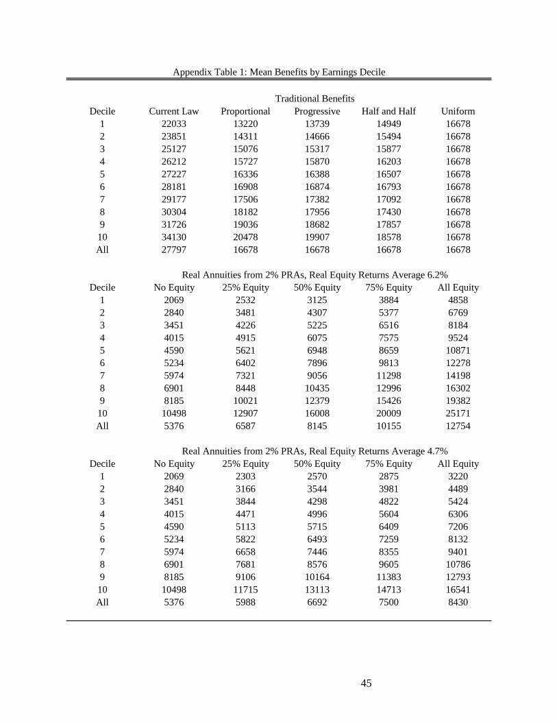
Decile Current Law Proportional Progressive Half and Half Uniform1 22033 13220 13739 14949 166782 23851 14311 14666 15494 166783 25127 15076 15317 15877 166784 26212 15727 15870 16203 166785 27227 16336 16388 16507 166786 28181 16908 16874 16793 166787 29177 17506 17382 17092 166788 30304 18182 17956 17430 166789 31726 19036 18682 17857 1667810 34130 20478 19907 18578 16678All 27797 16678 16678 16678 16678

Decile No Equity 25% Equity 50% Equity 75% Equity All Equity1 2069 2532 3125 3884 48582 2840 3481 4307 5377 67693 3451 4226 5225 6516 81844 4015 4915 6075 7575 95245 4590 5621 6948 8659 108716 5234 6402 7896 9813 122787 5974 7321 9056 11298 141988 6901 8448 10435 12996 163029 8185 10021 12379 15426 1938210 10498 12907 16008 20009 25171All 5376 6587 8145 10155 12754

Decile No Equity 25% Equity 50% Equity 75% Equity All Equity1 2069 2303 2570 2875 32202 2840 3166 3544 3981 44893 3451 3844 4298 4822 54244 4015 4471 4996 5604 63065 4590 5113 5715 6409 72066 5234 5822 6493 7259 81327 5974 6658 7446 8355 94018 6901 7681 8576 9605 107869 8185 9106 10164 11383 1279310 10498 11715 13113 14713 16541All 5376 5988 6692 7500 8430

Traditional Benefits

Real Annuities from 2% PRAs, Real Equity Returns Average 6.2%

Real Annuities from 2% PRAs, Real Equity Returns Average 4.7%

Appendix Table 1: Mean Benefits by Earnings Decile

Documents

Changing Progressivity as a Means of Risk … Progressivity as a Means of Risk Protection in Investment-Based Social Security Andrew A. Samwick NBER Working Paper No. 13059 April 2007