Embed Size (px)
Citation preview
CLIMATE RESEARCHClim Res
Vol. 15: 109–122, 2000 Published July 20
1. INTRODUCTION
Cyclones and their associated frontal weather sys-tems are important features of European climate. Thefrequency and strength of cyclones have a markedinfluence on the variability of surface wind speed, aquantity of high economic relevance. Mean winds areimportant for wind energy and wave heights, whichaffect ocean shipping and off-shore industries (WASA-Group 1998; WASA: Waves and Storms in the NorthAtlantic); extreme winds can lead to large economiclosses and even loss of life (Schraft et al. 1993). Apartfrom floodings (Penning-Rowsell et al. 1996), extremewinds are in fact the most important hazard of mid-lat-itude wintertime depressions (Munich Re 1977, 1990).
In the early 1990s Western, Central and NorthernEurope were hit by a number of strong winter storms;the ones in 1990 alone caused economic losses of aboutUS $15 billion (Dorland et al. 1996).
These storms and the large number of deep cyclonesin the late 1980s and early 1990s stimulated researchon this issue. With respect to the occurrence of deepcyclones, there is general agreement on an increase inrecent years (Dronia 1991, Schinke 1993, Stein &Hense 1994, Haak & Ulbrich 1996, Lambert 1996,Schmith et al. 1998). With respect to the occurrence ofextreme wind events, this issue is less certain, mainlybecause of data inhomogeneity in wind measurementsand the high variability on decadal time scales of thisquantity (von Storch et al. 1993, Kaas et al. 1996). TheWASA-Group (1998) investigated wave climate as anindirect indicator of wind velocity. They observed aroughening in the northeast Atlantic and in the North
© Inter-Research 2000
*E-mail: [email protected]
Changing cyclones and surface wind speeds over the North Atlantic and Europe in a
transient GHG experiment
P. Knippertz*, U. Ulbrich, P. Speth
Institute of Geophysics and Meteorology, University of Cologne, Kerpener Str. 13, 50923 Köln, Germany
ABSTRACT: A 240 yr run of the ECHAM4/OPYC3 coupled ocean-atmosphere model with transientgreenhouse gas (GHG) forcing according to the IPCC IS92a scenario is examined with respect to sim-ulated changes in boreal winter cyclone activity and 10 m wind speeds over Europe, the North Atlanticand Eastern North America. It is found that simulated cyclone activity undergoes a pronounced north-and eastward shift over Europe and the Northeast Atlantic. This shift is accompanied by a decrease inthe number of weak cyclones and an increase in deep cyclones (with core pressures below 970 hPa) inthis area. The cyclone signal corresponds to the changes in storm track activity and upper-troposphericbaroclinicity. Increases of mean wind speeds and of wind speed extremes are identified over NorthernEurope and parts of the East Atlantic. The wind signal is due to an increase in wind speed variabilityand an intensification of the westerly mean current connected with an enhanced mean pressure gradi-ent. It is shown that the rising number of extreme wind events in the GHG simulation is connected tothe augmented occurrence of deep cyclones over Northern Europe and the adjacent ocean areas.There are also strong wind speed increases over Hudson Bay and the Greenland Sea. They arerestricted to the planetary boundary layer and appear to be connected to the reduction in winter meansea-ice cover, which leads to locally decreased static stability and—over the Greenland Sea—also to areduction in surface roughness.
KEY WORDS: GCM · GHG scenario · Cyclones · Low-level wind extremes · Storm tracks · Baro-clinicity
Clim Res 15: 109–122, 2000
Sea for the recent decades, but according to their esti-mates the current intensity is not larger than it was atthe beginning of this century.
Assuming a trend in storm and cyclone occurrence isdetectable in observational data, it would be interest-ing if the observed changes are part of natural vari-ability or if they can be assigned to rising greenhousegas (GHG) concentrations. This question is generallyaddressed by investigating numerical climate simula-tions with a prescribed increase in GHG forcing. Thereis a certain agreement between different simulationsof this kind concerning the signal in the mean state ofthe climate system, particularly with regard to the ver-tical meridional structure of temperature change(Mitchell et al. 1990, Karoly et al. 1994, IPCC 1996,Cubasch et al. 1997). Warming maxima in the low-lati-tude upper troposphere and in the polar lower tropos-phere are common features of many GHG simulations.These temperature changes lead to increased uppertropospheric and reduced lower tropospheric zonalmean baroclinicity and to a global increase in atmos-pheric water-vapour content.
Although studies with simplified conceptional mod-els have shown that baroclinic wave activity is moresensitive to lower than to upper level changes (Held &O’Brien 1992, Pavan 1996, Lunkeit et al. 1998), it is nota straightforward task to predict the net effect of thedescribed baroclinicity signal on synoptic activity. Theinfluence of the increased water-vapour content onbaroclinic wave activity is also not clear. Several stud-ies (Golding 1984, Gutowski et al. 1992, Fantini 1993)reveal that activity is intensified due to an additionallatent heat release in the synoptic systems. Held (1993),however, argues that a larger efficiency of mid-latitudeeddies in transporting heat meridionally requiresweaker or fewer cyclones to balance the global waterand energy budget. In addition, the zonal inhomoge-neity of the changes makes this issue even more com-plex. Therefore the net effect of the described tem-perature change on the occurrence and intensity ofcyclones and low-level wind speed is still a matter ofscientific debate.
Thus, in order to estimate how increasing GHG con-centrations affect the frequency and intensity ofcyclones and strong winds in Europe, changes in syn-optic activity as simulated by a complex general circu-lation model (GCM) must be considered. There havebeen a variety of studies on the CO2 signal of baro-clinic activity measured in terms of the standard devi-ation of the bandpass filtered variability of the 500 hPageopotential height, simply called ‘storm track activity’(Stephenson & Held 1993, Hall et al. 1994, Lunkeit etal. 1996, Beersma et al. 1997, Cubasch et al. 1997,Zhang & Wang 1997, Ulbrich & Christoph 1999). Inaddition, there have been studies on changes in
cyclone frequency and intensity (König et al. 1993,Lambert 1995, Lunkeit et al. 1996, Beersma et al. 1997,Zhang & Wang 1997, Carnell & Senior 1998, Schubertet al. 1998). Only a few studies have explicitly consid-ered changes of low-level wind speed in GHG simula-tions (e.g. Carnell et al. 1996, Lunkeit et al. 1996,Zwiers & Kharin 1998), partly because of the missing ofdetails in orography, surface roughness, etc., that areimportant for this quantity on a local basis. This prob-lem can be approached by the application of differentdownscaling techniques (statistical; dynamical, seee.g. Mengelkamp 1999). Since all these approachesmake use of the simulated large-scale fields, a region-alization cannot substantially alter the basic changesproduced by the GCM (Machenhauer et al. 1998).Therefore a careful analysis of the simulated large-scale winds should be performed before regionaliza-tion attempts are made.
In this paper we address changes in boreal wintersynoptic activity and low-level mean and extremewind speeds over Europe, the North Atlantic and East-ern North America as simulated in a transient GHGexperiment with the coupled model ECHAM4/OPYC3.Section 2 of this paper gives a short description of thedata and the model. In Section 3 local changes in meanand extreme 10 m wind speed will be investigated inthe light of simulated changes in mean sea-level pres-sure (MSLP) and surface cyclone occurrence. Changesin these quantities as well as in storm track activity andlower and upper level baroclinicity are presented.After an investigation of the relation between strongwind events and cyclones and the role of sea-ice for thewind signal in Sections 4 and 5, a discussion of theresults and conclusions are given in Section 6.
2. DATA
We consider data from a 240 yr transient GHG exper-iment conducted with the coupled GCM ECHAM4/OPYC3. The atmospheric model has a spectral resolu-tion of T42 and uses a hybrid vertical coordinate systemwith 19 irregularly spaced levels that are terrain follow-ing at the surface and coincide with pressure at theuppermost level at 10 hPa. Nonlinear terms and most ofthe parameterized physics are calculated on the associ-ated Gaussian transform grid which has a resolution ofabout 2.8° × 2.8° in latitude and longitude. For a de-tailed description of the atmospheric model see Roeck-ner et al. (1992, 1996a).
The oceanic component is the OPYC (Ocean onisoPYCnal coordinates) model (Oberhuber 1993),which consists of sub-models for the interior ocean, thesurface mixed layer and for sea-ice. The model has 11layers. Poleward of 36°, the horizontal resolution is
110
Knippertz et al.: Cyclone activity and wind speeds in a transient GHG experiment
identical to that of the atmospheric model. At lower lat-itudes, the meridional grid spacing is gradually de-creased down to 0.5° at the equator. The modelcomponents are coupled quasi-synchronously and ex-change information about surface fluxes of momen-tum, heat, freshwater, etc., and sea-surface temper-ature and sea-ice variables once a day. More details onthe coupling technique and on the performance of themodel can be found in Roeckner et al. (1996b) andBacher et al. (1998). The anthropogenic GHG forcing isprescribed using observed data between 1860 and1990, and the IS92a scenario (IPCC 1992) afterwards.In this simulation the individual GHGs are treated sep-arately with regard to their contribution to the netradiative forcing. Effects from sulphate aerosols andtropospheric ozone are not taken into account. Themodel simulation is initialized with present-day valuesrather than pre-industrial ones. This causes a warmbias in the initial state of the scenario run which ismaintained throughout the simulation and is regardedto have negligible impact on climatic trends (Roeckneret al. 1998). Further details on this simulation are givenin Roeckner et al. (1998).
As the GHG concentrations increases slowly duringthe first decades of the run, the period between 1880and 1930 represents present-day conditions and is sub-sequently called the ‘control period’. The GHG signalis determined by a comparison to a 50 yr period out ofthe final part of the simulation (Years 2039 to 2089,subsequently called the ‘scenario period’), when theCO2 concentrations have about doubled to tripled. Thecontrol period was preferred to the actual control runas a reference climate state, because we intended toanalyse the response of the model to the additionalGHGs within the transient run.
The significance of the change (differences betweenthe 2 periods) is calculated with a simple 2-sided t-testapplied to the variances of the winter-to-winter vari-ability. Because of the strong nonlinear trend in the GHGconcentrations and the forcing at the end of the run, thesecond period cannot be considered homogeneous, sincethe trend enlarges the standard deviation with respect tothe 50 winter mean. The results of the t-test must there-fore be regarded as a pessimistic estimation of the ‘real’significances. In order to take the nonlinearity of theforcing into consideration, part of our analysis of the cli-mate signal is based on the nonlinear trends in time se-ries of winter means over the complete run rather thanon differences between the two 50 yr periods.
We took only winter (December, January, February)periods into account as the occurrence of strong stormevents in the Atlantic/European area is concentrated inthis season (for extreme cyclone events see e.g. Haak &Ulbrich 1996). The 10 m wind data is only available as12 hourly averages. We use these values not only for
mean wind computations but also as a proxy for ex-treme wind occurrence. Consequently, the actual valueof extremes in wind speed events are not optimallycaught, but the averaged fields give a good spatial rep-resentation of storm affected areas. We compared theupper first percentiles (the threshold dividing the high-est 1% from the rest of the statistical ensemble) of the10 m, 12 hourly means with the 2 m, 12 hourly maxi-mum wind speed and found an agreement in the struc-ture of both the absolute fields and the climate signal,except that the maximum wind speed field is morenoisy. As the MSLP and other low-level fields are ratherunrealistic over Greenland, we blanked this area out inall figures that show low-level quantities.
3. CO2-INDUCED CHANGES
3.1. MSLP and baroclinicity
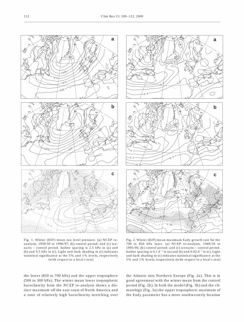
The wintertime MSLP climatology from the NCEP(National Centers for Environmental Prediction) re-analysis (Fig. 1a) shows a minimum of just below1000 hPa between the southern tip of Greenland andIceland and a broad maximum reaching from the At-lantic southwest of the Azores to the Iberian Peninsulaand into Northern Africa. The position and depth of theclimatological Icelandic Low are well reproduced in themodel’s control period (Fig. 1b). The deviation in cen-tral pressure is only about 1 hPa. In contrast, the AzoresHigh is shifted to the northeast and reaches a maximumpressure that is about 5 hPa higher than in the NCEPre-analysis. Consequently, the mean pressure gradientis somewhat higher over Western and Central Europein the simulations than in the re-analysis.
The comparison of the control and the scenarioperiod indicates a strong and statistically significantdecrease (up to 6 hPa) of MSLP at high latitudes in thearea considered (Fig. 1c). Weakly enhanced pressureis found over Southern and Western Europe leading toan increased mean pressure gradient in Northern andCentral Europe and a strengthening of the mean west-erly winds. This signal structure is in good agreementwith the results from a nonlinear trend analysis per-formed by Ulbrich & Christoph (1999) for the samemodel simulation.
Surface cyclone activity and upper air storm trackare related to baroclinic instability, which can be quan-tified in terms of the maximum Eady growth rate (seeEady 1949, Lindzen & Farrell 1980, Hoskins & Valdes1990). It is defined as σBI = 0.31(ƒ/N)|δv/δz|, where ƒ isthe Coriolis parameter, N is the static stability, z is thevertical coordinate and v is the horizontal wind vector.This quantity was calculated from monthly means oftemperature, geopotential height and wind both for
111
Clim Res 15: 109–122, 2000
the lower (850 to 700 hPa) and the upper troposphere(500 to 300 hPa). The winter mean lower troposphericbaroclinicity from the NCEP re-analysis shows a dis-tinct maximum off the east coast of North America anda zone of relatively high baroclinicity stretching over
the Atlantic into Northern Europe (Fig. 2a). This is ingood agreement with the winter mean from the controlperiod (Fig. 2b). In both the model (Fig. 3b) and the cli-matology (Fig. 3a) the upper tropospheric maximum ofthe Eady parameter has a more southwesterly location
112
Fig. 1. Winter (DJF) mean sea level pressure. (a) NCEP re-analysis, 1958/59 to 1996/97; (b) control period; and (c) sce-nario – control period. Isoline spacing is 2.5 hPa in (a) and(b) and 0.5 hPa in (c). Light and dark shading in (c) indicatesstatistical significance at the 5% and 1% levels, respectively
(with respect to a local t-test)
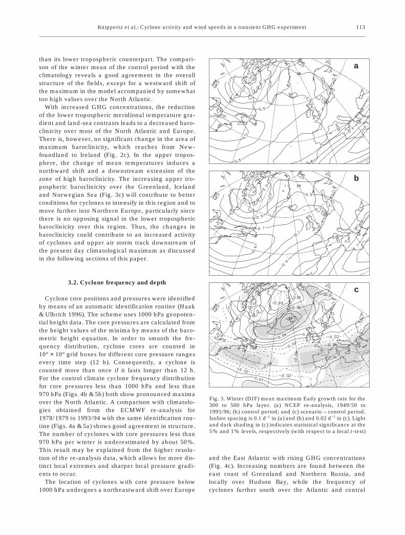
Fig. 2. Winter (DJF) mean maximum Eady growth rate for the700 to 850 hPa layer. (a) NCEP re-analysis, 1949/50 to1995/96; (b) control period; and (c) scenario – control period.Isoline spacing is 0.1 d–1 in (a) and (b) and 0.02 d–1 in (c). Lightand dark shading in (c) indicates statistical significance at the5% and 1% levels, respectively (with respect to a local t-test)
a
b
c
a
b
c
Knippertz et al.: Cyclone activity and wind speeds in a transient GHG experiment
than its lower tropospheric counterpart. The compari-son of the winter mean of the control period with theclimatology reveals a good agreement in the overallstructure of the fields, except for a westward shift ofthe maximum in the model accompanied by somewhattoo high values over the North Atlantic.
With increased GHG concentrations, the reductionof the lower tropospheric meridional temperature gra-dient and land-sea contrasts leads to a decreased baro-clinicity over most of the North Atlantic and Europe.There is, however, no significant change in the area ofmaximum baroclinicity, which reaches from New-foundland to Ireland (Fig. 2c). In the upper tropos-phere, the change of mean temperatures induces anorthward shift and a downstream extension of thezone of high baroclinicity. The increasing upper tro-pospheric baroclinicity over the Greenland, Icelandand Norwegian Sea (Fig. 3c) will contribute to betterconditions for cyclones to intensify in this region and tomove further into Northern Europe, particularly sincethere is no opposing signal in the lower troposphericbaroclinicity over this region. Thus, the changes inbaroclinicity could contribute to an increased activityof cyclones and upper air storm track downstream ofthe present day climatological maximum as discussedin the following sections of this paper.
3.2. Cyclone frequency and depth
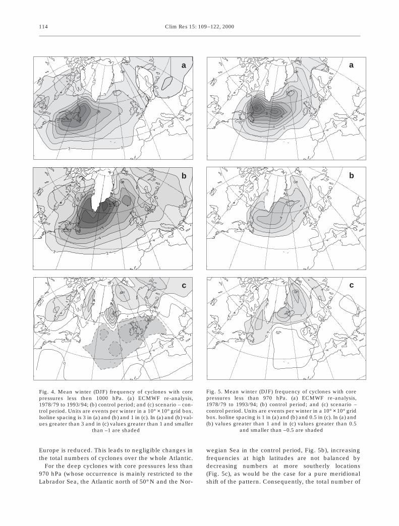
Cyclone core positions and pressures were identifiedby means of an automatic identification routine (Haak& Ulbrich 1996). The scheme uses 1000 hPa geopoten-tial height data. The core pressures are calculated fromthe height values of the minima by means of the baro-metric height equation. In order to smooth the fre-quency distribution, cyclone cores are counted in10° × 10° grid boxes for different core pressure rangesevery time step (12 h). Consequently, a cyclone iscounted more than once if it lasts longer than 12 h.For the control climate cyclone frequency distributionfor core pressures less than 1000 hPa and less than970 hPa (Figs. 4b & 5b) both show pronounced maximaover the North Atlantic. A comparison with climatolo-gies obtained from the ECMWF re-analysis for1978/1979 to 1993/94 with the same identification rou-tine (Figs. 4a & 5a) shows good agreement in structure.The number of cyclones with core pressures less than970 hPa per winter is underestimated by about 50%.This result may be explained from the higher resolu-tion of the re-analysis data, which allows for more dis-tinct local extremes and sharper local pressure gradi-ents to occur.
The location of cyclones with core pressure below1000 hPa undergoes a northeastward shift over Europe
and the East Atlantic with rising GHG concentrations(Fig. 4c). Increasing numbers are found between theeast coast of Greenland and Northern Russia, andlocally over Hudson Bay, while the frequency ofcyclones further south over the Atlantic and central
113
Fig. 3. Winter (DJF) mean maximum Eady growth rate for the300 to 500 hPa layer. (a) NCEP re-analysis, 1949/50 to1995/96; (b) control period; and (c) scenario – control period.Isoline spacing is 0.1 d–1 in (a) and (b) and 0.02 d–1 in (c). Lightand dark shading in (c) indicates statistical significance at the5% and 1% levels, respectively (with respect to a local t-test)
a
b
c
Clim Res 15: 109–122, 2000
Europe is reduced. This leads to negligible changes inthe total numbers of cyclones over the whole Atlantic.
For the deep cyclones with core pressures less than970 hPa (whose occurrence is mainly restricted to theLabrador Sea, the Atlantic north of 50° N and the Nor-
wegian Sea in the control period, Fig. 5b), increasingfrequencies at high latitudes are not balanced bydecreasing numbers at more southerly locations(Fig. 5c), as would be the case for a pure meridionalshift of the pattern. Consequently, the total number of
114
Fig. 4. Mean winter (DJF) frequency of cyclones with corepressures less then 1000 hPa. (a) ECMWF re-analysis,1978/79 to 1993/94; (b) control period; and (c) scenario – con-trol period. Units are events per winter in a 10° × 10° grid box.Isoline spacing is 3 in (a) and (b) and 1 in (c). In (a) and (b) val-ues greater than 3 and in (c) values greater than 1 and smaller
than –1 are shaded
Fig. 5. Mean winter (DJF) frequency of cyclones with corepressures less than 970 hPa. (a) ECMWF re-analysis,1978/79 to 1993/94; (b) control period; and (c) scenario –control period. Units are events per winter in a 10° × 10° gridbox. Isoline spacing is 1 in (a) and (b) and 0.5 in (c). In (a) and(b) values greater than 1 and in (c) values greater than 0.5
and smaller than –0.5 are shaded
a
b
c
a
b
c
Knippertz et al.: Cyclone activity and wind speeds in a transient GHG experiment
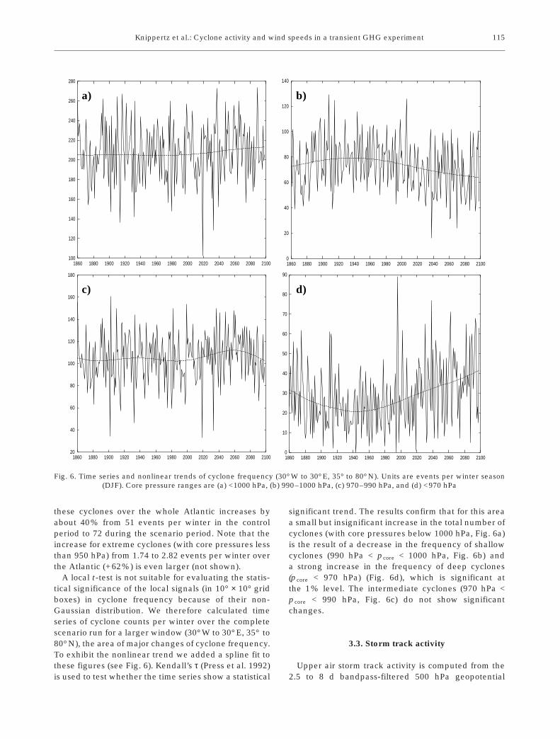
these cyclones over the whole Atlantic increases byabout 40% from 51 events per winter in the controlperiod to 72 during the scenario period. Note that theincrease for extreme cyclones (with core pressures lessthan 950 hPa) from 1.74 to 2.82 events per winter overthe Atlantic (+62%) is even larger (not shown).
A local t-test is not suitable for evaluating the statis-tical significance of the local signals (in 10° × 10° gridboxes) in cyclone frequency because of their non-Gaussian distribution. We therefore calculated timeseries of cyclone counts per winter over the completescenario run for a larger window (30° W to 30° E, 35° to80° N), the area of major changes of cyclone frequency.To exhibit the nonlinear trend we added a spline fit tothese figures (see Fig. 6). Kendall’s τ (Press et al. 1992)is used to test whether the time series show a statistical
significant trend. The results confirm that for this areaa small but insignificant increase in the total number ofcyclones (with core pressures below 1000 hPa, Fig. 6a)is the result of a decrease in the frequency of shallowcyclones (990 hPa < pcore < 1000 hPa, Fig. 6b) anda strong increase in the frequency of deep cyclones(pcore < 970 hPa) (Fig. 6d), which is significant atthe 1% level. The intermediate cyclones (970 hPa <pcore < 990 hPa, Fig. 6c) do not show significantchanges.
3.3. Storm track activity
Upper air storm track activity is computed from the2.5 to 8 d bandpass-filtered 500 hPa geopotential
115
100
120
140
160
180
200
220
240
260
280
1860 1880 1900 1920 1940 1960 1980 2000 2020 2040 2060 2080 2100
a)
0
20
40
60
80
100
120
140
1860 1880 1900 1920 1940 1960 1980 2000 2020 2040 2060 2080 2100
b)
0
10
20
30
40
50
60
70
80
90
1860 1880 1900 1920 1940 1960 1980 2000 2020 2040 2060 2080 2100
d)
20
40
60
80
100
120
140
160
180
1860 1880 1900 1920 1940 1960 1980 2000 2020 2040 2060 2080 2100
c)
Fig. 6. Time series and nonlinear trends of cyclone frequency (30° W to 30° E, 35° to 80° N). Units are events per winter season (DJF). Core pressure ranges are (a) <1000 hPa, (b) 990–1000 hPa, (c) 970–990 hPa, and (d) <970 hPa
Clim Res 15: 109–122, 2000
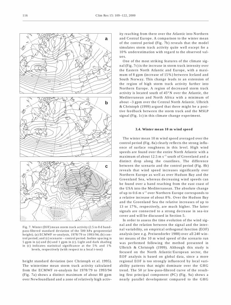
height standard deviation (see Christoph et al. 1995).The wintertime mean storm track activity calculatedfrom the ECMWF re-analysis for 1978/79 to 1993/94(Fig. 7a) shows a distinct maximum of about 80 gpmover Newfoundland and a zone of relatively high activ-
ity reaching from there over the Atlantic into Northernand Central Europe. A comparison to the winter meanof the control period (Fig. 7b) reveals that the modelsimulates storm track activity quite well except for a10% underestimation with regard to the observed val-ues.
One of the most striking features of the climate sig-nal (Fig. 7c) is the increase in storm track intensity overthe Eastern North Atlantic and Europe, with a maxi-mum of 8 gpm (increase of 15%) between Iceland andSouth Norway. This change leads to an extension ofthe region of high storm track activity further intoNorthern Europe. A region of decreased storm trackactivity is located south of 45° N over the Atlantic, theMediterranean and North Africa with a minimum ofabout –3 gpm over the Central North Atlantic. Ulbrich& Christoph (1999) argued that there might be a posi-tive feedback between the storm track and the MSLPsignal (Fig. 1c) in this climate change experiment.
3.4. Winter mean 10 m wind speed
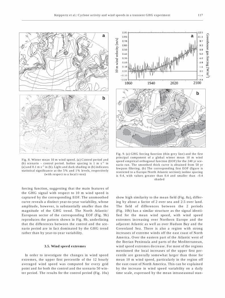
The winter mean 10 m wind speed averaged over thecontrol period (Fig. 8a) clearly reflects the strong influ-ence of surface roughness in this level. High windspeeds are found over the entire North Atlantic with amaximum of about 12.5 m s–1 south of Greenland and adistinct drop along the coastlines. The differencebetween the scenario and the control period (Fig. 8b)reveals that wind speed increases significantly overNorthern Europe as well as over Hudson Bay and theGreenland Sea, whereas decreasing wind speeds canbe found over a band reaching from the east coast ofthe USA into the Mediterranean. The absolute changeof up to 0.6 m s–1 over Northern Europe corresponds toa relative increase of about 8%. Over the Hudson Bayand the Greenland Sea the relative increases of up to13 or 17%, respectively, are much higher. The lattersignals are connected to a strong decrease in sea-icecover and will be discussed in Section 5.
In order to assess the time evolution of the wind sig-nal and the relation between the signal and the inter-nal variability, an empirical orthogonal function (EOF)analysis (see e.g. Preisendorfer 1988) over all 240 win-ter means of the 10 m wind speed of the scenario runwas performed following the method presented inUlbrich & Christoph (1999). Although this study isfocused on the North Atlantic/European sector, theEOF analysis is based on global data, since a moreregional EOF is too strongly influenced by local vari-ability patterns that might dominate over the GHGtrend. The 50 yr low-pass-filtered curve of the result-ing first principal component (PC) (Fig. 9a) shows anearly parallel development compared to the GHG
116
Fig. 7. Winter (DJF) mean storm track activity (2.5 to 8 d band-pass-filtered standard deviation of the 500 hPa geopotentialheight). (a) ECMWF re-analysis, 1978/79 to 1993/94; (b) con-trol period; and (c) scenario – control period. Isoline spacing is5 gpm in (a) and (b) and 1 gpm in (c). Light and dark shadingin (c) indicates statistical significance at the 5% and 1%
levels, respectively (with respect to a local t-test)
a
b
c
Knippertz et al.: Cyclone activity and wind speeds in a transient GHG experiment
forcing function, suggesting that the main features ofthe GHG signal with respect to 10 m wind speed iscaptured by the corresponding EOF. The unsmoothedcurve reveals a distinct year-to-year variability, whoseamplitude, however, is substantially smaller than themagnitude of the GHG trend. The North Atlantic/European sector of the corresponding EOF (Fig. 9b)reproduces the pattern shown in Fig. 8b, underliningthat the differences between the control and the sce-nario period are in fact dominated by the GHG trendrather than by year-to-year variability.
3.5. Wind speed extremes
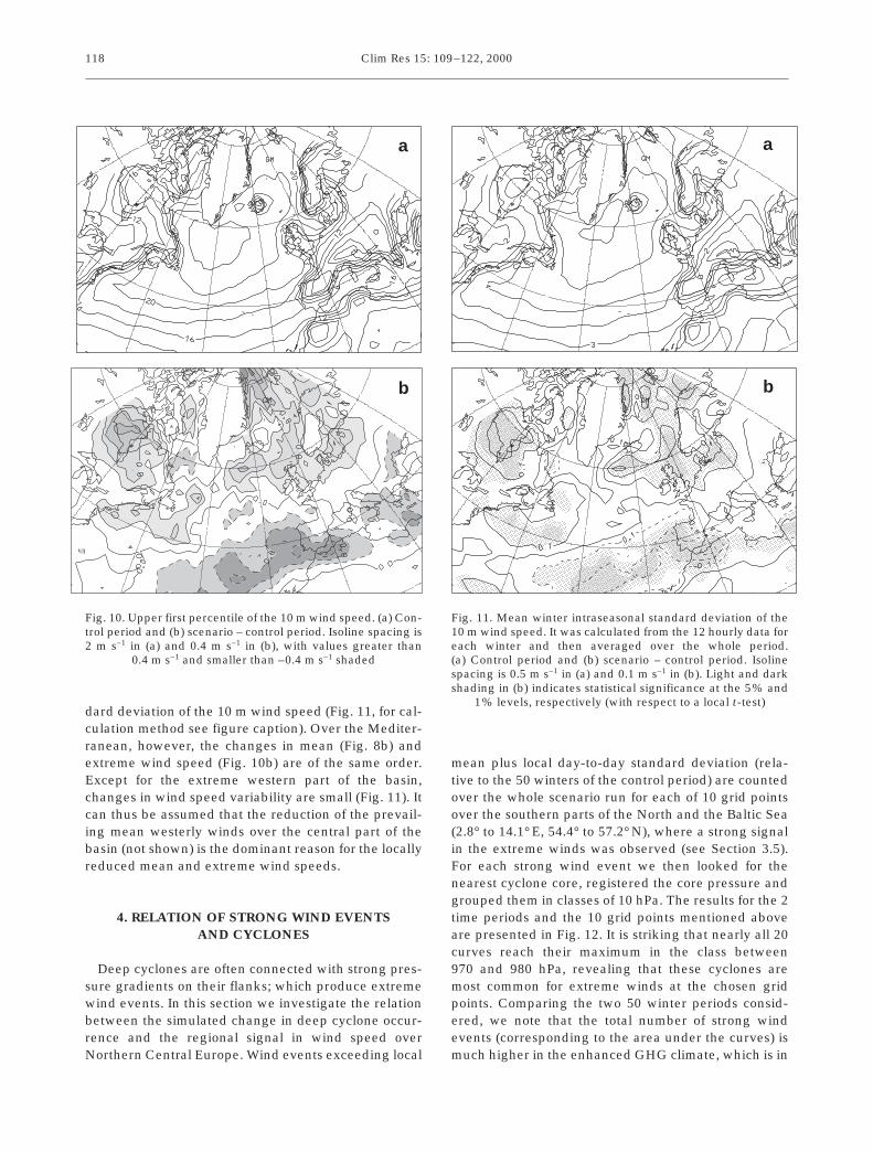
In order to investigate the changes in wind speedextremes, the upper first percentile of the 12 hourlyaveraged wind speed was computed for every gridpoint and for both the control and the scenario 50 win-ter period. The results for the control period (Fig. 10a)
show high similarity to the mean field (Fig. 8a), differ-ing by about a factor of 2 over sea and 2.5 over land.The field of differences between the 2 periods(Fig. 10b) has a similar structure as the signal identi-fied for the mean wind speed, with wind speedextremes increasing over Northern Europe and theadjacent Atlantic as well as over Hudson Bay and theGreenland Sea. There is also a region with strongincreases of extreme winds off the east coast of NorthAmerica. Over the eastern part of the Atlantic west ofthe Iberian Peninsula and parts of the Mediterranean,wind speed extremes decrease. For most of the regionsmentioned the local increases of the upper first per-centile are generally somewhat larger than those formean 10 m wind speed, particularly in the region offthe east coast of North America. This can be explainedby the increase in wind speed variability on a dailytime scale, expressed by the mean intraseasonal stan-
117
Fig. 8. Winter mean 10 m wind speed. (a) Control period and(b) scenario – control period. Isoline spacing is 1 m s–1 in(a) and 0.1 m s–1 in (b). Light and dark shading in (b) indicatesstatistical significance at the 5% and 1% levels, respectively
(with respect to a local t-test)
Greenhouse gas forcing [W
/m2]
1860 1940 2020 2100
10 m
win
d ve
loci
ty [
m/s
]
Fig. 9. (a) GHG forcing function (thin grey line) and the firstprincipal component of a global winter mean 10 m windspeed empirical orthogonal function (EOF) for the 240 yr sce-nario run. The smoothed thick curve is obtained from 50 yrlowpass filtering. (b) The corresponding first EOF (figure isrestricted to a Europe/North Atlantic section); isoline spacingis 0.4, with values greater than 0.4 and smaller than –0.4
shaded
a
b
a
b
Clim Res 15: 109–122, 2000
dard deviation of the 10 m wind speed (Fig. 11, for cal-culation method see figure caption). Over the Mediter-ranean, however, the changes in mean (Fig. 8b) andextreme wind speed (Fig. 10b) are of the same order.Except for the extreme western part of the basin,changes in wind speed variability are small (Fig. 11). Itcan thus be assumed that the reduction of the prevail-ing mean westerly winds over the central part of thebasin (not shown) is the dominant reason for the locallyreduced mean and extreme wind speeds.
4. RELATION OF STRONG WIND EVENTS AND CYCLONES
Deep cyclones are often connected with strong pres-sure gradients on their flanks; which produce extremewind events. In this section we investigate the relationbetween the simulated change in deep cyclone occur-rence and the regional signal in wind speed overNorthern Central Europe. Wind events exceeding local
mean plus local day-to-day standard deviation (rela-tive to the 50 winters of the control period) are countedover the whole scenario run for each of 10 grid pointsover the southern parts of the North and the Baltic Sea(2.8° to 14.1° E, 54.4° to 57.2° N), where a strong signalin the extreme winds was observed (see Section 3.5).For each strong wind event we then looked for thenearest cyclone core, registered the core pressure andgrouped them in classes of 10 hPa. The results for the 2time periods and the 10 grid points mentioned aboveare presented in Fig. 12. It is striking that nearly all 20curves reach their maximum in the class between970 and 980 hPa, revealing that these cyclones aremost common for extreme winds at the chosen gridpoints. Comparing the two 50 winter periods consid-ered, we note that the total number of strong windevents (corresponding to the area under the curves) ismuch higher in the enhanced GHG climate, which is in
118
Fig. 10. Upper first percentile of the 10 m wind speed. (a) Con-trol period and (b) scenario – control period. Isoline spacing is2 m s–1 in (a) and 0.4 m s–1 in (b), with values greater than
0.4 m s–1 and smaller than –0.4 m s–1 shaded
Fig. 11. Mean winter intraseasonal standard deviation of the10 m wind speed. It was calculated from the 12 hourly data foreach winter and then averaged over the whole period.(a) Control period and (b) scenario – control period. Isolinespacing is 0.5 m s–1 in (a) and 0.1 m s–1 in (b). Light and darkshading in (b) indicates statistical significance at the 5% and
1% levels, respectively (with respect to a local t-test)
a
b
a
b
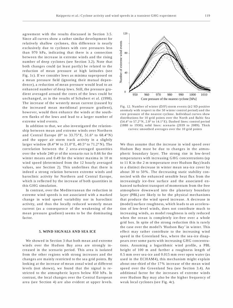
Knippertz et al.: Cyclone activity and wind speeds in a transient GHG experiment
agreement with the results discussed in Section 3.5.Since all curves show a rather similar development forrelatively shallow cyclones, this difference is nearlyexclusively due to cyclones with core pressures lessthan 970 hPa, indicating that there is a connectionbetween the increase in extreme winds and the risingnumber of deep cyclones (see Section 3.2). Note thatboth changes could (at least partly) be related to thereduction of mean pressure at high latitudes (seeFig. 1c). If we consider lows as minima superposed ona mean pressure field (ignoring their mutual depen-dence), a reduction of mean pressure would lead to anenhanced number of deep lows. Still, the pressure gra-dient averaged around the cores of the lows could beunchanged, as in the results of Schubert et al. (1998).The increase of the westerly mean current (caused bythe increased mean meridional pressure gradient),however, would then enhance the winds at the south-ern flanks of the lows and lead to a larger number ofextreme wind events.
In addition to that, we also investigated the relation-ship between mean and extreme winds over Northernand Central Europe (0° to 33.75° E, 51.6° to 68.4° N)and the upper air storm track activity in a slightlylarger window (8.4° W to 31.0° E, 40.5° to 71.2° N). Thecorrelation between the 2 area-averaged quantitiesover the whole 240 yr of the scenario run is 0.66 for thewinter means and 0.49 for the winter maxima in 10 mwind speed (determined from the 12 hourly averagedvalues, see Section 2). This underlines that there isindeed a strong relation between extreme winds andbaroclinic activity for Northern and Central Europe,which is reflected by the increase of both quantities inthis GHG simulation.
In contrast, over the Mediterranean the reduction inextreme wind speeds is not associated with a markedchange in wind speed variability nor in baroclinicactivity, and thus the locally reduced westerly meancurrent (as a consequence of the weakening of themean pressure gradient) seems to be the dominatingfactor.
5. WIND SIGNALS AND SEA ICE
We showed in Section 3 that both mean and extremewinds over the Hudson Bay area are strongly in-creased in the scenario period. This area is isolatedfrom the other regions with strong increases and thechanges are mainly restricted to the sea grid points. Bylooking at the increase of mean zonal wind at differentlevels (not shown), we found that the signal is re-stricted to the atmospheric layers below 850 hPa. Incontrast, the local changes over the Central Europeanarea (see Section 4) are also evident at upper levels.
We thus assume that the increase in wind speed overHudson Bay must be due to changes in the atmos-pheric boundary layer. The strong rise in low-leveltemperatures with increasing GHG concentrations (upto 11 K in the 2 m temperature over Hudson Bay) leadsto a distinct decrease in winter mean sea-ice cover byabout 30 to 50%. The decreasing static stability con-nected with the enhanced sensible heat flux from theincreasingly ice-free surface and the associated en-hanced turbulent transport of momentum from the freeatmosphere downward into the planetary boundarylayer (PBL) are likely to be the physical mechanismsthat produce the wind speed increase. A decrease in(model) surface roughness, which leads to an accelera-tion of low-level winds, does not contribute much toincreasing winds, as model roughness is only reducedwhen the ocean is completely ice-free over a wholegrid box. In spite of the strong reduction this is rarelythe case over the model’s ‘Hudson Bay’ in winter. Thiseffect may rather contribute to the increasing windspeed in the Greenland Sea, where the sea-ice disap-pears over some parts with increasing GHG concentra-tions. Assuming a logarithmic wind profile, a PBLheight of 100 m and further a roughness length of0.5 mm over sea-ice and 0.015 mm over open water (asused in the ECHAM4), this mechanism might explainabout one-third of the 17% increase of the mean windspeed over the Greenland Sea (see Section 3.4). Anadditional factor for the increases of extreme windsover Hudson Bay may also be the higher frequency ofweak local cyclones (see Fig. 4c).
119
0
20
40
60
80
100
120
Core pressure of the nearest cyclone [hPa]960 980 1000 1010990970950
Num
ber
of e
xtre
me
win
d ev
ents
0
40
80
120
Fig. 12. Number of winter (DJF) storm events (≥2 SD positiveanomaly with respect to the 50 winter control period) and thecore pressure of the nearest cyclone. Individual curves showdistributions for 10 grid points over the North and Baltic Sea(54.4° to 57.2° N, 2.8° to 14.1° E). Dashed lines: control period(1880 to 1930); solid lines: scenario (2039 to 2089). Thick
curves: smoothed averages over the 10 grid points
Clim Res 15: 109–122, 2000
6. DISCUSSION AND CONCLUSIONS
Synoptic activity and 10 m wind speed over Europe,the North Atlantic and Eastern North America areanalysed in a 240 yr transient GHG forcing experiment(according to the IS92a scenario) with the ECHAM4/OPYC3 coupled ocean-atmosphere model at T42 reso-lution. In summary, the most important changes underthe GHG forcing simulated by the model are the follo-ing: (1) The position of the cyclone cores is shiftednorth- and eastward over Europe and the EasternNorth Atlantic. (2) The number of relatively shallowcyclones over Europe and the Eastern North Atlanticdecreases slightly. The number of deep cyclonesincreases, so that the total number of cyclones changesonly insignificantly. (3) Over the Hudson Bay and theGreenland Sea both mean wind speeds and windspeed extremes increase caused by changes in the PBLdue to a strong decrease in winter mean sea-ice cover.Over Northern Europe and parts of the Eastern NorthAtlantic the positive signal in mean and extreme windspeed is caused by an intensification of the westerlymean current and an augmented occurrence of deepcyclones. Over the Mediterranean, where small changesin cyclone frequency were found, decreasing meanand extreme wind speeds are associated with a weak-ening of the westerly mean current.
The climate signals of MSLP, low-level wind, synop-tic activity and baroclinicity have been shown to beconsistent with each other. The assignment of thechanges to the climate signal rather than long-termvariability was shown for 10 m wind velocities on thebasis of an EOF analysis. The same had been done byUlbrich & Christoph (1999) with respect to storm trackactivity and sea-level pressure for the same model run.There is a close relationship between the cyclone sig-nal and the signal in the 500 hPa storm track. On theone hand both parameters undergo a northeastwardshift over the Eastern North Atlantic and Europe, andon the other hand the intensification of the storm trackactivity over the north of this region can probably beassociated with the augmented occurrence of deepcyclones. Furthermore, the changes in storm trackactivity are in good agreement with the signal inupper-tropospheric baroclinicity, which is locatedupstream of the storm track signal, indicating that theadditional baroclinicity supports the intensification ofdeveloping synoptic systems in this region.
Our results agree with many other GCM studies onGHG forcing. This statement refers to the northwardshift of the cyclone tracks and the upper air storm trackactivity over Europe and the North Atlantic (König etal. 1993, Hall et al. 1994, Schubert et al. 1998), and tothe increased number of deep and the decreased num-ber of shallow cyclones with increasing GHG concen-
trations over this region (Lambert 1995, Carnell &Senior 1998). With respect to the storm track over theNortheast Atlantic, an enhancement is also common tomany model studies (see also Hall et al. 1994, Lunkeitet al. 1996, Cubasch et al. 1997, Schubert et al. 1998).In agreement with our findings, an increasing occur-rence of high wind speeds over the East Atlantic andEurope has been found by Lunkeit et al. (1996) and byCarnell et al. (1996). Corresponding to the findings ofZwiers & Kharin (1998), we find larger wind extremesin the areas where sea-ice retreated. The coincidenceof results from quite different model configuration maypoint to some degree of robustness and reliability. Aninvestigation with an ECHAM4/T106 time-slice exper-iment revealed that the results of this study are alsolargely insensitive with respect to changes in themodel’s horizontal resolution (W. May, Danish Meteo-rological Institute, pers. comm. 1999). Some of thestudies whose results do not agree with ours are basedon very short time slices (e.g. Beersma et al. 1997) or onmodel simulations which have some problems repro-ducing the observed patterns of baroclinic activity(Zhang & Wang 1997).
The GHG run considered here does not take intoaccount the effects of anthropogenic changes in sul-phur aerosols. Transient climate change experimentsincluding these effects show that in winter the coolingdue to aerosols merely leads to a reduction of the tem-perature response to carbon dioxide (Mitchell & Johns1997, Roeckner et al. 1998). One may expect that theclimate signal in the synoptic activity is also weakenedby this additional effect. It is still important to performthe climate change investigations with GHG forcingonly. A sensitivity experiment with the HadCM2 modelrevealed that the weakening influence of sulphuraerosols on GHG induced global temperature rise van-ishes within 1 decade after their removal during thecontinuing transient simulation (T. Johns, Hadley Cen-tre, pers. comm. 1999).
We would like to emphasize that, in spite of a certainagreement between different models, considerable in-security about their results remains. While some of themechanisms leading to the changes are evident (theincrease in upper air baroclinicity, increasing latentheat release within the baroclinic waves adding totheir energy, see Hoffmann 1999 and Cubasch et al.1999), the apparently most important effect, the in-creasing number of deep cyclones at the cost of shallowcyclones, has to be carefully investigated in order toexclude the possibility of an artifact of the GCMs. It isnot clear whether secondary lows or short-wave distur-bances and their importance for the generation of ex-treme wind events are simulated realistically enough.
Another problem regarding the interpretation of cli-mate change studies arises from the resolution of cli-
120
Knippertz et al.: Cyclone activity and wind speeds in a transient GHG experiment
mate models, which affects the representation of orog-raphy, the land-sea distribution, etc., and consequentlythe wind signal. We will have to wait for improvementsin the nesting of high resolution regional models inorder to obtain a more reliable estimate of the localimpacts of climate change with respect to extremewind events.
Acknowledgements. We would like to thank the anonymousreviewers for their detailed comments that helped to improvethe manuscript. This work was partially supported by theDeutsche Forschungsgemeinschaft within Sonderforschungs-bereich (SFB) 419 and by the Federal German Ministry ofResearch (BMBF) under grant No. 01 LA9861/5.
LITERATURE CITED
Bacher A, Oberhuber MJ, Roeckner E (1998) ENSO dynamicsand seasonal cycle in the tropical Pacific as simulated bythe ECHAM4/OPYC3 coupled general circulation model.Clim Dyn 14:431–450
Beersma JJ, Rider KM, Komen GJ, Kaas E, Kharin VV (1997)An analysis of extra-tropical storms in the North Atlanticregion as simulated in a control and 2 × CO2 time-sliceexperiment with a high-resolution atmospheric model.Tellus 49A:347–361
Carnell RE, Senior CA (1998) Changes in mid-latitude vari-ability due to increasing greenhouse gases and sulphateaerosols. Clim Dyn 14:369–383
Carnell RE, Senior CA, Mitchell JFB (1996) An assessment ofmeasures of storminess: simulated changes in northernhemisphere winter due to increasing CO2. Clim Dyn 12:467–476
Christoph M, Ulbrich U, Haak U (1995) Faster determinationof the intraseasonal variability of storm tracks using Mura-kami’s recursive filter. Mon Weather Rev 122:578–581
Cubasch U (ed), Caneill JY, Filiberti MA, Hegerl G, Johns TC,Keen A, Parey S, Thual O, Ulbrich U, Voss R, WaszkewitzJ, Wild M, van Ypersele JP (1997) Anthropogenic climatechange. Project No. EV5V-CT92–0123 final report. Officefor Official Publications of the European Comission No.EUR 17466EN, Luxembourg
Cubasch U, Allen M, Beniston M, Bertrand C, Brinkop S,Caneill JY, Dufresne JL, Fairhead L, Filiberti MA, GregoryJ, Hegerl G, Hoffmann G, Johns T, Jones G, Laurent C,McDonald R, Mitchell J, Parker D, Oberhuber J, Poncin C,Sausen R, Schlese U, Stott P, Tett S, leTreut H, Ulbrich U,Valcke S, Voss R, Wild M, Ypersele JP (1999) SummaryReport of the Project Simulation, Diagnosis and Detectionof the Anthropogenic Climate Change (SIDDACLICH).ENV4-CT95–0102. Office for Official Publications of theEuropean Commission No. EUR 19310, Luxembourg
Dorland C, Tol RSJ, Olsthoorn AA, Palutikof JP (1996) Ananalysis of storm impacts in the Netherlands. In: DowningTE, Olsthoorn AA, Tol RSJ (eds) Climatic change andextreme events. ECU-Research Report Number 12, VUBoekhandel/Uitgeverij, Amsterdam, p 157–184
Dronia H (1991) On the accumulation of excessive low pres-sure systems over the North Atlantic during the winterseasons (November to March) 1988/89 to 1990/91. DieWitterung in Übersee 39:27
Eady ET (1949) Long waves and cyclone waves. Tellus 1:33–52
Fantini M (1993) A numerical study of two-dimensional moistbaroclinic instability. J Atmos Sci 50:1199–1210
Golding B (1984) A study of the structure of mid-latitudedepressions in a numerical model using trajectory tech-niques. I: Development of ideal baroclinic waves in dryand moist atmospheres. Q J R Meteorol Soc 110:847–879
Gutowski WJ, Branscome LE, Stewart DA (1992) Life cycles ofmoist baroclinic eddies. J Atmos Sci 49:306–319
Haak U, Ulbrich U (1996) Verification of an objective cycloneclimatology for the North Atlantic. Meteorol Z 5:24–30
Hall NMJ, Hoskins BJ, Valdes PJ, Senior CA (1994) Stormtracks in a high-resolution GCM with doubled carbondioxide. Q J R Meteorol Soc 120:1209–1230
Held IM (1993) Large scale dynamics and global warming.Bull Am Meteorol Soc 74:228–241
Held IM, O’Brien EO (1992) Quasigeostrophic turbulence in aThree-Layer-Model: effects of vertical structure in themean shear. J Atmos Sci 49:1861–1870
Hoffmann G (1999) Die Bedeutung der diabatischen Heizungfür die synoptische Störungsaktivität der Nordhemisphäreim heutigen und in einem zukünftigen Klima. In: Ebel A,Kerschgens M, Neubauer FM, Speth P (eds) Mitteilungenaus dem Institut für Geophysik und Meteorologie der Uni-versität zu Köln. University of Cologne
Hoskins BJ, Valdes PJ (1990) On the existence of storm-tracks. J Atmos Sci 47:1854–1864
IPCC (1992) Climate change 1992: the supplementary reportto the IPCC scientific assessment. Cambridge UniversityPress, Cambridge
IPCC (1996) Climate change 1995: the science of climatechange. Cambridge University Press, Cambridge
Kaas E, Li TS, Schmith T (1996) Statistical hindcast of windclimatology in the North Atlantic and northwestern Euro-pean region. Clim Res 7:97–110
Karoly DJ, Cohen JA, Meehl GA, Mitchell JFB, Oort AH,Stouffer RJ, Wetherald RT (1994) An example of finger-print detection of greenhouse climate change. Clim Dyn10:97–105
König W, Sausen R, Sielmann F (1993) Objective identifica-tion of cyclones in GCM simulations. J Clim 6:2217–2231
Lambert SJ (1995) The effect of enhanced greenhouse warm-ing on winter cyclone frequencies and strength. J Clim 8:1447–1452
Lambert SJ (1996) Intense extratropical Northern Hemi-sphere winter cyclone events: 1899–1991. J Geophys Res101:21319–21325
Lindzen RS, Farrel B (1980) A simple approximate result forthe maximum growth rate of baroclinic instabilities.J Atmos Sci 37:1648–1654
Lunkeit F, Ponater M, Sausen R, Sogalla M, Ulbrich U,Windelband M (1996) Cyclonic activity in a warmer cli-mate. Beitr Phys Atmos 69:393–407
Lunkeit F, Fraedrich K, Bauer SE (1998) Storm tracks in awarmer climate: sensitivity studies with a simplified globalcirculation model. Clim Dyn 14:813–826
Machenhauer B, Windelband M, Botzet M, Hesselbjerg-Christensen J, Deque M, Jones RG, Ruti PM, Visconti G(1998) Validation and analysis of regional present-dayclimate and climate-change simulations over Europe.Report No. 275, Max-Planck-Institut für Meteorologie,Hamburg
Mengelkamp HT (1999) Wind climate simulation over com-plex terrain and wind turbine energy output estimation.Theor Appl Climatol 63:129–139
Mitchell JFB, Johns TC (1997) On the modification of globalwarming by sulphate aerosols. J Clim 10:245–267
Mitchell JFB, Manabe S, Tokioka T, Meleshko V (1990) Equi-
121
Clim Res 15: 109–122, 2000
librium climate change. In: Houghton JT, Jankins GJ,Ephraums JJ (eds) Climate change, the IPCC scientificassessment. Cambridge University Press, Cambridge,p 131–172
Munich Re (1977) Der Capella-Orkan. Januarstürme 1976über Europa. Münchener Rückversicherungs-Gesellschaft
Munich Re (1990) Sturm—Neue Schadendimensionen einerNaturgefahr. Münchener Rückversicherungs-Gesellschaft
Oberhuber JM (1993) Simulation of the Atlantic circulationwith a coupled sea ice-mixed layer-isopycnal general cir-culation model. Part I: Model description. J Phys Oceanogr22:808–829
Pavan V (1996) Sensitivity of a multi-layer, quasi-geostrophicβ-channel to the vertical structure of the equilibriummeridional temperature gradient. Q J R Meteorol Soc 122:55–72
Penning-Rowsell E, Handmer J, Tapsell S (1996) An analysisof storm impacts in the Netherlands. In: Downing TE,Olsthoorn AA, Tol RSJ (eds) Climatic change and extremeevents. ECU-Research Report Number 12, VU Boekhan-del/Uitgeverij, Amsterdam, p 97–127
Preisendorfer RW (1988) Principal component analysis inmeteorology and oceanography. In: Mobley CD (ed)Developments in atmospheric science, Vol 17. Elsevier,Amsterdam
Press WH, Teukolsky SA, Netterling WT, Flannery BP (eds)(1992) Numerical recipes in FORTRAN, 2nd edn. Cam-bridge University Press, Cambridge, p 488–494
Roeckner E, Arpe K, Bengtsson L, Dümenil L, Esch M, Kirk E,Lunkeit F, Ponater M, Rockel B, Sausen R, Schlese U,Schubert S, Windelband M (1992) Simulation of present-day climate with the ECHAM model: impact of modelphysics and resolution. Report No. 93, Max-Planck-Institutfür Meteorologie, Hamburg
Roeckner E, Arpe K, Bengtsson L, Christof M, Claussen M,Dümenil L, Esch M, Giorgetta M, Schlese U, SchulzweidaU (1996a) The atmospheric general circulation modelECHAM4: model description and simulation of present-day climate. Report No. 218, Max-Planck-Institut fürMeteorologie, Hamburg
Roeckner E, Oberhuber JM, Bacher A, Christof M, Kirchner I
(1996b) ENSO variability and atmospheric response in aglobal coupled atmosphere-ocean GCM. Clim Dyn 12:737–754
Roeckner E, Bengtsson L, Feichter J, Lelieveld J, Rhode H(1998) Transient climate change simulations with a cou-pled atmosphere-ocean GCM including the troposphericsulfur cycle. Report No. 266, Max-Planck-Institut fürMeteorologie, Hamburg
Schinke H (1993) On the occurrence of deep cyclones overEurope and the North Atlantic in the period 1930–1991.Beitr Phys Atmos 66:223–237
Schmith T, Kaas E, Li TS (1998) Northeast Atlantic winterstorminess 1875–1995 re-analysed. Clim Dyn 14:529–536
Schraft A, Durand E, Hausmann P (1993) Storms over Europe:losses and scenarios. Swiss Reinsurance Company, Zürich
Schubert M, Perlwitz J, Blender R, Fraedrich K, Lunkeit F(1998) North Atlantic cyclones in CO2-induced warm cli-mate simulations: frequency, intensity and tracks. ClimDyn 14:827–837
Stein O, Hense A (1994) A reconstructed time series of thenumber of extreme low pressure events since 1880. Mete-orol Z NF 3:43–46
Stephenson DB, Held IM (1993) GCM response of northernwinter stationary waves and storm tracks to increasingamounts of carbon dioxide. J Clim 6:1859–1870
Ulbrich U, Christoph M (1999) A shift of the NAO and increas-ing storm track activity over Europe due to anthropogenicgreenhouse gas forcing. Clim Dyn 15:551–559
von Storch H, Guddal J, Iden KA, Jonsson T, Perlwitz J, Reis-tad M, de Ronde J, Schmidt H, Zorita E (1993) Changingstatistics of storms in the North Atlantic? Report No. 116,Max-Planck-Institut für Meteorologie, Hamburg
WASA-Group (Waves and Storms in the North Atlantic)(1998) Changing waves and storms in the NortheastAtlantic. Bull Am Meteorol Soc 79:741–760
Zhang Y, Wang WC (1997) Model-simulated northern wintercyclone an anticyclone activity under a greenhouse warm-ing scenario. J Clim 10:1616–1634
Zwiers FW, Kharin VV (1998) Changes in the extremes of theclimate simulated by the CCC GCM2 under CO2 dou-bling. J Clim 11:2200–2222
122
Editorial responsibility: Hans von Storch,Geesthacht, Germany
Submitted: October 7, 1999; Accepted: January 24, 2000Proofs received from author(s): May 22, 2000