Changes in the Global Oil Market

Erdenebat Bataa

National University of Mongolia & Ministry of Finance, Mongolia

Marwan Izzeldin

University of Lancaster

Denise R.Osborn∗

University of Manchester & University of Tasmania

March 2016

Abstract

Changes in the parameters of a recursively identified oil market model are examined through

an iterative algorithm that tests for possible breaks in coefficients and variances. The analy-

sis detects breaks in the coefficients of the oil production and price equations, together with

volatility shifts in all three equations of the model. Coefficient changes imply an enhanced

response of production to aggregate demand shocks after 1980; and that the price response

to supply shocks is more persistent from the mid-1990s. All variables evidence changes in

the relative contributions of individual shocks to their forecast error variances, with coeffi-

cient and volatility breaks in the first half of the 1990s being particularly important in this

respect. The results show that analysts of this market should eschew constant parameter

models estimated over an extended period.

JEL classification: E42, Q43.

Keywords: Oil price shocks, multiple breaks, breaks in SVAR

∗Corresponding author. Denise Osborn, Centre for Growth and Business Cycles Research, Eco-nomics, School of Social Sciences, University of Manchester, Oxford Road, Manchester, UK, M13 9PL,denise.osborn@manchester.ac.uk. Erdenebat Bataa, Department of Economics, National University of Mongo-lia, Baga Toiruu 4, Ulaanbaatar, Mongolia, tsors79@yahoo.com. Marwan Izzeldin, Department of Economics,Lancaster University Management School, Lancaster, UK, LA1 4YW, m.izzeldin@lancaster.ac.uk.Acknowledgements: We would like to thank Lutz Kilian and Pierre Perron for making their datasets and computerprograms available on the Internet, the modifications of which were used in this paper. We are also grateful toseminar and conference participants at the 2015 Royal Economic Society Conference, Lancaster University, Uni-versity of Manchester, National University of Mongolia, Korea University, Open Society Institute AFP Meeting,OxMetrics conference, and Yonsei Global Research Team Workshop for their constructive comments. Finally, theauthors would like to thank two referees of this journal, whose helpful comments have improved the exposition ofthis paper.

1

1 Introduction

A growing literature has underlined the importance of distinguishing between demand and supply

shocks in the global oil market. In particular, the seminal paper of Kilian (2009) argues that

traditional vector autoregressive (VAR) modeling methodologies do not separate these shocks and

hence an increase in the price of oil following an expansion in the level of global economic activity

could be wrongly attributed as an oil price shock. To avoid this problem, Kilian (2009) proposes

ordering restrictions to define a structural VAR (SVAR) model that captures the essential features

of the world oil market and, consequently, disentangles demand and supply shocks.

Nevertheless, the nature of the oil market has changed over the four decades following the

oil price shocks of the mid-1970s. The transition from the ‘official price’ regime of the earlier

period, when the oil price was set by long-term contracts, to the current market-based system

of direct trading in spot and futures markets, has seen the power balance shift away from the

Organization of the Petroleum Exporting Countries (OPEC); see Mabro (2006) for a detailed

account of the changes in pricing regimes. Moreover, OPEC itself experienced internal structural

instability, leading to its near-collapse in 1986, while the new millennium saw an oil price boom

and an important role played by emerging economies (Hamilton, 2014, Kilian and Hicks, 2013,

Kilian and Lee, 2014), but a very recent price collapse. These considerations suggest change

may apply in the parameters of oil market SVAR models since the 1970s. The present paper

examines this question through a model adopting the identifying restrictions proposed by Kilian

(2009) to which recently developed structural break tests are applied.

The analysis of Kilian (2009), together with many subsequent studies (including Kilian and

Murphy, 2014, Kilian and Park, 2009), assumes the model parameters are constant over time.

However, if the parameters change then false conclusions may be drawn about both the past and,

more importantly, the contemporary consequences of oil shocks. That is, analysis through the

conventional SVAR tools of impulse response analysis and forecast error variance decompositions

can be seriously misleading if constant parameters are assumed when, in fact, the parameters

have changed over the period used for estimation.

Despite the predominant assumption of constant parameters, some authors have recognised

the potential importance of change in oil market models. For example, both Sadorsky (1999) and

Peersman and Van Robays (2012) assume change occurs at the end of 1985, whereas Baumeister

and Peersman (2013b) employ a time-varying parameter SVAR (TVP-SVAR) specification that

implies continuous evolution in all parameters. Lutkepohl and Netsunajev (2014), on the other

hand, apply a Markov switching model for the volatility of oil market shocks in a specification

with other parameters constant. Our formal structural breaks analysis provides complementary

information to these studies, allowing for discrete breaks of unknown number and, in particular,

permitting the null hypothesis of no change to be explicitly considered. A discrete break test of

the type that we use is known to have power against other alternatives, such as one in which the

coefficients follow a random walk (see Stock and Watson, 1998 and Boivin and Giannoni, 2006).

While the continuous change implied by the random walk assumption (used by Baumeister and

2

Peersman, 2013b) is flexible in modelling terms, it results in a loss of estimation accuracy if

employed in a period of constant coefficients.

To the best of our knowledge, the present paper is the first to apply formal statistical tests

to examine the existence and nature of change in both the structural coefficients and the shock

volatilities of an oil market model. In other words, rather than assuming either constant param-

eters or change at specific dates, we ‘let the data speak’. Further, since parameters are constant

in our model within regimes, we are able to construct conventional confidence intervals for im-

pulse response functions and forecast error variance decompositions, whereas these tools have

limited applicability in a model with continuous change. For these reasons, we prefer to test

for parameter change (or structural breaks), rather than impose either continuous change or to

(perhaps arbitrarily and potentially incorrectly) pre-specify the date or dates at which change

may occur.

An important implication of the analysis of Baumeister and Peersman (2013b) is that changes

in coefficients and the volatilities of shocks in this market may apply at different dates, and we

allow for this through the testing approach of Bataa, Osborn, Sensier and van Dijk (2013).

However, the latter applies to a conventional VAR model, so the methodology is here extended

to the recursively ordered SVAR context. In particular, by considering each equation separately,

our methodology not only permits coefficients and volatilities to change at different dates, but

dates of change may also differ over equations. Prior to estimation, the respective null hypotheses

of no change are explicitly examined for coefficients and volatility in each equation. Although

our focus is the world oil market, the structural break testing methodology developed here can

be used within any recursively ordered SVAR model.

Our results confirm that both the SVAR coefficients and the volatilities of shocks have changed

over the four decades to early 2014, so that constant parameter modelling is not appropriate.

Further, these changes have important implications for understanding the world oil market.

More specifically, coefficient changes are found in the oil production equation at the end of

1980, with supply shocks having a transient effect on production before that date but permanent

effects subsequently. On the other hand, breaks are found in the oil price equation in 1988

and 1994, with the post-1994 period showing distinct responses compared with earlier sub-

periods. Indeed, only this latest period (1994 to 2014) shows positive price responses to negative

supply shocks at all horizons and it also exhibits substantially faster price responses to oil-

specific demand shocks. Therefore, predictions based on a model not allowing for change would

substantially underestimate the responsiveness of the oil price to both supply and demand shocks.

Interestingly, the global financial crisis (GFC) and other events of the new millennium do not

appear to have altered the coefficients of these relationships.

Further, volatility changes are uncovered in all three equations, but the only volatility break

apparently associated with the onset of the GFC occurs in the economic activity equation.

Volatility as well as coefficient changes over the period are shown to have important effects on

the forecast error variance decompositions, with oil supply shocks contributing less and oil specific

3

demand shocks more for all variables over the second half of our sample period. In particular,

whereas supply shocks were the most important contributor to oil price inflation volatility two

or more years ahead in the period to the mid-1980s, the dominant role has been played by oil-

specific demand shocks since 1994. The increased importance of these shocks is compatible with

emerging economies, including China and India, becoming important contributors to world oil

demand over the last two decades.

The structure of the paper is as follows. Section 2 presents the methodology employed

for structural break testing in a SVAR model, while the data series and their properties are

discussed in Section 3. Substantive results are provided in Section 4, covering structural break

test results, together with impulse response and forecast error variance decomposition analyses

over the regimes identified by the detected breaks. Conclusions can be found in a final section.

2 Structural VAR Methodology

In an SVAR framework, Kilian (2009) proposes contemporaneous ordering restrictions to identify

oil supply shocks, demand shocks that drive all industrial commodities, and oil market specific

demand shocks. His approach leads to very clear conclusions: the main drivers of oil price

changes since the 1970s have come from demand, not oil supply, and hence oil prices must be

treated as endogenous in modeling the world or US economy.

An important strand of recent literature on the oil market, including Peersman and Van

Robays (2009, 2012), Baumeister, Peersman and Van Robays (2010), Baumeister and Peersman

(2013a, 2013b), aims to identify analogous shocks to those of Kilian (2009) using sign restrictions.

For our purposes, however, sign restriction methodologies are less amenable to the application

of formal structural break inference than the exclusion restrictions imposed by Kilian (2009).

Further, the framework of Kilian (2009) remains the main benchmark against which other ap-

proaches to modelling the world oil market are compared.

This section first describes the oil market model we employ, with subsection 2.2 then out-

lining the iterative method based on Bataa, Osborn, Sensier and van Dijk (2013) we use to

disentangle structural breaks in the SVAR. Finally, the methodology employed for computing

confidence intervals for impulse response functions and forecast error decomposition standard

errors is discussed in subsection 2.3.

2.1 The oil market model

Our model is estimated using monthly data for ∆1zt = (∆1prodt, ∆1reat, ∆1rpot), where prodt

is the logarithm of global crude oil production, reat refers global real economic activity and rpot

denotes the real price of oil in logarithms. As discussed in the next section, and indicated by

the notation, all three variables are differenced in our analysis. With no intercepts or seasonal

4

dummy variables required (see Section 3), the SVAR can be written as

A0∆1zt =

24∑i=1

Ai∆1zt−i + εt (1)

where εt = (εoils,t, εaggd,t, εoild,t)′ denotes a vector of structural shocks with variances of oil

supply, aggregate demand and oil specific demand shocks σ2oils, σ

2aggd, σ2

oild, respectively. The

shock vector εt is both serially and mutually uncorrelated and hence E(εtε′t) = Σ is diagonal.

Kilian (2009) identifies separate shocks for oil supply, aggregate demand and oil-specific

demand shocks through contemporaneous ordering restrictions in A0 of (1). More specifically, he

assumes supply is unaffected by any within-month demand shocks, while aggregate global demand

is contemporaneously unaffected by oil specific demand shocks. Oil specific demand shocks then

capture all contemporaneous influences on oil prices that are not reflected in oil supply and

aggregate demand shocks, and include effects arising from fluctuations in the precautionary

demand for oil. As in Kilian (2009), a lag length of 24 is employed in (1), which allows for

relatively long lagged responses to shocks; see also Hamilton and Herrara (2004) and Kilian

(2008). However, testing for structural changes in a large number of coefficients is infeasible,

especially when economic arguments suggest potential changes relatively early in the sample. In

order to counter the curse of dimensionality while retaining lags to a maximum of two years,

we adopt the heterogeneous autoregression (HAR) approach of Corsi (2009). This convenient

coefficient reduction technique is widely used in the finance literature to capture long lagged

effects (or so-called long memory); see Bandi, Russell and Yang (2013) and Wang, Bauwens and

Hsiao (2013), among others.

Our specific structural heterogeneous VAR (SHVAR) is given by

A0∆1zt = Ψ1∆1zt−1 + Ψ2∆3zt−1 + Ψ3∆6zt−1 + Ψ4∆12zt−1 + Ψ5∆24zt−1 + εt (2)

where the k-lag difference operator is ∆k = (1 − Lk) and L is the conventional lag operator.

Thus, our SHVAR specification (2) allows the current monthly change ∆1zt to depend on short

term, medium term and longer term dynamics, represented here by change over the previous

month, quarter, six months, one year and two years. Although the choice of these periods is

relatively arbitrary, it allows reasonable flexibility within a specification with relatively smooth

effects over lags. We are also mindful that conventional order selection criteria point to the use

of a low lag order in (1), with Lutkepohl and Netsunajev (2014), for example, using three lags

for monthly data as selected by AIC over their sample period. Our specification of (2) is quite

flexible at low lags, allowing the very short-run one month responses to differ from those at two

or three months, which in turn differ from the longer lagged responses.

Note that our SHVAR is a restricted SVAR model in which the responses over 24 lags for

each of the three variables are captured through a total of only 15 coefficients. Since ∆kzt =

zt− zt−k =∑k−1

j=0 ∆1zt−j , the restricted SVAR coefficients of (1) can be recovered from those of

5

(2) as

A1 =

5∑j=1

Ψj , A2 = A3 =

5∑j=2

Ψj , A4 = A5 = A6 =

5∑j=3

Ψj ,

A7 = A8 = . . . = A12 =

5∑j=4

Ψj , A13 = A14 = . . . = A24 = Ψ5. (3)

These relationships imply 57 coefficient restrictions in each SHVAR equation and these are tested

against the general form SVAR, as explained in the following subsection. After imposing these

restrictions (when valid), estimates from the SHVAR can be used to conduct conventional SVAR

analyses, such as the examination of impulse responses.

2.2 Testing for multiple structural breaks

As noted above, we employ an iterative methodology based on the procedure of Bataa, Osborn,

Sensier and van Dijk (2013, 2014) to examine structural breaks in the coefficients and shock

variances of the global oil market model. The simulation studies of these authors show that

the iterative procedure generally works well in detecting true breaks, with the coefficient and

volatility (or covariance) tests also having satisfactory empirical sizes.

Using the recursive ordering in the structural model of (1), the individual equations can be

written as:

∆1prodt =

24∑i=1

ai,(1)∆1zt−i + εoils,t (4)

∆1reat = a21∆1prodt +

24∑i=1

ai,(2)∆1zt−i + εaggd,t (5)

∆1rpot = a31∆1prodt + a32∆1reat +

24∑i=1

ai,(3)∆1zt−i + εoild,t (6)

where ai,(j), j = 1, 2, 3 are the jth rows of Ai, and aij are elements of A0 in (1). The restrictions

of (3) are imposed when these are compatible with the data, so that equations (4) to (6) then

constitute a SHVAR model.

As in the structural break testing strategy of Bataa Osborn, Sensier and van Dijk (2013),

our procedure employs the multiple structural break tests of Qu and Perron (2007), but iterates

between coefficient and variance breaks. Although heteroskedasticity consistent inference is used

in the initialization of the procedure to detect possible coefficient breaks, subsequent iterations

employ appropriate generalized least squares (GLS) transformed data, based on residual variance

estimates that incorporate breaks. The procedure allows coefficient and variance breaks to be

estimated and dated separately.

As discussed in Hansen (2000), structural changes in the marginal distribution of regressors

6

can lead to size distortions when inference is applied to the stability of regression coefficients.

This, combined with the application of asymptotic tests in our finite sample context, leads us

to subject rejections indicated by the use of asymptotic critical values based on stable marginal

distributions to further test through a finite sample bootstrap procedure that takes account

of breaks and the recursive nature of the three equations, as discussed below. For computa-

tional feasibility, this bootstrap procedure treats break dates estimated through the asymptotic

procedure as if they are known dates of potential change.

Due to the contemporaneous causality assumption embodied in (4)-(6), together with the

diagonal covariance matrix of a SVAR (or SHVAR) model, each equation can be validly esti-

mated by ordinary least squares (OLS). Therefore, we directly test for structural breaks in these

individual equations, thus reducing the burden of testing for multiple breaks compared with a

system approach, while adding flexibility in allowing different break dates across equations. Such

an equation-wise testing strategy is relatively old and used in, for example, Bernanke and Mihov

(1998) and Bagliano and Favero (1998).

The algorithm for the first equation, namely (4), is:

1. (a) Test the overall null hypothesis of no coefficient breaks using the heteroskedasticity

robust ‘double maximum’ WDmax test statistic against the possibility of l ≤ Mc

breaks, where the maximum number of breaks Mc is pre-specified. The statistic allows

both the number of breaks (l) and their dates to be unknown, with asymptotic critical

values applied. If the asymptotic WDmax test does not reject the null hypothesis of

no coefficient breaks, estimate the coefficients by conventional OLS and proceed to

step 2; otherwise go to step 1(b).

(b) Apply sequential F -type tests (with their asymptotic critical values) to estimate the

number of coefficient breaks and their locations, as recommended by Bai and Perron

(1998). If l breaks are detected at dates T(c)1 , . . . , T

(c)l regime-specific observations

t = T(c)k−1 + 1, . . . , T

(c)k are used to obtain a

(k)i,(1)(i = 1, ..., 24) and the corresponding

residuals εoils,t for each regime k = 1, . . . , l + 1.

(c) Verify the significance of each detected coefficient break k = 1, . . . , l through a het-

eroskedasticity robust Wald-statistic test of the null hypothesis a(k)i,(1) = a

(k+1)i,(1) , with

inference conducted conditional on all other l − 1 estimated breaks. The computed

statistic is compared to the empirical distribution obtained from a bootstrap data gen-

erating process (DGP) that employs estimated coefficients restricted through a(k)i,(1) =

a(k+1)i,(1) and a wild bootstrap process for εoils,t in equation (4)1.

(d) If not all coefficient breaks k = 1, . . . , l are individually significant, reduce the number

of coefficient breaks to l−1 and estimate new break dates, together with corresponding

coefficients and residuals, and return to step 1(b). Repeat until all coefficient breaks

1Based on the Monte Carlo studies of the wild bootstrap (Godfrey and Orme, 2004, Davidson and Flachaire,2008), we set ε∗oils,t = ωtεoils,t, t = 1, . . . , T, in which the scalar random variable ωt has the Rademacher

distribution, taking the two possible values +1, −1 with probabilities of 0.5.

7

are individually significant. If no breaks are significant, estimate the coefficients by

OLS using the whole sample.

2. (a) Based on the residuals εoils,t obtained in step 1 (or 3 below), apply the asymptotic

‘double maximum’ likelihood ratio-type test statistic to test the null H0 : σ2oils,1 =

. . . = σ2oils,m+1 for an unknown number of volatility regimes with m ≤ Mv and Mv

pre-specified. If the null hypothesis is not rejected, no volatility breaks are detected

and proceed to step 3.

(b) If the null hypothesis is rejected, the number of breaks is estimated using a sequential

test procedure, now based on likelihood ratio-type tests and asymptotic critical values

(see Bataa Osborn, Sensier and van Dijk, 2013). If m volatility breaks are detected

at dates T(v)1 , . . . , T

(v)m , σ2

oils,j for each regime j = 1, . . . ,m + 1 is estimated using

observations t = T(v)j−1 + 1, . . . , T

(v)j .

(c) For each identified volatility break j = 1, . . . ,m, and conditioning on all other m −1 breaks, compute the usual quasi-likelihood ratio test statistic, LR, for the null

hypothesis σ2oils,j = σ2

oils,j+1. For inference on break j, the shock vector εoils,t for

t = T(v)j−1 + 1, . . . , T

(v)j , . . . T

(v)j+1 is randomly i.i.d. re-sampled, with a wild bootstrap

employed in other regimes to create the bootstrapped shocks ε∗oils,t2. Then ε∗oils,t,

together with the (l + 1) sets of coefficient estimates found in step 1 (or 3), form the

bootstrap DGP that is used to obtain the empirical null distribution, and hence the

empirical p-value, for LR3.

(d) If not all variance breaks are individually significant, reset m to the previous value

minus one; then estimate new variance break dates and regime-specific variances.

Return to step 2(c) until all m variance breaks are individually significant.

3. Re-estimate the number and dates of coefficient breaks using a feasible GLS approach,

achieved by dividing all observations entering (4) for t = T(v)j−1 + 1, . . . ,

ˆT

(v)j by σoils,j ,

j = 1, . . . ,m + 1. Re-apply the coefficient test procedure as in step 1, but now apply the

homoskedastic version of the multiple breaks test procedure to the coefficient vector a(k)i,(1)

in the GLS-transformed equation.

4. Iterate between steps 2 and 3 until the numbers and dates of coefficient and variance breaks

do not change4. Note that step 2 is always applied to the residuals calculated using the

original observed (not GLS-transformed) values.

Analogous procedures are applied to detect breaks in the economic activity and price equa-

tions, (5) and (6), with the relevant contemporaneous coefficients included in the coefficient

2The i.i.d. bootstrap within the regimes under test enforces the null hypothesis of unchanged variance, whereasthe wild bootstrap for the remaining observations allows variances to differ across the other regimes.

3The coefficients and shocks are re-estimated for the bootstrap DGP, but the coefficient break dates are

assumed known at T(c)1 , . . . , T

(c)l .

4Although it is possible the procedure may converge to a cycle of dates, rather then a single date, this did notoccur in the oil market model application.

8

break tests. There is, however, an important difference in the bootstrap break testing procedure

applied for these latter equations. For the first equation of the system, bootstrap production

data are generated recursively from (4), with observed values of the other two series used in the

bootstrap replications5. For the activity equation (5), however, bootstrap values for production

are employed, based on the breaks detected in the coefficients of (4), and these are used when

recursively generating bootstrapped values for economic activity. Similarly, when the procedure

is applied to the price equation, the bootstrapped values of oil production and economic activity

are generated, conditional on the estimated breaks in each of their respective equations, and

these values are employed in (6) when recursively generating bootstrapped price data.

In addition to break date estimates, the methodology of Qu and Perron (2007) is used to

obtain associated confidence intervals. Nevertheless, due to the iterative procedure employed,

these should be taken as merely indicative.

The coefficient restrictions of (3) imposed in the SHVAR model are also tested. More explic-

itly, to take account of any detected volatility breaks in the shocks of (4)-(6), the restrictions

are tested equation by equation using GLS transformed data, with tests applied both over the

whole sample and each of the potential regimes defined by the coefficient breaks. The test is

a conventional F -test of the coefficient restrictions compared to (1), with a finite sample i.i.d.

bootstrap employed for this purpose6. The bootstrap employed when testing structural breaks

and restrictions uses 10,000 replications.

2.3 Impulse response and forecast error variance analyses

It is now conventional to analyse the implications of an SVAR model through the use of impulse

response functions and forecast error variance decompositions (FEVDs). As noted in the Intro-

duction, our analysis also employs these tools. However, in the presence of structural breaks,

these apply within each regime identified by the relevant structural breaks. It also should be

noted that the impulse response and FEVD computations assume the regime does not change

within the horizon considered.

SVAR coefficients show how shocks are transmitted through a system, and hence the impulse

response functions are unaffected by volatility changes. Although our analysis does not restrict

breaks to occur at the same dates in each of the three equations of the oil market model,

nevertheless, due to their system nature, impulse responses are affected by the occurrence of a

coefficient break in any equation. Therefore the number of distinct regimes for impulse response

computation is determined by the total number of distinct coefficient break dates detected across

all equations of the system.

One and two standard deviation confidence bands (approximate 66% and 95% confidence

intervals) are obtained for the impulse response functions using a recursive-design wild boot-

5Hansen (2000) shows that a fixed bootstrap procedure works well for structural break testing in a singleequation from a VAR system.

6An i.i.d. bootstrap is employed as the GLS transformation removes detected heteroskedasticity. The asymp-totic 5% critical value under homoskedasticity from F (60,∞) is 1.32.

9

strap procedure, as in Kilian (2009). In our case, artificial bootstrap data are generated and

the SHVAR coefficients re-estimated within each replication over the sub-periods given by the

(equation-specific) coefficient break dates, which are treated as known. Use of the wild bootstrap

takes account of any volatility changes, which would otherwise affect the confidence intervals.

Computation of the impulse responses resulting from these estimated models over 2000 replica-

tions leads to the distributions summarized through the confidence bands.

Volatility shifts, in addition to coefficient breaks, contribute to the FEVDs and the number of

regimes for these is determined by the total number of distinct coefficient and volatility breaks in

the system. A bootstrap procedure with 2000 replications is again adopted in order to compute

FEVD standard errors, with parameters re-estimated within each detected coefficient or volatility

regime, as appropriate. The bootstrap takes account of volatility breaks through the use of

separate i.i.d. re-sampling within each volatility regime.

3 Data and Preliminary Analysis

Following Kilian (2009), the three oil market variables consist of monthly global crude oil produc-

tion, the real price of oil and global economic activity. Prior to analysis, logarithms are taken for

real oil prices and production, while the global activity measure is expressed as percentage devi-

ations from trend7; the variables are plotted in this form in the left-hand panel of Figure 1 over

our sample period, from December 1972 to February 20148. As in Kilian (2009) and Baumeister

and Peersman (2013a, 2013b), the oil price variable is US refiners’ cost of oil imports9, deflated

by US seasonally adjusted CPI to derive the real price of oil.

Our sample extends over four decades and hence covers a variety of periods, including the

oil price rises of the 1970s, the partial breakdown of OPEC and price collapse in 1986, the

period of the so-called Great Moderation, the 2003-2008 oil price boom and the GFC. We are

particularly interested in whether recent events are reflected in changes in the oil market model

and the nature of its shocks. Since we test for structural breaks, the data is allowed to determine

whether the relationships over recent years do, indeed, differ from earlier periods. The changing

features over our extended sample appear particularly evident in the graphs in the right-hand

panel of Figure 1, which shows month to month changes (after logarithmic transformations for

oil production and real oil prices).

As a preliminary to our SVAR analysis, the remainder of this section examines, firstly, the

unit root properties of our series using tests robust to breaks in the trend and, secondly, applies

univariate structural break tests. Unit root tests are undertaken as a guide to the differencing

7The last is constructed by Kilian (2009) and based on detrended real bulk dry cargo freight rates. Morespecifically, the original series in US dollars is deflated by the US CPI and detrended. The underlying cargo ratesare not readily available, and we employ the data provided by Kilian after these transformations.

8Our data sources are the US Department of Energy for the oil variables (except that global oil production forDecember 1972 is from the data of Baumeister and Peersman (2013a)), with global activity from Kilian’s website.In addition, CPI is obtained from the FRED database of the Federal Reserve Bank of St. Louis.

9Although the data are available only from 1974, we follow and Kilian (2009) and backdate this series usingthe US producer price index for oil.

10

applicable for each variable in the SVAR, while the univariate analysis of the oil market data

series aids understanding of their characteristics.

3.1 Unit root tests

Perron (1989) draws attention to the importance of trend breaks for the conduct of unit root

tests, with recent developments allowing for possible trend breaks under both the unit root null

hypothesis and the trend stationary alternative. We apply the procedure of Kejriwal and Perron

(2010) that employs sequential hypothesis tests to estimate the number of trend breaks using

procedures that are robust to the unit root properties of the data, with unit root tests then

applied to the appropriately detrended data. This procedure is well described in Kejriwal and

Lopez (2013). In brief, stability of the trend function is initially tested against one break in

slope and level using the test of Perron and Yabu (2009). If this is rejected, the unit root test

allows possible multiple trend breaks under both the null and alternative hypotheses using the

procedure of Carrion-i-Silvestre, Kim and Perron (2009). Unit root tests are then based on

so-called M-tests analysed by Ng and Perron (2001) with quasi-generalized least squares (GLS)

detrending and lag specification as proposed by Qu and Perron (2007).

Estimation of trend breaks using the Kejriwal and Perron (2010) procedure requires a priori

specification of the maximum number of breaks, which we specify as five. Since their method is

a sequential procedure based on sample splitting, we allow the ‘trimming’ parameter required in

the structural break procedure to increase as the effective sample size decreases. In particular,

we set this to 10% (that is, 10% of the total sample is required to be in each regime) when only

one break is considered for over the whole sample, increase it to 15% when testing for single

breaks in each of two sub-samples and increase it further to 25% for additional sub-division of

the original sample. All tests are conducted at an asymptotic 5 percent level. We use AIC with

the maximum lag length pmax = integer[12 × (T/100)1/12] to select the appropriate AR order.

Note that break dates are re-estimated after each sequential identification of an additional break.

Summary results are reported in Table 1, with panel a showing that the sequential procedure

indicates one break for global activity10 and the maximum of five for both oil production and

real oil price. The test results in panel a are clear in all cases in relation to the critical values,

including the rejection of no break against the alternative of one break. Nevertheless, as many

as five trend breaks may be considered implausible in our data spanning four decades; hence

panel b provides unit root test statistics for all numbers of breaks from zero to five. Overall,

the conclusion that oil production is I(1) is robust, unless one considers the maximum of five

breaks. Real oil prices are also supported as I(1) unless three or four breaks are employed, but

neither number is indicated in panel a. Indeed Blanchard and Riggi (2013) note that real price

of oil shows a near random walk response. However, conclusions relating to unit root in the

10Although the activity data provided by Kilian are detrended, this does not rule out the possibility that brokentrends are concealed in the available series. Hence trend breaks are considered for this series on the same basisas oil production and prices.

11

activity measure are fairly marginal in respect to the unit root test statistics in relation to their

asymptotic critical values.

Our subsequent analysis employs first difference of all three variables. Although, as just

noted, the tests for economic activity suggest deliver marginal rejection of the unit root null

hypothesis at 5%, we are mindful that the variable is persistent11 and structural break tests do

not perform well for such data (see Diebold and Chen, 1996, and Prodan, 2008, among others).

Therefore, on balance, we prefer to analyse the structural stability of the SVAR estimated after

differencing all three variables. This is in line with a number of recent studies such as Apergis

and Miller (2009), Kilian and Lewis (2011), Jo (2014), Baumeister and Peersman (2013a, 2013b),

Ratti and Vespignani (2015).

3.2 Univariate analysis

Having decided to difference all three variables, Table 2 provides the results of a univariate struc-

tural breaks analysis using the methodology of Bataa, Osborn, Sensier and van Dijk (2014), where

observed changes in an oil market variable ∆1Yt are decomposed into components capturing the

level (Lt), deterministic seasonality (St), outliers (Ot) and dynamics (yt) using

∆1Yt = Lt + St +Ot + yt (7)

and structural breaks are permitted in all components, except Ot. Since our series are expressed

as differences, Lt consists of a mean (which is allowed to change over regimes), while St is

defined so that seasonality sums to zero over the calendar year. Dynamics are captured through

an AR model without an intercept, with breaks permitted in the AR coefficients and disturbance

variance for yt. All breaks (level, seasonality, dynamics and variance) can occur at distinct points

of time, and hence regimes are specific to these individual components, while outliers are detected

allowing for any mean and seasonality shifts. The procedure is based on significance tests, which

are conducted at a 5% significance level, with 15% trimming employed for Lt and dynamics in

yt, but 20% for St since month-specific seasonal effects are observed only once per year.

Seasonality is included in (7) since oil market variables may exhibit seasonal effects due to

both demand and supply factors; see, for example, International Energy Agency (1996). In par-

ticular, demand for heating oil surges during winter months and petroleum consumption rises

during northern hemisphere holiday periods (Moosa, 1995). Seasonality is weaker on the supply

side, but there are periods during which annual maintenance is undertaken for refineries and cli-

matic influences (such as the hurricane season in the Gulf of Mexico) can affect supply. Perhaps

as a result of these factors, world oil prices tend to be strongest in the autumn and weakest in

the spring12. Further, the global economic activity measure of Kilian (2009) is based on shipping

11This persistence is evident in the impulse response functions provided by Kilian (2009), particularly theeconomic activity and oil price responses to aggregate demand and oil-specific demand shocks, respectively.

12See Oil Market Basics, an online publication of US Energy Information Administration (EIA), athttp://www.eia.gov/energyexplained/index.cfm?page=oil prices

12

freight rates, which (according to Stopford, 2009) follow seasonal demand patterns. In an SVAR

model similar to the one we employ, albeit with the inclusion of crude oil inventories, Kilian

and Murphy (2014) take account through the inclusion of seasonal dummy variables, whereas we

allow the possibility of change in these effects. As seen from Table 2, heteroscedasticity and au-

tocorrelation robust (HAC) F-tests show the seasonal dummy variables to be highly statistically

significant for all detected seasonal regimes for production and economic activity, although not

always for the real oil price. It may also be noted that, unit root tests (not reported) rule out

the presence of nonstationary stochastic seasonality13.

Baumeister and Peersman (2013b) emphasize changes in the volatility of oil market vari-

ables, and our results in Table 2 confirm the presence of volatility changes in all three variables.

Production growth is most volatile in the turbulent oil market period to 1990, with the lowest

volatility in the most recent period, from late 2004. On the other hand, changes in activity

show greatest volatility from the beginning of the GFC, with subdued volatility over the period

from 1980 to October 2008; see also Figure 1. Real oil price inflation, on the other hand, shows

highest volatility between 1986 and 2009. Although the estimated volatility break dates differ

across series, they all point to changes in the first decade of the twenty first century, providing

an indication of changes in the nature of shocks to the global oil market over this period. Confi-

dence intervals for volatility break dates are fairly tight, although these should be taken as only

indicative in the context of our iterative methodology.

Detected seasonality in the real oil price inflation changes at January 1986 and November

1998, whereas no breaks are detected in either the level (mean) of the series analysed or in their

dynamics. Other characteristics of interest shown in the table are the generally low persistence

and short dynamics, the latter indicated by the AR orders selected by the Hannan-Quinn crite-

rion. Indeed, no dynamics at all are selected for oil production while real oil price inflation is

moderately persistent. The analysis also detects three outliers in oil production growth in the

latter part of the 1970s and these outlier observations are replaced by the median of the neigh-

bouring six observations. Note, however, that we apply a relatively loose criterion for defining

outliers at seven times the interquartile range, in order to avoid losing observations containing

valuable economic information, including that relating to the recent global recession.

In addition to correcting for outliers, the results of Table 2 are used to remove seasonality and

means from the data, with means constant over the sample and seasonality changing only for oil

price inflation. The removal of seasonality and the mean from each series eliminates intercepts

and seasonal dummies from our SVAR equations, allowing us to focus on our key interest of

possible changes in cross-variable interactions and volatility.

13Results of seasonl unit root tests are available from the authors on request. It is also noteworthy that Gallo,Mason, Shapiro and Fabritius (2010) also find little support for seasonal unit roots in oil market data, includingoil price and supply.

13

4 Results

This section presents our main results, with subsection 4.1 examining possible time variation in

the structural VAR parameters through the application of the procedure outlined in subsection

2.2, while subsections 4.2 and 4.3 examine the implications of the detected breaks through impulse

responses and forecast error variance decompositions, respectively. As discussed in Section 3,

the analysis is based on the three oil market variables after (first) differencing, with means

and deterministic seasonality removed, together with three outliers in the production series. To

facilitate comparisons, all results are expressed in percentage terms. Also note that the sample

period for estimation starts in January 1975, due to the lags embedded in the model.

4.1 Breaks in structural parameters

As implied by the discussion of Section 2, the analysis requires specification of the maximum

number of breaks permitted and the minimum proportion of the overall sample in each regime.

Essentially this involves a trade-off between allowing a sufficient maximum number of breaks

to capture adequately changes that may have occurred over the sample and leaving sufficient

observations in each regime for reliable parameter estimation. With this in mind, a maximum of

five breaks is permitted in the coefficients of each SHVAR equation (Mc = 5), with a minimum of

15% of the sample required in each regime. With at least 15% of the sample in each regime, the

earliest and the latest dates at which breaks can be detected are November 1980 and April 2008,

respectively. In particular, this latest date is close to the onset of the GFC and hence allows

some conclusions to be drawn as to whether this major event led to changes in the SHVAR

coefficients. With only one variance parameter associated with each equation, the maximum

number of breaks is set at eight (Mv = 8), with a minimum of 10% of the total sample in each

volatility regime. Thus each volatility regime has a duration of at least 3 years and 11 months.

The results of the structural break tests are reported in Table 3, together with asymptotic

critical values for a 5% level of significance in parentheses14. It may be noted that the iterative

procedure converges quickly, after 3 iterations for the production equation, 2 for economic activity

and 4 for the real price, as can be seen from panel III of Table 3. Also note that 2 iterations

implies that convergence takes place immediately, after the initialization and one subsequent

iteration, as the procedure finds no coefficient break.

A feature of the results across all SHVAR equations is that the overall WDmax test statistics,

which test the null hypothesis of no variation in coefficients or volatility (as appropriate), soundly

reject the constancy hypothesis according to the asymptotic critical values; see the top lines

of panels I(A) and II(A) in Table 3 for the coefficients and shock variances, respectively. For

14Qu and Perron’s (2007) test statistics have the same limit distributions as those in Bai and Perron (1998),who tabulate critical values up to 10 parameters. Although Bai and Perron (2003) provide response surfaces forestimating critical values, Hall and Sakkas (2013) show these surfaces can lead to misleading inferences with alarge number of parameters. Therefore we simulate critical values for the number of parameters considered here;details are available from the authors on request.

14

example, the statistic for the oil production equation, at 255.42, easily rejects the null hypothesis

of constant coefficients in relation to the asymptotic 5% critical value of 38.82. These first results

indicate that constant parameter modelling should not be undertaken over the sample period

and hence provides support for analyses, including Baumeister and Peersman (2013b), that allow

time variation in both coefficients and oil market shock volatilities.

Further examination of the oil production equation results shows that the asymptotic se-

quential test does not reject the null of one break (against two), and hence no further coefficient

breaks are sought. The bootstrap procedure confirms the existence of this single break (p-value

0.1%), dated at December 1980, with a tight 90% confidence interval, of October 1980 to Febru-

ary 1981. This break occurs early in a period of surplus capacity and competitive price cuts by

OPEC members, during which (as evident in Figure 1) production declined. The corresponding

procedure for volatility (panel II(A)) finds two breaks, in 1990 and 2004, which are essentially

those identified in the univariate analysis of subsection 3.2. These both mark declines in the

volatility of oil production shocks; this pattern is in line with the findings of Baumeister and

Peersman (2013b), whose sample ends in 2010.

The role of our finite sample bootstrap procedure to confirm asymptotically detected breaks

is seen in the results for economic activity in panel I(A) of Table 3. In this case the overall

asymptotic test rejects constancy and, as for the production equation, the sequential test does

not find more than one break. However, the bootstrap test for the activity equation delivers a

p-value of nearly 25% at the estimated break date, and hence does not confirm the existence of

this break15. Based on the Monte Carlo experiments of Bataa, Osborn, Sensier and van Dijk

(2013) that finds bootstrap inference to be more reliable in finite samples, we conclude there is no

break in the coefficients of (5). The contemporaneous coefficient a21 of Panel I(B) indicates that

activity has a negative contemporaneous estimated point response to increases in oil production

throughout the period. The volatility breaks asymptotically detected for activity in 1979 and

2008, shown in panel II(A), are robust to the bootstrap test16. The first of these marks the end

of the turbulence of the 1970s, resulting in a volatility reduction, and the latter the onset of the

GFC17. Although Lutkepohl and Netsunajev (2014) also find that economic activity experiences

a general volatility reduction over their sample period to 2007, the Markov switching volatility

model they employ applies to the system and the switch is estimated to occur later (in 1987) than

we detect. The flexibility of our procedure in allowing volatility changes to occur at different

dates over equations is evident in the results of Table 3.

In contrast to the stability of the coefficients of the oil production and economic activity

15The deleted coefficient break is dated at April 2008. If this break is included, the first volatility break remainsunchanged, while the second is dated four months earlier.

16Note however that the lower end of the 90% confidence interval of the former is slightly outside the effectivesample size.

17The aggregate demand volatility reduction dated at September 1979 could also be associated with the con-struction of the index used to proxy global economic activity. In particular, Kilian (2009, notes to Figure 1) statesthat two tariffs are used in constructing the index prior to 1980, after which this increases to 15 series. Unlessthe underlying series are perfectly correlated, a standard portfolio theory argument (Markowitz, 1952) indicatesthe index will become less volatile as more tariffs are used in its construction.

15

equations (the former from 1980), oil price inflation responses exhibit breaks in May 1988 and

October 1994. Notice from panel I (A) that the use of asymptotic critical values indicates four

breaks, but the bootstrap procedure finds one of these to have a p-value of 85%, and deletion

of this finds a further break that is not significant (p-value of 83%). In addition, three breaks

are uncovered in the volatility of shocks18. In line with Baumeister and Peersman (2013b), the

coefficient and volatility breaks detected in (6) point to important changes taking place in the

determination of oil prices over the last two decades of the twentieth century. Competition amid

declining prices, not only among OPEC member countries such Iraq and Iran but also non-

OPEC countries, led to precautionary demand shocks of relatively small magnitude until the

near-collapse of OPEC in 1986, with volatility being particularly small in the first half of that

decade in relation to subsequent periods. Indeed, we find both coefficient and volatility breaks

occur between 1986 and 1988, and also in the mid- to late-1990s.

Although a number of recent studies examine the role of emerging economies (for example

Kilian and Hicks, 2013, Aastveit, Bjørnland and Thorsrud, 2015) or oil inventories (Kilian and

Murphy, 2014, Kilian and Lee, 2014), with the latter especially focusing particularly on explaining

the sustained oil price increases over 2003 to 2008, our results do not indicate any change in the

coefficients of the oil demand equation associated with omission of these effects from the model.

Nevertheless, it may be noted that oil price shock volatility is estimated to substantially increase

in 1998, and the wide confidence interval seen for this break date in panel II(A) implies that the

break may apply early in the new century.

As anticipated for a model capturing demand and supply, positive oil production shocks

immediately lead to lower prices (the estimated value of a31 is negative) while prices increase in

response to an aggregate demand shock (positive a32); see the contemporaneous coefficients of

panel I (B). However, under the pricing regime in the early part of our sample period, effectively

no contemporaneous price response to a production shock is found until the latter part of the

1980s. The extent of the price response to a production change is tempered from the mid-1990s,

with the estimated contemporaneous response declining from -1.81 to -0.42. On the other hand,

the contemporaneous oil price response to an aggregate demand shock is reduced over the middle

coefficient regime (the end of the 1980s to the mid-1990s), but is then essentially restored to its

value in the early part of the sample period. Therefore, at least as seen in the contemporaneous

coefficients, oil prices were largely unresponsive to demand changes in the early 1990s, with

the restoration of the link possibly associated with the rise of China and other large emerging

economies. These are, however, only point estimates of the contemporaneous responses, with a

fuller discussion of dynamic effects in the following subsection.

Finally, panel IV of Table 3 provides evidence that the structural coefficient restrictions of

(3) in the SHVAR form, examined equation by equation, are compatible with the data. This

is the case whether the tests are applied to the whole sample of data, assuming no breaks in

coefficients, or within the identified coefficient regimes. Note, however, that the test statistic

18Including the four asymptotic coefficient breaks would lead to omission of the 1981 volatility break, illustratingthe role of iteration between coefficient and volatility breaks.

16

cannot be calculated in some regimes, due to the large number of coefficients in the unrestricted

equation compared with the number of observations in the relevant sub-sample.

4.2 Impulse responses

Impulse response functions, computed using appropriate sub-sample estimates, provide a quan-

titative comparison of time-variation in the coefficients of the model19. In our case, four regimes

are given by the coefficient breaks identified in panel I of Table 3, namely January 1975 to De-

cember 1980, January 1981 to May 1988, June 1988 to October 1994, and November 1994 to

February 2014. Cases of particular interest are the oil production response to shocks before and

after the coefficient break in December 1980, and changes over the sub-periods identified in the

real oil price inflation response equation (until May 1988, June 1988 to October 1994, and the

period since then). Coefficients are estimated separately for each equation over the relevant sub-

samples, so that the first break applies only in the production equation and the remaining two

breaks in the oil price equation; the coefficients of the activity equation are constant throughout.

The unbroken lines in Figures 2 to 4 show estimated impulse responses associated with each

of the four coefficient regimes, together with (as dashed or dotted/dashed lines) corresponding

one and two standard deviation bands; computation of the latter is discussed in subsection 2.3.

The shaded areas in each graph provide corresponding information for the impulse responses

implied by the SHVAR model estimated over the full sample with constant coefficients. When

making comparisons, however, it should be noted that different vertical scales are often employed

across sub-samples. As in Kilian (2009), the sign of each shock is normalized such that it

would be anticipated to lead to an increase in the oil price. To aid comparisons, shocks of the

same magnitude are applied across regimes, with these equal to one standard deviation of the

corresponding shock as estimated using the whole sample with no breaks (see panel II(B) of

Table 3). Although our SHVAR is estimated in differences, the cumulated impulse responses are

shown; the responses presented are therefore comparable to those of Kilian (2009, Figure 3).

Indeed, the patterns of responses for the constant parameter model, seen in the background

of Figures 2 to 4, are qualitatively very similar to those reported by Kilian (2009), indicating that

our differencing of the economic activity measure and log real oil prices and the longer sample

period has relatively little effect on these responses. Perhaps the most marked difference is that

real activity responds positively to an oil-specific demand shock for only six months after the

shock and is significant (compared to the one standard deviation band marked with a darker

shade) for only three months in our extended sample.

Interesting differences apply across the identified sub-periods in Figure 2, which tracks the

impact of a supply shock. In particular, the responses in the first regime (to 1980) indicate

that the initial production loss is almost wiped out after 2 years, implying that the shock is not

permanent and production eventually returns to its trend level. After 1980, the shock leads to a

19Note that the impulse responses, and also the forecast error variance decompositions of the next subsection,are computed under the assumption that there is no break over the horizon considered.

17

permanent production loss, albeit estimated to be less severe than the magnitude of the initial

shock. Oil supply shocks have relatively little effect on real activity, with these never significant

according to the two standard error confidence bands.

Negative supply shocks20 lead to short-run increases in real oil prices, but sometimes after

a delay of two or three months. Nevertheless, the negative very short-run price responses in

the sub-periods to 1988 may indicate that oil supply shocks are not well identified in this early

period. The pattern of price increases in response to the shock is clear in the regime extending

from June 1988 to October 1994, the period after the near-collapse of OPEC in 1986. Here the

price response is fast, with prices significantly increasing in the month of the shock. However,

even in this regime, the real price of oil subsequently falls and is depressed after a delay of around

six months. Although the shock represents bad news, excess capacity was then at a record high

level. Thus, a production disruption causes prices to increase immediately, but a relatively quick

recovery in production is also possible. The current regime, from 1994, shows a distinctive price

response to the supply shock compared with earlier sub-periods. In particular, the effect of the

shock is persistent (although not always statistically significant), with all estimated responses

positive at all horizons examined. A pattern of positive price responses is also obtained from the

whole sample estimates, but this is not typical of the entire period when breaks are taken into

account.

The model implies that the transmission mechanism for the effects of aggregate demand

shocks has also changed; see Figure 3. In particular, aggregate demand shocks have more im-

mediate and longer lasting effects on the real price of oil after 1994 than previously, with these

being statistically significant and leading to persistent effects in the final regime. As in Figure

2 (and also Figure 4), the period between 1988 and 1994 contrasts with other sub-periods for

the effects of shocks on oil prices. In particular, after a delay of a few months, positive demand

shocks are found to lead to significant (and perverse) real price declines. The negative response

of oil production to this shock in the earliest sub-period also appears perverse, perhaps indicating

that production was largely set in the light of political rather than market considerations during

the 1970s21. This pattern of negative production responses at longer lags carries over to the

full sample estimates without breaks (and also in Kilian, 2009), illustrating the danger of not

recognizing changes in the market over these four decades. Allowing for breaks, however, Figure

3 shows that aggregate demand shocks result in positive and significant production responses,

as anticipated, from 1981 onwards.

Finally, Figure 4 presents the responses over sub-samples to an oil-specific demand shock

for each variable in the system. After a short-lived positive effect, the oil-specific demand shock

depresses oil production before 1980; otherwise, the production responses are generally not signif-

icant according to the two standard error bands, which applies also for the full sample estimates.

20Note that a different scale is used when plotting the price responses for the last two sub-samples as comparedto other periods.

21Although it falls outside our estimation period, this is illustrated by the Organisation of Arab PetroleumExporting Countries imposing an embargo on exports to the US and other countries in response to their supplyingIsrael with arms during the Yom Kippur War.

18

The response of aggregate activity to an oil-specific demand shock response varies relatively little

over time (except for the 1988-1994 sub-period), with a short-run positive response followed by

decline. The final regime, from 1994, however, sees a different response of the price of oil to

this shock than earlier periods. Whereas the price effect is persistent in the sub-periods to 1988,

and to a lesser extent between 1988 and 1994, the post-1994 regime sees the effect of the shock

effectively disappear after two years.

4.3 Forecast error variance decompositions

To shed further light on the nature of changes in the oil market over the four decades of our

sample, Table 4 provides forecast error variance decompositions (FEVDs) for each variable,

taking account of the breaks identified in Table 3. Since both coefficient and volatility shifts are

relevant for FEVDs, multiple regimes are shown in Table 4, some of which are of short duration.

Note again, however, that re-estimation is undertaken separately for each equation and only

as indicated by the specific coefficient or volatility breaks. In particular, since no coefficient

breaks are detected after 1994, subsequent regimes are due entirely to changes in the volatilities

of oil market shocks. The final values shown in square brackets within each panel are based

on estimation of a constant parameter model over the entire period (January 1975 to February

2014). Standard errors are provided for all FEVD values, as discussed in subsection 2.3.

The decompositions apply to the differenced variables as employed in the SVAR, and hence

examine the effects of the different oil market shocks on forecast errors for future changes in the

respective variables. The table employs four forecast horizons: 1 month, 6 months, two years

and five years. The last of these is included in order to illustrate the long run implications of

each regime were it to continue over an extended period, but it is emphasized that the estimated

regimes typically do not extend over a period of this length.

Our SHVAR model allowing for structural breaks implies that a substantial change occurs over

time in the FEVD for oil production; see the upper horizontal panel of Table 4. Although supply

shocks always explain at least 80% of the oil production forecast error variance at all horizons,

nevertheless demand shocks play a substantial role after the supply shock volatility decreases

associated with the breaks of October 1990 and especially September 2004 (documented in panel

II(B) of Table 3). In particular, the contribution of demand shocks (aggregate plus oil-specific)

to the two-year ahead forecast error variance for oil production growth increases from 0.2% over

the 1980s to almost 20% in the recent sub-periods of the oil price boom (2004-2008) and the

GFC. Of this latter figure, oil-specific shocks make the larger contribution, with the aggregate

demand shock’s role reaching its peak in the post-GFC period when it contributes around 8%

at the two year horizon. These changes are, of course, missed by the constant parameter model

(figures in square brackets), which imply that oil supply shocks account for 98% of the forecast

error variance at this horizon.

According to our model, oil supply shocks play a large role in the FEVD for changes in

economic activity until 1990, accounting for 24-44% of its forecast error variance at a six month

19

horizon and even more at two years. We find a large drop in supply shock volatility from

November 1990, perhaps due to the Gulf War marking the end of an era22. After 1990, supply

shocks play relatively little role and most of the forecast error variance for activity is due to its own

shocks, albeit with some contribution from oil-specific demand shocks. Another supply volatility

reduction applies after the September 2004 break and is associated with a further dampening of

its role for real activity. In this otherwise tranquil period leading up to the GFC (2004-2008), an

increase in the volatility of oil-specific demand shocks causes their contribution to real activity

forecast error variances to rise to around 8% at the two year horizon, and to 10% if projected to

a five year horizon. Nevertheless, as pointed out by Baumeister and Peersman (2013b), in this

model with no other forward-looking variables, such shocks are not necessarily associated with

the oil market alone, but can be driven by revisions to expectations about aggregate activity; see

also Kilian and Hicks (2013). In contrast to these changed roles, the constant parameter model

indicates that oil supply shocks contribute only about 2% and oil-specific demand shocks 3% to

the economic activity FEVD, with own shocks being the dominant contributor.

Perhaps the most interesting changes over time in Table 4 concern the contributions of the

shocks to real oil price inflation volatility. In the earlier part of the sample period, until March

1981, more than half of the forecast error variance for real oil price inflation at a two-year horizon

is explained by oil supply shocks and about 40% by the oil specific demand shocks. Oil-specific

demand shock volatility then becomes much more muted (see panel II(B) of Table 3) and its

role in the oil price FEVD for the first half of the 1980s is effectively absorbed by the oil supply

shock, whose contribution at a six month forecast horizon and beyond exceeds 70%. During this

sub-sample, the aggregate demand shock’s contribution at a one-month forecast horizon reaches

24%, although this very substantially reduces at longer horizons.

A change of policy by Saudi Arabia, then the world’s largest oil producer, from defence of

prices to defence of market share (Mabro, 1986, Fattouh, 2006) and the near collapse of OPEC,

events captured in our model through the large increase in oil-specific demand shock volatility

from March 1986, pushes its role in price volatility above 80% at horizons of six months to five

years. Amid weak global demand and large spare capacity of oil, the contribution of the oil supply

shock to the price volatility (as measured by forecast error variance) falls below 20% at these

horizons23. This brief regime ends when the coefficients of the real oil price inflation equation

experience a structural break in May 1988, which may reflect the wide acceptance gained for the

’market related’ or formula pricing regime in that year; see Mabro (2006). The role of the supply

shock is restored and the aggregate demand shock plays a more important role than previously,

as might be anticipated. This sub-period, from June 1988 to October 1990, includes the Iraqi

invasion of Kuwait and witnessed the oil supply shock contributing more than 60% of the real

oil price inflation volatility at almost all forecast horizons from one month to two years.

22The Gulf War occurred between 2 August 1990 and 28 February 1991, and the upper end of 90% confidenceinterval for the October 1990 break date is January 1991 in panel II(A) of Table 3. Baumeister and Peersman(2013b) also find this break. Note that the estimated shock variance reduces from 2.79 to 0.74 at this break

23Note that Kilian (2009) interprets oil specific demand shock as precautionary demand shock arising from theuncertainty about shortfalls of expected supply relative to expected demand.

20

However, October 1990 not only ends the era of high supply shock volatility and its con-

tribution towards real economic volatility, but also its contribution toward oil price volatility.

The contribution of supply shocks to the price FEVD at a two year horizon falls sharply to only

5%, which is statistically insignificant (at a 5% significance level) using the bootstrap standard

deviation. At this time, demand shocks’ contributions are amplified; aggregate demand shocks

now account for 32% and oil specific demand shock for 63% of two year ahead oil price inflation

volatility.

The second (and last) coefficient break in the oil price inflation equation in October 1994

decreases the role of aggregate demand shocks in the real oil price inflation FEVD and increases

that of the oil specific demand shock, with the contribution of the latter exceeding 90% at the

six month or two year horizon. This coefficient break is relatively more important for the oil

price inflation FEVD than the subsequent volatility breaks, which include the doubling of the

oil specific demand shock variance in October 1998 and the nearly tenfold increase in that for

aggregate demand in October 200824. It is also noteworthy that the real oil price inflation FEVD

for a model with constant parameters largely represents the shock contributions over this period

from late 1994, rather than those over earlier sub-periods.

Lutkepohl and Netsunajev (2014) provide a FEVD analysis of the real price of oil obtained

from their Markov-switching volatility model, for which their state 1 is essentially the period

from around 1986 to the end of their sample in 2007 while state 2 is the predominant regime over

1975 to 1986. The implication from Table 4 that oil specific demand shocks explain almost all

of the forecast error variance for real price of oil inflation from late 1994 onwards largely agrees

with their findings. However, we find a substantially smaller role for these shocks overall, and

a greater role for oil supply shocks, in oil price inflation volatility in the earlier period than do

Lutkepohl and Netsunajev (2014).

5 Conclusions

With oil a key resource for any economy , clear understanding of its market dynamics is important

for economists and policymakers. For such analyses, the model of Kilian (2009) has become the

standard framework. For example, Guntner (2014), Kang and Ratti (2013) and Kilian and Park

(2009), among others, adopt versions of this model when examining the effect of oil market

shocks on stock markets. Our interest, however, is on the logically prior question of whether the

parameters of the Kilian (2009) model have remained constant over the four decades often used

for analysis.

24We run two further experiments, the results of which are in Table A.2 of the Appendix. In the first experimentwe set the sizes of shock volatilities equal to their whole sample estimates and recognize only the coefficientbreaks of Table 3. The 1994 break then pulls down the extremely high share of the supply shock in real oil priceinflation volatility to a level much closer those featured in earlier periods. More importantly, this break restoresthe importance of the oil specific demand shock. In the second experiment we allow for breaks in the shockvolatilities only. Then the share of the oil specific demand shock in the oil price inflation volatility reaches above90% as early as 1986 and the 1998 break increases it only marginally. Finally, the importance of the aggregatedemand shock does not also alter much after its volatility break in 2008.

21

Employing an extended form of the structural break testing methodology of Bataa, Osborn,

Sensier and van Dijk (2013), which allows the possibility of distinct changes in coefficients and

volatilities of recursively identified structural equations, we find strong statistical evidence that

both the transmission mechanism and the volatilities of shocks have changed. Although some of

our results are broadly in line with the implications of studies, such as Baumeister and Peersman

(2013b), which employ time-varying specifications, our study is (to our knowledge) the first

to employ formal structural break tests. This allows us a more explicit focus on the timing

and nature of any such changes that may have occurred.. In particular, while the coefficients

of the oil supply and oil-specific demand equations exhibit changes over the two decades to

1994, no subsequent coefficient breaks are found . Moreover, the coefficients of the equation

modelling global economic activity are found to be stable during this period, which highlights

the importance of testing for time variation, rather than imposing it.

In line with both Baumeister and Peersman (2013b) and Lutkepohl and Netsunajev (2013),

we find breaks in the volatilities of shocks to be a feature of the oil market, not least in recent

years. In particular, we find an increase in the volatility of oil-specific demand shocks that may be

associated with growth in emerging economies (Kilian and Hicks, 2013, Aastveit, Bjørnland and

Thorsrud, 2015) and/or speculative trading and inventories (Kilian and Murphy, 2014, Kilian

and Lee, 2014). We also find that the volatility of oil production shocks has been at an historic

low since 2004, so making supply more predictable, whereas the volatility of aggregate demand

shocks increases at the time of the GFC.

Impulse response functions are a key tool for the analysis of the SVAR model. These show

how shocks permeate through the system. A key finding of our study concerns the response of

oil production to an aggregate demand shock. In particular, a constant parameter specification

that ignores the possibility of parameter change implies that oil production is unresponsive to

an aggregate demand shock for up to a year, followed by a (perverse) medium term decline.

Taking account of breaks (and, for this case, particularly in the coefficients of the oil supply

equation) overturns this conclusion, with responses positive and significant from 1981 onwards.

Partly because production has become more predictable due to declines in its volatility, oil supply

shocks contribute little to the forecast error variance for economic activity and the real price of

oil from 1990, but they play an important role prior to that date. Indeed, in the turbulent period

of the 1970s and early 1980s, our forecast error variance decomposition implies that most of the

volatility in oil prices at horizons of two or more years can be attributed to oil supply shocks.

Shocks during that period contribute to around one third of the variation in aggregate demand

volatility. However, the 1980s and 1990s see important changes in the characteristics of the world

oil market.

Perhaps driven by emerging economies, impulse responses show that the real price of oil re-

sponds to aggregate demand shocks more strongly (and with greater statistical significance) from

the mid-1990s onwards, at the same time becoming less persistent than previously in response

to oil specific demand shocks. In terms of forecast error variance, however, oil price volatility is

22

thereafter dominated by oil-specific demand shocks from this period, in contrast to the earlier

dominance of supply shocks at the two year or longer horizon.

Our results imply that analysts interested in the movements of oil price inflation or the effects

of oil price shocks need to recognise that the nature of the world oil market has changed over the

last four decades. Studies employing the SVAR methodology of Kilian (2009) implicitly discount

the possibility of parameter change even over long periods. For example, in their analyses of

effects on stock markets, Kang and Ratti (2013) employ data over 1985 to 2011, while the sample

of Guntner (2014) starts in 1974. The results presented here call into question the validity of

these and many other analyses which assume that the model parameters have remained constant

over extended periods.

23

6 References

Aastveit, K.A., Bjornland, H.C., and Thorsrud, L.A. 2015. What drives oil prices? Emerging versus

developed economies. Journal of Applied Econometrics 30(7), 1013-1028.

Apergis, N. and Miller, S.M. 2009. Do structural oil-market shocks affect stock prices? Energy Eco-

nomics 31, 569-575.

Bagliano, F.C. and Favero, C.A. 1998. Measuring monetary policy with VAR models: An Evaluation.

European Economic Review 42(6), 1069-1112.

Bai, J. and Perron, P. 1998. Estimating and testing linear models with multiple structural changes.

Econometrica 66, 47-78.

Bai, J. and Perron, P. 2003. Critical values for multiple structural change tests. Econometrics Journal

6, 72-78. (unpublished table Appendix available at http://people.bu.edu/perron/).

Bandi, F.M., Russell, J.R. and Yang, C. 2013. Realized volatility forecasting in the presence of time-

varying noise, Journal of Business and Economic Statistics 31(3), 331-345.

Bataa, E., Osborn, D.R., Sensier, M., and van Dijk, D. 2013. Structural breaks in the international

dynamics of inflation. Review of Economics and Statistics 95(2), 646-659.

Bataa, E., Osborn, D.R., Sensier, M., and van Dijk, D. 2014. Identifying changes in mean, seasonality,

persistence and volatility for G7 and Euro Area inflation. Oxford Bulletin of Economics and

Statistics 76(3), 360-388.

Baumeister, C. and Peersman, G. 2013a. Time-varying effects of oil supply shocks on the U.S. economy.

American Economic Journal: Macroeconomics 5(4), 1-28.

Baumeister, C. and Peersman, G. 2013b. The role of time-varying price elasticities in accounting for

volatility changes in the crude oil market. Journal of Applied Econometrics 28(7), 1087-1109.

Baumeister C., Peersman G. and Van Robays, I. 2010. The economic consequences of oil shocks:

differences across countries and time. In Inflation in an Era of Relative Price Shocks, Fry, J. and

Kent (eds), Reserve Bank of Australia, 91-128.

Bernanke, B.S. and Mihov, I. 1998. Measuring monetary policy. Quarterly Journal of Economics

113(3), 869-902.

Blanchard, O.J. and Riggi, M. 2013. Why are the 2000s so different from the 1970s? A structural

interpretation of changes in the macroeconomic effects of oil prices in the US. Journal of the

European Economic Association 11(5), 1032-1052.

Boivin, J. and Giannoni, M.P. 2006. Has monetary policy become more effective? Review of Economics

and Statistics 88(3), 445-462.

Carrion-i-Silvestre, J.L., Kim, D., Perron, P., 2009. GLS-based unit root tests with multiple structural

breaks both under the null and the alternative hypotheses. Econometric Theory 25, 1754-1792.

Corsi, F. 2009. A simple approximate long-memory model of realized volatility. Journal of Financial

Econometrics 7(2), 174-196.

Davidson R. and Flachaire E. 2008. The Wild bootstrap tamed at last. Journal of Econometrics

146(1), 162-169.

Diebold, F. X. and Chen, C. 1996. Testing structural stability with endogenous breakpoint: A size

comparison of analytic and bootstrap procedures. Journal of Econometrics 70(1), 221-241.

Fattouh, B. 2006. The origins and evolution of the current international oil pricing system: A crit-

ical assessment. In R. Mabro (ed.) Oil in the Twenty-First Century: Issues, Challenges, and

24

Opportunities. Oxford: Oxford University Press.

Gallo, A., Mason, P., Shapiro, S. and Fabritius, M. 2010. What is behind the increase in oil prices?

Analyzing oil consumption and supply relationship with oil price. Energy 35, 4126-4141.

Godfrey L.G, Orme C.D. 2004. Controlling the finite sample singificance levels of heteroskedasticity-

robust tests of several linear restrictions on regression coefficients, Economics Letters 82, 281-287.

Guntner, J.H.F. 2014. How do international stock markets respond to oil demand and supply shocks?

Macroeconomic Dynamics 18(8), 1657-1682.

Hall, A. and Sakkas, N. 2013. Approximate p-values of certain tests involving hypotheses about multiple

breaks. Journal of Econometric Methods 2(1), 53-67.

Hamilton, J.D. 2014. The changing face of world oil markets. IAEE Energy Forum, Fourth Quarter,

7-12

Hamilton, J.D. and Herrera, A.M. 2004. Oil shocks and aggregate macroeconomic behavior: the role

of monetary policy. Journal of Money, Credit and Banking 36(2), 265-286.

Hansen, B.E. 2000. Testing for structural breaks in conditional models. Journal of Econometrics 97,

93-115.

International Energy Agency. 1996. Global supply, demand seasonality and the role of stocks. Monthly

Oil Market Report, October.

Kang, W., Ratti, R.A., 2013, Oil price shocks, policy uncertainty and stock market return, Journal of

International Financial Markets, Institutions & Money 26, 305-318.

Jo, S. 2014. The effect of oil price uncertainty on global real economic activity. Journal of Money,

Credit and Banking, 46(6), 1113-1135.

Kejriwal, M. and Perron, P. 2010. A sequential procedure to determine the number of breaks in trend

with an integrated or stationary noise component. Journal of Time Series Analysis 31, 305-328.

Kejriwal, M. and Lopez, C. 2013. Unit roots, level shifts, and trend breaks in per capita output: A

robust evaluation. Econometric Reviews 32(8), 892-927.

Kilian, L. 2008. Exogenous oil supply shocks: How big are they and how much do they matter for the

U.S. economy? Review of Economics and Statistics 90(2), 216-240.

Kilian, L. 2009. Not all oil price shocks are alike: disentangling demand and supply shocks in the crude

oil market. American Economic Review 99(3), 1053-1069.

Kilian, L., and Hicks, B. 2013. Did unexpectedly srong economic growth cause the oil price shock of

2003-2008? Journal of Forecasting 32(5), 385-394.

Kilian, L., and Lee, T.K. 2014. Quantifying the speculative component in the real price of oil: The role

of global inventories. Journal of International Money and Finance 42, 71-87.

Kilian, L. and Lewis, L.T. 2011. Does the FED respond to oil price shocks? Economic Journal 121,

1047-1072.

Kilian, L. and Murphy, D.P. 2014. The role of inventories and speculative trading in the global market

for crude oil. Journal of Applied Econometrics 29(3), 454-478.

Kilian, L. and Park, C. 2009. The impact of oil price shocks on the U.S. stock market. International

Economic Review 50(4), 1267-1287.

Lutkepohl, H. and Netsunajev, A. 2014. Disentangling demand and supply shocks in the crude oil

market: How to check sign restrictions in structural VARs. Journal of Applied Econometrics

29(3), 479-496.

Mabro, R. 1986 The netback pricing system and the price collapse of 1986. WPM 10, Oxford: Oxford

25

Institute for Energy Studies.

Mabro, R. 2006. Oil in the Twenty-First Century: Issues, Challenges, and Opportunities. Oxford

University Press.

Markowitz, H.M. 1952. Portfolio selection. Journal of Finance 7(1), 77-91.

Moosa, I.A. 1995. Deterministic and stochastic seasonality in the oil imports of the Group of Seven

countries. OPEC Energy Review 19(3), 181-201.

Ng, S. and Perron, P. 2001. Lag length selection and the construction of unit root tests with good size

and power. Econometrica 69, 1519-1554,

Peersman, G. and Van Robays, I. 2009. Oil and the Euro area economy. Economic Policy, October,

603-651.

Peersman, G. and Van Robays, I. 2012. Cross country differences in the effects of oil shocks. Energy

Economics 34, 1532-1547.

Perron, P. 1989. The Great crash, the oil price shock and the unit root hypothesis. Econometrica 57,

1361-1401,

Perron, P. and Yabu, T. 2009. Testing for Shifts in Trend with an Integrated or Stationary Noise

Component. Journal of Business and Economic Statistics 27(3), 369-396,

Prodan, R. 2008, Potential pitfalls in determining multiple structural changes with an application to

purchasing power parity. Journal of Business and Economic Statistics 26, 50-65.

Qu, Z.J. and Perron, P. 2007. Estimating and testing structural changes in multivariate regressions.

Econometrica 75, 459-502.

Ratti, R.A. and Vespignani, J. 2015. OPEC and non-OPEC oil production and the global economy.

Energy Economics 50, 364-378.

Sadorsky, P. 1999. Oil price shocks and stock market activity. Energy Economics 21, 449-469.

Stock, J. and Watson, M. 1998. Median unbiased estimation of coefficient variance in a time varying

parameter model, Journal of the American Statistical Association 93, 349-358.

Stopford, M.C. 2009. Maritime Economics, 3rd edition. Routledge.

Wang, C.S.-H., Bauwens, L. and Hsiao, C. 2013. Forecasting a long memory process subject to struc-

tural breaks. Journal of Econometrics 177, 171-184.

26

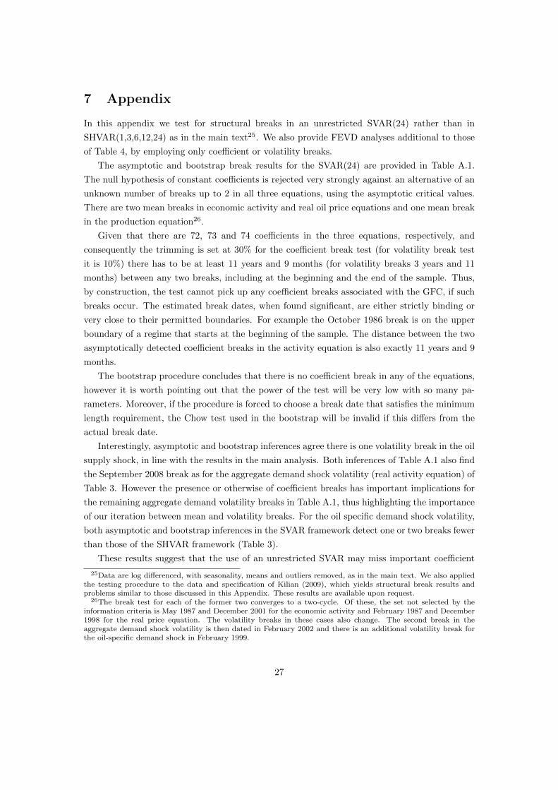
7 Appendix

In this appendix we test for structural breaks in an unrestricted SVAR(24) rather than in

SHVAR(1,3,6,12,24) as in the main text25. We also provide FEVD analyses additional to those

of Table 4, by employing only coefficient or volatility breaks.

The asymptotic and bootstrap break results for the SVAR(24) are provided in Table A.1.

The null hypothesis of constant coefficients is rejected very strongly against an alternative of an

unknown number of breaks up to 2 in all three equations, using the asymptotic critical values.

There are two mean breaks in economic activity and real oil price equations and one mean break

in the production equation26.

Given that there are 72, 73 and 74 coefficients in the three equations, respectively, and

consequently the trimming is set at 30% for the coefficient break test (for volatility break test

it is 10%) there has to be at least 11 years and 9 months (for volatility breaks 3 years and 11

months) between any two breaks, including at the beginning and the end of the sample. Thus,

by construction, the test cannot pick up any coefficient breaks associated with the GFC, if such

breaks occur. The estimated break dates, when found significant, are either strictly binding or

very close to their permitted boundaries. For example the October 1986 break is on the upper

boundary of a regime that starts at the beginning of the sample. The distance between the two

asymptotically detected coefficient breaks in the activity equation is also exactly 11 years and 9

months.

The bootstrap procedure concludes that there is no coefficient break in any of the equations,

however it is worth pointing out that the power of the test will be very low with so many pa-

rameters. Moreover, if the procedure is forced to choose a break date that satisfies the minimum

length requirement, the Chow test used in the bootstrap will be invalid if this differs from the

actual break date.

Interestingly, asymptotic and bootstrap inferences agree there is one volatility break in the oil

supply shock, in line with the results in the main analysis. Both inferences of Table A.1 also find

the September 2008 break as for the aggregate demand shock volatility (real activity equation) of

Table 3. However the presence or otherwise of coefficient breaks has important implications for

the remaining aggregate demand volatility breaks in Table A.1, thus highlighting the importance

of our iteration between mean and volatility breaks. For the oil specific demand shock volatility,

both asymptotic and bootstrap inferences in the SVAR framework detect one or two breaks fewer

than those of the SHVAR framework (Table 3).

These results suggest that the use of an unrestricted SVAR may miss important coefficient

25Data are log differenced, with seasonality, means and outliers removed, as in the main text. We also appliedthe testing procedure to the data and specification of Kilian (2009), which yields structural break results andproblems similar to those discussed in this Appendix. These results are available upon request.

26The break test for each of the former two converges to a two-cycle. Of these, the set not selected by theinformation criteria is May 1987 and December 2001 for the economic activity and February 1987 and December1998 for the real price equation. The volatility breaks in these cases also change. The second break in theaggregate demand shock volatility is then dated in February 2002 and there is an additional volatility break forthe oil-specific demand shock in February 1999.

27

breaks because their timing does not satisfy the minimum length requirement needed to justify

the formal statistical tests. It may also be the case that bootstrap rejects breaks detected

by the use of asymptotic critical values due to power issues and because the actual breaks

dates differ from estimated ones which satisfy the minimum length requirement. Our main

paper therefore proposes a more parsimonious specification in order to mitigate the number of

coefficients employed.

28

Tab

le1.

Un

itro

ot

test

resu

lts

wit

hst

ructu

ral

bre

aks

Oil

Pro

du

ctio

nE

con

om

icA

ctiv

ity

Rea

lO

ilP

rice

Pan

ela:

Tes

tsfo

rst

ruct

ura

lb

reaks

intr

end

Sta

tist

ic5%

Cri

t.va

l.S

tati

stic

5%

Cri

t.va

l.S

tati

stic

5%

Cri

t.va

l.0

v1

bre

ak11

.58*

3.1

68.9

2*

3.1

68.1

8*

3.1

61

v2

bre

ak10

.17*

3.6

62.7

93.6

616.8

7*

3.6

62

v3

bre

aks

7.32*

3.7

110.5

0*

3.7

13

v4

bre

aks

7.82*

3.9

626.5

7*

3.9

64

v5

bre

aks

245.9

3*

4.1

326.5

7*

4.1

3P

anel

b:

GL

S-d

etre

nd

edu

nit

root

test

sall

owin

gtr

end

bre

aks

Sta

tist

ic5%

Cri

t.va

l.S

tati

stic

5%

Cri

t.va

l.S

tati

stic

5%

Cri

t.va

l.N

ob

reak

5.7

75.5

44.7

7*

5.5

415.5

65.5

41

bre

ak9.2

66.3

94.5

6*

4.8

718.0

47.4

02

bre

aks

10.4

56.4

96.8

4*

6.9

021.8

07.1

23

bre

aks

8.5

57.6

19.1

67.1

45.0

3*

7.1

14

bre

aks

12.1

38.7

79.1

88.2

97.5

0*

8.4

05

bre

aks

7.1

2*

9.5

18.7

88.5

111.9

38.4

9

Not

es:

Th

ete

stin

the

firs

tro

wof

pan

ela

isth

eex

pon

enti

al

Wald

stati

stic

dis

cuss

edby

Per

ron

an

dY

ab

u(2

009)

for

on

eb

reak

inb

oth

slop

ean

dle

vel,

vali

dfo

rb

oth

I(0)

and

I(1)

erro

rco

mp

on

ents

,w

hil

eth

ose

inth

ere

main

ing

row

sare

the

sup

rem

aof

that

stati

stic

wh

enap

pli

edto

the

sub

sam

ple

sd

efin

edu

nder

the

corr

esp

on

din

gnull

,th

ecr

itic

al

valu

esfo

rsu

chse

qu

enti

all

yap

pli

edst

ati

stic

sb

ein

gp

rovid

edin

Kej

riw

alan

dP

erro

n(2

010)

.S

tati

stic

sin

pan

elb

are

GL

S-d

etre

nd

edM

un

itro

ot

test

stati

stic

s,an

aly

sed

by

Ng

an

dP

erro

n(2

001)

for

no

tren

db

reak

san

dex

tend

edby

Car

rion

-i-S

ilve

stre

etal.

(2009)

tom

ult

iple

bre

aks;

bold

stati

stic

sco

rres

pon

dto

the

num

ber

of

bre

aks

sele

cted

thro

ugh

the

Kej

riw

alan

dP

erro

n(2

010)

pro

ced

ure

.*In

dic

ate

sth

ere

ject

ion

of

the

rele

vant

null

hyp

oth

esis

(nam

ely,

the

low

ernu

mb

erof

ind

icat

edb

reak

sin

pan

ela

and

pre

sen

ceof

au

nit

root

inp

an

elb

)at

the

5%

level

.R

ejec

tion

inp

an

ela

(pan

elb

)ap

pli

esw

hen

the

stat

isti

cis

grea

ter

(les

s)th

anth

ecr

itic

al

valu

e.A

llcr

itic

al

valu

esare

asy

mp

toti

can

dfr

om

the

ind

icate

dst

ud

ies.

29

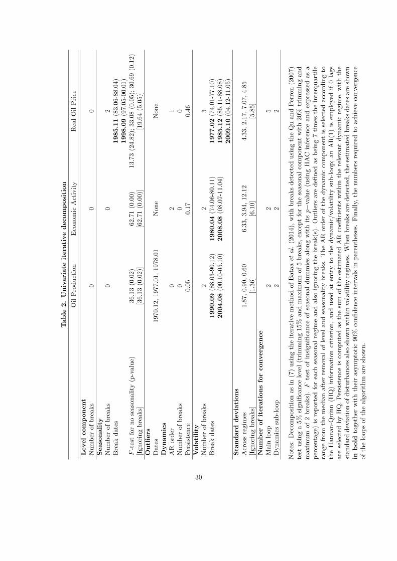
Tab

le2.

Un

ivari

ate

itera

tive

decom

posi

tion

Oil

Pro

du

ctio

nE

con

om

icA

ctiv

ity

Rea

lO

ilP

rice

Level

com

pon

ent

Nu

mb

erof

bre

aks

00

0S

easo

nali

tyN

um

ber

ofb

reak

s0

02

Bre

akd

ates

1985.1

1(8

3.0

6-8

8.0

4)

1998.0

9(9

7.0

5-0

0.0

1)

F-t

est

for

no

seas

onal

ity

(p-v

alu

e)36.1

3(0

.02)

62.7

1(0

.00)

13.7

3(2

4.8

2);

33.0

8(0

.05);

30.6

9(0

.12)

[Ign

orin

gb

reak

s][3

6.1

3(0

.02)]

[62.7

1(0

.00)]

[19.6

4(5

.05)]

Ou

tlie

rsD

ates

1970.1

2,

1977.0

1,

1978.0

1N

on

eN

on

eD

yn

am

ics

AR

ord

er0

21

Nu

mb

erof

bre

aks

00

0P

ersi

sten

ce0.0

50.1

70.4

6V

ola

tili

tyN

um

ber

ofb

reak

s2

23

Bre

akd

ates

1990.0

9(8

8.0

3-9

0.1

2)

1980.0

4(7

4.0

6-8

0.1

1)

1977.0

2(7

4.0

1-7

7.1

0)

2004.0

8(0

0.1

0-0

5.1

0)

2008.0

8(0

8.0

7-1

1.0

4)

1985.1

2(8

5.1

1-8

8.0

8)

2009.1

0(0

4.1

2-1

1.0

5)

Sta

nd

ard

devia

tion

sA

cros

sre

gim

es1.8

7,

0.9

0,

0.6

06.3

3,

3.9

4,

12.1

24.3

3,

2.1

7,7.0

7,

4.8

5[I

gnor

ing

bre

aks]

[1.3

6]

[6.1

0]

[5.8

5]

Nu

mb

er

of

itera

tion

sfo

rconverg

en

ce

Mai

nlo

op2

25

Dyn

amic

ssu

b-l

oop

22

2

Not

es:

Dec

omp

osit

ion

asin

(7)

usi

ng

the

iter

ati

vem

eth

od

of

Bata

aet

al.

(2014),

wit

hb

reaks

det

ecte

du

sin

gth

eQ

uan

dP

erro

n(2

007)

test

usi

ng

a5%

sign

ifica

nce

level

(tri

mm

ing

15%

an

dm

axim

um

of

5b

reaks,

exce

pt

for

the

seaso

nal

com

pon

ent

wit

h20%

trim

min

gan

dm

axim

um

of2

bre

aks)

.F

test

ofin

sign

ifica

nce

of

seaso

nal

du

mm

ies

alo

ng

wit

hit

sp−

valu

e(u

sin

gH

AC

infe

ren

cean

dex

pre

ssed

as

ap

erce

nta

ge)

isre

por

ted

for

each

seas

onal

regim

ean

dals

oig

nori

ng

the

bre

ak(s

).O

utl

iers

are

defi

ned

as

bei

ng

7ti

mes

the

inte

rqu

art

ile

ran

gefr

omth

em

edia

naf

ter

rem

oval

ofle

vel

an

dse

aso

nali

tyb

reaks.

Th

eA

Rord

erof

the

dyn

am

icco

mp

on

ent

isse

lect

edacc

ord

ing

toth

eH

ann

an-Q

uin

n(H

Q)

info

rmat

ion

crit

erio

n,

an

du

sed

at

entr

yto

the

dyn

am

ic/vola

tility

sub

-loop

;an

AR

(1)

isem

plo

yed

if0

lags

are

sele

cted

by

HQ

.P

ersi

sten

ceis

com

pu

ted

as

the

sum

of

the

esti

mate

dA

Rco

effici

ents

wit

hin

the

rele

vant

dyn

am

icre

gim

e,w

ith

the

stan

dar

dd

evia

tion

ofd

istu

rban

ces

also

show

nw

ith

invo

lati

lity

regim

es.

Wh

enb

reaks

are

det

ecte

d,

the

esti

mate

db

reaks

date

sare

show

nin

bold

toge

ther

wit

hth

eir

asym

pto

tic

90%

con

fid

ence

inte

rvals

inp

are

nth

eses

.F

inall

y,th

enum

ber

sre

qu

ired

toach

ieve

conve

rgen

ceof

the

loop

sof

the

algo

rith

mar

esh

own

.

30

Table 3. Coefficient and variance break test results for the oil market SHVAR

Oil Production Economic Activity Real Oil Price

I (A). Coefficients breaksOverall test 255.42* (38.82) 206.82* (40.86) 243.78* (42.61)

Seq(2/1) 33.26 (37.63) 36.71 (39.37) 51.29* (41.22)Seq(3/2) 57.51* (42.59)Seq(4/3) 57.51* (43.89)

bootstrap p-value 0.1 24.47 85.42for each break 83.34

1.081.42

Break 1 1980.12 1988.05(80.10-81.02) (88.02-88.08)

Break 2 1994.10(94.07-95.01)

I (B). Contemporaneous coefficients

n.a. a21 a31 a32Across regimes - -0.17 0.06, -1.81, -0.42 0.17, 0.03, 0.20

[Ignoring breaks] - [-0.17] [-0.28] [0.16]

II (A). Variance breaksOverall test 137.75* 171.81* 126.69*

Seq(2/1) 17.11* 24.06* 21.79*Seq(3/2) 9.89 5.34 21.63*Seq(4/3) 12.14

bootstrap p-value 0.0 0.04 0.40for each break 0.31 0.0 0.0

0.15Break 1 1990.10 1979.09 1981.03

(88.02-91.01) (73.04-80.02) (79.06-81.11)Break 2 2004.09 2008.09 1986.02

(99.08-06.04) (08.08-11.06) (86.01-86.12)Break 3 1998.09

(98.01-09.11)

II (B). Shock standard deviations

σoils σaggd σoildAcross regimes 1.67, 0.86, 0.60 6.21, 3.94, 11.88 2.65, 1.60, 4.64, 6.72

[Ignoring breaks] [1.31] [5.98] [5.61]

III. Number of iterations required to converge

3 2 4

IV. F statistic (bootstrap p-value) for SHVAR restrictionsRegime I n.c. 1.28 (15.2) 1.08 (24.6)Regime II 0.92 (70.9) - n.c.Regime III - - 1.56 (12.8)All sample 0.94 (72.3) 1.28 (36.3) 1.42 (30.47)

Notes: Values reported in panels I (A) and II (A) are at convergence of the iterative procedure of Bataa, Osborn,Sensier and van Dijk (2013). The overall test examines the null hypothesis of no break against an unknownnumber of breaks, to a maximum of 5 breaks for each SHVAR equation and 8 for the variance. If the overallstatistic is significant at 5%, sequential tests are applied starting with the null hypothesis of one break andcontinuing until the relevant statistic is not significant. Asymptotic critical values for the 5% significance levelare reported next to respective test statistics in parenthesis in panel II (A) since the number of parameters aredifferent in the SVAR equations. The critical values for shock volatilities applicable to II (B) are 10.67, 10.97,11.88 and 12.49 for the Overall test, Seq(2/1), Seq(3/2), and Seq(4/3), respectively. * indicates the statisticis significant at 5%. The estimated break dates and their 90% confidence intervals (in parenthesis) are alsoreported. Bootstrap p-values corresponding to the null hypothesis that an asymptotically detected break doesnot exist are also reported. Panels I (B) and II (B) show estimated contemporaneous coefficients and shockstandard deviations respectively across sub-samples defined by the break dates. Also shown in square bracketsare those quantities that ignore the breaks. Panel III reports the number of iterations required to convergein coefficient and volatility break dates. The last panel reports on the validity of the SHVAR restrictions byF tests over the sub-samples defined by the mean break dates and over the whole sample. The asymptotic5% critical value from F (60,∞) is 1.32. n.c. indicates it was impossible to compute the F statistic over thesub-sample due to non-invertability issue (too many parameters with not long enough sub-sample).

31

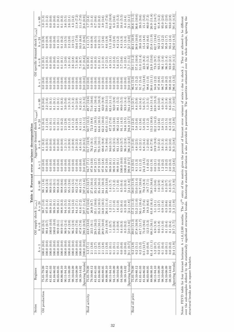
Tab

le4.

Forecast

error

varia

nce

decom

posi

tion

Ser

ies

Reg

imes

Oil

sup

ply

shock

(εoils)

Aggre

gate

dem

an

dsh

ock

(εaggd)

Oil

spec

ific

dem

an

dsh

ock

(εoild)

h=

1h

=6

h=

24

h=

60

h=

1h

=6

h=

24

h=

60

h=

1h

=6

h=

24

h=

60

Oil

pro

du

ctio

n75.0

1-7

9.0

9100.0

(0.0

)99.6

(0.5

)98.7

(1.0

)98.1

(1.6

)0.0

(0.0

)0.1

(0.2

)0.5

(0.4

)0.9

(0.6

)0.0

(0.0

)0.3

(0.5

)0.9

(0.9

)1.0

(1.3

)79.1

0-8

0.1

2100.0

(0.0

)99.4

(0.7

)97.9

(1.4

)96.8

(2.3

)0.0

(0.0

)0.3

(0.5

)1.2

(1.0

)2.2

(1.6

)0.0

(0.0

)0.3

(0.5

)0.9

(0.9

)1.0

(1.2

)81.0

1-8

1.0

3100.0

(0.0

)100.0

(0.0

)99.9

(0.1

)99.9

(0.1

)0.0

(0.0

)0.0

(0.0

)0.1

(0.1

)0.1

(0.1

)0.0

(0.0

)0.0

(0.0

)0.0

(0.0

)0.0

(0.0

)81.0

4-8

6.0

2100.0

(0.0

)100.0

(0.0

)99.9

(0.1

)99.9

(0.1

)0.0

(0.0

)0.0

(0.0

)0.1

(0.1

)0.1

(0.1

)0.0

(0.0

)0.0

(0.0

)0.0

(0.0

)0.0

(0.0

)86.0

3-8

8.0

5100.0

(0.0

)99.9

(0.1

)99.8

(0.1

)99.8

(0.2

)0.0

(0.0

)0.0

(0.0

)0.1

(0.1

)0.1

(0.1

)0.0

(0.0

)0.1

(0.1

)0.1

(0.1

)0.1

(0.2

)88.0

6-9

0.1

0100.0

(0.0

)99.9

(0.1

)99.8

(0.3

)99.8

(0.6

)0.0

(0.0

)0.0

(0.0

)0.1

(0.2

)0.1

(0.3

)0.0

(0.0

)0.1

(0.1

)0.1

(0.2

)0.1

(0.3

)90.1

1-9

4.1

0100.0

(0.0

)96.9

(2.4

)94.4

(5.5

)93.5

(9.0

)0.0

(0.0

)1.2

(1.1

)2.5

(2.9

)3.0

(5.0

)0.0

(0.0

)1.9

(2.0

)3.0

(3.5

)3.6

(5.5

)94.1

1-9

8.0

9100.0

(0.0

)97.4

(2.0

)95.9

(2.4

)95.5

(2.6

)0.0

(0.0

)1.0

(0.9

)1.8

(1.2

)1.9

(1.3

)0.0

(0.0

)1.6

(1.8

)2.3

(2.0

)2.6

(2.1

)98.1

0-0

4.0

9100.0

(0.0

)96.3

(2.9

)94.3

(3.3

)93.8

(3.5

)0.0

(0.0

)1.0

(0.9

)1.8

(1.2

)1.8

(1.2

)0.0

(0.0

)2.6

(2.8

)3.9

(3.1

)4.3

(3.2

)04.1

0-0

8.0

9100.0

(0.0

)89.6

(7.0

)84.4

(7.1

)83.2

(7.4

)0.0

(0.0

)2.9

(2.3

)4.9

(2.9

)5.0

(2.9

)0.0

(0.0

)7.5

(6.9

)10.6

(7.0

)11.8

(7.2

)08.1

0-1

4.0

2100.0

(0.0

)87.8

(7.0

)81.6

(7.2

)80.4

(7.5

)0.0

(0.0

)4.8

(3.4

)8.1

(4.1

)8.2

(4.1

)0.0

(0.0

)7.4

(6.7

)10.3

(6.8

)11.4

(7.0

)[I

gn

ori

ng

bre

aks]

[100.0

(0.0

)][9

9.2

(0.9

)][9

7.7

(1.4

)][9

7.3

(1.6

)][0

.0(0

.0)]

[0.2

(0.5

)][1

.6(1

.1)]

[1.8

(1.3

)][0

.0(0

.0)]

[0.7

(0.8

)][0

.7(0

.9)]

[0.8

(0.9

)]R

eal

act

ivit

y75.0

1-7

9.0

95.3

(7.1

)43.8

(13.0

)47.9

(12.6

)48.5

(12.7

)94.7

(7.1

)55.7

(12.9

)50.7

(12.5

)49.7

(12.6

)0.0

(0.0

)0.6

(0.8

)1.4

(1.7

)1.7

(2.4

)79.1

0-8

0.1

22.1

(3.0

)23.5

(9.1

)26.9

(9.7

)27.4

(10.4

)97.9

(3.0

)76.2

(9.1

)72.3

(9.8

)71.6

(10.6

)0.0

(0.0

)0.3

(0.4

)0.8

(0.9

)1.0

(1.4

)81.0

1-8

1.0

32.1

(2.7

)29.5

(10.2

)35.1

(10.6

)35.2

(10.5

)97.9

(2.7

)70.1

(10.1

)64.3

(10.5

)64.1

(10.4

)0.0

(0.0

)0.4

(0.3

)0.6

(0.5

)0.7

(0.6

)81.0

4-8

6.0

22.1

(2.9

)29.6

(10.1

)35.3

(10.5

)35.4

(10.4

)97.9

(2.9

)70.3

(10.1

)64.6

(10.5

)64.4

(10.3

)0.0

(0.0

)0.1

(0.1

)0.2

(0.1

)0.2

(0.2

)86.0

3-8

8.0

52.1

(2.8

)28.9

(10.0

)34.0

(10.5

)34.1

(10.3

)97.9

(2.8

)68.6

(9.8

)62.3

(10.0

)62.0

(9.9

)0.0

(0.0

)2.4

(1.9

)3.7

(2.6

)3.9

(3.6

)88.0

6-9

0.1

02.1

(3.0

)24.4

(9.9

)26.4

(11.4

)29.4

(13.0

)97.9

(3.0

)71.8

(9.6

)65.0

(11.3

)59.0

(13.1

)0.0

(0.0

)3.7

(2.5

)8.6

(4.9

)11.6

(7.6

)90.1

1-9

4.1

00.1

(0.1

)1.1

(0.7

)1.2

(1.1

)1.4

(1.7

)99.9

(0.1

)94.0

(3.1

)87.2

(7.0

)82.4

(11.1

)0.0

(0.0

)4.9

(3.1

)11.5

(6.8

)16.2

(10.8

)94.1

1-9

8.0

90.1

(0.1

)1.3

(0.8

)1.7

(1.0

)1.7

(1.2

)99.9

(0.1

)95.3

(2.5

)93.3

(3.0

)92.0

(3.9

)0.0

(0.0

)3.4

(2.3

)5.0

(2.8

)6.3

(3.6

)98.1

0-0

4.0

90.1

(0.1

)1.3

(0.8

)1.6

(1.0

)1.7

(1.0

)99.9

(0.1

)93.1

(3.8

)90.2

(4.4

)88.1

(5.5

)0.0

(0.0

)5.6

(3.7

)8.2

(4.2

)10.3

(5.3

)04.1

0-0

8.0

90.0

(0.0

)0.4

(0.3

)0.5

(0.4

)0.5

(0.4

)100.0

(0.0

)93.9

(3.7

)91.1

(4.3

)89.0

(5.5

)0.0

(0.0

)5.7

(3.6

)8.3

(4.3

)10.4

(5.5

)08.1

0-1

4.0

20.0

(0.0

)0.3

(0.2

)0.3

(0.3

)0.3

(0.3

)100.0

(0.0

)96.3

(2.8

)94.6

(3.5

)93.3

(4.4

)0.0

(0.0

)3.4

(2.8

)5.1

(3.4

)6.4

(4.4

)[I

gn

ori

ng

bre

aks]

[0.1

(0.7

)][2

.0(1

.6)]

[2.4

(1.8

)][2

.4(1

.8)]

[99.9

(0.7

)][9

6.3

(2.3

)][9

4.8

(2.7

)][9

4.4

(2.9

)][0

.0(0

.0)]

[1.7

(1.5

)][2

.7(2

.0)]

[3.1

(2.1

)]R

eal

oil

pri

ce75.0

1-7

9.0

90.2

(4.9

)39.0

(11.3

)57.3

(11.3

)58.0

(11.9

)3.3

(0.5

)1.9

(1.0

)2.4

(2.2

)3.5

(2.7

)96.5

(5.0

)59.1

(11.2

)40.4

(10.9

)38.6

(11.5

)79.1

0-8

0.1

20.2

(5.1

)37.8

(10.9

)55.2

(11.0

)55.0

(11.4

)8.1

(1.3

)4.8

(2.5

)5.8

(5.0

)8.4

(5.9

)91.7

(5.2

)57.4

(10.8

)38.9

(10.0

)36.6

(10.6

)81.0

1-8

1.0

30.2

(5.2

)44.7

(11.7

)56.1

(10.4

)56.7

(10.8

)8.1

(1.2

)4.3

(2.1

)4.1

(3.8

)4.0

(4.4

)91.7

(5.4

)51.0

(11.4

)39.8

(9.3

)39.3

(9.6

)81.0

4-8

6.0

20.5

(12.7

)71.0

(9.6

)78.8

(7.6

)79.3

(8.3

)24.2

(3.5

)6.8

(3.4

)5.8

(5.0

)5.6

(5.7

)75.3

(12.8

)22.3

(8.3

)15.4

(4.8

)15.1

(5.0

)86.0

3-8

8.0

50.0

(0.9

)12.3

(5.3

)18.3

(6.6

)18.7

(7.1

)1.4

(0.2

)1.2

(0.6

)1.4

(1.2

)1.3

(1.5

)98.6

(1.0

)86.5

(5.3

)80.3

(6.6

)80.0

(7.3

)88.0

6-9

0.1

061.4

(11.1

)68.3

(16.1

)61.0

(16.4

)58.3

(16.6

)0.0

(1.9

)6.8

(7.9

)13.2

(10.8

)14.8

(11.4

)38.6

(11.1

)24.9

(13.6

)25.8

(11.9

)26.9

(11.8

)90.1

1-9

4.1

05.2

(0.7

)6.9

(1.9

)5.1

(3.1

)4.6

(3.6

)0.0

(2.1

)19.9

(9.8

)32.2

(14.2

)33.9

(15.3

)94.8

(2.2

)73.3

(9.7

)62.7

(13.6

)61.6

(14.7

)94.1

1-9

8.0

90.2

(0.7

)0.6

(1.8

)1.5

(2.7

)1.6

(2.9

)2.0

(0.4

)5.9

(2.3

)6.2

(2.6

)6.6

(3.0

)97.8

(0.8

)93.5

(2.9

)92.3

(3.7

)91.8

(4.2

)98.1

0-0

4.0

90.1

(0.4

)0.4

(1.0

)0.9

(1.6

)1.0

(1.8

)1.2

(0.2

)3.6

(1.3

)3.8

(1.5

)4.0

(1.8

)98.7

(0.5

)96.1

(1.6

)95.3

(2.2

)95.0

(2.6

)04.1

0-0

8.0

90.0

(0.1

)0.1

(0.4

)0.3

(0.6

)0.3

(0.7

)1.2

(0.2

)3.6

(1.3

)3.8

(1.5

)4.0

(1.8

)98.8

(0.2

)96.3

(1.4

)95.9

(1.7

)95.7

(2.0

)08.1

0-1

4.0

20.0

(0.2

)0.1

(0.4

)0.3

(0.6

)0.3

(0.7

)2.0

(0.3

)6.0

(2.0

)6.3

(2.3

)6.6

(2.8

)98.0

(0.4

)93.9

(2.1

)93.4

(2.4

)93.0

(2.9

)[I

gn

ori

ng

bre

aks]

[0.4

(1.9

)][0

.7(1

.7)]

[1.3

(1.9

)][1

.3(1

.9)]

[3.0

(2.6

)][6

.3(3

.8)]

[6.7

(3.9

)][7

.1(4

.0)]

[96.6

(3.3

)][9

3.0

(4.1

)][9

2.0

(4.3

)][9

1.6

(4.3

)]

Note

s:F

EV

Dta

ble

for

fou

rfo

reca

sthori

zon

s:h

=1,6

,12,6

0m

onth

s.T

heij

then

try

of

the

matr

ixgiv

esth

ep

erce

nt

of

fore

cast

erro

rvari

an

ceof

seri

esi

du

eto

shock

j.T

hey

are

allow

edto

be

diff

eren

tover

the

sub

-sam

ple

sd

efin

edby

the

stati

stic

ally

sign

ifica

nt

stru

ctu

ral

bre

aks.

Boots

trap

stan

dard

dev

iati

on

isals

op

rovid

edin

pare

nth

esis

.T

he

qu

anti

ties

esti

mate

dover

the

wh

ole

sam

ple

,ig

nori

ng

the

stru

ctu

ral

bre

aks

are

insq

uare

bra

cket

s.

32

Tab

leA

.1.

Coeffi

cie

nt

an

dvaria

nce

break

test

resu

lts

for

the

oil

market

SV

AR

Asy

mp

toti

cin

fere

nce

Boots

trap

infe

ren

ce

Oil

Pro

du

ctio

nE

con

om

icA

ctiv

ity

Rea

lO

ilP

rice

Oil

Pro

du

ctio

nE

con

om

icA

ctiv

ity

Rea

lO

ilP

rice

I(A

).C

oeffi

cien

tsbr

eaks

Over

all

test

238.2

9*

[113.3

6]

187.4

8*

[114.8

9]

208.5

6*

[116.3

5]

245.8

1*

[113.3

6]

176.9

6*

[114.8

9]

226.6

3*

[116.3

5]

Seq

(2/1)

97.4

1[1

13.9

0]

115.8

1*

[114.2

0]

150.7

4*

[116.5

9]

99.1

7[1

13.9

0]

114.5

0*

[114.2

0]

131.7

1*

[116.5

9]

boots

trapp-v

alu

en

.a.

n.a

.n

.a.

15.6

599.0

319.5

9fo

rea

chb

reak

n.a

.n

.a.

n.a

.67.9

228.8

3B

reak

11986.1

01987.0

21987.1

0[8

6.0

9-8

6.1

1]

[86.1

1-8

7.0

5]

[87.0

8-8

7.1

2]

Bre

ak

21998.1

12001.0

7[9

8.0

8-9

9.0

2]

[01.0

5-0

1.0

9]

I(B

).C

on

tem

pora

neo

us

coeffi

cien

ts

n.a

.a21

a31

a32

n.a

.a21

a31

a32

Acr

oss

regim

es-

-0.1

24,

-0.4

49,

0.4

60

0.0

03,

-0.9

21,

-0.8

08

0.2

14,

0.1

31,

0.2

17

--0

.104

-0.2

46

0.2

02

[Ign

ori

ng

bre

aks]

-[-

0.1

04]

[-0.2

67]

[0.2

02]

-[-

0.1

04]

[-0.2

67]

[0.2

02]

II(A

).V

ari

an

cebr

eaks

Over

all

test

80.5

4*

[10.6

7]

140.5

2*

[10.6

7]

94.4

7*

[10.6

7]

120.6

5*

[10.6

7]

141.9

6[1

0.6

7]

85.1

7*

[10.6

7]

Seq

(2/1)

7.6

3[1

0.9

7]

23.3

6*

[10.9

7]

8.6

3[1

0.9

7]

9.1

9[1

0.9

7]

17.4

7*

[10.9

7]

17.0

0*

[10.9

7]

Seq

(3/2)

20.9

6*

[11.8

8]

6.1

3[1

1.8

8]

3.8

8[1

1.8

8]

7.4

2[1

1.8

8]

Seq

(4/3)

9.8

1[1

2.4

9]

boots

trapp-v

alu

en

.a.

n.a

.n

.a.

0.0

0.0

20.3

1fo

rea

chb

reak

n.a

.n

.a.

n.a

.0.0

0.0

Bre

ak

11990.1

01986.0

31986.0

21990.1

01980.0

51981.0

3[8

7.0

7-9

1.0

3]

[82.0

2-8

7.0

3]

[86.0

1-8

9.0

6]

[88.0

8-9

1.0

1]

73.0

4-8

0.1

2[7

8.0

8-8

1.1

0]

Bre

ak

21998.1

22008.0

91985.1

2[9

8.0

7-0

1.0

2]

[08.0

8-1

1.0

2]

[85.1

1-8

7.0

3]

Bre

ak

32008.0

9[0

8.0

6-1

2.0

5]

II(B

).S

hoc

kst

an

da

rdd

evia

tio

ns

σ2 oils

σ2 aggd

σ2 oild

σ2 oils

σ2 aggd

σ2 oild

Acr

oss

regim

es1.5

90,

0.4

87

12.7

3,

5.9

0,

19.6

5,

77.1

53.8

8,

19.6

32.7

44,

0.6

40

31.2

7,

17.7

1,

110.8

49.8

8,

3.7

9,

34.1

9[I

gn

ori

ng

bre

aks]

[1.4

8]

[30.3

0]

[26.6

9]

[1.4

8]

[30.3

0]

[26.6

9]

III.

Nu

mbe

ro

fit

era

tio

ns

requ

ired

toco

nve

rge

319

19

22

2

Not

es:

See

Not

esto

Tab

le3

inth

em

ain

text.

n.c

.m

ean

sth

edate

was

som

em

onth

souts

ide

the

sam

ple

per

iod

,th

us

not

calc

ula

ted

.n

.a.

mea

ns

not

ap

pli

catb

le.

33

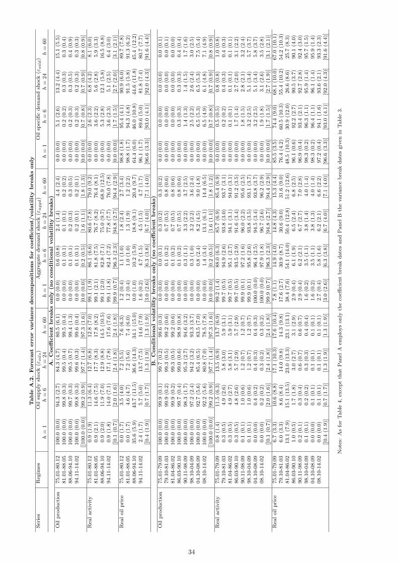
Tab

leA

.2.

Forecast

error

varia

nce

decom

posi

tion

sfo

rcoeffi

cie

nt/

vola

tili

tyb

reaks

on

lyS

erie

sR

egim

esO

ilsu

pp

lysh

ock

(εoils)

Aggre

gate

dem

an

dsh

ock

(εaggd)

Oil

spec

ific

dem

an

dsh

ock

(εoild)

h=

1h

=6

h=

24

h=

60

h=

1h

=6

h=

24

h=

60

h=

1h

=6

h=

24

h=

60

A.

Coeffi

cie

nt

breaks

on

ly(n

ocon

dit

ion

al

vola

tili

tyb

reaks)

Oil

pro

du

ctio

n75.0

1-8

0.1

2100.0

(0.0

)94.3

(2.7

)84.3

(4.7

)80.5

(6.1

)0.0

(0.0

)0.6

(0.8

)2.4

(1.4

)4.4

(2.4

)0.0

(0.0

)5.1

(2.6

)13.2

(4.4

)15.1

(5.5

)81.0

1-8

8.0

5100.0

(0.0

)99.8

(0.3

)99.5

(0.4

)99.5

(0.4

)0.0

(0.0

)0.1

(0.1

)0.1

(0.1

)0.2

(0.2

)0.0

(0.0

)0.2

(0.2

)0.3

(0.3

)0.3

(0.4

)88.0

6-9

4.1

0100.0

(0.0

)99.7

(0.3

)99.5

(0.7

)99.4

(1.3

)0.0

(0.0

)0.1

(0.1

)0.2

(0.3

)0.3

(0.5

)0.0

(0.0

)0.2

(0.3

)0.3

(0.5

)0.4

(0.9

)94.1

1-1

4.0

2100.0

(0.0

)99.8

(0.3

)99.6

(0.3

)99.6

(0.4

)0.0

(0.0

)0.1

(0.1

)0.2

(0.1

)0.2

(0.1

)0.0

(0.0

)0.2

(0.3

)0.2

(0.3

)0.3

(0.3

)[[100.0

(0.0

)][9

9.2

(0.9

)][9

7.7

(1.4

)][9

7.3

(1.6

)][0

.0(0

.0)]

[0.2

(0.5

)][1

.6(1

.1)]

[1.8

(1.3

)][0

.0(0

.0)]

[0.7

(0.8

)][0

.7(0

.9)]

[0.8

(0.9

)]R

eal

act

ivit

y75.0

1-8

0.1

20.9

(1.9

)11.3

(6.4

)12.7

(6.8

)12.8

(7.0

)99.1

(1.9

)86.1

(6.6

)80.6

(7.8

)79.0

(9.2

)0.0

(0.0

)2.6

(2.3

)6.8

(4.2

)8.1

(6.0

)81.0

1-8

8.0

50.9

(2.1

)14.6

(7.5

)17.7

(8.3

)17.8

(8.2

)99.1

(2.1

)81.8

(7.5

)76.7

(8.2

)76.4

(8.1

)0.0

(0.0

)3.6

(2.2

)5.6

(2.8

)5.9

(3.3

)88.0

6-9

4.1

00.9

(2.0

)11.9

(7.0

)12.9

(8.8

)14.5

(10.5

)99.1

(2.0

)82.8

(7.1

)75.0

(9.7

)68.9

(12.5

)0.0

(0.0

)5.3

(2.8

)12.1

(5.8

)16.5

(8.8

)94.1

1-1

4.0

20.9

(1.8

)14.0

(7.1

)17.1

(7.8

)17.6

(7.6

)99.1

(1.8

)82.4

(7.2

)77.8

(7.7

)76.0

(7.8

)0.0

(0.0

)3.6

(2.3

)5.1

(2.5

)6.4

(3.0

)[[0.1

(0.7

)][2

.0(1

.6)]

[2.4

(1.8

)][2

.4(1

.8)]

[99.9

(0.7

)][9

6.3

(2.3

)][9

4.8

(2.7

)][9

4.4

(2.9

)][0

.0(0

.0)]

[1.7

(1.5

)][2

.7(2

.0)]

[3.1

(2.1

)]R

eal

oil

pri

ce75.0

1-8

0.1

20.0

(1.7

)3.5

(4.0

)7.2

(5.5

)7.6

(6.3

)1.2

(0.4

)1.1

(1.0

)1.8

(2.4

)2.7

(3.4

)98.8

(1.8

)95.4

(4.1

)90.9

(6.0

)89.7

(7.8

)81.0

1-8

8.0

50.0

(1.7

)4.6

(4.7

)7.2

(5.6

)7.4

(6.0

)1.2

(0.4

)1.0

(1.0

)1.3

(1.9

)1.2

(2.2

)98.8

(1.7

)94.3

(4.8

)91.5

(5.8

)91.3

(6.2

)88.0

6-9

4.1

035.6

(5.9

)43.7

(11.5

)36.6

(14.3

)34.1

(15.0

)0.0

(1.0

)10.2

(5.9

)18.8

(9.1

)20.4

(9.7

)64.4

(6.0

)46.0

(10.8

)44.6

(11.8

)45.4

(12.2

)94.1

1-1

4.0

22.4

(1.7

)5.7

(5.0

)13.7

(7.5

)14.6

(7.9

)1.6

(0.2

)4.7

(1.5

)4.5

(1.5

)4.7

(1.7

)96.1

(1.7

)89.6

(5.0

)81.8

(7.4

)80.7

(7.7

)[[0.4

(1.9

)][0

.7(1

.7)]

[1.3

(1.9

)][1

.3(1

.9)]

[3.0

(2.6

)][6

.3(3

.8)]

[6.7

(4.0

)][7

.1(4

.0)]

[96.6

(3.3

)][9

3.0

(4.1

)][9

2.0

(4.3

)][9

1.6

(4.4

)]B

.C

on

dit

ion

al

vola

tili

tyb

reaks

on

ly(n

ocoeffi

cie

nt

breaks)

Oil

pro

du

ctio

n75.0

1-7

9.0

9100.0

(0.0

)99.9

(0.1

)99.7

(0.2

)99.6

(0.3

)0.0

(0.0

)0.0

(0.1

)0.3

(0.2

)0.3

(0.2

)0.0

(0.0

)0.0

(0.0

)0.0

(0.0

)0.0

(0.1

)79.1

0-8

1.0

3100.0

(0.0

)99.9

(0.2

)99.3

(0.5

)99.2

(0.6

)0.0

(0.0

)0.1

(0.2

)0.7

(0.5

)0.8

(0.6

)0.0

(0.0

)0.0

(0.0

)0.0

(0.0

)0.0

(0.1

)81.0

4-8

6.0

2100.0

(0.0

)99.9

(0.2

)99.3

(0.5

)99.2

(0.6

)0.0

(0.0

)0.1

(0.2

)0.7

(0.5

)0.8

(0.6

)0.0

(0.0

)0.0

(0.0

)0.0

(0.0

)0.0

(0.0

)86.0

3-9

0.1

0100.0

(0.0

)99.7

(0.4

)99.0

(0.6

)98.9

(0.8

)0.0

(0.0

)0.1

(0.2

)0.7

(0.5

)0.8

(0.6

)0.0

(0.0

)0.3

(0.3

)0.3

(0.3

)0.4

(0.4

)90.1

1-9

8.0

9100.0

(0.0

)98.3

(1.7

)95.3

(2.7

)94.6

(3.2

)0.0

(0.0

)0.3

(1.1

)3.3

(2.2

)3.7

(2.5

)0.0

(0.0

)1.4

(1.3

)1.4

(1.5

)1.7

(1.6

)98.1

0-0

4.0

9100.0

(0.0

)97.2

(2.4

)94.2

(3.2

)93.3

(3.7

)0.0

(0.0

)0.3

(1.0

)3.2

(2.2

)3.6

(2.4

)0.0

(0.0

)2.5

(2.2

)2.6

(2.4

)3.0

(2.5

)04.1

0-0

8.0

9100.0

(0.0

)92.7

(5.6

)85.4

(6.5

)83.5

(7.0

)0.0

(0.0

)0.8

(2.4

)8.2

(4.5

)9.0

(4.8

)0.0

(0.0

)6.5

(5.3

)6.5

(5.3

)7.5

(5.4

)08.1

0-1

4.0

2100.0

(0.0

)92.2

(5.6

)80.8

(7.0

)78.5

(7.8

)0.0

(0.0

)1.4

(3.4

)13.1

(6.1

)14.4

(6.5

)0.0

(0.0

)6.5

(4.9

)6.1

(4.8

)7.1

(4.9

)[[100.0

(0.0

)][9

9.2

(0.9

)][9

7.7

(1.4

)][9

7.3

(1.6

)][0

.0(0

.0)]

[0.2

(0.5

)][1

.6(1

.1)]

[1.8

(1.2

)][0

.0(0

.0)]

[0.7

(0.8

)][0

.7(0

.9)]

[0.8

(0.9

)]R

eal

act

ivit

y75.0

1-7

9.0

90.8

(1.4

)11.5

(6.3

)13.5

(6.9

)13.7

(6.9

)99.2

(1.4

)88.0

(6.3

)85.7

(6.9

)85.4

(6.9

)0.0

(0.0

)0.5

(0.5

)0.8

(0.8

)1.0

(0.8

)79.1

0-8

1.0

30.3

(0.5

)4.9

(2.6

)5.8

(3.0

)5.9

(3.1

)99.7

(0.5

)94.9

(2.6

)93.8

(3.0

)93.7

(3.1

)0.0

(0.0

)0.2

(0.2

)0.4

(0.3

)0.4

(0.3

)81.0

4-8

6.0

20.3

(0.5

)4.9

(2.7

)5.8

(3.1

)5.9

(3.1

)99.7

(0.5

)95.1

(2.7

)94.1

(3.1

)94.0

(3.1

)0.0

(0.0

)0.1

(0.1

)0.1

(0.1

)0.1

(0.1

)86.0

3-9

0.1

00.3

(0.5

)4.8

(2.6

)5.7

(2.9

)5.7

(2.9

)99.7

(0.5

)93.5

(2.9

)91.6

(3.4

)91.2

(3.5

)0.0

(0.0

)1.7

(1.4

)2.7

(2.0

)3.1

(2.2

)90.1

1-9

8.0

90.1

(0.1

)1.0

(0.6

)1.2

(0.7

)1.2

(0.7

)99.9

(0.1

)97.2

(1.6

)96.0

(2.2

)95.6

(2.5

)0.0

(0.0

)1.8

(1.5

)2.8

(2.1

)3.2

(2.4

)98.1

0-0

4.0

90.1

(0.1

)1.0

(0.6

)1.2

(0.7

)1.2

(0.7

)99.9

(0.1

)95.8

(2.6

)93.8

(3.5

)93.1

(3.7

)0.0

(0.0

)3.2

(2.5

)5.1

(3.4

)5.7

(3.7

)04.1

0-0

8.0

90.0

(0.0

)0.4

(0.2

)0.4

(0.3

)0.4

(0.3

)100.0

(0.0

)96.4

(2.5

)94.5

(3.4

)93.8

(3.7

)0.0

(0.0

)3.2

(2.5

)5.1

(3.4

)5.8

(3.7

)08.1

0-1

4.0

20.0

(0.0

)0.2

(0.2

)0.3

(0.2

)0.3

(0.2

)100.0

(0.0

)97.9

(1.8

)96.7

(2.6

)96.2

(2.9

)0.0

(0.0

)1.9

(1.8

)3.1

(2.6

)3.5

(2.8

)[[0.1

(0.7

)][2

.0(1

.6)]

[2.4

(1.8

)][2

.4(1

.8)]

[99.9

(0.7

)][9

6.3

(2.3

)][9

4.8

(2.7

)][9

4.4

(2.9

)][0

.0(0

.0)]

[1.7

(1.5

)][2

.7(1

.9)]

[3.1

(2.1

)]R

eal

oil

pri

ce75.0

1-7

9.0

96.7

(3.3

)10.6

(8.8

)17.1

(10.3

)17.6

(10.4

)7.8

(1.1

)14.9

(4.0

)14.8

(4.3

)15.3

(4.4

)85.5

(3.5

)74.4

(9.0

)68.1

(10.0

)67.0

(10.1

)79.1

0-8

1.0

36.0

(3.3

)8.6

(8.4

)14.0

(9.8

)14.3

(9.8

)17.6

(2.7

)30.9

(8.7

)30.6

(9.0

)31.6

(9.0

)76.4

(4.2

)60.5

(10.3

)55.4

(10.2

)54.2

(10.3

)81.0

4-8

6.0

213.1

(7.9

)15.1

(13.5

)23.0

(13.3

)23.1

(13.1

)38.4

(7.6

)54.1

(14.0

)50.4

(12.8

)51.2

(12.6

)48.5

(10.3

)30.9

(12.0

)26.6

(8.6

)25.7

(8.3

)86.0

3-9

0.1

01.0

(0.5

)1.7

(1.8

)3.0

(2.7

)3.1

(2.9

)2.9

(0.4

)6.1

(1.9

)6.5

(2.4

)6.8

(2.5

)96.1

(0.6

)92.2

(2.7

)90.5

(3.7

)90.1

(4.0

)90.1

1-9

8.0

90.2

(0.1

)0.3

(0.4

)0.6

(0.7

)0.6

(0.7

)2.9

(0.4

)6.2

(2.1

)6.7

(2.7

)7.0

(2.8

)96.9

(0.4

)93.4

(2.1

)92.7

(2.8

)92.4

(3.0

)98.1

0-0

4.0

90.1

(0.1

)0.2

(0.2

)0.3

(0.3

)0.4

(0.4

)1.6

(0.2

)3.5

(1.1

)3.8

(1.4

)4.0

(1.4

)98.3

(0.2

)96.3

(1.1

)95.9

(1.4

)95.7

(1.5

)04.1

0-0

8.0

90.0

(0.0

)0.1

(0.1

)0.1

(0.1

)0.1

(0.1

)1.6

(0.2

)3.5

(1.1

)3.8

(1.3

)4.0

(1.4

)98.3

(0.2

)96.4

(1.1

)96.1

(1.4

)95.9

(1.4

)08.1

0-1

4.0

20.0

(0.0

)0.1

(0.1

)0.1

(0.1

)0.1

(0.1

)2.7

(0.4

)5.8

(1.6

)6.2

(2.1

)6.6

(2.2

)97.2

(0.4

)94.1

(1.6

)93.6

(2.1

)93.3

(2.3

)[[0.4

(1.9

)][0

.7(1

.7)]

[1.3

(1.9

)][1

.3(1

.9)]

[3.0

(2.6

)][6

.3(3

.8)]

[6.7

(4.0

)][7

.1(4

.0)]

[96.6

(3.3

)][9

3.0

(4.1

)][9

2.0

(4.3

)][9

1.6

(4.4

)]

Note

s:A

sfo

rT

ab

le4,

exce

pt

that

Pan

elA

emp

loys

on

lyth

eco

effici

ent

bre

ak

date

san

dP

an

elB

the

vari

an

ceb

reak

date

sgiv

enin

Tab

le3.

34

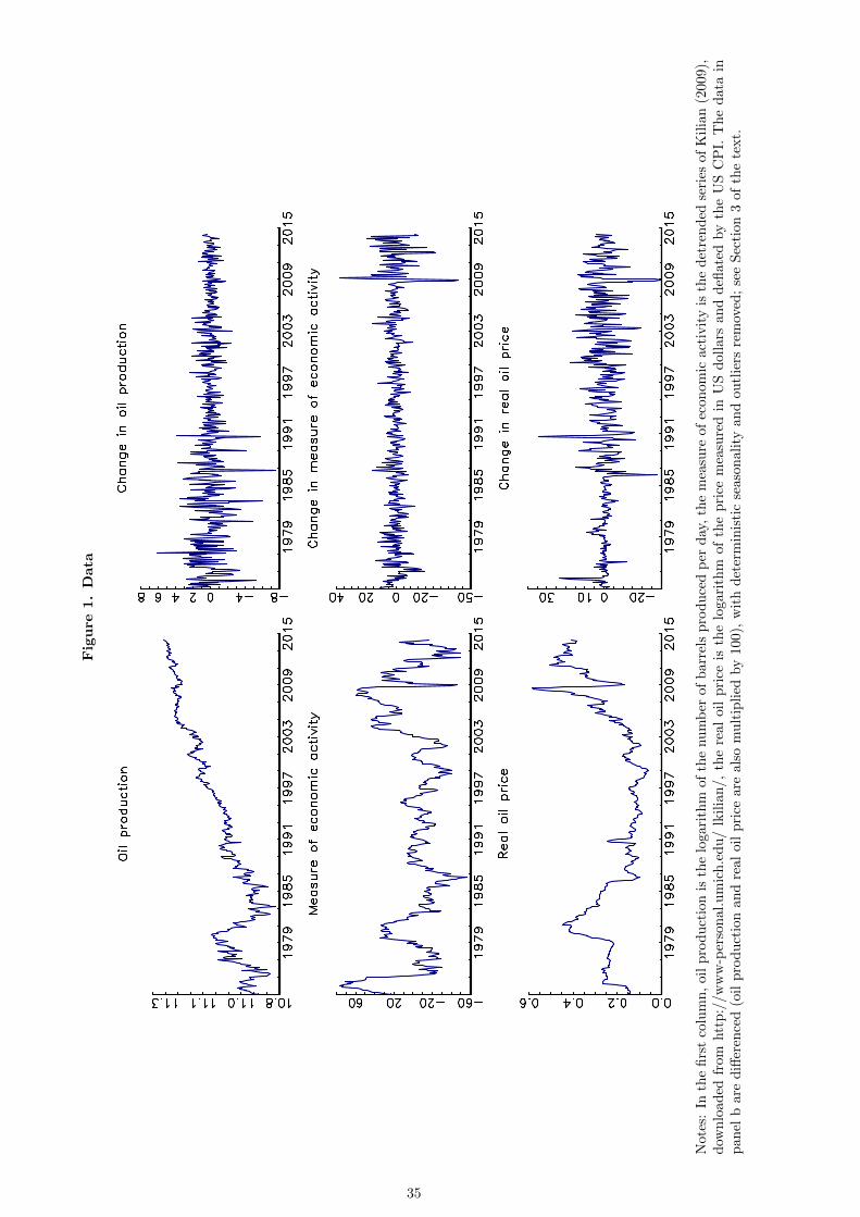
Fig

ure

1.

Data

Not

es:

Inth

efi

rst

colu

mn

,oi

lp

rod

uct

ion

isth

elo

gari

thm

ofth

enu

mb

erof

barr

els

pro

du

ced

per

day

,th

em

easu

reof

econ

om

icact

ivit

yis

the

det

ren

ded

seri

esof

Kil

ian

(2009),

dow

nlo

aded

from

htt

p:/

/ww

w-p

erso

nal

.um

ich

.ed

u/

lkil

ian

/,th

ere

al

oil

pri

ceis

the

logari

thm

of

the

pri

cem

easu

red

inU

Sd

oll

ars

an

dd

eflate

dby

the

US

CP

I.T

he

data

inp

anel

bar

ed

iffer

ence

d(o

ilp

rod

uct

ion

and

real

oil

pri

cear

eal

som

ult

ipli

edby

100),

wit

hd

eter

min

isti

cse

aso

nali

tyan

dou

tlie

rsre

mov

ed;

see

Sec

tion

3of

the

text.

35

Fig

ure

2.

Resp

on

seto

asu

pp

lysh

ock

01

02

0-4-3-2-101

Ja

n 7

5 -

De

c 8

0

Oil production

01

02

0-4-3-2-10

Ja

n 8

1 -

Ma

y 8

8

01

02

0-4-3-2-10

Ju

n 8

8 -

Oct 9

4

01

02

0-4-3-2-10

No

v 9

4 -

Fe

b 1

4

01

02

0-4-2024

Real activity

01

02

0-6-4-2024

01

02

0-1

0-505

01

02

0-1

0-505

01

02

0-1

0-505

10

Real price of oil

01

02

0-1

5

-10-505

10

01

02

0-4

0

-200

20

40

01

02

0-1

00

10

20

Not

es:

Eac

hgr

aph

show

sth

ecu

mu

late

dim

pu

lse

resp

onse

sto

ash

ock

of

aco

mm

on

magn

itu

de,

equ

al

toon

est

an

dard

dev

iati

on

esti

mate

dov

erth

ew

hole

sam

ple

wit

hn

ob

reak

s.E

ach

ofth

efo

ur

colu

mn

sre

pre

sents

asu

b-s

amp

leas

defi

ned

by

the

coeffi

cien

tb

reak

date

sof

Tab

le3.

Each

plo

tin

clu

des

on

e(b

lue

dash

edli

ne)

an

dtw

o(g

reen

das

hed

-dot

ted

lin

e)st

and

ard

dev

iati

onco

nfi

den

ceb

and

s(s

eete

xt)

.T

he

back

gro

un

dsh

ad

edare

as

pro

vid

eco

rres

pon

din

gco

nfi

den

cein

terv

als

aro

un

dth

ere

spon

ses

(dot

ted

lin

e)fo

ra

con

stan

tp

aram

eter

mod

eles

tim

ated

over

the

wh

ole

sam

ple

per

iod

.

36

Fig

ure

3.

Resp

on

seto

an

aggre

gate

dem

an

dsh

ock

01

02

0-6-4-202

Ja

n 7

5 -

De

c 8

0

Oil production

01

02

0-1

.5-1

-0.50

0.51

Ja

n 8

1 -

Ma

y 8

8

01

02

0-1

.5-1

-0.50

0.51

Ju

n 8

8 -

Oct 9

4

01

02

0-1

.5-1

-0.50

0.51

No

v 9

4 -

Fe

b 1

4

01

02

0-505

10

15

Real activity

01

02

005

10

15

01

02

005

10

15

01

02

005

10

15

01

02

0-1

0-505

10

15

Real price of oil

01

02

0-505

10

01

02

0-1

5

-10-505

10

01

02

0-202468

Note

s:See

Fig

ure

2.

.

37

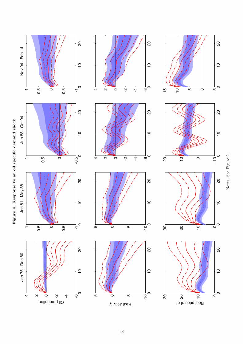
Fig

ure

4.

Resp

on

seto

an

oil

specifi

cd

em

an

dsh

ock

01

02

0-6-4-2024

Ja

n 7

5 -

De

c 8

0

Oil production

01

02

0-1

-0.50

0.51

Ja

n 8

1 -

Ma

y 8

8

01

02

0-0

.50

0.51

Ju

n 8

8 -

Oct 9

4

01

02

0-1

-0.50

0.51

No

v 9

4 -

Fe

b 1

4

01

02

0-1

0-505

Real activity

01

02

0-1

0-505

01

02

0-6-4-2024

01

02

0-6-4-2024

01

02

00

10

20

30

Real price of oil

01

02

00

10

20

30

01

02

0-1

00

10

20

01

02

0-505

10

15

Note

s:See

Fig

ure

2.

38