Embed Size (px)
Citation preview

Changes in Child Nutrition in IndiaA Decomposition ApproachNie, Peng; Rammohan, Anu; Gwozdz, Wencke; Sousa-Poza, Alfonso
Document VersionFinal published version
Published in:International Journal of Environmental Research and Public Health
DOI:10.3390/ijerph16101815
Publication date:2019
LicenseCC BY
Citation for published version (APA):Nie, P., Rammohan, A., Gwozdz, W., & Sousa-Poza, A. (2019). Changes in Child Nutrition in India: ADecomposition Approach. International Journal of Environmental Research and Public Health, 16(10), [1815].https://doi.org/10.3390/ijerph16101815
Link to publication in CBS Research Portal
General rightsCopyright and moral rights for the publications made accessible in the public portal are retained by the authors and/or other copyright ownersand it is a condition of accessing publications that users recognise and abide by the legal requirements associated with these rights.
Take down policyIf you believe that this document breaches copyright please contact us ([email protected]) providing details, and we will remove access tothe work immediately and investigate your claim.
Download date: 17. Nov. 2021

International Journal of
Environmental Research
and Public Health
Article
Changes in Child Nutrition in India:A Decomposition Approach
Peng Nie 1,* , Anu Rammohan 2, Wencke Gwozdz 3,4 and Alfonso Sousa-Poza 5
1 School of Economics and Finance, Xi’an Jiaotong University, Xi’an 710061, China2 Department of Economics, University of Western Australia, Perth, WA 6009, Australia;
[email protected] Institute of Household Sciences, Justus-Liebig-University, 35390 Giessen, Germany;
[email protected] Department of Intercultural Communication and Management, Centre for Corporate Social Responsibility,
Copenhagen Business School, 2000 Frederiksberg, Denmark5 Institute for Health Care & Public Management, University of Hohenheim, 70599 Stuttgart, Germany;
[email protected]* Correspondence: [email protected]; Tel.: +86-029-82656824
Received: 25 February 2019; Accepted: 18 May 2019; Published: 22 May 2019�����������������
Abstract: Background: Improvements in child health are a key indicator of progress towards thethird goal of the United Nations’ Sustainable Development Goals. Poor nutritional outcomes ofIndian children are occurring in the context of high economic growth rates. The aim of this paper isto conduct a comprehensive analysis of the demographic and socio-economic factors contributing tochanges in the nutritional status of children aged 0–5 years in India using data from the 2004–2005and 2011–2012 Indian Human Development Survey. Methods: To identify how much the differentsocio-economic conditions of households contribute to the changes observed in stunting, underweightand the Composite Index of Anthropometric Failure (CIAF), we employ both linear and non-lineardecompositions, as well as the unconditional quantile technique. Results: We find the incidenceof stunting and underweight dropping by 7 and 6 percentage points, respectively. Much of thisremarkable improvement is encountered in the Central and Western regions. A household’s economicsituation, as well as maternal body mass index and education, account for much of the change inchild nutrition. The same holds for CIAF in the non-linear decomposition. Although higher maternalautonomy is associated with a decrease in stunting and underweight, the contribution of maternalautonomy to improvements is relatively small. Conclusions: Household wealth consistently makesthe largest contribution to improvements in undernutrition. Nevertheless, maternal autonomy andeducation also play a relatively important role.
Keywords: child undernutrition; India; decomposition
1. Introduction
Improvements in child health are a key indicator of progress towards the third goal of the UnitedNations’ Sustainable Development Goals: A universal guarantee of a healthy life and well-being at allages. Undernutrition puts children at a greater risk of disease vulnerability, also adversely affects theirphysical, cognitive, and mental development [1,2], may adversely impact productivity in later life [3]and increase economic inequality [4].
Globally, India performs poorly across standard child nutritional measures [5]. For childmalnutrition, India ranked 114 out of 132 countries, just ahead of Afghanistan and Pakistan [6]. Datafrom India’s nationally representative National Family Health Survey (NFHS), from 1992–1993 to
Int. J. Environ. Res. Public Health 2019, 16, 1815; doi:10.3390/ijerph16101815 www.mdpi.com/journal/ijerph

Int. J. Environ. Res. Public Health 2019, 16, 1815 2 of 22
2015–2016, paint a bleak picture of child nutrition. Although the prevalence of stunting amongunder-five children decreased from 52% to 38% and underweight declined from 53% to 36% between1992 and 2016, prevalence is still alarmingly high [7]. In 2016, India had 62 million stunted children,accounting for 40% of the global share of stunting [7]. Large regional differences also exist with stuntingover 46% and 48% in the states of Uttar Pradesh (India’s most populated state) and Bihar [8].
These poor nutritional outcomes of Indian children are occurring in the context of high economicgrowth rates, but with low levels of maternal autonomy. Furthermore, a large body of empiricalresearch has linked greater maternal autonomy to better nutrition of children, particularly girls [9,10].An improvement in maternal autonomy is expected to improve a mother’s ability to make decisionsregarding her children’s health and nutrition; and a more autonomous mother is also likely to havegreater access to resources, may lead to the adoption of healthy and diversified diets, improve thenutritional content of diets, contribute to better food hygiene and sanitation, and thereby reduce therisk of infection and disease. Since undernutrition is the outcome of insufficient food intake andrepeated infectious diseases [11], it is imperative to understand the links between household-levelsocio-economic factors (and in particular the role of maternal autonomy) and the extent to which itmanifests into poor nutritional outcomes for children.
The aim of this paper, therefore, is to use the 2004–2005 and 2011–2012 data from the IndianHuman Development Survey (IHDS) to conduct a comprehensive analysis of the demographic andsocio-economic factors contributing to changes in the nutritional status (HAZ, WAZ and the CompositeIndex of Anthropometric Failure (CIAF)) of children aged 0–5 years in India. A special focus of ouranalysis is on the role that maternal autonomy plays in improving child undernutrition. Specifically,we address three key questions: (i) Have there been any changes in the nutritional status of childrenover the period 2004/2015–2011/2012? (ii) Do the changes differ across regions? (iii) What factorsare associated with the changing nutritional outcomes of children, and, in particular, what role doesmaternal autonomy play?
2. Prior studies
2.1. Socio-Economic Factors Associated with Child Undernutrition in India
A large body of research has used nationally representative secondary data to investigate thesocio-economic factors associated with poor child nutrition in India. These studies find an increasein inequalities for vulnerable groups such as girls and lower socio-economic individuals [12–16].Pathak and Singh [17] show that, over the period 1992–2006, the burden of undernutrition wasdisproportionately concentrated among poor children, with relatively better child nutrition in areaswhere households can access the Government funded Integrated Child Development Services (ICDS).Launched in 1975, the ICDS Program is a Government of India funded program aimed at improvingthe nutrition and health status of pre-school age children. In addition, Coffey [18] finds that state-levelvariation in neonatal mortality is associated with child heights. These findings are consistent withSubramanyam et al.’s [19] conclusion that over these 14 observation years, social disparities inundernutrition have either widened or stayed the same.
There is also empirical support for the role of maternal autonomy in influencing childnutrition [20,21]. In the Indian context, Shroff et al. [22] show that higher maternal autonomy(indicated by access to money and freedom to go to the market) is associated with a decreasedrisk of stunting among children aged below three years in the state of Andhra Pradesh. Similarly,Shroff et al. [23] find that maternal household decision-making autonomy is positively associatedwith weight-for-height (WHZ) and WAZ; while mobility autonomy is positively linked with HAZwhen adjusting for birth weight among infants aged 3–5 months. Similarly, Imai et al. [24] show thatmaternal autonomy (measured by whether she is allowed to go to market without her husband’spermission) is positively associated with HAZ and WAZ; and Arulampalam et al. [25] demonstratethat maternal autonomy (a composite measure of decision-making, mobility and financial autonomy)

Int. J. Environ. Res. Public Health 2019, 16, 1815 3 of 22
has a significant positive impact on HAZ, but is not associated with WHZ. Interestingly, Imai et al. [24]further indicate that maternal autonomy is only associated with HAZ at the low end of the conditionaldistribution. Nevertheless, one recent study [25] shows that maternal decision-making autonomyis not associated with any of undernutrition outcomes when adjusting for maternal and householdsocio-economic factors. Thus, empirical evidence is mixed although the majority of studies support anassociation between child nutrition and maternal autonomy.
Another strand of literature focuses on the role of poor health infrastructure. For example,Paul et al. [26] attribute the poor nutritional outcomes among Indian children to weak health systemsand a policy focus on children aged 3–6 years at the expense of those aged 0–2 years, although much ofa child’s growth occurs in the early years. Spears [27] and Hammer and Spears [28] further explainpoor child nutrition among Indian children in terms of sanitation, arguing that environmental threatsfrom open defecation and exposure to fecal germs reduce nutrient absorption, while exposure to earlylife disease leads to undernutrition, stunting, and diarrhea. Using data from the NFHS, Spears [29]shows that open defecation remains exceptionally widespread in India and sanitation has not improvedsubstantially despite rapid economic growth. Although these studies provide useful benchmarksfor assessing the links between socio-economic characteristics and child nutrition, they are based onNational Family and Health Survey (NFHS) and National Sample Survey (NSS) data sets that are overa decade old.
2.2. Applying Decomposition Analyses to Explain the Socio-Economic Factors Underlying ChildUndernutrition in India
The three major decomposition techniques, including Blinder-Oaxaca (BO) linear decomposition,nonlinear decomposition, and quantile-based decomposition, have been used in previous studies inIndia to analyze the gap in child undernutrition/health between certain groups (such as poor/non-poor,Muslims/Hindu, rural/urban). BO decomposition is used to decompose differences in a continuousvariable (e.g., child undernutrition outcome) into a part attributable to differences in characteristics(explained part or endowments part) and a part attributable to coefficients (unexplained part oreffects part). Nonlinear decomposition, in essence, employs an extension of the BO decomposition forbinary variables (e.g., underweight or stunting). BO decomposition is a mean-based approach, yetcovariate and coefficient contributions may differ at different parts of the distribution of undernutrition.Quantile-based decomposition is thus used to explore the contributions of covariates at differentquantiles of the outcome distribution. For example, Bhalotra et al. [30] apply a non-linear decompositiontechnique [31] to three waves of the NFHS (1992/1993, 1998/1999, and 2005/2006) to measure theHindu-Muslim gap in under-five child undernutrition. They show that the 29% difference in stuntingbetween these two groups is mainly attributable to maternal education, maternal age at parturition,and child’s birth year, while the 20% gap in wasting is primarily explainable by maternal educationand state of residence. Similarly, Kumar and Singh [32] apply the BO decomposition method to2005–2006 NFHS data to measure the gap in under-five child undernutrition between poor andnon-poor households in urban India. They identify the main contributing factors as underutilizationof health care services, poor maternal body mass index (BMI), and low levels of parental educationamong impoverished urbanists.
In a regression-based decomposition of the same datasets to assess (concentration index-based)inequalities in under-five child mortality and undernutrition outcomes, Chalasani [33] identifies wealthand mother’s education as the two largest contributors to severe stunting and severe underweightinequality over the 1992/1993–2005/2006 period. These results are supported by Kumar and Kumari [34],who use BO decomposition to show that household economic status (wealth score) and parentaleducation are the most significant contributors to the rural-urban gap in childhood undernutritionin India (measured using z-scores of weight-for-age). Similarly, using the 2005–2006 NFHS data,Mazumdar [35] identifies household wealth and mother’s education as the two largest contributors toinequality in child undernutrition in explaining the child undernutrition inequalities. Van de Poel and

Int. J. Environ. Res. Public Health 2019, 16, 1815 4 of 22
Speybroeck [36], in their earlier BO decomposition of 1998–1999 IDHS data, attribute the observedchild undernutrition gap among scheduled castes and scheduled tribes primarily to their lowerwealth, education level, and use of health care services. Cavatorta et al. [37] use Machado and Mata’sconditional quantile decomposition approach [38] to show that the surprisingly modest height-for-agedisparities across six Indian states can be explained by covariate differences in endowment effects.
Summing up, previous analyses of undernutrition changes in pre-school age Indian children pointto household economic status (particularly wealth) and maternal education as the two most importantcontributors. With few exceptions, however, this research predominantly uses BO decomposition,which can provide misleading estimates when the outcome variable is binary and explanatory variablesdiffer substantially across groups [39]. To the best of our knowledge, only two studies analyze childundernutrition using non-linear decomposition: Bhalotra et al. [30], who use the Fairlie method toidentify Hindu-Muslim disparities in under-five child mortality and undernutrition, and Cavatorta etal. [37], who employ Machado and Mata’s conditional quantile decomposition technique [38] to explorethe relative contributions of covariates and coefficients over the entire height-for-age distribution.Moreover, we are not aware of previous studies using the Fairlie non-linear decomposition to examineanthropometric failure differences between groups or over time, and the Machado and Mata’s method isnot extendable to a detailed decomposition for each determinant. We address both these research gapsand conduct a comprehensive analysis of the demographic and socio-economic factors contributing tochanges in the nutritional status (HAZ, WAZ and CIAF) of children aged 0–5 years in India using theIHDS data for 2004–2005 and 2011–2012.
3. Materials and Methods
3.1. Data
The data for this analysis are taken from the IHDS 2004–2005 and 2011–2012, a collaborativeresearch program between researchers from the National Council of Applied Economic Research,New Delhi, and the University of Maryland. This nationally representative multi-topic survey wasadministered to households in 1503 villages and 971 urban neighborhoods across India and thesample includes 384 districts out of a total of 593 identified in 2001 census. Villages and urban blocks(comprising of 150–200 households) form the primary sampling unit (PSU) from which the householdsare selected [40]. Urban and rural PSUs are selected using a different design. Specifically, to drawa random sample of urban households, all urban areas in a state are listed in the order of their sizewith the number of blocks drawn from each urban area allocated based on probability proportionalto size [40]. When the numbers of blocks for each urban area are fixed, the enumeration blocks arethen selected randomly with the assistance from Registrar General of India. Drawing on these CensusEnumeration Blocks of about 150–200 households, a complete household listing is conducted anda household sample of 15 households is selected within each block. For sampling purposes, somesmaller states are merged with nearby larger states. Nevertheless, the rural sample encompassesabout half the households that are interviewed initially by NCAER in 1993–1994 in a survey titledHuman Development Profile of India (HDPI) and the other half of the samples are drawn from bothdistricts surveyed in HDPI as well as from the districts located in the states and union territories notcovered in HDPI [40]. The first phase, IHDS-I (2004–2005), comprised two one-hour interviews witheach household on topics such as health status, education, employment, economic status, marriage,fertility, gender relations, and social capital. The second phase, IHDS-II, was conducted between2011–2012. A detailed description of sampling design and data quality is available in Reference [40].All individual- and household-level data are available for public use [41].
Our sample is restricted to those households with children born in the five years prior to thesurvey, where information was available on all our variables of interest. Because data on certainoutcome variables of interest are limited, our final pooled sample contains 6445 observations forstunting, 7634 observations for underweight, and 5693 observations for the CIAF.
Int. J. Environ. Res. Public Health 2019, 16, 1815 5 of 22
3.2. Study Variables
3.2.1. Dependent Variables
In keeping with the World Health Organization’s reference standards [42], we measure children’snutritional outcomes conventionally using z-scores of height-for-age (HAZ) and weight for age (WAZ).According to Waterlow et al. [43], the height-for-age z-score, expressed in standard deviations fromthe reference population mean, is a good indicator of nutritional status. Whereas HAZ measureslong-term nutrition by showing the cumulative effects of growth deficiency (often associated withchronic insufficient food intake, frequent infections, sustained incorrect feeding practices, and/or lowsocio-economic family status), WAZ reflects both acute and chronic undernutrition, making it a bettersingle indicator of childhood undernutrition [44].
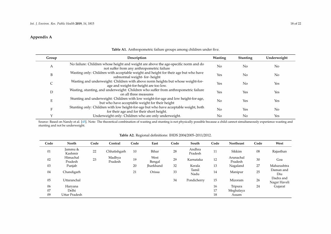
Children with z-score values below −2 (below −3) of the reference population are consideredundernourished (severely undernourished) [42]. However, because these conventional undernutritionmeasures reflect different aspects of anthropometric failure, they cannot individually determine theoverall prevalence of child undernutrition in a population, and may underestimate the true extent ofundernutrition, primarily due to the overlapping of children into multiple categories of anthropometricfailure [45–48]. For instance, underweight cannot identify children who are suffering from underweightcombined with stunting and/or wasting [46,47]. We address this shortcoming using Svedberg’s [48]CIAF, an aggregated single anthropometric proxy for the overall estimation of malnourished children.In our analysis, we combine Nandy et al.’s [45] Group Y, underweight only, with six of Svedberg’sgroups [48]: Group A, no failure; Group B, wasting only; Group C, wasting and underweight; GroupD, wasting, stunting, and underweight; Group E, stunting and underweight; and Group F, stuntingonly (see Table A1 for a detailed classification). CIAF is thus a binary variable for which 0 indicates nofailure, and 1 signals one or more anthropometric failures.
3.2.2. Explanatory Variables
Maternal characteristics. We control for mother’s education using four categories: No education,primary, secondary, tertiary and above. As a proxy for mother’s health, we include her BMI measuredin kg/m2 (categorizing into three groups: Underweight for BMI < 18.5, normal for 18.5 ≤ BMI ≤ 24.9and overweight/obesity for BMI ≥ 25).
Economic characteristics. A household’s economic status is measured using the household wealthindex, which is a categorical variable divided into five population quintiles from the poorest 20% tothe wealthiest 20% of households [49]. This index is calculated with Principle Component Analyses(PCA) using 33 dichotomous items measuring household ownership of assets and housing quality.Relative to income and consumption, this measure of wealth is less volatile and thus arguably a betterlong-run measure of household economic status.
Maternal autonomy. A key advantage of our dataset is the rich array of attitudinal questions thatare available on married women’s decision-making authority in the household. Autonomy is regardedas a multidimensional construct, encompassing dimensions such as the ability to make purchases,control over resources, decision-making autonomy both relating to own health care or child’s medicalneeds [50]. We therefore categorize maternal autonomy into:
• Decision-making autonomy: A female respondent (child’s mother) is assumed to havedecision-making autonomy if she was involved in decision-making either on her own or inconjunction with another household member on: (i) What is to be cooked, (ii) making expensivepurchases, (iii) the number of children to have, and (iv) children’s medical needs (decide what todo when a child falls sick).
• Mobility autonomy: The child’s mother is assumed to have mobility autonomy if she can go on herown: (i) To visit relatives/friends, (ii) to the local health center, and (iii) to the local grocery store.
Int. J. Environ. Res. Public Health 2019, 16, 1815 6 of 22
These individual responses are coded as binary indicators which we use to construct two factors:Maternal autonomy in decision-making and mobility using PCA.
Hygiene characteristics. We include three binary variables that capture the level of sanitation andhygiene practiced in the household: Drinking water source (1 if the household’s drinking water ispiped or supplied by tube well or hand pump, 0 otherwise), access to a flushing toilet (1 = yes, 0 = no),and hand-washing behavior (1 = yes, 0 = no).
Regional characteristics. The 24 Indian states are classified into six regions as per the regionaldefinitions used in the IHDS data (see Table A2). These are: North (comprising of the states of Jammuand Kashmir, Himachal Pradesh, Punjab, Chandigarh, Uttaranchal, Uttar Pradesh, Haryana and Delhi);Central (Chhattisgarh and Madhya Pradesh); East (Bihar, West Bengal, Jharkhand, Odisha); South(Andhra Pradesh, Karnataka, Kerala, Tamil Nadu and Pondicherry); North East (Sikkim, ArunachalPradesh, Nagaland, Manipur, Mizoram, Tripura, Meghalaya and Assam); and West (Rajasthan, Goa,Maharashtra, Daman and Diu, Dadar and Nagar Haveli and Gujarat). The descriptive analysis ofregional changes in child nutrition are based on these six regions.
Other characteristics. Our specifications also include controls for child’s age (in years) and gender(1 = male and 0 = female), father’s education levels (a categorical variable, 1 = no education, 2 = primary,3 = secondary and 4 = tertiary and above), religion (a categorical variable, 1 = Hindu, 2 = Muslim and3 = others), caste (a categorical variables, 1 = other, 2 = other backward and 3 = scheduled caste/tribe)and a binary variable for rural residence (1 = rural and 0 = urban).
3.3. Estimation Procedure
Blinder-Oaxaca (BO) decomposition. We use BO decomposition to explain changes in the nutritionalmeasures HAZ and WAZ as a function of selected explanatory factors. The BO decomposition quantifiesthe distribution differences of factors that explain the average gap, and also identifies differencesin these factors’ effects [51]. The total difference in mean z-scores of our three measures of childundernutrition can be decomposed as follows:
Y2011/12
−Y2004/05
=(X
2011/12−X
2004/05)β̂2011/12 + X
2004/05(β̂2011/12
− β̂2004/05)
(1)
where Xi
is a vector of the averaged values of the independent variables and β̂i is a vector of thecoefficient estimates for wave i (here, i = 2004/2005, 2011/2012).
Re-centred influence function regression (RIFR) decomposition. Because covariate and coefficientcontributions may differ between the median and tails of the childhood undernutrition distribution,we use RIFR decomposition [52] to investigate the contributions of demographic and socio-economiccharacteristics at different quantiles of the unconditional marginal distribution. The RIFR methodinvolves a two-step procedure: First, we calculate an influence function (IF) at each quantile τ of thedistribution of the outcome variable (z-score of child undernutrition), as follows:
RIF(zscore; qτ) = qτ + (τ− 1[zscore ≤ qτ])/ fzscore(qτ) (2)
where qτ represents the unconditional τth quantile of the z-score, fzscore(qτ) is the unconditional densityof the z-score at the τth quantile, and 1[zscore ≤ qτ] is an indicator function for whether the outcomevariable is smaller or equal to the τth quantile. For each quantile, the coefficient on X for waves2004/2005 and 2011/2012 are then estimated by regressing the RIF on X:
qwave, τ = EX[E[
ˆRIF(zscore; qwave, τ)∣∣∣Xwave
]]= E[Xwave]θ̂wave,τ (3)
where qwave, τ is the unconditional τth quantile of the z-score for wave 2004/05 and 2011/12, respectively.θ̂wave,τ is the coefficient of the unconditional quantile regression, which captures the marginal effect ofa change in the distribution of X on the unconditional quantile of the z-score.

Int. J. Environ. Res. Public Health 2019, 16, 1815 7 of 22
In the second step, we employ the BO decomposition strategy at different quantiles (25%, 50%,and 75%) calculated by the RIFR:
∆̂τzscore =[
ˆRIF(zscore2011/12; q2011/12, τ
)]−
[ˆRIF
(zscore2004/05; q2004/05, τ
)](4)
∆̂τzscore =(X2011/12 −X2004/05
)θ̂2011/12,τ + X2004/05
(θ̂2011/12,τ − θ̂2004/05,τ
)(5)
Both the explained and unexplained parts are then decomposed into the contributions of eachcovariate at the τth quantile in Equation (5), which is in effect analogous to the BO decomposition inEquation (1).
Fairlie’s (1999) non-linear decomposition. Applying standard BO decomposition to a linear probabilitymodel provides misleading estimates for binary dependent variables, particularly if the groupdifferences for an influential independent variable are relatively large [39]. It is therefore preferable toapply a relatively straightforward simulation technique for non-linear decomposition. Accordingly,we estimate the contributions of socio-economic and demographic factors to identified differences in ourkey undernutrition indicators by employing a non-linear decomposition approach for binary dependentvariables. Stunting, underweight, and CIAF are the dependent variables, so the decomposition for thenon-linear equation, Y = F
(Xβ̂
), can be expressed as:
Y2011/12
−Y2004/05
=
(∑N2011/12
i=1F(X2011/12
i β̂2004/05)N2011/12
−∑N2004/05
i=1F(X2004/05
i β̂2004/05)N2004/05
)−
∑N2011/12
i=1F(X2011/12
i β̂2011/12)N2011/12
−∑N2011/12
i=1F(X2011/12
i β̂2004/05)N2011/12
)(6)
where N j denotes the sample size of each wave (j = 2004/2005, 2011/2012). The function F(.) representsa probit model. Two aspects are worth noting: First, the BO decomposition in Equation (1) is a specialcase of Equation (6) where F(Xiβ) = Xiβ. Second, in Equations (1) and (6), the first (explained) term onthe right indicates the contribution resulting from a difference in the distribution of the determinant ofX, and the second (unexplained) term refers to the part attributable to a difference in the effect of thedeterminants. Equally noteworthy, the second term captures all the potential effects of differences inunobservables [39]. In keeping with previous research using decomposition, we focus on the explainedterms and their disaggregated contribution for individual covariates, which result primarily fromthe difficulty of interpreting the unexplained part [53]. The contribution of a variable is given by theaverage change in the function if that variable is changed while all other variables remain the same.For severe childhood undernutrition in terms of HAZ and WAZ, we use the same specification as inEquation (6).
One potential concern related to Fairlie’s sequential decomposition is path dependence, thepossibility that changing the order of variables in the decomposition may produce differentresults [39,54]. We therefore test the sensitivity of decomposition estimates to variable re-orderingby randomizing their order in the decomposition [39] using 1000 replications, the minimum numberrecommended for most applications [39]. As a robustness check, we also perform an analysis using5000 replications. These results are not reported here but are available on request.
When reporting the decomposition results for these three decomposition methods, we categorizethe disaggregated contributions of the determinants in the explained part into five main dimensionsdepicted above, namely: Maternal autonomy, maternal characteristics, household economic status,hygiene, and other.
Int. J. Environ. Res. Public Health 2019, 16, 1815 8 of 22
4. Results
4.1. Descriptive Statistics
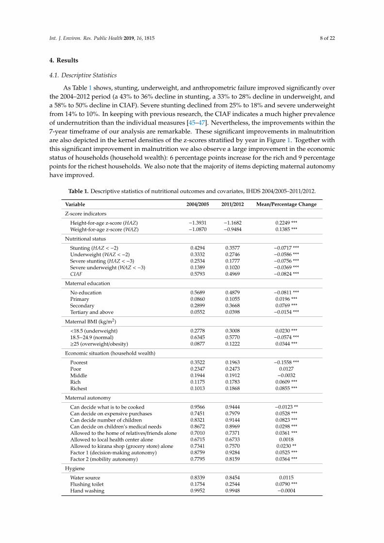
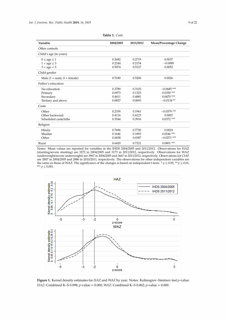
As Table 1 shows, stunting, underweight, and anthropometric failure improved significantly overthe 2004–2012 period (a 43% to 36% decline in stunting, a 33% to 28% decline in underweight, anda 58% to 50% decline in CIAF). Severe stunting declined from 25% to 18% and severe underweightfrom 14% to 10%. In keeping with previous research, the CIAF indicates a much higher prevalenceof undernutrition than the individual measures [45–47]. Nevertheless, the improvements within the7-year timeframe of our analysis are remarkable. These significant improvements in malnutritionare also depicted in the kernel densities of the z-scores stratified by year in Figure 1. Together withthis significant improvement in malnutrition we also observe a large improvement in the economicstatus of households (household wealth): 6 percentage points increase for the rich and 9 percentagepoints for the richest households. We also note that the majority of items depicting maternal autonomyhave improved.
Table 1. Descriptive statistics of nutritional outcomes and covariates, IHDS 2004/2005–2011/2012.
Variable 2004/2005 2011/2012 Mean/Percentage Change
Z-score indicators
Height-for-age z-score (HAZ) −1.3931 −1.1682 0.2249 ***Weight-for-age z-score (WAZ) −1.0870 −0.9484 0.1385 ***
Nutritional status
Stunting (HAZ < −2) 0.4294 0.3577 −0.0717 ***Underweight (WAZ < −2) 0.3332 0.2746 −0.0586 ***Severe stunting (HAZ < −3) 0.2534 0.1777 −0.0756 ***Severe underweight (WAZ < −3) 0.1389 0.1020 −0.0369 ***CIAF 0.5793 0.4969 −0.0824 ***
Maternal education
No education 0.5689 0.4879 −0.0811 ***Primary 0.0860 0.1055 0.0196 ***Secondary 0.2899 0.3668 0.0769 ***Tertiary and above 0.0552 0.0398 −0.0154 ***
Maternal BMI (kg/m2)
<18.5 (underweight) 0.2778 0.3008 0.0230 ***18.5−24.9 (normal) 0.6345 0.5770 −0.0574 ***≥25 (overweight/obesity) 0.0877 0.1222 0.0344 ***
Economic situation (household wealth)
Poorest 0.3522 0.1963 −0.1558 ***Poor 0.2347 0.2473 0.0127Middle 0.1944 0.1912 −0.0032Rich 0.1175 0.1783 0.0609 ***Richest 0.1013 0.1868 0.0855 ***
Maternal autonomy
Can decide what is to be cooked 0.9566 0.9444 −0.0123 **Can decide on expensive purchases 0.7451 0.7979 0.0528 ***Can decide number of children 0.8321 0.9144 0.0823 ***Can decide on children’s medical needs 0.8672 0.8969 0.0298 ***Allowed to the home of relatives/friends alone 0.7010 0.7371 0.0361 ***Allowed to local health center alone 0.6715 0.6733 0.0018Allowed to kirana shop (grocery store) alone 0.7341 0.7570 0.0230 **Factor 1 (decision-making autonomy) 0.8759 0.9284 0.0525 ***Factor 2 (mobility autonomy) 0.7795 0.8159 0.0364 ***
Hygiene
Water source 0.8339 0.8454 0.0115Flushing toilet 0.1754 0.2544 0.0790 ***Hand washing 0.9952 0.9948 −0.0004
Int. J. Environ. Res. Public Health 2019, 16, 1815 9 of 22
Table 1. Cont.
Variable 2004/2005 2011/2012 Mean/Percentage Change
Other controls
Child’s age (in years)
0 ≤ age ≤ 1 0.2682 0.2719 0.00371 < age ≤ 3 0.2244 0.2154 −0.00893 < age < 5 0.5074 0.5127 0.0052
Child gender
Male (1 = male, 0 = female) 0.5180 0.5206 0.0026
Father’s education
No education 0.3789 0.3103 −0.0685 ***Primary 0.0973 0.1323 0.0350 ***Secondary 0.4411 0.4881 0.0470 ***Tertiary and above 0.0827 0.0693 −0.0134 **
Caste
Other 0.2339 0.1961 −0.0379 ***Other backward 0.4116 0.4123 0.0007Scheduled caste/tribe 0.3544 0.3916 0.0372 ***
Religion
Hindu 0.7696 0.7720 0.0024Muslim 0.1646 0.1893 0.0246 ***Other 0.0658 0.0387 −0.0271 ***
Rural 0.6420 0.7221 0.0801 ***
Notes: Mean values are reported for variables in the IHDS 2004/2005 and 2011/2012. Observations for HAZ(stunting/severe stunting) are 3272 in 2004/2005 and 3173 in 2011/2012, respectively. Observations for WAZ(underweight/severe underweight) are 3967 in 2004/2005 and 3667 in 2011/2012, respectively. Observations for CIAFare 2807 in 2004/2005 and 2886 in 2010/2011, respectively. The observations for other independent variables arethe same as those of WAZ. The significance of the changes is based on independent t-tests. * p ≤ 0.05, ** p ≤ 0.01,*** p ≤ 0.001.
Int. J. Environ. Res. Public Health 2019, 16, x 9 of 22
Father’s education No education 0.3789 0.3103 −0.0685 *** Primary 0.0973 0.1323 0.0350 *** Secondary 0.4411 0.4881 0.0470 *** Tertiary and above 0.0827 0.0693 −0.0134 ** Caste Other 0.2339 0.1961 −0.0379 *** Other backward 0.4116 0.4123 0.0007 Scheduled caste/tribe 0.3544 0.3916 0.0372 *** Religion Hindu 0.7696 0.7720 0.0024 Muslim 0.1646 0.1893 0.0246 *** Other 0.0658 0.0387 −0.0271 *** Rural 0.6420 0.7221 0.0801 ***
Notes: Mean values are reported for variables in the IHDS 2004/2005 and 2011/2012. Observations for HAZ (stunting/severe stunting) are 3272 in 2004/2005 and 3173 in 2011/2012, respectively. Observations for WAZ (underweight/severe underweight) are 3967 in 2004/2005 and 3667 in 2011/2012, respectively. Observations for CIAF are 2807 in 2004/2005 and 2886 in 2010/2011, respectively. The observations for other independent variables are the same as those of WAZ. The significance of the changes is based on independent t-tests. * p ≤ 0.05, ** p ≤ 0.01, *** p ≤ 0.001.
Figure 1. Kernel density estimates for HAZ and WAZ by year. Notes: Kolmogrov–Smirnov test p-value: HAZ: Combined K–S 0.098; p-value = 0.000; WAZ: Combined K–S 0.062; p-value = 0.000.
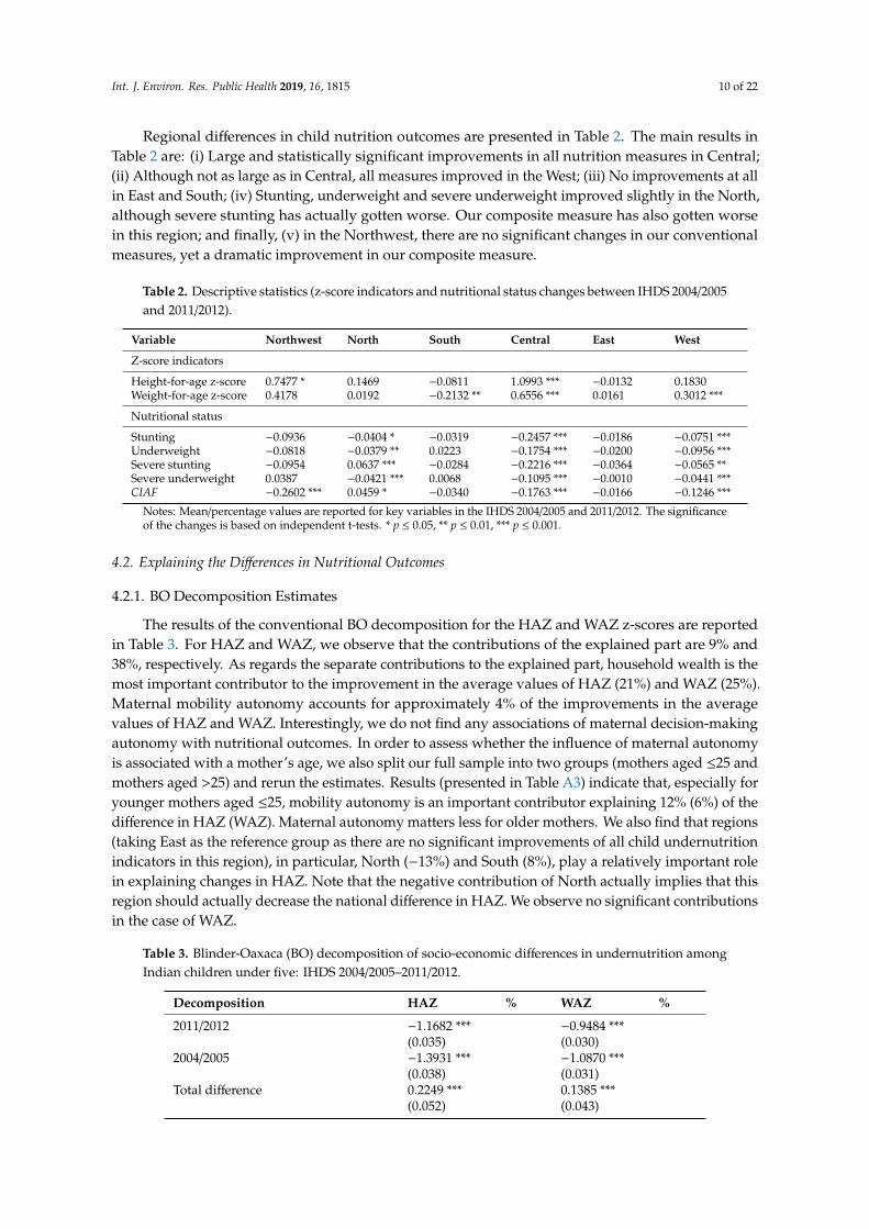
Regional differences in child nutrition outcomes are presented in Table 2. The main results in Table 2 are: (i) Large and statistically significant improvements in all nutrition measures in Central; (ii) Although not as large as in Central, all measures improved in the West; (iii) No improvements at all in East and South; (iv) Stunting, underweight and severe underweight improved slightly in the North, although severe stunting has actually gotten worse. Our composite measure has also gotten
Figure 1. Kernel density estimates for HAZ and WAZ by year. Notes: Kolmogrov–Smirnov test p-value:HAZ: Combined K–S 0.098; p-value = 0.000; WAZ: Combined K–S 0.062; p-value = 0.000.
Int. J. Environ. Res. Public Health 2019, 16, 1815 10 of 22
Regional differences in child nutrition outcomes are presented in Table 2. The main results inTable 2 are: (i) Large and statistically significant improvements in all nutrition measures in Central;(ii) Although not as large as in Central, all measures improved in the West; (iii) No improvements at allin East and South; (iv) Stunting, underweight and severe underweight improved slightly in the North,although severe stunting has actually gotten worse. Our composite measure has also gotten worsein this region; and finally, (v) in the Northwest, there are no significant changes in our conventionalmeasures, yet a dramatic improvement in our composite measure.
Table 2. Descriptive statistics (z-score indicators and nutritional status changes between IHDS 2004/2005and 2011/2012).
Variable Northwest North South Central East West
Z-score indicators
Height-for-age z-score 0.7477 * 0.1469 −0.0811 1.0993 *** −0.0132 0.1830Weight-for-age z-score 0.4178 0.0192 −0.2132 ** 0.6556 *** 0.0161 0.3012 ***
Nutritional status
Stunting −0.0936 −0.0404 * −0.0319 −0.2457 *** −0.0186 −0.0751 ***Underweight −0.0818 −0.0379 ** 0.0223 −0.1754 *** −0.0200 −0.0956 ***Severe stunting −0.0954 0.0637 *** −0.0284 −0.2216 *** −0.0364 −0.0565 **Severe underweight 0.0387 −0.0421 *** 0.0068 −0.1095 *** −0.0010 −0.0441 ***CIAF −0.2602 *** 0.0459 * −0.0340 −0.1763 *** −0.0166 −0.1246 ***
Notes: Mean/percentage values are reported for key variables in the IHDS 2004/2005 and 2011/2012. The significanceof the changes is based on independent t-tests. * p ≤ 0.05, ** p ≤ 0.01, *** p ≤ 0.001.
4.2. Explaining the Differences in Nutritional Outcomes
4.2.1. BO Decomposition Estimates
The results of the conventional BO decomposition for the HAZ and WAZ z-scores are reportedin Table 3. For HAZ and WAZ, we observe that the contributions of the explained part are 9% and38%, respectively. As regards the separate contributions to the explained part, household wealth is themost important contributor to the improvement in the average values of HAZ (21%) and WAZ (25%).Maternal mobility autonomy accounts for approximately 4% of the improvements in the averagevalues of HAZ and WAZ. Interestingly, we do not find any associations of maternal decision-makingautonomy with nutritional outcomes. In order to assess whether the influence of maternal autonomyis associated with a mother’s age, we also split our full sample into two groups (mothers aged ≤25 andmothers aged >25) and rerun the estimates. Results (presented in Table A3) indicate that, especially foryounger mothers aged ≤25, mobility autonomy is an important contributor explaining 12% (6%) of thedifference in HAZ (WAZ). Maternal autonomy matters less for older mothers. We also find that regions(taking East as the reference group as there are no significant improvements of all child undernutritionindicators in this region), in particular, North (−13%) and South (8%), play a relatively important rolein explaining changes in HAZ. Note that the negative contribution of North actually implies that thisregion should actually decrease the national difference in HAZ. We observe no significant contributionsin the case of WAZ.
Table 3. Blinder-Oaxaca (BO) decomposition of socio-economic differences in undernutrition amongIndian children under five: IHDS 2004/2005–2011/2012.
Decomposition HAZ % WAZ %
2011/2012 −1.1682 *** −0.9484 ***(0.035) (0.030)
2004/2005 −1.3931 *** −1.0870 ***(0.038) (0.031)
Total difference 0.2249 *** 0.1385 ***(0.052) (0.043)

Int. J. Environ. Res. Public Health 2019, 16, 1815 11 of 22
Table 3. Cont.
Decomposition HAZ % WAZ %
Explained 0.0195 9 0.0525 ** 38(0.027) (0.024)
Unexplained 0.2054 *** 91 0.0860 ** 62(0.054) (0.043)
Explained part
Mother’s decision-making autonomy −0.0028 −1 −0.0011 −1(0.005) (0.003)
Mother’s mobility autonomy 0.0099 *** 4 0.0061 ** 4(0.004) (0.002)
Mother’s characteristics 0.0033 1 0.0161 ** 12(0.007) (0.007)
Economic situation 0.0475 *** 21 0.0345 *** 25(0.017) (0.013)
Hygiene 0.0089 4 0.0027 2(0.007) (0.005)
Northwest −0.0024 −1 −0.0011 −1(0.003) (0.001)
North −0.0300 *** −13 0.0025 2(0.007) (0.004)
South 0.0183 *** 8 0.0026 2(0.007) (0.004)
Central −0.0040 −2 −0.0027 −2(0.005) (0.003)
West 0.0014 1 −0.0009 −1(0.002) (0.002)
Others −0.0304 * −14 −0.0062 −4(0.016) (0.017)
N 6445 7634
Note: The dependent variables are the z-scores of height-for-age (HAZ) and weight-for-age (WAZ). Groups in theexplained part are mother’s characteristics (mother’s BMI; mother’s education), household economic situation(household wealth); hygiene (water source; flushing toilet; and hand washing); and others (child age; child gender;father's education; caste; religion; rural resident) and 5 regional binary variables. Standard errors are in parentheses.* p ≤ 0.05, ** p ≤ 0.01, *** p ≤ 0.001.
4.2.2. RIFR Decomposition Estimates
The results of the RIFR decomposition are presented in Table 4. We observe large differencesin malnutrition between the two surveys, particularly at the bottom end of the distributions, andinsignificant at the upper end (75th quantile). The decomposition analysis produces three noteworthyfindings: First, household wealth makes the largest contribution to the overall explained part for bothHAZ and WAZ (panels A and B, respectively), especially at the lower parts of the distribution (for HAZ,25th quantile: 25%, 50th quantile: 37%; for WAZ, 25th quantile: 22%, 50th quantile: 61%). Second, inthe lowest part of the distribution (25th quantile) of HAZ (Panel A), about 4% of the improvements canbe explained with maternal characteristics of BMI and education and about 5% and 6% in the medianquantile respectively. With regards to WAZ (Panel B), the contribution of maternal characteristics tothe explained component becomes even larger, ranging from 6% at 25th quantile to 16% at the median.Third, mobility autonomy’s contribution to the improvement in HAZ ranges from 4% to 5% at the 25thand 50th quantiles, respectively (panel A). Additionally, we also find that regions (North and South)also make a relatively large contribution to the overall explained part for HAZ, though the relativecontributions of North and South are much larger at the median level than these at the 25th quantile(North: 14% versus -6%; South: 15% versus 5%). However, we only observe a larger contribution ofSouthern region (10%) to the overall explained part for WAZ at the median level.

Int. J. Environ. Res. Public Health 2019, 16, 1815 12 of 22
Table 4. RIFR decomposition of socio-economic differences in HAZ and WAZ among Indian childrenunder five: IHDS 2004/2005–2011/2012.
Panel A: HAZ 25th % 50th % 75th %
2011/2012 −2.5250 *** −1.3954 *** 0.0343(0.058) (0.038) (0.049)
2004/2005 −2.9957 *** −1.6054 *** −0.0186(0.044) (0.047) (0.046)
Total difference 0.4707 *** 0.2101 *** 0.0529(0.072) (0.061) (0.072)
Explained 0.1179 *** 25 0.0778 *** 37 −0.0521(0.036) (0.027) (0.033)
Unexplained 0.3527 *** 75 0.1323 ** 63 0.1050(0.081) (0.063) (0.075)
Explained part
Mother's decision-making autonomy −0.0125 * −3 −0.0041 −2(0.007) (0.006)
Mother's mobility autonomy 0.0174 *** 4 0.0112 ** 5(0.006) (0.005)
Mother’s characteristics 0.0209 ** 4 0.0118 6(0.009) (0.009)
Economic situation 0.1156 *** 25 0.0807 *** 38(0.025) (0.020)
Hygiene 0.0085 2 0.0054 3(0.009) (0.010)
Northwest 0.0032 1 −0.0028 1(0.004) (0.004)
North −0.0292 *** −6 −0.0290 *** 14(0.009) (0.008)
South 0.0214 ** 5 0.0320 *** 15(0.009) (0.007)
Central 0.0108 2 −0.0012 −1(0.007) (0.006)
West −0.0008 0 0.0019 1(0.002) (0.002)
Others −0.0374 ** −7 −0.0280 * −14(0.015) (0.015)
N 6445 6445 6445
Panel B: WAZ 25th % 50th % 75th %
2011/2012 −2.0814 *** −1.1336 *** −0.1021 **(0.031) (0.026) (0.040)
2004/2005 −2.3938 *** −1.2779 *** −0.1362 ***(0.031) (0.041) (0.041)
Total difference 0.3123 *** 0.1444 *** 0.0341(0.046) (0.050) (0.060)
Explained 0.0696 *** 22 0.0883 *** 61 0.0173(0.021) (0.026) (0.029)
Unexplained 0.2428 *** 78 0.0561 39 0.0168(0.050) (0.054) (0.061)
Explained part
Mother’s decision-making autonomy −0.0038 −1 0.0028 2(0.004) (0.004)
Mother’s mobility autonomy 0.0025 1 0.0042 * 3(0.002) (0.002)
Mother’s characteristics 0.0198*** 6 0.0226 *** 16(0.007) (0.008)

Int. J. Environ. Res. Public Health 2019, 16, 1815 13 of 22
Table 4. Cont.
Panel A: HAZ 25th % 50th % 75th %
Economic situation 0.0500 *** 16 0.0722 *** 50(0.015) (0.015)
Hygiene 0.0023 1 −0.0055 −4(0.005) (0.005)
Northwest 0.0009 0 0.0011 1(0.001) (0.002)
North 0.0062 2 −0.0019 −1(0.004) (0.005)
South 0.0042 1 0.0140 *** 10(0.004) (0.005)
Central 0.0016 1 −0.0127 *** −9(0.004) (0.004)
West −0.0002 0 0.0052 * 4(0.002) (0.003)
Others −0.0138 −4 −0.0136 −9(0.010) (0.016)
N 7634 7634 7634
Note: The dependent variables are the z-scores of height-for-age (HAZ) and weight-for-age (WAZ). Groups in theexplained part are mother’s characteristics (mother’s BMI; mother’s education), household economic situation(household wealth); hygiene (water source; flushing toilet; and hand washing); and others (child age; child gender;father's education; caste; religion; rural resident) and 5 regional binary variables. Standard errors are in parentheses.Standard errors are in parentheses. * p ≤ 0.05, ** p ≤ 0.01, *** p ≤ 0.001.
4.2.3. Fairlie Nonlinear Decomposition Estimates
The results of Fairlie non-linear decomposition are presented in Table 5. As can be seen,the contributions of the explained part vary substantially for the different measures of childundernutrition: 12% for stunting, 8% for underweight, and 40% for the CIAF. For the individualcontribution of each dimension in the explained part, household economic status (householdwealth) uniformly explains the largest proportion of improvements in stunting, underweight, andanthropometric failure, with contributions of 20%, 24%, and 19%, respectively. Likewise, maternalcharacteristics (including maternal BMI and education) explain 3% of stunting, 5% of underweight, 7%of anthropometric failure. Maternal mobility autonomy accounts for about 3% of the improvement inall measures. We also find that regions (especially South) play an important role in accounting for theimprovements in stunting and CIAF (stunting: 7%; CIAF: 11%). In addition, the Southern region alsocontributes to around 3% of the improvement of underweight.
Table 5. Non-linear decomposition of socio-economic differences in stunting, underweight and CIAFamong Indian children under five: IHDS 2004/2005–2011/2012.
Decomposition Stunting % Underweight % CIAF %
2011/2012 0.3577 0.2746 0.49382004/2005 0.4207 0.3182 0.5793Total difference −0.0630 *** −0.0436 *** −0.0855 ***Explained −0.0074 12 −0.0033 8 −0.0340 40Unexplained −0.0556 88 −0.0403 92 −0.0515 60
Explained part
Mother’s decision-making autonomy 0.0001 0 0.0013 −3 0.0004 0(0.001) (0.001) (0.001)
Mother’s mobility autonomy −0.0019 *** 3 −0.0010 ** 2 −0.0015 * 2(0.001) (0.000) (0.001)
Mother’s characteristics −0.0022 ** 3 −0.0021 ** 5 −0.0061 *** 7(0.001) (0.001) (0.002)

Int. J. Environ. Res. Public Health 2019, 16, 1815 14 of 22
Table 5. Cont.
Decomposition Stunting % Underweight % CIAF %
Economic situation −0.0123 *** 20 −0.0106 *** 24 −0.0164 *** 19(0.004) (0.003) (0.004)
Hygiene −0.0021 3 0.0002 0 −0.0035 * 4(0.002) (0.001) (0.002)
Northwest 0.0007 −1 0.00004 0 −0.0029 *** 3(0.001) (0.000) (0.001)
North 0.0048 *** −8 −0.0011 3 0.0030 * −4(0.001) (0.001) (0.002)
South −0.0043 *** 7 −0.0013 3 −0.0092 *** 11(0.001) (0.001) (0.002)
Central −0.0007 1 −0.0002 1 0.0022 ** −3(0.001) (0.001) (0.001)
West −0.0001 0 0.0002 0 −0.0007 ** 1(0.000) (0.001) (0.000)
Others 0.0104 *** −17 0.0113 *** −26 0.0008 −1(0.002) (0.002) (0.002)
Number of replications 1000 1000 1000
Note: The dependent variable is a dummy for whether the respondent is suffering or has suffered from stunting,underweight, and/or anthropometric failure. Groups in the explained part are mother’s characteristics (mother’sBMI; mother’s education), household economic situation (household wealth); hygiene (water source; flushing toilet;and hand washing); and others (child age; child gender; father's education; caste; religion; rural resident) and5 regional binary variables. Bootstrapped-adjusted errors are in parentheses. * p ≤ 0.05, ** p ≤ 0.01, *** p ≤ 0.001.
We also examine severe forms of stunting and underweight (z-score < −3). In Table 6 wenote that, once again, household wealth is the most important contributor to improvements insevere childhood undernutrition, accounting for 22% and 20% of the improvement in stunting andunderweight, respectively. Maternal mobility autonomy explains around 3% of the variation in bothsevere underweight and stunting. In addition, the Northern region makes a moderate contribution(9%) to the improvements in severe underweight. The Southern region contributes approximately 4%of the change in severe stunting.
Table 6. Non-linear decomposition of socio-economic differences in severe stunting and severeunderweight among Indian children under five: IHDS 2004/2005–2011/2012.
Decomposition Severe Stunting % Severe Underweight %
2011/2012 0.1777 0.10202004/2005 0.2455 0.1312Total difference −0.0678 *** −0.0292 ***Explained −0.0136 20 −0.0041 14Unexplained −0.0542 80 −0.0251 86
Explained part
Mother’s decision-making autonomy 0.0010 −1 0.0012 ** −4(0.001) (0.001)
Mother’s mobility autonomy −0.0021 *** 3 −0.0008 ** 3(0.001) (0.000)
Mother’s characteristics −0.0015 * 2 0.0001 0(0.001) (0.001)
Economic situation −0.0150 *** 22 −0.0059 *** 20(0.003) (0.002)
Hygiene 0.0001 0 0.0003 1(0.002) (0.001)
Northwest −0.0007 1 0.0001 0(0.001) (0.000)

Int. J. Environ. Res. Public Health 2019, 16, 1815 15 of 22
Table 6. Cont.
Decomposition Severe Stunting % Severe Underweight %
North 0.0023 ** −3 −0.0025 ** 9(0.001) (0.001)
South −0.0024 * 4 −0.0006 2(0.001) (0.001)
Central −0.0016 2 −0.0008 ** 3(0.001) (0.000)
West 0.00006 0 0.0004 −1(0.000) (0.000)
Others 0.0062 *** −9 0.0044 *** −15(0.002) (0.001)
Number of replications 1000 1000
Note: The dependent variable is a dummy for the respondent is suffering or has suffered from severe stuntingand underweight. Groups in the explained part are mother’s characteristics (mother’s BMI; mother’s education),household economic situation (household wealth); hygiene (water source; flushing toilet; and hand washing); andothers (child age; child gender; father's education; caste; religion; rural resident) and 5 regional binary variables.Standard errors are in parentheses. * p ≤ 0.05, ** p ≤ 0.01, *** p ≤ 0.001.
Taken together, the results for the BO, non-linear, and RIFR decompositions suggest that householdeconomic status consistently makes the largest contribution to the improvements in child undernutrition,especially at the lower ends of the distributions. The same holds for CIAF in the non-lineardecomposition. Maternal characteristics of BMI and education also make a relatively importantcontribution. Furthermore, regions, in particular, North and South, account for improvements in childundernutrition. The RIFR quantile-based decomposition further indicates that North and South makerelatively larger contributions to the total explained part in HAZ, especially at the median level.
5. Discussion
The poor nutritional outcomes for children in India, coupled with the high economic growth ratesin recent decades, have been the subject of much research. We contribute to this research by analyzingdata from phases I (2004–2005) and II (2011–2012) of the nationally representative Indian HumanDevelopment Study in order to provide a comprehensive econometric analysis of the key demographicand socio-economic factors associated with the changes in undernutrition of Indian children underfive years. Our study makes a number of important contributions to the literature. First, our analysisprovides a comprehensive empirical analysis of the nutritional status of India’s children aged 0–5 years,focusing on changes over the period 2004–2012, using data from the nationally representative IndianHuman Development Survey (IHDS). Second, we examine regional differences in child nutrition,with a focus on the regional changes in malnutrition between 2004–2012. Third, we analyze the roleof different dimensions of maternal autonomy on child nutrition. Fourth, we identify how muchthe different dimensions of maternal autonomy as well as the general socio-economic conditions ofhouseholds contribute to the changes observed in child undernutrition. To identify each dimension’scontribution, we employ both linear Blinder-Oaxaca (BO) and non-linear decompositions [55], as wellas the unconditional quantile technique developed by Firpo et al. [52].
5.1. Key Findings
Our analysis finds a pronounced improvement in stunting, underweight, and overallanthropometric failure, as well as in severe undernutrition, especially severe stunting. Consideringthe relative short time period under analysis, these improvements are impressive, with the incidenceof stunting and underweight dropping by 7 and 6 percentage points, respectively. However,the CIAF scores reveal a much higher prevalence of child undernutrition, suggesting that conventionalundernutrition indicators like stunting, and underweight may underestimate its actual extent. Thereare, however, large regional differences in child nutritional outcomes. The marked improvements in
Int. J. Environ. Res. Public Health 2019, 16, 1815 16 of 22
outcomes are particularly evident in the Central region and in the West, with smaller declines observedin the North. Very little improvement can be observed in the South and East. The positive developmentin the Central region may be attributable to having a nutrition mission and state-level interventions inmaternal nutrition in the Central states of Chhattisgarh and Madhya Pradesh. For example, in thestate of the central state of Chhattisgarh, 83% of the beneficiaries with children aged 6–35 monthsreceived supplementary feeding under ICDS, with the figure being 60% for those with children under36–71 months [56]. In terms of growth monitoring, 88% of the Anganwadi Centers (AWCs) underthe ICDS program had access to functional weighing scale, 86% of the Anganwadi workers (AWWs)had correct knowledge of intake of food by pregnant women and in terms of health service deliverypersonnel, 100% of the ASHAs selected were in post. In contrast in Uttar Pradesh in the North, only23% (23) of the beneficiaries with children in the 6–35 month (36–71 months) age-group receivedsupplementary feeding under ICDS; only 50% of the AWCs had functioning baby weighing scales andonly 85% of the ASHAs had been appointed.
All three decomposition techniques (BO, non-linear, and RIFR) indicate that household economicstatus (indicated by household wealth) consistently makes the largest contribution to improvementsin undernutrition. These results are in line with the descriptive statistics where we observe a largedecline in the proportion of children in the poorest household wealth, and echo previous findingsby Chalasani [33], Van de Poel and Speybroeck [36], and Mazumdar [35]. Nevertheless, maternaleducation and BMI also play a relatively important role. Our unconditional-quantile decompositionalso confirms that household economic status and maternal characteristics primarily affect the lowerends of the distribution (25% and 50% quantiles) of HAZ and WAZ. This may imply stronger impactsof household wealth, maternal BMI and education on under-five children with lower HAZ and WAZ.
In addition, BO decomposition indicates that regions, especially North and South, also play arelatively important role in accounting for the overall explained part in HAZ. Results from unconditionalquantile decomposition further reveal that both regions make a significant contribution to the overallexplained part for HAZ, especially at the median level of the distribution. Nonlinear decompositionresults demonstrate that both regions also make relatively larger contributions to the improvements instunting. One possible explanation is the economic growth observed over this period, which couldhave led to large declines in stunting particularly in the Northern states.
Maternal mobility autonomy makes a relatively small contribution to the improvements in bothHAZ and WAZ, ranging from 3%–5%. This finding might be attributable to the possibility thatthose mothers with higher mobility autonomy are more likely to attend postnatal check-ups, monitoradequate child growth and obtain professional advice on health care [23]. Interestingly, the contributionof maternal decision-making autonomy is negligible, which is also echoed by Rajaram et al. [57] usingthe 2005/2006 NFHS. One possible explanation for this finding is that, even though greater maternalautonomy will improve child nutritional status, this is based on the assumption that women arewell-educated, aware of best child-care practices and care about their children [25]. Thus, withoutsupporting infrastructure and policies, maternal autonomy may come at the expense of less timefor child care, particularly for those in the labor market [25]. Our results also provide evidence thatmaternal autonomy is particularly important for younger mothers. The United National Children’sFund’s (UNICEF) conceptual framework for undernutrition defines basic, underlying, and immediatecauses of child undernutrition (including individual, household, and environmental factors) [58].Generally, our results find that household wealth, maternal BMI, education and autonomy play a keyrole in the improvements of Indian child undernutrition, which are well in line with the basic causesof child undernutrition in the UNICEF conceptual framework of nutrition; in particular, householdaccess to adequate financial, human, physical and social capital [58].
5.2. Limitations
Some limitations should be taken into account: First, omitted variables may potentially bias theestimates. For instance, better indicators of maternal health, campaigns/programs/other structural

Int. J. Environ. Res. Public Health 2019, 16, 1815 17 of 22
changes, the availability of public health services and environmental factors that may have influencedchildren’s nutritional status were not included in the model due to data availability. Second, allthree decomposition approaches (mean-based BO, Fairlie’s nonlinear and unconditional quantile-base)decompose a difference without assessing causality. Finally, as we have observed in this study, childundernutrition shows a large variation across geographical areas of India. Due to data limitations(most notably small sample sizes), we are unable to explore what drives these spatial heterogeneitiesof undernutrition at a state or district level [7].
5.3. Future Research Directions
The limitations of this study point to several future research directions. First, more focused analysesthat have detailed information on maternal health, campaigns/programs/other structural changes, theavailability of public health services and environmental factors could provide additional insights intothe causes of undernutrition. Second, there is a dearth of research on the causal relationship betweenmaternal autonomy and child undernutrition in India. Having appropriate data and a convincingidentification strategy is a challenging endeavor for future research. Third, as we have observed,given the huge geographical/regional differences in child undernutrition in India, it is importantto assess spatial-temporal heterogeneities across states or even districts. Finally, future research isneeded to track the variations in child undernutrition and explore the underlying drivers over a longertime period.
6. Conclusions
As highlighted by the 2013 Lancet Maternal and Child Nutrition Series (MCNS) [59], the newsustainable development agenda should prioritize all forms of undernutrition, with a special emphasison nutrition-specific interventions and programs (e.g., addressing the immediate determinants ofchild undernutrition), nutrition-sensitive programs and approaches (e.g., addressing the underlyingdeterminants of child undernutrition), and building an enabling environment (e.g., addressing thebasic determinants of child undernutrition). Our research has highlighted some important factors(household wealth, maternal BMI, autonomy, and education) associated with changes in undernutritionamong Indian children. Our analysis also shows, however, that the impressive improvements inundernutrition among children under five in India go well beyond the improvements one wouldexpect based on the developments of these determinants. This observation may well point to theeffectiveness of public programs such as the ICDS [60], which has experienced a funding increasefrom US$35 million in 1990 to US$170 million in 2000, and a 2005 Indian government decision to givehigh priority to its expansion. Several other national and regional nutrition and education programs,including the National Midday Meal Scheme, the National Rural Health Mission, the ComprehensiveRural Health Project, the Integrated Nutrition and Health Program, and the Public Distribution Systemmay have contributed to this improvement in undernutrition.
Author Contributions: Conceptualization, P.N., A.R., W.G. and A.S.-P.; Data curation, P.N.; Formal analysis,P.N.; Methodology, P.N.; Software, P.N.; Supervision, P.N., A.R., W.G. and A.S.-P.; Validation, P.N.; Visualization,P.N.; Writing–original draft, P.N., A.R., W.G. and A.S.-P.; Writing–review & editing, P.N., A.R., W.G. and A.S.-P.All authors approved the final manuscript.
Funding: This research received no external funding.
Acknowledgments: This research uses data from the Indian Human Development Studies (IHDS) which wascollected by the University of Maryland and the National Council of Applied Economic Research (NCAER), NewDelhi. We would like to thank the academic editor and four anonymous referees for valuable comments on anearlier version of this paper. The usual disclaimer applies.
Conflicts of Interest: The authors declare no conflict of interest.
Int. J. Environ. Res. Public Health 2019, 16, 1815 18 of 22
Appendix A
Table A1. Anthropometric failure groups among children under five.
Group Description Wasting Stunting Underweight
A No failure: Children whose height and weight are above the age-specific norm and donot suffer from any anthropometric failure No No No
B Wasting only: Children with acceptable weight and height for their age but who havesubnormal weight- for- height Yes No No
C Wasting and underweight: Children with above norm heights but whose weight-for-age and weight-for-height are too low. Yes No Yes
D Wasting, stunting, and underweight: Children who suffer from anthropometric failureon all three measures Yes Yes Yes
E Stunting and underweight: Children with low weight-for-age and low height-for-age,but who have acceptable weight for their height No Yes Yes
F Stunting only: Children with low height-for-age but who have acceptable weight, bothfor their age and for their short height. No Yes No
Y Underweight only: Children who are only underweight. No No Yes
Source: Based on Nandy et al. [45]. Note: The theoretical combination of wasting and stunting is not physically possible because a child cannot simultaneously experience wasting andstunting and not be underweight.
Table A2. Regional definitions: IHDS 2004/2005–2011/2012.
Code North Code Central Code East Code South Code Northeast Code West
01 Jammu &Kashmir 22 Chhatishgarh 10 Bihar 28 Andhra
Pradesh 11 Sikkim 08 Rajasthan
02 HimachalPradesh 23 Madhya
Pradesh 19 WestBengal 29 Karnataka 12 Arunachal
Pradesh 30 Goa
03 Punjab 20 Jharkhand 32 Kerala 13 Nagaland 27 Maharashtra
04 Chandigarh 21 Orissa 33 TamilNadu 14 Manipur 25 Daman and
Diu
05 Uttaranchal 34 Pondicherry 15 Mizoram 26 Dadra andNagar Haveli
06 Haryana 16 Tripura 24 Gujarat07 Delhi 17 Meghalaya09 Uttar Pradesh 18 Assam

Int. J. Environ. Res. Public Health 2019, 16, 1815 19 of 22
Table A3. Blinder-Oaxaca decomposition of socioeconomic differences in malnutrition among Indianchildren under 5: IHDS 2004/2005–2011/2012(mothers aged ≤ 25 vs. mothers aged > 25).
HAZ Mothers aged ≤ 25 % Mothers aged > 25 %
2012 −1.1545 *** −1.1752 ***(0.066) (0.042)
2005 −1.3165 *** −1.4346 ***(0.064) (0.047)
Total difference 0.1620 * 0.2595 ***(0.091) (0.063)
Explained 0.0500 31 0.0346 13(0.056) (0.031)
Unexplained 0.1120 69 0.2248 *** 87(0.098) (0.065)
Explained part
Mother’s decision-making autonomy −0.0035 −2 −0.0022 −1(0.010) (0.005)
Mother’s mobility autonomy 0.0189 ** 12 0.0051 2(0.009) (0.003)
Mother age 0.0038 2 −0.0007 0(0.006) (0.002)
Mother characteristics 0.0020 1 0.0058 2(0.012) (0.009)
Economic situation −0.0003 0 0.0737 *** 28(0.026) (0.021)
Hygiene −0.0018 −1 0.0143 6(0.010) (0.009)
Northwest 0.0099 6 −0.0058 −3(0.009) (0.004)
North −0.0119 −7 −0.0301 *** −13(0.014) (0.009)
South 0.0094 6 0.0163 ** 7(0.014) (0.007)
Central 0.0137 8 −0.0061 −3(0.015) (0.004)
West −0.0033 −2 0.0004 0(0.006) (0.002)
Others 0.0129 8 −0.0361 ** −14(0.039) (0.016)
N 2168 4270
WAZ Mothers aged ≤ 25 Mothers aged > 25
2012 −0.7914 *** −1.0208 ***(0.059) (0.035)
2005 −0.9903 *** −1.1421 ***(0.053) (0.038)
Total difference 0.1988 ** 0.1213 **(0.080) (0.051)
Explained 0.1009 ** 51 0.0459 * 38(0.049) (0.027)
Unexplained 0.0979 49 0.0753 62(0.082) (0.050)
Explained part
Mother’s decision-making autonomy −0.0035 −2 −0.0002 0(0.009) (0.003)
Mother’s mobility autonomy 0.0119 * 6 0.0035 3(0.006) (0.002)
Mother age −0.0023 −1 0.0007 1(0.005) (0.002)

Int. J. Environ. Res. Public Health 2019, 16, 1815 20 of 22
Table A3. Cont.
HAZ Mothers aged ≤ 25 % Mothers aged > 25 %
Mother characteristics 0.0031 2 0.0191 ** 16(0.013) (0.009)
Economic situation −0.0019 −1 0.0508 *** 42(0.021) (0.016)
Hygiene 0.0066 3 0.0004 0(0.006) (0.007)
Northwest 0.0013 1 −0.0002 0(0.004) (0.002)
North 0.0127 6 −0.0016 −1(0.009) (0.004)
South −0.0017 −1 0.0037 3(0.010) (0.003)
Central 0.0073 4 −0.0037 −3(0.010) (0.003)
West −0.0050 −3 0.0008 1(0.004) (0.002)
Others 0.0724 * 36 −0.0274 −23(0.038) (0.019)
N 2594 5034
Note: The groups are the same as in Table 3. The dependent variables are the z-scores of height-for-age (HAZ) andweight-for-age (WAZ). Groups in the explained part are mother’s characteristics (mother’s BMI; mother’s education),household economic situation (household wealth); hygiene (water source; flushing toilet; and hand washing); andothers (child age; child gender; father’s education; caste; religion; rural resident) and 5 regional binary variables.Standard errors are in parentheses. * p ≤ 0.05, ** p ≤ 0.01, *** p ≤ 0.001.
References
1. Barker, D.J. Fetal origins of coronary heart disease. BMJ 1995, 311, 171–174. [CrossRef]2. Sánchez, A. The structural relationship between early nutrition, cognitive skills and non-cognitive skills in
four developing countries. Econ. Hum. Biol. 2017, 27, 33–54. [CrossRef] [PubMed]3. Strauss, J.; Thomas, D. Human resources: Empirical modeling of household and family decisions. In Handbook
of Development Economics; Elsevier: Amsterdam, The Netherlands, 1995; Volume 3.4. Pickett, K.E.; Wilkinson, R.G. Income inequality and health: A causal review. Soc. Sci. Med. 2015, 128,
316–326. [CrossRef] [PubMed]5. Haddad, L.; Achadi, E.; Bendech, M.A.; Ahuja, A.; Bhatia, K.; Bhutta, Z.; Blössner, M.; Borghi, E.; Colecraft, E.;
de Onis, M.; et al. The Global Nutrition Report 2014: Actions and accountability to accelerate the world’sprogress on nutrition. J. Nutr. 2015, 145, 663–671. [CrossRef] [PubMed]
6. International Food Policy Research Institute. Global Nutrition Report 2016: From Promise to Impact: EndingMalnutrition By 2030; International Food Policy Research Institute: Washington, DC, USA, 2016.
7. Khan, J.; Mohanty, S.K. Spatial heterogeneity and correlates of child malnutrition in districts of India.BMC Public Health 2018, 18, 1027. [CrossRef]
8. Sunny, J.; Bheemeshwar, R.A.; Mayank, A. Child undernutrition in India: Assessment of prevalence, declineand disparities. Econ. Political Wkly. 2018, 53, 63–69.
9. Brennan, L.; McDonald, J.; Shlomowitz, R. Infant feeding practices and chronic child malnutrition in theIndian states of Karnataka and Uttar Pradesh. Econ. Hum. Biol. 2004, 2, 139–158. [CrossRef]
10. Glewwe, P. Why does mother’s schooling raise child health in developing countries? Evidence from Morocco.J. Hum. Resour. 1999, 34, 124–159. [CrossRef]
11. United Nations Development Programme. Human Development Report 2006: Beyond Scarcity: Power, Povertyand the Global Water Crisis; UNDP: New York, NY, USA, 2006.
12. Aurino, E. Do boys eat better than girls in India? Longitudinal evidence on dietary diversity and foodconsumption disparities among children and adolescents. Econ. Hum. Biol. 2017, 25, 99–111. [CrossRef]
13. Gragnolati, M.; Shekar, M.; Das Gupta, M.; Bredenkamp, C.; Lee, Y.K. India’s Undernourished Children: A Callfor Reform and Action, Health, Nutrition and Population (HNP) Discussion Paper; The World Bank: Washington,DC, USA, 2005.
Int. J. Environ. Res. Public Health 2019, 16, 1815 21 of 22
14. Humphries, D.L.; Dearden, K.A.; Crookston, B.T.; Woldehanna, T.; Penny, M.E.; Behrman, J.R. Householdfood group expenditure patterns are associated with child anthropometry at ages 5, 8 and 12 years in Ethiopia,India, Peru and Vietnam. Econ. Hum. Biol. 2017, 26, 30–41. [CrossRef]
15. Lokshin, M.; Das Gupta, M.; Gragnolati, M.; Ivaschenko, O. Improving child nutrition? The integrated childdevelopment services in India. Dev. Chang. 2005, 36, 613–640. [CrossRef]
16. Tarozzi, A.; Mahajan, A. Child nutrition in India in the nineties. Econ. Dev. Cult. Chang. 2007, 55, 441–486.[CrossRef]
17. Pathak, P.K.; Singh, A. Trends in malnutrition among children in India: Growing inequalities across differenteconomic groups. Soc. Sci. Med. 2011, 73, 576–585. [CrossRef]
18. Coffey, D. Early life mortality and height in Indian states. Econ. Hum. Biol. 2015, 17, 177–189. [CrossRef]19. Subramanyam, M.A.; Kawachi, I.; Berkman, L.F.; Subramanian, S.V. Socioeconomic inequalities in childhood
undernutrition in India: Analyzing trends between 1992 and 2005. PLoS ONE 2010, 5, e11392. [CrossRef]20. Carlson, G.J.; Kordas, K.; Murray-Kolb, L.E. Associations between women’s autonomy and child nutritional
status: A review of the literature. Matern. Child Nutr. 2015, 11, 452–482. [CrossRef]21. Cunningham, K.; Ruel, M.; Ferguson, E.; Uauy, R. Women’s empowerment and child nutritional status in
South Asia: A synthesis of the literature. Matern. Child Nutr. 2015, 11, 1–19. [CrossRef]22. Shroff, M.; Griffiths, P.; Adair, L.; Suchindran, C.; Bentley, M. Maternal autonomy is inversely related to child
stunting in Andhra Pradesh, India. Matern. Child Nutr. 2009, 5, 64–74. [CrossRef]23. Shroff, M.R.; Griffiths, P.L.; Suchindran, C.; Nagalla, B.; Vazir, S.; Bentley, M.E. Does maternal autonomy
influence feeding practices and infant growth in rural India? Soc. Sci. Med. 2011, 73, 447–455. [CrossRef]24. Imai, K.S.; Annim, S.K.; Kulkarni, V.S.; Gaiha, R. Women’s empowerment and prevalence of stunted and
underweight children in rural India. World Dev. 2014, 62, 88–105. [CrossRef]25. Arulampalam, W.; Bhaskar, A.; Srivastava, N. Does Greater Autonomy Among Women Provide the Key to Better
Child Nutrition, IZA Discussion Paper No. 9781; IZA: Bonn, Germany, 2016.26. Paul, V.K.; Sachdev, H.S.; Mavalankar, D.; Ramachandran, P.; Sankar, M.J.; Bhandari, N.; Sreenivas, V.;
Sundararaman, T.; Govil, D.; Osrin, D.; et al. Reproductive health, and child health and nutrition in India:Meeting the challenge. Lancet 2011, 377, 332–349. [CrossRef]
27. Spears, D. Effects of Rural Sanitation on Infant Mortality and Human Capital: Evidence from India’s Total SanitationCampaign; Princeton University: Washington, DC, USA, 2012.
28. Hammer, J.S.; Spears, D. Village sanitation and children’s human capital: Evidence from a randomizedexperiment by the Maharashtra government. In World Bank Policy Research Working Paper; The World Bank:Washington, DC, USA, 2013.
29. Spears, D. How much international variation in child height can sanitation explain. In World Bank PolicyResearch Working Paper; The World Bank: Washington, DC, USA, 2013.
30. Bhalotra, S.; Valente, C.; van Soest, A. The puzzle of Muslim advantage in child survival in India. J. HealthEcon. 2010, 29, 191–204. [CrossRef]
31. Fairlie, R.W. An Extension of the Blinder-Oaxaca Decomposition Technique to Logit and Probit Models. IZADiscussion Paper No. 1917; IZA: Bonn, Germany, 2006.
32. Kumar, A.; Singh, A. Decomposing the gap in childhood undernutrition between poor and non-poor inurban India, 2005–2006. PLoS ONE 2013, 8, e64972. [CrossRef]
33. Chalasani, S. Understanding wealth-based inequalities in child health in India: A decomposition approach.Soc. Sci. Med. 2012, 75, 2160–2169. [CrossRef]
34. Kumar, A.; Kumari, D. Decomposing the rural-urban differentials in childhood malnutrition in India,1992–2006. Asian Popul. Stud. 2014, 10, 144–162. [CrossRef]
35. Mazumdar, S. Determinants of inequality in child malnutrition in India. Asian Popul. Stud. 2010, 6, 307–333.[CrossRef]
36. Van de Poel, E.; Speybroeck, N. Decomposing malnutrition inequalities between Scheduled Castes and Tribesand the remaining Indian population. Ethn. Health 2009, 14, 271–287. [CrossRef]
37. Cavatorta, E.; Shankar, B.; Flores-Martinez, A. Explaining cross-state disparities in child nutrition in ruralIndia. World Dev. 2015, 76, 216–237. [CrossRef]
38. Machado, J.A.F.; Mata, J. Counterfactual decomposition of changes in wage distributions using quantileregression. J. Appl. Econom. 2005, 20, 445–465. [CrossRef]

Int. J. Environ. Res. Public Health 2019, 16, 1815 22 of 22
39. Fairlie, R.W. Addressing Path Dependence and Incorporating Sample Weights in the Nonlinear Blinder-OaxacaTechnique for Logit, Probit and Other Nonlinear Models; University of California: Santa Cruz, CA, USA, 2016;pp. 1–23.
40. Desai, S.; Wu, L. Structured inequalities: Factors associated with spatial disparities in maternity care in India.Margin J. Appl. Econ. Res. 2010, 4, 293–319. [CrossRef]
41. India Human Development Survey. Available online: https://ihds.umd.edu/ (accessed on 1 May 2019).42. WHO Multicentre Growth Reference Study Group. WHO Child Growth Standards: Length/Height-for-Age,
Weight-for-Age, Weight-for-Length, Weight-for-Height and Body Mass Index-for-Age: Methods and Development;World Health Organization: Geneva, Switzerland, 2006.
43. Waterlow, J.C.; Buzina, R.; Keller, W.; Lane, J.M.; Nichaman, M.Z.; Tanner, J.M. The presentation and use ofheight and weight data for comparing the nutritional status of groups of children under the age of 10 years.Bull. World Health Organ. 1977, 55, 489–498.
44. Deaton, A.; Dréze, J. Food and nutrition in India: Facts and interpretations. Econ. Political Wkly. 2009, 44,42–65.
45. Nandy, S.; Irving, M.; Gordon, D.; Subramanian, S.V.; Smith, G.D. Poverty, child undernutrition andmorbidity: New evidence from India. Bull. World Health Organ. 2005, 83, 210–216.
46. Nandy, S.; Svedberg, P. The Composite Index of Anthropometric Failure (CIAF): An alternative indicator ofmalnutrition in young children. In Handbook of Anthropometry: Physical Measures of Human Form in Health andDisease; Preedy, V., Ed.; Springer: London, UK, 2012.
47. Sen, J.; Mondal, N. Socio-economic and demographic factors affecting the Composite Index of AnthropometricFailure (CIAF). Ann. Hum. Biol. 2012, 39, 129–136. [CrossRef]
48. Svedberg, P. Poverty and Undernutrition: Theory, Measurement and Policy; Oxford India Paperbacks: New Delhi,India, 2000.
49. Filmer, D.; Pritchett, L.H. Estimating wealth effects without expenditure data - or tears: An application toeducational enrollments in states of India. Demography 2001, 38, 115–132.
50. Agarwala, R.; Lynch, S.M. Refining the measurement of women’s autonomy: An international application ofa multi-dimensional construct. Soc. Forces 2006, 84, 2077–2098. [CrossRef]
51. Jann, B. The Blinder-Oaxaca decomposition for linear regression models. Stata J. 2008, 8, 453–479. [CrossRef]52. Firpo, S.; Fortin, N.M.; Lemieux, T. Unconditional quantile regressions. Econometrica 2009, 77, 953–973.53. Jones, F.L. On decomposing the wage gap: A critical comment on Blinder’s method. J. Hum. Resour. 1983, 18,
126–130. [CrossRef]54. Schwiebert, J. A detailed decomposition for nonlinear econometric models. J. Econ. Inequal. 2015, 13, 53–67.
[CrossRef]55. Fairlie, R.W. The absence of the African American owned business: An analysis of the dynamics of
self-employment. J. Labor Econ. 1999, 17, 80–108. [CrossRef]56. Raykar, N.; Majumder, M.; Laxminarayanan, R.; Menon, P. India Health Report: Nutrition 2015; Public Health
Foundation of India: New Delhi, India, 2015.57. Rajaram, R.; Perkins, J.M.; Joe, W.; Subramanian, S.V. Individual and community levels of maternal autonomy
and child undernutrition in India. Int. J. Public Health 2017, 62, 327–335. [CrossRef]58. The United Nations Children’s Fund. Committing to Child Survival: A Promise Renewed. Progress Report 2013;
UNICEF: New York, NY, USA, 2013.59. Black, R.; Alderman, H.; Bhutta, Z.; Gillespie, S.; Haddad, L.; Horton, S. Executive summary of the Lancet
Maternal and Child Nutrition Series. Lancet 2013, 382, 1–12.60. Singh, A.; Masters, W.A. Impact of Caregiver Incentives on Child Health: Evidence from an Experiment with
Anganwadi Workers in India, IZA Dicussion Paper No. 10083; IZA: Bonn, Germany, 2016.
© 2019 by the authors. Licensee MDPI, Basel, Switzerland. This article is an open accessarticle distributed under the terms and conditions of the Creative Commons Attribution(CC BY) license (http://creativecommons.org/licenses/by/4.0/).