CHANGE IN TIME PREFERENCES: EVIDENCE FROM THE GREAT … · Nobuyoshi Kikuchi, Miki Kohara, and Masaru Sasaki, as well as participants at the Osaka University seminars, 9th conference

Discussion Paper No. 1028

CHANGE IN TIME PREFERENCES: EVIDENCE FROM THE GREAT EAST JAPAN EARTHQUAKE

Mika Akesaka

April 2018

The Institute of Social and Economic Research Osaka University

6-1 Mihogaoka, Ibaraki, Osaka 567-0047, Japan

1

Change in Time Preferences:

Evidence from the Great East Japan Earthquake

Mika Akesaka (corresponding author)

Institute of Social and Economic Research, Osaka University

6-1, Mihogaoka, Ibaraki, Osaka 567-0047, Japan

Email: [email protected]

Funding Sources

This work was supported by the Japan Society for the Promotion of Science [grant

numbers 14J07655, 15H05728], and the Suntory Foundation [grant number 302 in

2016].

Acknowledgements

This paper is based on part of my dissertation at Osaka University. I would like to thank

my supervisor, Fumio Ohtake, for his guidance and Makoto Saito for providing location

data. I am also grateful to Chie Hanaoka, Kenjiro Hirata, Shinsuke Ikeda, Keigo Inukai,

Nobuyoshi Kikuchi, Miki Kohara, and Masaru Sasaki, as well as participants at the

Osaka University seminars, 9th conference of the Association of Behavioral Economics

and Finance, and the 17th Panel Survey Conference for their helpful comments and

suggestions. Any remaining errors are my own.

2

Change in Time Preferences:

Evidence from the Great East Japan Earthquake

Mika Akesaka

April, 2018

Abstract

This study examines whether individuals’ time preferences are affected by the damage

resulting from the tsunami in the Great East Japan Earthquake of 2011, using panel

surveys before and after the earthquake. When the change in time preferences is

measured using the (β, δ) model, I find that the present bias tendency is increased

(shrinking β), although the change in the time discount rate (δ) is not statistically

significant for those affected by the tsunami. This study also investigates changes in

time preferences using other behavioral indicators. The results show that those affected

by the tsunami are more prone to impulse shopping, procrastination, unplanned

overconsumption, and increased body mass indices (BMI). Moreover, I find gender

heterogeneous changes in time preferences. Changes in time preferences appeared in

males immediately after the earthquake in 2012 and 2013, and have been subsiding

thereafter. On the other hand, these changes appeared in females in 2016 and 2017, i.e.,

after a lag since the earthquake.

Keywords: Natural disasters, Preference stability, Time preference, Present bias,

JEL Classification codes: C23, D91, Q54

3

1. Introduction

Time preference is an important factor that determines individuals’ intertemporal

choices in their daily lives including consumption and savings. In general economics,

individuals’ time discount rates have been assumed to be constant in both short- and

long-term horizons and to be stable over their lives. However, behavioral economics

points out that some people follow the hyperbolic discounting rate (i.e., decreasing

impatience). Such people tend to exhibit time inconsistent behaviors such as

overconsumption and procrastination (Laibson, 1996, 1997; O’Donoghue and Rabin,

1999). Additionally, recent empirical studies reveal that discount rates will change

through exogenous shocks such as natural disasters (Callen, 2015; Cameron and Shah,

2015; Eckel et al., 2009).

I investigate whether time preferences change as a result of the damage caused by a

great earthquake as an exogenous shock, using the (β, δ) model of preferences by

Frederick et al. (2002), which captures both present bias (β) and changes in discount

factor (δ). The literature on time preferences stresses the importance of considering

present bias as well as discount rate to capture individuals’ time preferences (e.g., Burks

et al., 2012). Callen (2015) showed that time preference was affected by a tsunami

shock. However, he only investigated the change in the discount rate. In this study, I not

only analyze the change in present bias and discount factor, but also reveal changes in

subjective behavioral characteristics related to time preferences, consumption behavior,

and body mass indices (BMI).

One key feature of my study is that I use a nationally representative panel data for

analysis before and after the earthquake. Chuang and Schechter (2015) conducted a

survey of the empirical studies on this topic and pointed out that data on preferences are

usually available only after a shock but not before. This is especially so in the case of

natural disasters as researchers cannot anticipate when and where a natural disaster will

occur. In such cases, comparisons between those that are affected by the disaster and

those that are not, are only possible based on surveys conducted post disaster. However,

there are differences in the disaster risk by region and thus, the distribution of people’s

characteristics may differ by region in accordance with their housing location. The panel

data structure enables us to exclude the potential bias arising from this selection

problem, which is unavoidable with cross-sectional data.

My analysis contributes to the literature by investigating whether the change in time

preferences caused by natural disasters is merely temporary or permanent. The panel

data used in this research is the Japan Household Panel Survey on Consumer

Preferences and Satisfaction (hereafter JHPS-CPS), which covers the following periods:

4

2009 to 2013, 2016, and 2017. Therefore, I am able to observe the changes not only

immediately after the earthquake but also several years later. Previous studies have only

assessed changes soon after the occurrence of a natural disaster, despite the use of panel

data (Rehdanz et al., 2015; Yamamura et al., 2015). There has been no discussion on the

persistence of changes in preferences except for Hanaoka et al. (2018), who found that

the change in risk preferences continued even five years after the shock. To the best of

my knowledge, this is the first study that investigates the long-term changes in time

preferences induced by the impacts of a natural disaster.

I mainly use the tsunami damage caused by the Great East Japan Earthquake in 2011

as an exogenous shock to evaluate the change in time preferences. This was the largest

earthquake around Japan, with a record moment magnitude (Mw) of 9.0, and caused

tremendous tsunamis in addition to violent tremors. The tsunami resulted in more than

25,000 dead and missing persons. It also caused a nuclear power plant accident at the

Fukushima Daiichi Nuclear Power Plant, leading to radiation contamination and

planned blackouts.

The empirical studies that investigate the impacts of the earthquake have not reached a

consensus on how to measure its damages. For example, Yamamura et al. (2015)

assumed that the three regional prefectures (Fukushima, Iwate, and Miyagi) represent

intensively damaged areas. Rehdanz et al. (2015) used the tsunami damage and the

distance from the Fukushima Daiichi Nuclear Power Station while Hanaoka et al.

(2018) utilized the magnitude of the earthquake, as proxies of the damage. In this study,

I focus on the tsunami incident as the main damage variable, controlling the impact of

seismic intensity, distance from the Fukushima Daiichi Nuclear Power Station, radiation

dose, planned blackouts, and individual and regional fixed effects.

My findings are summarized as follows. Time preferences of those suffering the

disasters of the tsunami have changed. While the present bias is significantly expanded,

there is no significant change in the discount factor. The present bias change is stably

observed among males and observed to a lesser extent among females. People in areas

hit by the tsunami change their parameters of the quasi-hyperbolic model, and increase

their propensity to procrastinate and shop impulsively. In addition, they are more likely

to consume beyond their planned level of consumption and increase their BMI.

However, such changes are progressively reducing several years after the earthquake.

The remainder of this study is organized as follows. Section 2 describes the data

followed by the outline of my identification strategy in Section 3. The findings are

reported in Section 4 with robustness checks highlighted in Section 5. Finally, Section 6

concludes.

5

2. Data

2.1 Data Source and Sample

My empirical research is based on the Japan Household Panel Survey on Consumer

Preferences and Satisfaction (hereinafter, JHPS-CPS) conducted by the Institute of

Social and Economic Research (ISER) of Osaka University, with data from 2009 to

2013, 2016, and 2017. The JHPS-CPS is a nationally representative, annual panel

survey of the resident population of Japan. The data are collected using

self-administered paper questionnaires, which are hand-delivered to and picked up from

participating households every February since 2003. One feature of JHPS-CPS is that it

includes a variety of behavioral economic questions related to time discount rates and

risk aversion in addition to the standard household survey questions, such as educational

background, working status, and household income. A sample set was formed in 2009,

with respondents for the first year to be surveyed in every subsequent year until 2013.

Although the survey was suspended in 2014, it has resumed since 2016 targeting 70%

of the original respondents of the 2013 survey. The last survey was carried out in 2017,

targeting the previous year’s respondents. I establish the study sample based on the

1,957 individual respondents in 2017, whose information is also available in the

previous surveys conducted from 2009-2013 and 2016.

2.2 Measures of the Disaster

The Great East Japan Earthquake is the largest earthquake in Japan on record so far,

with a moment magnitude (Mw) of 9.0. The earthquake occurred on 11 March 2011 at

2:46 pm JST. About 30 minutes later, tsunami waves, some higher than 10 m, struck

along the Northeast Japan coastline. A report by the National Police Agency lists 15,854

earthquake-related deaths (as of 11 March 2012), more than 90% of which were caused

by the tsunami. The seismic shocks and tsunami flood caused a nuclear accident at the

Fukushima Daiichi Nuclear Power Plant, located along the coastline. This accident led

to a serious shortage of electricity in the neighboring Kanto region including the Tokyo

megalopolis. The Tokyo Electric Power Company (TEPCO) implemented 3-hour

rotating scheduled blackouts in nine prefectures including Tokyo megalopolis from 14

March to 27 March 2011.

As the survey does not capture information on the type of damages actually incurred,

this study constructs disaster damage variables of the earthquake at the municipality

level, based on respondents’ residential information collected from the 2011 survey. The

2011 survey was conducted about a month before the Great East Japan Earthquake.

Based on the sample description in Section 2.1, this study covers 140 of the total 1,718

6

municipalities (as of April 2016) of Japan.

I focus on areas engulfed by tsunamis where the damage was most severe, but cannot

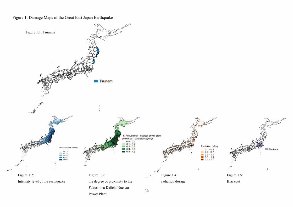
ignore other types of damage. Therefore, I construct 5 indices as the damage variables

regarding to tsunami, seismic intensity, proximity to the Fukushima Daiichi Plant,

radiation dose, and planned blackout. I define the indices as follows.

Tsunami - An indicator variable for the regions that suffered from the tsunami. This

variable takes on value 1 if the municipality is identified to have been submerged by the

tsunami and 0 otherwise (based on data from Saito et al., 2015).

Intensity4 - A continuous variable that measures the strength of the earthquake (in units

of Shindo) with the intensity level is 4 or more at each municipality. The seismic

intensity of the earthquake is constructed by the Japanese Meteorological Association

(hereafter JMA). As intensity is location specific, JMA has more than 1,700 observation

stations to measure earthquake intensity. Based on the Shindo scale, seismic intensity is

graded on 10 levels, beginning from 0 (“imperceptible to people”) and rising to 1, 2, 3,

4, 5-lower, 5-upper, 6-lower, 6-upper, and 7. At level 4, “most people are startled.”

I construct an intensity measure following Hanaoka et al. (2018). Specifically, the

measure is constructed using the weighted average of seismic intensities of the three

observation stations that are closest to a municipal office, with the weight being the

inverse of the distance between the municipal office and the respective observation

station. To capture the perceptional kink at level 4 of the Shindo scale, Hanaoka et al.

(2018) interact a continuous variable of intensity, �� , with an indicator

denoting that the intensity level is 4 or more, I[�� ≥ 4](�� − 4).

However, its identification may depend on the designed nonlinearity of the variable. To

avoid this concern, I mainly use I[�� ≥ 4](�� − 4) only for the

intensity variable, capturing the severity of the damages from earthquake intensity and

name this variable Intensity4.

Proximity - A continuous variable that indicates the degree of proximity to the

Fukushima Daiichi Nuclear Power Plant. Previous studies adopting a hedonic approach

often evaluated the damage arising from a nuclear accident by the distance from a

power station. For example, Gamble and Downing (1982) and Nelson (1981) estimated

the impact of the Three Mile Island nuclear power plant failure on the land prices of the

surrounding areas. These studies used the distance from the accident site as a proxy for

land damages.

7

Following the literature, I measure the distance between the Fukushima Daiichi Plant

and each municipal office and create an index of proximity to the Fukushima Daiichi

Plant. For consistency with other damage variables, the index is defined as the inverse

of distance (=100/distance in km), which takes a larger value if the magnitude of the

damage is assumed to be larger due to close proximity.

Radiation - A continuous variable that represents the radiation dosage in the

municipality. Radiation dosage is a standard means of evaluating the impact of a nuclear

accident and is widely used in the literature. For example, Kawaguchi and Yukutake

(2017) estimate the change in transaction prices before and after the Fukushima nuclear

accident with the degree of radioactive contamination. The radioactive contamination

degree captures similar but different variations as the proximity to the power plant since

it changes depending on wind directions.

I measure the radiation dosage for each municipality based on the aerial monitoring by

the Ministry of Education, Culture, Sports, Science and Technology. The measurement

of radiation dosage (units: µSv (microsieverts)) was taken by aircraft at altitudes of 150

to 300 m over the period from 22 June 2011 to 31 May 2012. I define the radiation

dosage of each municipality as the average dosage of the three survey points closest to

the municipal office and weighted by the inverse of the distance between them.

Blackout - An indicator variable for regions that were subject to scheduled blackout.

This variable takes the value 1 if the municipality was scheduled for blackout and 0

otherwise. Although there are few studies investigating the impact of blackouts, such

blackouts may have affected people’s fear and stress levels. For example, Burlando

(2014) reported that birth weights of children born 7–10 months after a month-long

power outage in Tanzania were lower.

To construct this variable, I depend on a “list of expected blackout areas” announced

by TEPCO on 15 March 2011. Despite being on the list, some municipalities were not

subjected to these blackouts. Since I am unable to obtain a list of these areas for

exclusion, I simply rely on TEPCO’s list.

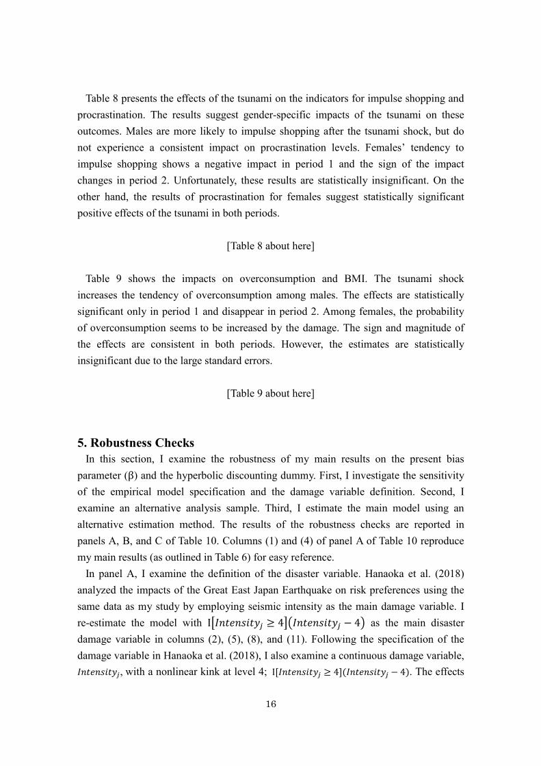
Table 1 summarizes the definitions and reports the summary statistics of each of the

damage indices. Figure 1 shows how the damages are distributed in Japan. A darker

color indicates a larger degree of damage. The damaged municipalities by tsunamis,

radiation, and blackouts are concentrated in relatively small areas. Although

municipalities that are somewhat damaged by the seismic intensity cover large areas,

8

limited regions are severely affected, i.e., have intensity levels greater than 4.

[Table 1 about here]

[Figure 1 about here]

2.3. Eliciting Time Preferences

2.3.1 Measures of Quasi-Hyperbolic Discounting

I use responses to the JHPS-CPS intertemporal trade-off questions to calculate each

individual’s quasi-hyperbolic discounting parameters, decomposing time preferences

into a present bias component β and a long-run component δ. The JHPS-CPS for

2011-2013 and 2016-2017 contain hypothetical questions with multiple price lists as

indicated below.

Question 1:

Suppose you are to receive money from someone. You can receive money today or 7

days later from today, but the amount will be different. Compare the amounts and dates

in option A and option B, and indicate which option you prefer for each of nine

combinations.

Question 2:

Suppose you are to receive money from someone. You can receive money 90 days later

or 97 days later from today, but the amount will be different. Compare the amounts and

dates in option A and option B, and indicate which option you prefer for each of nine

combinations.


The degree of time preference is measured by the row of the multi-price list where the

respondent changes her/his choice from option A to option B (i.e., combination of prices

of options A and B).１ Unfortunately, I cannot directly compare the values obtained

from each year’s survey responses. Despite the consistent wording of the questions, the

amounts quoted in the multi-price lists differ between the 2011 survey and the surveys

１Some respondents switched their choice between option A and option B more than once. Following

existing literature (e.g., Harrison et al., 2002), we treat their discount rates as missing values.

9

from 2012 onwards. The left panel of Table 2 shows how the amounts in the multi-price

lists differ in 2011 and in 2012 or later. I deal with this problem by regarding the range

of the multi-price list to be broader than it actually is. New group categories with

broader ranges are defined as indicated in the right panel of Table 2 with small letters

from a to g. For example, in the 2011 survey, respondents who switched their chosen

option from A to B at rows 2 and 3 are categorized into the same time discounting rate

level as those who switched options at rows 3 and 4.

I consider a model with quasi-hyperbolic discounting (Laibson, 1997; O’Donoghue

and Rabin, 1999) and exploit the two discount rates to compute a discount factor and a

present-bias. A time-consistent individual should have the same (annualized) discount

rate for “today or 7 days later” as “90 days or 97 days later.” In contrast, a

present-biased individual displays decreasing impatience and has a greater discount rate

for “today or 7 days later” than “90 days or 97 days later.” I jointly fit an individual’s

responses to both intertemporal questions using the quasi-hyperbolic discounting

specification (1).

�� = �(��) + β ∑ δ�� (��), (1)

where 0 ≤ δ ≤ 1 and 0 ≤ β ≤ 1.

The parameter δ (discount factor) reflects an individual’s long-run patience level

while β (present bias) reflects any disproportionate weight given to the immediate

present at the expense of all future periods. If β＝1, then the quasi-hyperbolic

discounting is the same as traditional, time-consistent discounting, whereas β < 1

reflects time-inconsistent present-bias. I also consider a discount function, &(⋅) such

that a utility, �, in τ -period is worth &(()� today.

Assuming annual periods, an individual’s responses to the two questions imply that

&��)�� *+�� (90 -+�� ). 97 -+�� 0+��.) = −0�1,

&��)�� *+�� (2)-+� ). 7 -+�� 0+��.) = −0�31. (2)

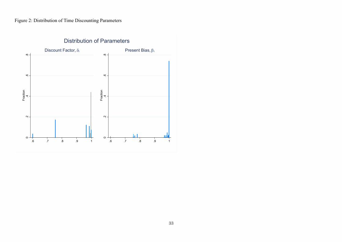
In the survey design of JHPS-CPS, the discount factor, δ, may have a value exceeding

1. Such a case is considered a corner solution and I let δ equal 1 as δ is between 0 and 1

by definition. Similarly, when β has a value more than 1, I let β equal 1.２ Figure 2

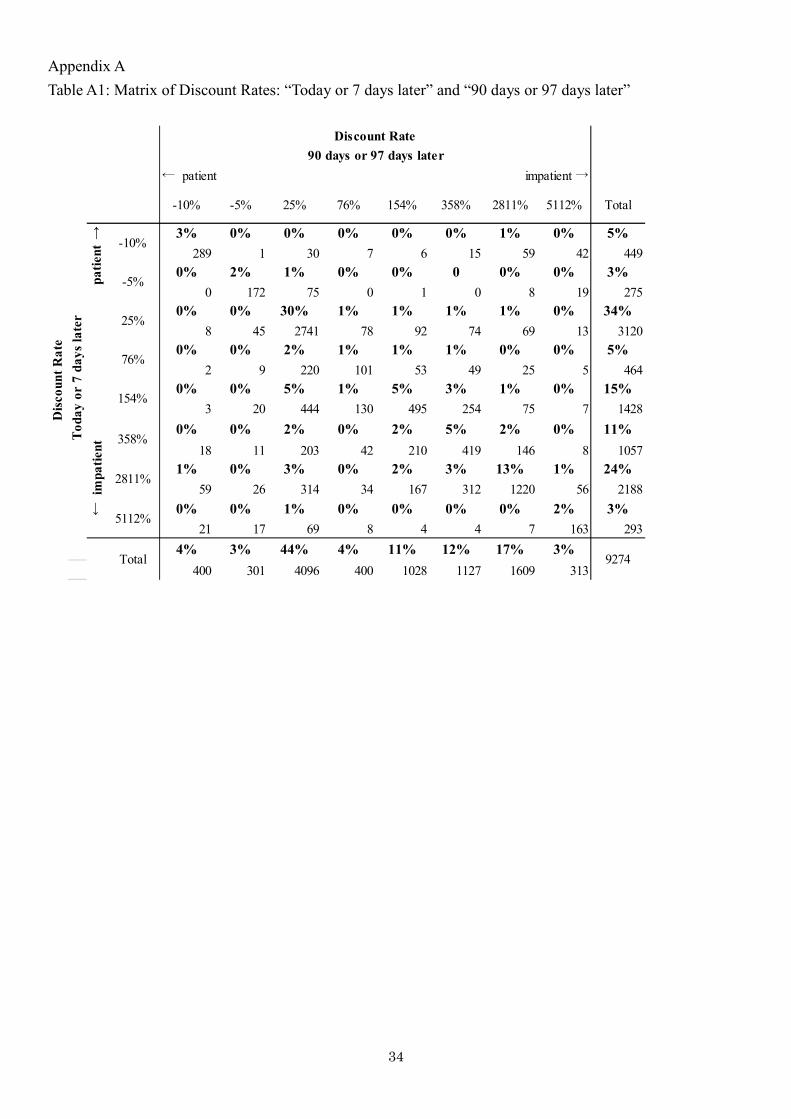
２The proportion of sample with discount factor, δ, is greater than 1 is 7.78%. The proportion of sample with present bias, β, is greater than 1 is 13.7%. See Table A1 (in Appendix) for more details, which shows the matrix of time discount rates of “today or 7 days later” and “90 days or 97 days later”. If the time discount rate “today or 7 days

10

shows the distribution of β and δ in pooled observations of total year. For δ, 7.6% of all

respondents have a time discount rate of 1. This means that the remaining 92.4%

respondents consider the future value to be discounted more than the current value. I

also construct a binary indicator of hyperbolic discounting which equals 1 if β < 1 and

0 otherwise. This indicator is more robust than β since it does not depend on the

method of determining the discount rate, and only indicates that the discount rates are

larger for “today or 7 days later” than for “90 days or 97 days later.”３ This indicator is

also robust to any hyperbolic discounting model other than the quasi-hyperbolic one.

One could argue that hypothetical questions, such as my intertemporal discounting

questions, provide no incentive for respondents to make decisions carefully, and thus the

estimated preferences based on such questions may not represent individuals’ true

preferences. Although some previous studies test a difference between hypothetical and

incentivized time discounting decisions, there is yet no consensus over the propriety of

the use of hypothetical questions in the literature. For example, Kirby and Maraković

(1995) found that subjects are more impatient when making a real decision than a

hypothetical one. Similarly, Coller and Williams (1999) noted that subjects are more

patient in the hypothetical decision. On the other hand, Johnson and Bickel (2002) and

Madden et al. (2003) found no difference in responses between real and hypothetical

time discounting decisions. I only assume that the bias is constant across all survey

years in the analysis. My empirical strategy considering the individual fixed effects

based on the panel data structure identifies the changes in preference. Therefore, the

results are robust up to a constant bias in hypothetical questions.

2.3.2 Alternative Proxies for Time Preferences

In addition to β and δ, I construct alternative proxy measures for time preferences.

Specifically, I create variables for impulse shopping, procrastination, BMI, and

overconsumption. First, I construct indicator variables for impulse shopping and

procrastination based on five-level categorical questions. In these questions,

respondents are asked how much a statement about a habitual behavior applies to them.

The specific statements are: “When I want something, I cannot help buying it” (impulse

shopping) and “If I have work that can wait to be done tomorrow, I wait until tomorrow

later” is less than the time discount rate “90 days or 97 days later”, the value of β is greater than 1. ３In this study, individuals’ time discounting rates are defined by the average value of discounting

rates before and after switching their chosen option in the multi-price lists. Their time discounting

rates may take any value within the range of the discount rate before and after the change in

selection, other than the average value.

11

to do it” (procrastination). The responses are based on a five-point scale with the

following categories: “This does not apply to me at all,” “This does not apply to me

very much,” “It is hard to say one way or the other,” “This applies to me somewhat,”

and “This applies to me perfectly.” I construct indicator variables that take the value 1 if

the respondent selects the option “This applies to me somewhat” or “This applies to me

perfectly,” and 0 otherwise. My hypothesis is that, ceteris paribus, if the respondents

become more impatient (smaller δ) or time-inconsistent (smaller β), they are more likely

to buy things impulsively, and if they become more time-inconsistent, they are more

likely to tend to procrastinate.

Second, I use respondents’ BMI defined as weight in kilograms divided by height in

meters squared (kg m7⁄ ). Courtemanche et al. (2015) and Ikeda et al. (2010) showed

that BMI is positively associated with impatience or time-inconsistent preferences. My

hypothesis is that, ceteris paribus, if respondents become more impatient (smaller δ) or

time-inconsistent (smaller β), they are more likely to have higher BMI than before.

Third, I construct an indicator variable to represent the relationship between actual

and planned changes in consumption. This variable takes value 1 if the respondent’s

actual increase in household consumption is larger than his/her scheduled increase in

consumption, and 0 otherwise. In the JHPS-CPS, there is a question regarding “How the

total expenditure of your household will change this year compared with the previous

year.” In the same year’s survey, there is a question that asks “how last year’s total

household expenditure of respondents’ changed compared with two years ago.”４

By comparing the actual consumption change reported in a survey year and the

planned consumption change based on the previous year’s survey, I can determine

whether respondents have over-consumed beyond their original plan. This variable is

unavailable for 2013 and 2017 due to the missing surveys in the next consecutive year.５

４This question is asked every year. For example, the 2013 survey (conducted in February), asked:

Q1. How is the total expenditure of your household expected to change in 2013 compared with

2012?

Q2. How has the total expenditure of your household changed in 2012 compared with 2011?

1. Increased by at least 9%”

2. Increased by at least 7% but less than 9%




6. Changed by less than 1% in either direction

7. Decreased by at least 1% but less than 3%




11. Decreased by at least 9% ５For example, the question about actual consumption change from 2011 to 2012 that is asked in the

12

In addition, it is natural for people living in damaged areas to actually over-consume in

2011 compared to their planned consumption reported before the earthquake. Therefore,

I drop the 2011 data from my estimation.

Table 3 presents the summary statistics of individuals’ time preferences and

characteristics. The analysis data includes only those respondents who answered all

surveys from 2009 to 2017. However, the data are an unbalanced panel structure

because some respondents, occasionally, do not answer basic questions about their

characteristics in a survey year. Since the survey is conducted every February, surveys

in 2009-2011 were conducted before the Great East Japan Earthquake (March 11, 2011).

Therefore, I can observe individuals' change both immediately after (in 2012 and 2013,

hereafter After_Term1) and several years after the earthquake (in 2016 and 2017,

hereafter After_Term2) in the analysis data.


Table 4 shows the t-test results, comparing the means of the time preference variables

between respondents affected and unaffected by the earthquake, based on the survey

conducted before the earthquake. I find a statistically significant difference in

pre-earthquake hyperbolic discounting probability. This indicates that if I had only the

data after the earthquake, I would incorrectly recognize the difference in preferences

between those affected and unaffected it had been since before the disaster as the effect

of the earthquake.


2.4 Selective Attrition

The selective attrition of particular types of individuals can bias my estimates. If

people who are more adversely affected by the earthquake are more likely to migrate in

its aftermath and not respond to the survey, my analysis would only capture the changes

in preferences of peculiar remaining residents. Since the 2012 survey, the JHPS-CPS

has initiated follow-up surveys with people who have migrated. The migration rates are

fairly low at less than 1 percent. This is so because respondents whose municipality

2013 survey can be used to compute the overconsumption in 2012 compared to the scheduled

change reported in the 2012 survey. However, I cannot ascertain how the scheduled consumption in

2013 was changed in 2014 since the survey was not implemented in 2014.

13

differs between two years are counted as cases of attrition and not migration. Therefore,

I need to consider the effect of sample attrition.

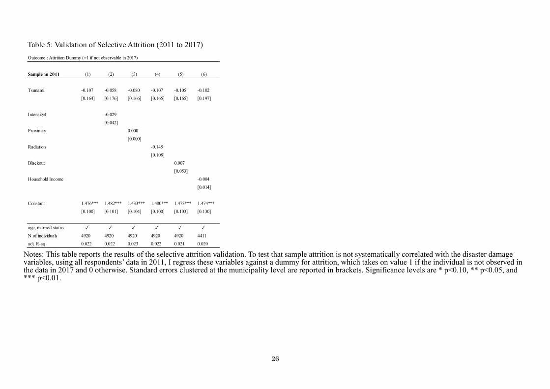
Given the availability of data before the earthquake, I can check whether the attritions

are selective or not. To test that sample attrition is orthogonal to the disaster damage

variables, using data of all respondents in 2011, I regress these variables against a

dummy for attrition, which takes on value 1 if the individual is not observed after the

earthquake and 0 otherwise. Table 5 shows that the attrition is not systematically

correlated with the disaster damage variables. This suggests that there is no evidence of

selective attrition after the earthquake in my analyzed data.


3. Identification Strategy

I examine the effects of the earthquake on time preferences using panel data before

and after its occurrence. Employing a difference-in-difference model, I control for

time-invariant individual characteristics using individual fixed effects. I capture the

change in time preferences by comparing a sample of individuals affected by the

earthquake (the treatment group) versus others who remain unaffected (the control

group). The following baseline model is used to estimate the earthquake impacts:

2�9� :.�;�.��<�� = α>

+3 2��+9�� + γ�2��+9�� ∗ A;��._2�.91 + γ72��+9�� ∗ A;��._2�.92

+θ�A;��._2�.91 + θ7A;��._2�.92 + πF<�� + G<��.

(3)

where 2�9� :.�;�.��<�� is a variable of time preferences for individual i at

location j at time t and H< represents time-invariant individual characteristics.

2��+9�� is an indicator variable for suffered from the tsunami at location j. The

coefficient β of 2��+9�� is not identified because the time-invariant individual

fixed effects are also controlled in the model; therefore, this term is omitted in the

estimation. After_Term1is a dummy variable that takes the value 1 if the year is in

period 1: 2012 or 2013 survey years, and 0 otherwise. A;��._��.92 is a dummy

variable that takes the value 1 if the year is in period 2: 2016 or 2017, and 0 otherwise.

The coefficients of the interactions of these dummies and 2��+9�� are parameters of

interest. More specifically, γ� represents the changes in preferences immediately after

the disaster, and γ7 represents the changes in preferences after a lag following the

disaster. θ� and θ7 indicate the time effects on outcomes at each respective period. I

14

do not use the year dummy variable for each year but two-period dummies after the

earthquake because the number of individuals adversely affected by the tsunami is small.

I also control age, marriage status as time-variant individual characteristics (F<��). G<��

is the idiosyncratic random shock.

One concern is that the estimates representing the change caused by the tsunami may

include changes caused by the other damages, such as large shaking and the nuclear

accident. To mitigate this concern, in the model (4), I add the other damage variables to

the baseline model (3).

2�9� :.�;�.��<�� = α>

+32��+9�� + γ�2��+9�� ∗ A;��._2�.91 + γ72��+9�� ∗ A;��._2�.92

+I&+9+J�� + μ�&+9+J�� ∗ A;��._2�.91 + μ7&+9+J�� ∗ A;��._2�.92

+θ�A;��._2�.91 + θ7A;��._2�.92 + πF<�� + G<��,

(4)

where &+9+J�� represents a disaster damage variable other than tsunami at

location j.

I also employ a model controlling household income variable to clarify the

mechanism of preference change. As Hauster and Fehr (2014) suggests, poverty can

affect the individuals’ time preferences. When the preferences of those injured by the

disaster are changed due to the poverty, adding household income as a control variable

should eliminate the peculiar change in the disaster area (γ� +�- γ7).

4. Results

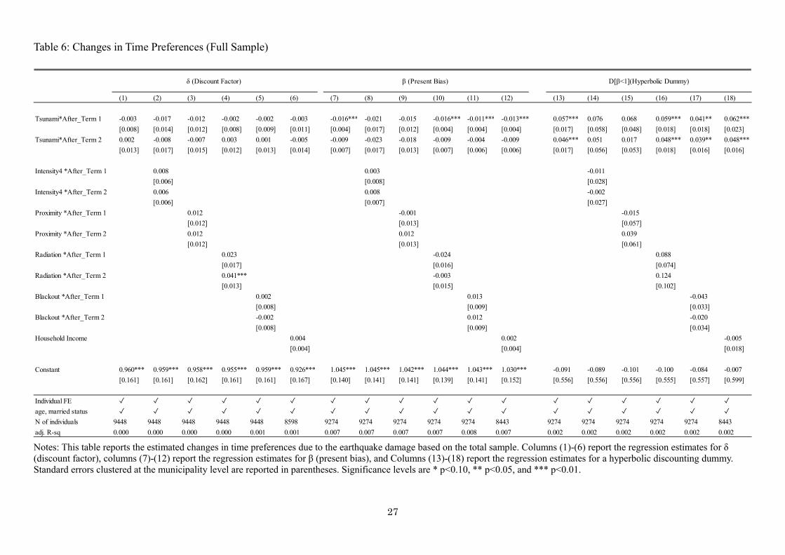
4.1 Changes in β, δ, and Hyperbolic Discounting

Table 6 illustrates how the earthquake damage changes δ (discount factor), β (present

bias), and the hyperbolic discounting dummy variable. I mainly focus on the effects of

the tsunami variable and include the other damage variables to examine the robustness

of the results.

I begin with a simple regression of time preferences on the interaction of tsunami and

after-dummies in column (1), and add interaction terms for the other disaster damage

variables or household income to the baseline model. The columns from (1) to (6) show

that the tsunami does not bring statistically significant change to the discount factor (δ).

The magnitudes of the effects are very small, and the signs are unstable over the two

periods and for the other disaster damage variable controls.

Columns from (7) to (12) show the statistically significant negative effects of the

15

tsunami on present bias (β) in After_Term1 except for the regression results in columns

(8) and (9). However, the effects remain negative but statistically insignificant in

After_Term2. This implies that the present bias increased immediately after the

earthquake and has since reverted to the original, pre-earthquake level. The results also

suggest the importance of differentiating the present bias from the discount factor.

Columns from (13) to (18) report the effects on the probability of hyperbolic

discounting. The tsunami significantly increases the hyperbolic probability over the

periods under study, and the magnitudes of the effects are reasonably large not only in

After_Term1 but also in After_Term2. The results are robust in terms of controlling the

other damage variables except for columns (14) and (15). These findings suggest that

time preferences are significantly affected by the tsunami after the earthquake and that

the change persists in the long-term. These significant changes in present bias are robust

to controlling for the household income in columns (12) and (18). This suggests that the

changes in present bias are not caused by poverty.


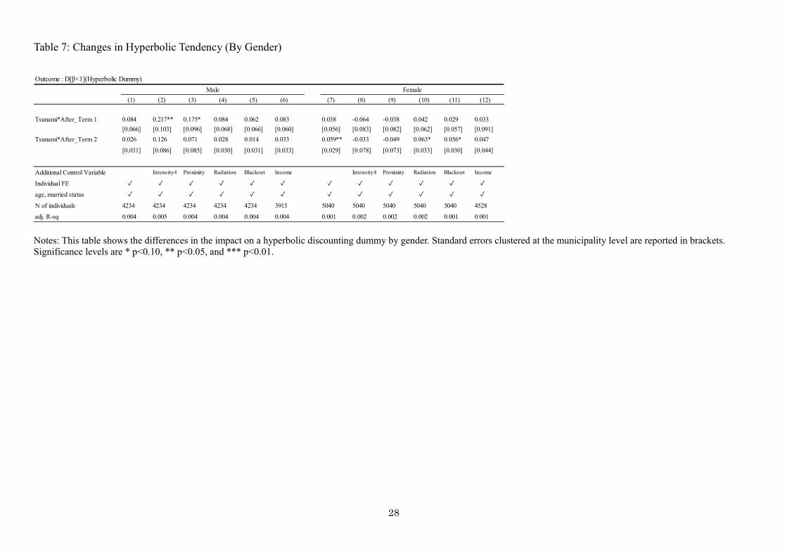
In Table 7, I investigate whether the effects of the tsunami on hyperbolic discounting

are heterogeneous by gender I divide the sample by gender and re-estimate the models

in columns (13) to (19) of Table 6. The results suggest that the tsunami increases

hyperbolic discounting probability among males, and the effects are statistically

significant in columns (2) and (3) in A;��._2�.9�. The effects on females are in the

same direction as that of males except for columns (8) and (9), but are statistically

significant in A;��._2�.97. (columns (7), (10), and (11)). These findings suggest that

changes in time preferences are immediate and temporary for males, but appear after a

few years for females.


4.2 Changes in Actual Behavior

The main results outlined in Tables 6 and 7 suggest that time preferences are

significantly changed by the damage caused by the earthquake. One consideration is

whether these changes are actual changes in preferences and whether they would bring

about changes in actual behavior after the earthquake. To examine this concern, I

estimate the model using actual behavior variables as the dependent variable.

16

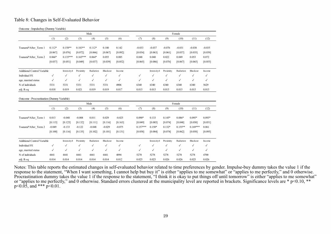
Table 8 presents the effects of the tsunami on the indicators for impulse shopping and

procrastination. The results suggest gender-specific impacts of the tsunami on these

outcomes. Males are more likely to impulse shopping after the tsunami shock, but do

not experience a consistent impact on procrastination levels. Females’ tendency to

impulse shopping shows a negative impact in period 1 and the sign of the impact

changes in period 2. Unfortunately, these results are statistically insignificant. On the

other hand, the results of procrastination for females suggest statistically significant

positive effects of the tsunami in both periods.


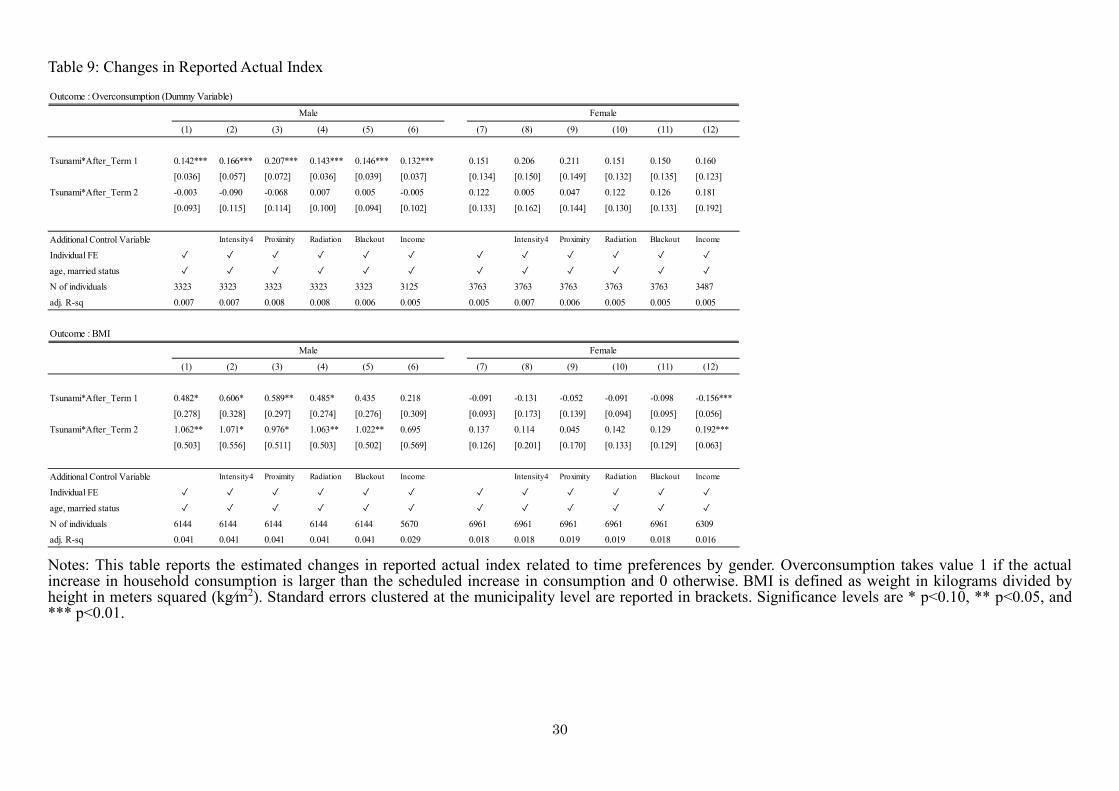
Table 9 shows the impacts on overconsumption and BMI. The tsunami shock

increases the tendency of overconsumption among males. The effects are statistically

significant only in period 1 and disappear in period 2. Among females, the probability

of overconsumption seems to be increased by the damage. The sign and magnitude of

the effects are consistent in both periods. However, the estimates are statistically

insignificant due to the large standard errors.


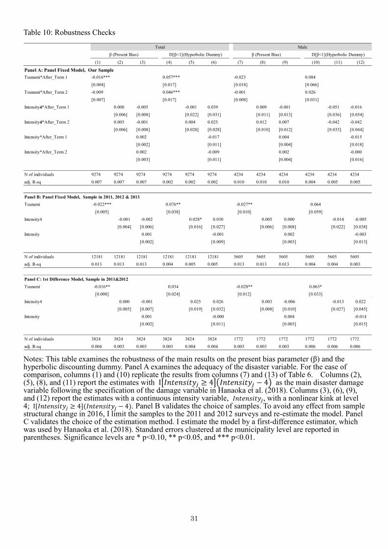
5. Robustness Checks

In this section, I examine the robustness of my main results on the present bias

parameter (β) and the hyperbolic discounting dummy. First, I investigate the sensitivity

of the empirical model specification and the damage variable definition. Second, I

examine an alternative analysis sample. Third, I estimate the main model using an

alternative estimation method. The results of the robustness checks are reported in

panels A, B, and C of Table 10. Columns (1) and (4) of panel A of Table 10 reproduce

my main results (as outlined in Table 6) for easy reference.

In panel A, I examine the definition of the disaster variable. Hanaoka et al. (2018)

analyzed the impacts of the Great East Japan Earthquake on risk preferences using the

same data as my study by employing seismic intensity as the main damage variable. I

re-estimate the model with IL�� ≥ 4MN�� − 4O as the main disaster

damage variable in columns (2), (5), (8), and (11). Following the specification of the

damage variable in Hanaoka et al. (2018), I also examine a continuous damage variable,

��, with a nonlinear kink at level 4; I[�� ≥ 4](�� − 4). The effects

17

of the intensity on β and the hyperbolic dummy are very small or negligible compared

to the significant negative effects of the tsunami.

The estimates in panel B validate the choice of samples. An important concern of the

JHPS-CPS is that it was once suspended and has resumed since 2016 with a portion of

the original respondents of the 2013 survey. To avoid any effect from this sample

structural change, I limit the samples to the 2011 and 2012 surveys and re-estimate the

model. The results show that my main finding of a statistically significant effect of the

tsunami on β and the Hyperbolic dummy are robust to the choice of samples. There is

also a statistically significant impact of intensity on the hyperbolic dummy in column

(5) only. However, it is not robust and is supposed to reflect the effect of the tsunami.

In panel C, I mainly focus on the estimation method. In addition to the specification

and the sample choice checks in panels A and B, I estimate the model by a

first-difference estimator, which was used by Hanaoka et al. (2018). In contrast, I have

used a fixed-effect estimator in the main analysis. The results are virtually unchanged

by the different estimation method.


6. Conclusion

I investigated whether individuals’ time preferences are changed by the damage

caused by the tsunami in the Great East Japan Earthquake of 2011, using panel surveys

before and after the earthquake. I find that the change in time discount rate (δ) is not

statistically significant for those who are adversely impacted by the tsunami, although

the present bias tendency is increased (shrinking β) significantly. I also find that those

adversely affected by the tsunami are more prone to make impulse shopping,

procrastinate, over-consume, and increase their BMI. Changes in time preferences

appeared in males immediately after the earthquake in 2012 and 2013, and are subsiding

ever since. On the other hand, in the case of females, these changes appeared in 2016

and 2017, after a lag since the earthquake.

The findings suggest that changes in present bias tendency for those affected by a

disaster are an important factor in the post-disaster reconstruction process, and might

partly explain differences between immediate and delayed reconstruction performances

after disasters all over the world. However, I am unable to clarify why and how the time

preference was affected by the disaster in detail due to the data limitation. I also

18

acknowledge that a gender difference in the changes is not fully understood in the

present study. These questions are beyond the scope of my study and are left for the

future research.

19

References

Burks, S., Carpenter, J., Götte, L., Rustichini, A., 2012. Which measures of time

preference best predict outcomes: Evidence from a large-scale field experiment.

Journal of Economic Behavior & Organization 84(1), 308–320. DOI:

https://doi.org/10.1016/j.jebo.2012.03.012

Burlando, A., 2014. Transitory shocks and birth weights: Evidence from a blackout in

Zanzibar. Journal of Development Economics 108, 154–168. DOI:

https://doi.org/10.1016/j.jdeveco.2014.01.012

Callen, M., 2015. Catastrophes and time preference: Evidence from the Indian Ocean

Earthquake. Journal of Economic Behavior & Organization 118, 199–214. DOI:


Cameron, L., Shah, M., 2015. Risk-taking behavior in the wake of natural disasters.

Journal of Human Resources 50(2), 484–515. DOI:

https://doi.org/10.3368/jhr.50.2.484

Chuang, Y., Schechter, L., 2015. Stability of experimental and survey measures of risk,

time, and social preferences: A review and some new results. Journal of

Development Economics 117, 151–170. DOI:

https://doi.org/10.1016/j.jdeveco.2015.07.008

Coller, M., Williams, M.B., 1999. Eliciting individual discount rates. Experimental

Economics 2(2), 107–127. DOI: https://doi.org/10.1007/BF01673482

Courtemanche, C., Heutel, G., McAlvanah, P., 2015. Impatience, incentives, and obesity.

The Economic Journal 125(582), 1–31. DOI: https://doi.org/10.1111/ecoj.12124

Eckel, C.C., El-Gamal, M.A., Wilson, R.K., 2009. Risk loving after the storm: A

Bayesian-Network study of Hurricane Katrina evacuees. Journal of Economic

Behavior & Organization 69(2), 110–124. DOI:


Fields, S.A., Lange, K., Ramos, A., Thamotharan, S, Rassu, F., 2014. The relationship

between stress and delay discounting: A meta-analytic review. Behavioural

Pharmacology, 25(5 and 6), 434–444. DOI:

https://doi:10.1097/FBP.0000000000000044

Frederick, S., Loewenstein, G., O’Donoghue, T., 2002. Time discounting and time

preference: A critical review. Journal of Economic Literature 40(2), 351–401.

DOI: https://doi.org/10.1257/002205102320161311

Gamble, H.B., Downing, R.H., 1982. Effects of nuclear power plants on residential

property values. Journal of Regional Science 22(4), 457–478. DOI:

20

https://doi.org/10.1111/j.1467-9787.1982.tb00770.x

Hanaoka, C., Shigeoka, H., Watanabe, Y. 2018. Do risk preferences change? Evidence

from the Great East Japan Earthquake. American Economic Journal: Applied

Economics 10(2), 298–330. DOI: https://doi.org/10.1257/app.20170048

Harrison, G.W., Lau, M.I., Williams, M.B., 2002. Estimating individual discount rates

in Denmark: A field experiment. American Economic Review 92(5), 1606–1617.

DOI: https://doi.org/10.1257/000282802762024674

Ikeda, S., Kang, M.I., Ohtake, F., 2010. Hyperbolic discounting, the sign effect, and the

body mass index. Journal of Health Economics 29(2), 268–284. DOI:

https://doi.org/10.1016/j.jhealeco.2010.01.002

Johnson, M.W., Bickel, W.K., 2002. Within-subject comparison of real and hypothetical

money rewards in delay discounting. Journal of the Experimental Analysis of

Behavior 77(2), 129–146. DOI: https://doi.org/10.1901/jeab.2002.77-129

Kawaguchi, D., Yukutake, N., 2017. Estimating the residential land damage of the

Fukushima nuclear accident. Journal of Urban Economics 99, 148–160. DOI:

https://doi.org/10.1016/j.jue.2017.02.005

Kirby, K.N., Maraković, N.N., 1995. Modeling myopic decisions: Evidence for

hyperbolic delay-discounting within subjects and amounts. Organizational

Behavior and Human Decision Processes 64(1), 22–30. DOI:

https://doi.org/10.1006/obhd.1995.1086

Laibson, D.I., 1996. Hyperbolic discount functions, undersaving, and savings policy.

National Bureau of Economic Research, NBER Working Paper No. 5635. DOI:

https://doi.org/10.3386/w5635

Laibson, D.I., 1997. Golden eggs and hyperbolic discounting. The Quarterly Journal of

Economics 112(2), 443–478. DOI: https://doi.org/10.1162/003355397555253

Madden, G. J., Begotka, A. M., Raiff, B. R., Kastern, L. L. 2003. Delay discounting of

real and hypothetical rewards. Experimental and Clinical Psychopharmacology,

11(2), 139–145. DOI: http://doi.org/10.1037/1064-1297.11.2.139

Nelson, J.P., 1981. Three Mile Island and residential property values: Empirical analysis

and policy implications. Land Economics 57(3), 363–372. DOI:

https://doi.org/10.2307/3146017

O’Donoghue, T., Rabin, M., 1999. Doing it now or later. American Economic Review

89(1), 103–124. DOI: https://doi.org/10.1257/aer.89.1.103

Rehdanz, K., Welsch, H., Narita, D., Okubo, T., 2015. Well-being effects of a major

natural disaster: The case of Fukushima. Journal of Economic Behavior &

Organization 116, 500–517. DOI: https://doi.org/10.1016/j.jebo.2015.05.014

21

Saito, M., Nakagawa, M., Gu, T. 2015. How was the recovery budget for the Great East

Japan Earthquake created? In M. Saito (Ed.), Earthquake and Economics, 1—32.

TOYO KEIZAI INC.

The National Police Agency 2012. The Great East Japan Earthquake and police, Focus

No. 281. Available from:

https://www.npa.go.jp/archive/keibi/syouten/syouten281/pdf/ALL.pdf (in

Japanese)

Tokyo Electric Power Company (TEPCO), 2011. List of expected blackout areas (online

cited 9 January 2013).

Yamamura, E., Tsutsui, Y., Yamane, C., Yamane, S., Powdthavee, N., 2015. Trust and

happiness: Comparative study before and after the Great East Japan Earthquake.

Social Indicators Research 123(3), 919–935. DOI:

https://doi.org/10.1007/s11205-014-0767-7

22

Table 1: Summary Statistics of Damage Variables at the Municipality Level

Notes: This table reports summary statistics of the damage variables. These five damage variables are constructed at the municipality level based on respondents’ residential information as at the 2011 survey.

Mean

[S.D.]

Tsunami A binary indicator for tsunami damage regions, which takes on value 1 140 0.02 0 1

if the region is affected by the tsunami and 0 otherwise. [0.15]

Intensity4 A continuous variable that measures the strength of the earthquake 140 0.40 0.00 2.33

with the intensity level is 4 or more, I[Intensity≥4}(Intensity-4). [0.62]

Proximity Proximity of Fukushima Daiichi Nuclear Power Station to the region 140 483.42 56.92 1,769.24

,100 / distance (km). [331.89]

Radiation Radiation dosage (unit: μSv) 140 0.05 0.00 1.02

[0.15]

Blackout A binary indicator for scheduled blackout which equals 1 140 0.28 0 1

if the region was subject to scheduled blackouts and 0 otherwise. [0.45]

Variables Definition Obs. Min Max

23

Table 2: Questions to Elicit Discount Rates

Notes: The amounts in the multi-price lists differ between the 2011 survey and the surveys conducted from 2012 onwards. The left panel of Table 2 reflects these differences while the right panel illustrates how I deal with this problem, i.e., by regrouping the multi-price list into broader categories than the original.

in 2011

Group Annual Interest Group Discount Rate

in survey Rate (approx). in this paper in survey in this paper in this paper

1 JPY 3,006 (USD 26.20) JPY 3,000 (USD 26.14) -10% a -10%

2 JPY 3,001 (USD 26.15) JPY 3,001 (USD 26.15) 0% b 1/2 a/b -5%

3 JPY 3,002 (USD 26.16) JPY 3,008 (USD 26.21) 10% 2/3

4 JPY 3,000 (USD 26.14) JPY 3,029 (USD 26.40) 50% 3/4

5 JPY 3,006 (USD 26.20) JPY 3,065 (USD 26.71) 102% d 4/5 c/d 76%

6 JPY 3,007 (USD 26.20) JPY 3,125 (USD 27.23) 205% e 5/6 d/e 154%

7 JPY 3,000 (USD 26.14) JPY 3,176 (USD 27.68) 306% 6/7

8 JPY 3,007 (USD 26.20) JPY 3,302 (USD 28.78) 512% 7/8

9 JPY 3,007 (USD 26.20) JPY 5,955 (USD 51.90) 5112% g 8/9 f/g 2811%

5112%

in 2012 or later

Group Annual Interest group Discount Rate

in survey Rate (approx). in this paper in survey in this paper in this paper

1 JPY 3002 (USD 26.20) JPY 2996 (USD 26.14) -10% a choose Option A for all choices -10%

2 JPY 3000 (USD 26.15) JPY 3000 (USD 26.15) 0% b 1/2 a/b -5%

3 JPY 3008 (USD 26.19) JPY 3011 (USD 26.19) 5% 2/3

4 JPY 3005 (USD 26.14) JPY 3014 (USD 26.22) 16% 3/4

5 JPY 3008 (USD 26.20) JPY 3037 (USD 26.45) 50% 4/5

6 JPY 3009 (USD 26.20) JPY 3068 (USD 26.72) 102% d 5/6 c/d 76%

7 JPY 3001 (USD 26.14) JPY 3119 (USD 27.17) 205% e 6/7 d/e 154%

8 JPY 3003 (USD 26.20) JPY 3297 (USD 28.77) 510% f 7/8 e/f 358%

9 JPY 3005 (USD 26.20) JPY 5951 (USD 51.90) 5112% g 8/9 f/g 2811%

5112%

Calculation of Time Discount Rates

Choose Option A for all choices

b/c

e/f

Switch from A to B at

Questionnaire

Option A

Receipt today (90 days later) Receipt 7 days later (97 days later)

Option B

f

c

25%

Switch from A to B at

choose Option B for all choices

c b/c


Option A Option B

Calculation of Time Discount RatesQuestionnaire

Choose Option B for all choices

25%

358%

24

Table 3: Summary Statistics of Variables Representing Individuals’ Time Preferences & Characteristics

Notes: This table reports the summary statistics of the variables used in the analysis for each year. “n/a” indicates that the question was not asked in the year since the JHPS-CPS does not ask exactly the same questions each year. Standard deviations are in parentheses.

Obs. Mean Obs. Mean Obs. Mean Obs. Mean Obs. Mean Obs. Mean Obs. Mean

(S.D.) (S.D.) (S.D.) (S.D.) (S.D.) (S.D.) (S.D.)

Time Preferences

δ (Discount Factor) Time discount factor, which is computed based on 0 n/a 0 n/a 1,888 0.94 1,881 0.94 1,890 0.93 1,894 0.94 1,895 0.94

choice of 90 days or 97 days later in Table 1. (0.11) (0.11) (0.11) (0.11) (0.11)

β (Present Bias) The present bias, which is computed based on Table 1, 0 n/a 0 n/a 1,820 0.96 1,858 0.97 1,865 0.97 1,861 0.97 1,870 0.97

comparing choice of today or 7-days later to that of 90 days or 97 days later. (0.10) (0.08) (0.08) (0.08) (0.07)

D[β<1](Hyperbolic Dummy) A binary indicator for hyperbolic discounting, which equals 1 0 n/a 0 n/a 1,820 0.76 1,858 0.79 1,865 0.79 1,861 0.79 1,870 0.79

if Beta<1 and 0 otherwise. (0.43) (0.41) (0.41) (0.41) (0.40)

Self-evaluated Behavior Relating to Time Preference

Impulse shopping A binary indicator for an impulse shopping which equals 1 if the response 1,955 0.24 1,945 0.25 0 n/a 1,931 0.17 1,945 0.16 1,946 0.18 1,949 0.17

to the statement "When I want something, I cannot help but buy it" is either (0.43) (0.43) (0.38) (0.37) (0.38) (0.38)

"apply me somewhat" or "apply me perfectly", and 0 otherwise.

Procrastination A binary indicator for a procrastination which equals 1 if the response 1,953 0.59 0 n/a 0 n/a 1,930 0.46 1,944 0.47 1,948 0.48 1,944 0.46

to the statement "I think it's okey to put things off until tomorrow" is either (0.49) (0.50) (0.50) (0.50) (0.50)

"apply me somewhat" or "apply me perfectly", and 0 otherwise.

Reported Actual Index Relating to Time Preference

BMI Body mass index (kg/(m 2̂)) 1,866 22.632 1,870 22.65 1,886 22.70 1,884 22.72 1,878 22.78 1,874 22.79 1,847 22.79

(3.29) (3.17) (3.23) (3.17) (3.26) (3.32) (3.31)

Overconsumption A binary indicator for overspending, which equals 1 if 1,732 0.40 1,757 0.45 0 n/a 1,777 0.38 0 n/a 1,820 0.37 0 n/a

actual consumption > scheduled consumption and 0 otherwise. (0.49) (0.50) (0.48) (0.48)

Individual Characteristics

Male A binary indicator for gender, which equals 1 if the respondent 1,957 0.46 1,951 0.46 1,952 0.46 1,949 0.46 1,949 0.46 1,952 0.46 1,952 0.46

is male and 0 otherwise (0.50) (0.50) (0.50) (0.50) (0.50) (0.50) (0.50)

Age Age of respondent 1,957 49.90 1,951 50.91 1,952 51.91 1,949 52.93 1,949 53.94 1,952 56.88 1,952 57.89

(11.76) (11.75) (11.75) (11.74) (11.73) (11.75) (11.75)

Married A binary indicator for marriage status which equals 1 if married, 1,957 0.82 1,951 0.82 1,952 0.82 1,949 0.82 1,949 0.81 1,952 0.80 1,952 0.80

and 0 otherwise. (0.38) (0.38) (0.38) (0.39) (0.39) (0.40) (0.40)

Income Log of per capita household income in million yen. 1,732 2.77 1,738 2.76 1,762 2.74 1,761 2.73 1,758 2.72 1,796 2.72 1,783 2.72

(0.56) (0.56) (0.55) (0.56) (0.55) (0.54) (0.57)

Before Earthquake After_Term1 After_Term2

2017

Variable Definition

2009 2010 2011 2012 2013 2016

25

Table 4: t-Test of Time preferences for Affected and Unaffected Individuals

Notes: This table reports group means of affected and unaffected individuals with corresponding deviations in parentheses. The point estimate shows the mean difference of time preferences before the earthquake between individuals who were affected and those unaffected by the tsunami with corresponding standard errors in brackets. Data are based on the survey of the most recent (single) year before the earthquake occurred.

Unaffected Affected p-Value

Mean Mean Difference

Year (S.D.) (S.D.) [S.E.]

Time Preferences

δ (Discount Factor) in 2011 0.937 0.930 0.007 0.707

(0.114) (0.123) [0.018]

β (Present Bias) in 2011 0.958 0.968 -0.010 0.493

(0.098) (0.089) [0.015]

D[β<1](Hyperbolic Dummy) in 2011 0.291 0.167 0.124 0.079

(0.454) (0.089) [0.071]

Self-evaluation Behavior Relating to Time Preference

Impulse Shopping in 2010 0.247 0.180 0.067 0.278

(0.431) (0.388) [0.062]

Procrastination in 2009 0.594 0.540 0.054 0.445

(0.491) (0.503) [0.070]

Reported Actual Index Relating to Time Preference

BMI in 2011 22.698 22.891 -0.193 0.678

(3.239) (3.108) [0.464]

Overconsumption in 2011 0.446 0.550 -0.104 0.192

(0.497) (0.504) [0.080]

HQ: Unaffected= Affected

26

Table 5: Validation of Selective Attrition (2011 to 2017)

Notes: This table reports the results of the selective attrition validation. To test that sample attrition is not systematically correlated with the disaster damage variables, using all respondents’ data in 2011, I regress these variables against a dummy for attrition, which takes on value 1 if the individual is not observed in the data in 2017 and 0 otherwise. Standard errors clustered at the municipality level are reported in brackets. Significance levels are * p<0.10, ** p<0.05, and *** p<0.01.

Outcome : Attrition Dummy (=1 if not observable in 2017)

Sample in 2011 (1) (2) (3) (4) (5) (6)

Tsunami -0.107 -0.058 -0.080 -0.107 -0.105 -0.102

[0.164] [0.176] [0.166] [0.165] [0.165] [0.197]

Intensity4 -0.029

[0.042]

Proximity 0.000

[0.000]

Radiation -0.145

[0.108]

Blackout 0.007

[0.053]

Household Income -0.004

[0.014]

Constant 1.476*** 1.482*** 1.433*** 1.480*** 1.473*** 1.474***

[0.100] [0.101] [0.104] [0.100] [0.103] [0.130]

age, married status ✓ ✓ ✓ ✓ ✓ ✓

N of individuals 4920 4920 4920 4920 4920 4411

adj. R-sq 0.022 0.022 0.023 0.022 0.021 0.020

27

Table 6: Changes in Time Preferences (Full Sample)

Notes: This table reports the estimated changes in time preferences due to the earthquake damage based on the total sample. Columns (1)-(6) report the regression estimates for δ

(discount factor), columns (7)-(12) report the regression estimates for β (present bias), and Columns (13)-(18) report the regression estimates for a hyperbolic discounting dummy.

Standard errors clustered at the municipality level are reported in parentheses. Significance levels are * p<0.10, ** p<0.05, and *** p<0.01.

(1) (2) (3) (4) (5) (6) (7) (8) (9) (10) (11) (12) (13) (14) (15) (16) (17) (18)

Tsunami*After_Term 1 -0.003 -0.017 -0.012 -0.002 -0.002 -0.003 -0.016*** -0.021 -0.015 -0.016*** -0.011*** -0.013*** 0.057*** 0.076 0.068 0.059*** 0.041** 0.062***

[0.008] [0.014] [0.012] [0.008] [0.009] [0.011] [0.004] [0.017] [0.012] [0.004] [0.004] [0.004] [0.017] [0.058] [0.048] [0.018] [0.018] [0.023]

Tsunami*After_Term 2 0.002 -0.008 -0.007 0.003 0.001 -0.005 -0.009 -0.023 -0.018 -0.009 -0.004 -0.009 0.046*** 0.051 0.017 0.048*** 0.039** 0.048***

[0.013] [0.017] [0.015] [0.012] [0.013] [0.014] [0.007] [0.017] [0.013] [0.007] [0.006] [0.006] [0.017] [0.056] [0.053] [0.018] [0.016] [0.016]

Intensity4 *After_Term 1 0.008 0.003 -0.011

[0.006] [0.008] [0.028]

Intensity4 *After_Term 2 0.006 0.008 -0.002

[0.006] [0.007] [0.027]

Proximity *After_Term 1 0.012 -0.001 -0.015

[0.012] [0.013] [0.057]

Proximity *After_Term 2 0.012 0.012 0.039

[0.012] [0.013] [0.061]

Radiation *After_Term 1 0.023 -0.024 0.088

[0.017] [0.016] [0.074]

Radiation *After_Term 2 0.041*** -0.003 0.124

[0.013] [0.015] [0.102]

Blackout *After_Term 1 0.002 0.013 -0.043

[0.008] [0.009] [0.033]

Blackout *After_Term 2 -0.002 0.012 -0.020

[0.008] [0.009] [0.034]

Household Income 0.004 0.002 -0.005

[0.004] [0.004] [0.018]

Constant 0.960*** 0.959*** 0.958*** 0.955*** 0.959*** 0.926*** 1.045*** 1.045*** 1.042*** 1.044*** 1.043*** 1.030*** -0.091 -0.089 -0.101 -0.100 -0.084 -0.007

[0.161] [0.161] [0.162] [0.161] [0.161] [0.167] [0.140] [0.141] [0.141] [0.139] [0.141] [0.152] [0.556] [0.556] [0.556] [0.555] [0.557] [0.599]

Individual FE ✓ ✓ ✓ ✓ ✓ ✓ ✓ ✓ ✓ ✓ ✓ ✓ ✓ ✓ ✓ ✓ ✓ ✓

age, married status ✓ ✓ ✓ ✓ ✓ ✓ ✓ ✓ ✓ ✓ ✓ ✓ ✓ ✓ ✓ ✓ ✓ ✓

N of individuals 9448 9448 9448 9448 9448 8598 9274 9274 9274 9274 9274 8443 9274 9274 9274 9274 9274 8443

adj. R-sq 0.000 0.000 0.000 0.000 0.001 0.001 0.007 0.007 0.007 0.007 0.008 0.007 0.002 0.002 0.002 0.002 0.002 0.002

δ (Discount Factor) β (Present Bias) D[β<1](Hyperbolic Dummy)

28

Table 7: Changes in Hyperbolic Tendency (By Gender)

Notes: This table shows the differences in the impact on a hyperbolic discounting dummy by gender. Standard errors clustered at the municipality level are reported in brackets.

Significance levels are * p<0.10, ** p<0.05, and *** p<0.01.

Outcome : D[β<1](Hyperbolic Dummy)

(1) (2) (3) (4) (5) (6) (7) (8) (9) (10) (11) (12)

Tsunami*After_Term 1 0.084 0.217** 0.175* 0.084 0.062 0.083 0.038 -0.064 -0.038 0.042 0.029 0.033

[0.066] [0.103] [0.096] [0.068] [0.066] [0.060] [0.056] [0.083] [0.082] [0.062] [0.057] [0.091]

Tsunami*After_Term 2 0.026 0.126 0.071 0.028 0.014 0.033 0.059** -0.033 -0.049 0.063* 0.056* 0.047

[0.031] [0.086] [0.085] [0.030] [0.031] [0.033] [0.029] [0.078] [0.073] [0.033] [0.030] [0.044]

Additional Control Variable Intensity4 Proximity Radiation Blackout Income Intensity4 Proximity Radiation Blackout Income

Individual FE ✓ ✓ ✓ ✓ ✓ ✓ ✓ ✓ ✓ ✓ ✓ ✓

age, married status ✓ ✓ ✓ ✓ ✓ ✓ ✓ ✓ ✓ ✓ ✓ ✓

N of individuals 4234 4234 4234 4234 4234 3915 5040 5040 5040 5040 5040 4528

adj. R-sq 0.004 0.005 0.004 0.004 0.004 0.004 0.001 0.002 0.002 0.002 0.001 0.001

Male Female

29

Table 8: Changes in Self-Evaluated Behavior

Notes: This table reports the estimated changes in self-evaluated behavior related to time preferences by gender. Impulse-buy dummy takes the value 1 if the response to the statement, “When I want something, I cannot help but buy it” is either “applies to me somewhat” or “applies to me perfectly,” and 0 otherwise. Procrastination dummy takes the value 1 if the response to the statement, “I think it is okay to put things off until tomorrow” is either “applies to me somewhat” or “applies to me perfectly,” and 0 otherwise. Standard errors clustered at the municipality level are reported in brackets. Significance levels are * p<0.10, ** p<0.05, and *** p<0.01.

Outcome : Impulsebuy (Dummy Variable)

(1) (2) (3) (4) (5) (6) (7) (8) (9) (10) (11) (12)

Tsunami*After_Term 1 0.112* 0.158** 0.183** 0.112* 0.100 0.142 -0.033 -0.037 -0.076 -0.031 -0.038 -0.035

[0.067] [0.076] [0.072] [0.066] [0.067] [0.092] [0.034] [0.063] [0.061] [0.037] [0.035] [0.039]

Tsunami*After_Term 2 0.066* 0.135*** 0.165*** 0.064* 0.055 0.085 0.048 0.040 0.022 0.049 0.053 0.072

[0.037] [0.051] [0.049] [0.037] [0.039] [0.052] [0.065] [0.086] [0.076] [0.067] [0.065] [0.055]


Individual FE ✓ ✓ ✓ ✓ ✓ ✓ ✓ ✓ ✓ ✓ ✓ ✓


N of individuals 5331 5331 5331 5331 5331 4906 6340 6340 6340 6340 6340 5629

adj. R-sq 0.018 0.019 0.021 0.019 0.019 0.017 0.015 0.015 0.015 0.015 0.015 0.015

Outcome : Procrastination (Dummy Variable)

(1) (2) (3) (4) (5) (6) (7) (8) (9) (10) (11) (12)

Tsunami*After_Term 1 0.013 -0.048 -0.008 0.011 0.029 -0.025 0.090* 0.133 0.145* 0.086* 0.095* 0.093*

[0.115] [0.125] [0.132] [0.111] [0.116] [0.163] [0.049] [0.085] [0.074] [0.048] [0.050] [0.051]

Tsunami*After_Term 2 -0.049 -0.133 -0.122 -0.048 -0.029 -0.075 0.157*** 0.150* 0.132* 0.155** 0.169*** 0.061

[0.100] [0.116] [0.135] [0.102] [0.101] [0.131] [0.058] [0.084] [0.074] [0.062] [0.058] [0.095]


Individual FE ✓ ✓ ✓ ✓ ✓ ✓ ✓ ✓ ✓ ✓ ✓ ✓


N of individuals 4441 4441 4441 4441 4441 4094 5278 5278 5278 5278 5278 4700

adj. R-sq 0.014 0.014 0.014 0.014 0.014 0.012 0.025 0.025 0.026 0.026 0.025 0.026

Male Female

Male Female

30

Table 9: Changes in Reported Actual Index

Notes: This table reports the estimated changes in reported actual index related to time preferences by gender. Overconsumption takes value 1 if the actual increase in household consumption is larger than the scheduled increase in consumption and 0 otherwise. BMI is defined as weight in kilograms divided by height in meters squared (kg⁄m2). Standard errors clustered at the municipality level are reported in brackets. Significance levels are * p<0.10, ** p<0.05, and *** p<0.01.

Outcome : Overconsumption (Dummy Variable)

(1) (2) (3) (4) (5) (6) (7) (8) (9) (10) (11) (12)

Tsunami*After_Term 1 0.142*** 0.166*** 0.207*** 0.143*** 0.146*** 0.132*** 0.151 0.206 0.211 0.151 0.150 0.160

[0.036] [0.057] [0.072] [0.036] [0.039] [0.037] [0.134] [0.150] [0.149] [0.132] [0.135] [0.123]

Tsunami*After_Term 2 -0.003 -0.090 -0.068 0.007 0.005 -0.005 0.122 0.005 0.047 0.122 0.126 0.181

[0.093] [0.115] [0.114] [0.100] [0.094] [0.102] [0.133] [0.162] [0.144] [0.130] [0.133] [0.192]


Individual FE ✓ ✓ ✓ ✓ ✓ ✓ ✓ ✓ ✓ ✓ ✓ ✓


N of individuals 3323 3323 3323 3323 3323 3125 3763 3763 3763 3763 3763 3487

adj. R-sq 0.007 0.007 0.008 0.008 0.006 0.005 0.005 0.007 0.006 0.005 0.005 0.005

Outcome : BMI

(1) (2) (3) (4) (5) (6) (7) (8) (9) (10) (11) (12)

Tsunami*After_Term 1 0.482* 0.606* 0.589** 0.485* 0.435 0.218 -0.091 -0.131 -0.052 -0.091 -0.098 -0.156***

[0.278] [0.328] [0.297] [0.274] [0.276] [0.309] [0.093] [0.173] [0.139] [0.094] [0.095] [0.056]

Tsunami*After_Term 2 1.062** 1.071* 0.976* 1.063** 1.022** 0.695 0.137 0.114 0.045 0.142 0.129 0.192***

[0.503] [0.556] [0.511] [0.503] [0.502] [0.569] [0.126] [0.201] [0.170] [0.133] [0.129] [0.063]


Individual FE ✓ ✓ ✓ ✓ ✓ ✓ ✓ ✓ ✓ ✓ ✓ ✓


N of individuals 6144 6144 6144 6144 6144 5670 6961 6961 6961 6961 6961 6309

adj. R-sq 0.041 0.041 0.041 0.041 0.041 0.029 0.018 0.018 0.019 0.019 0.018 0.016

Male Female

Male Female

31

Table 10: Robustness Checks

Notes: This table examines the robustness of the main results on the present bias parameter (β) and the hyperbolic discounting dummy. Panel A examines the adequacy of the disaster variable. For the ease of comparison, columns (1) and (10) replicate the results from columns (7) and (13) of Table 6. Columns (2), (5), (8), and (11) report the estimates with IL�� ≥ 4MN�� − 4O as the main disaster damage variable following the specification of the damage variable in Hanaoka et al. (2018). Columns (3), (6), (9), and (12) report the estimates with a continuous intensity variable, ��, with a nonlinear kink at level 4; I[�� ≥ 4](�� − 4). Panel B validates the choice of samples. To avoid any effect from sample structural change in 2016, I limit the samples to the 2011 and 2012 surveys and re-estimate the model. Panel C validates the choice of the estimation method. I estimate the model by a first-difference estimator, which was used by Hanaoka et al. (2018). Standard errors clustered at the municipality level are reported in parentheses. Significance levels are * p<0.10, ** p<0.05, and *** p<0.01.

(1) (2) (3) (4) (5) (6) (7) (8) (9) (10) (11) (12)

Panel A: Panel Fixed Model, Our Sample

Tsunami*After_Term 1 -0.016*** 0.057*** -0.023 0.084

[0.004] [0.017] [0.018] [0.066]

Tsunami*After_Term 2 -0.009 0.046*** -0.001 0.026

[0.007] [0.017] [0.008] [0.031]

Intensity4*After_Term 1 0.000 -0.005 -0.001 0.039 0.009 -0.001 -0.051 -0.016

[0.006] [0.008] [0.022] [0.031] [0.011] [0.013] [0.036] [0.054]

Intensity4*After_Term 2 0.005 -0.001 0.004 0.025 0.012 0.007 -0.042 -0.042

[0.006] [0.008] [0.020] [0.028] [0.010] [0.012] [0.033] [0.044]

Intensity*After_Term 1 0.002 -0.017 0.004 -0.015

[0.002] [0.011] [0.004] [0.018]

Intensity*After_Term 2 0.002 -0.009 0.002 -0.000

[0.003] [0.011] [0.004] [0.016]

N of individuals 9274 9274 9274 9274 9274 9274 4234 4234 4234 4234 4234 4234

adj. R-sq 0.007 0.007 0.007 0.002 0.002 0.002 0.010 0.010 0.010 0.004 0.005 0.005

Panel B: Panel Fixed Model, Sample in 2011, 2012 & 2013

Tsunami -0.022*** 0.076** -0.027** 0.064

[0.005] [0.038] [0.010] [0.059]

Intensity4 -0.001 -0.002 0.028* 0.030 0.005 0.000 -0.014 -0.005

[0.004] [0.006] [0.016] [0.027] [0.006] [0.008] [0.022] [0.038]

Intensity 0.001 -0.001 0.002 -0.003

[0.002] [0.009] [0.003] [0.013]

N of individuals 12181 12181 12181 12181 12181 12181 5605 5605 5605 5605 5605 5605

adj. R-sq 0.013 0.013 0.013 0.004 0.005 0.005 0.013 0.013 0.013 0.004 0.004 0.003

Panel C: 1st Difference Model, Sample in 2011&2012

Tsunami -0.016** 0.034 -0.028** 0.063*

[0.008] [0.024] [0.012] [0.033]

Intensity4 0.000 -0.001 0.025 0.026 0.003 -0.006 -0.013 0.022

[0.005] [0.007] [0.019] [0.032] [0.008] [0.010] [0.027] [0.045]

Intensity 0.001 -0.000 0.004 -0.014

[0.002] [0.011] [0.003] [0.015]

N of individuals 3824 3824 3824 3824 3824 3824 1772 1772 1772 1772 1772 1772

adj. R-sq 0.004 0.003 0.003 0.003 0.004 0.004 0.003 0.003 0.003 0.006 0.006 0.006

β (Present Bias)

Total Male

D[β<1](Hyperbolic Dummy)D[β<1](Hyperbolic Dummy)β (Present Bias)

32

Figure 1: Damage Maps of the Great East Japan Earthquake

Figure 1.1: Tsunami

Figure 1.2:

Intensity level of the earthquake

Figure 1.3:

the degree of proximity to the

Fukushima Daiichi Nuclear

Power Plant

Figure 1.4:

radiation dosage

Figure 1.5:

Blackout

33

Figure 2: Distribution of Time Discounting Parameters

0.2

.4.6

.8

Fra

ction

.6 .7 .8 .9 1

Discount Factor, δi

0.2

.4.6

.8

Fra

ction

.6 .7 .8 .9 1

Present Bias, βi

Distribution of Parameters

34

Appendix A

Table A1: Matrix of Discount Rates: “Today or 7 days later” and “90 days or 97 days later”

← patient impatient →

-10% -5% 25% 76% 154% 358% 2811% 5112% Total

→ 3% 0% 0% 0% 0% 0% 1% 0% 5%

289 1 30 7 6 15 59 42 449

0% 2% 1% 0% 0% 0 0% 0% 3%

0 172 75 0 1 0 8 19 275

0% 0% 30% 1% 1% 1% 1% 0% 34%

8 45 2741 78 92 74 69 13 3120

0% 0% 2% 1% 1% 1% 0% 0% 5%

2 9 220 101 53 49 25 5 464

0% 0% 5% 1% 5% 3% 1% 0% 15%

3 20 444 130 495 254 75 7 1428

0% 0% 2% 0% 2% 5% 2% 0% 11%

18 11 203 42 210 419 146 8 1057

1% 0% 3% 0% 2% 3% 13% 1% 24%

59 26 314 34 167 312 1220 56 2188

← 0% 0% 1% 0% 0% 0% 0% 2% 3%

21 17 69 8 4 4 7 163 293

4% 3% 44% 4% 11% 12% 17% 3%

400 301 4096 400 1028 1127 1609 313

Dis

co

un

t R

ate

To

da

y o

r 7

da

ys

late

r

pa

tien

tim

pa

tien

t

Total

-10%

-5%

25%

Discount Rate

90 days or 97 days later

9274

76%

154%

358%

2811%

5112%

35

Appendix C: Bias Arising from the Use of Post-Earthquake Data Only

In this section, I conduct the analysis using data collected only after the earthquake in order to verify how

the results differ from our main estimation using before and after panel. I employed pooled ordinary least

squares (OLS) regression by the following specification:

2�9� :.�;�.��<�� = H< + \�&+9+J�� ∗ A;��._2�.91 + \7&+9+J�� ∗ A;��._2�.92

+1�A;��._2�.92 + ]F<�� + G<��

36

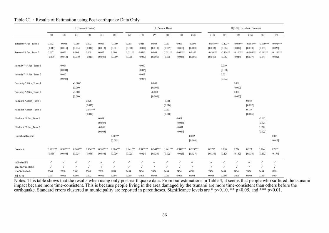
Table C1：Results of Estimation using Post-earthquake Data Only

Notes: This table shows that the results when using only post-earthquake data. From our estimations in Table 4, it seems that people who suffered the tsunami impact became more time-consistent. This is because people living in the area damaged by the tsunami are more time-consistent than others before the earthquake. Standard errors clustered at municipality are reported in parentheses. Significance levels are * p<0.10, ** p<0.05, and *** p<0.01.

(1) (2) (3) (4) (5) (6) (7) (8) (9) (10) (11) (12) (13) (14) (15) (16) (17) (18)

Tsunami*After_Term 1 0.002 -0.004 -0.005 0.002 0.003 -0.000 0.003 0.016 0.005 0.003 0.003 -0.000 -0.089*** -0.123* -0.078** -0.088*** -0.090*** -0.071***

[0.013] [0.015] [0.014] [0.014] [0.013] [0.011] [0.010] [0.014] [0.010] [0.009] [0.010] [0.008] [0.033] [0.064] [0.037] [0.030] [0.033] [0.025]

Tsunami*After_Term 2 0.007 0.006 0.004 0.008 0.007 0.006 0.011** 0.016* 0.009 0.011** 0.010** 0.010* -0.101** -0.154** -0.100** -0.099*** -0.091** -0.114***

[0.009] [0.013] [0.010] [0.010] [0.009] [0.009] [0.005] [0.009] [0.006] [0.005] [0.005] [0.006] [0.041] [0.063] [0.044] [0.037] [0.041] [0.032]

Intensity7 *After_Term 1 0.004 -0.007 0.019

[0.004] [0.005] [0.028]

Intensity7 *After_Term 2 0.000 -0.003 0.031

[0.005] [0.004] [0.022]

Proximity *After_Term 1 -0.000* 0.000 0.000

[0.000] [0.000] [0.000]

Proximity *After_Term 2 -0.000 -0.000 0.000

[0.000] [0.000] [0.000]

Radiation *After_Term 1 0.026 -0.016 0.088

[0.017] [0.016] [0.092]

Radiation *After_Term 2 0.041*** 0.002 0.137

[0.014] [0.010] [0.085]

Blackout *After_Term 1 0.004 0.001 -0.002

[0.007] [0.005] [0.024]

Blackout *After_Term 2 -0.001 -0.001 0.028

[0.005] [0.004] [0.023]

Household Income 0.007** 0.002 0.008

[0.003] [0.003] [0.015]

Constant 0.965*** 0.965*** 0.969*** 0.964*** 0.965*** 0.986*** 0.941*** 0.943*** 0.943*** 0.941*** 0.942*** 0.928*** 0.225* 0.210 0.224 0.223 0.214 0.263*

[0.038] [0.038] [0.038] [0.038] [0.038] [0.036] [0.025] [0.024] [0.026] [0.025] [0.025] [0.027] [0.136] [0.128] [0.142] [0.136] [0.132] [0.154]

Individual FE ✓ ✓ ✓ ✓ ✓ ✓ ✓ ✓ ✓ ✓ ✓ ✓ ✓ ✓ ✓ ✓ ✓ ✓


N of individuals 7560 7560 7560 7560 7560 6894 7454 7454 7454 7454 7454 6798 7454 7454 7454 7454 7454 6798

adj. R-sq 0.001 0.001 0.003 0.002 0.001 0.004 0.005 0.006 0.005 0.005 0.005 0.004 0.005 0.006 0.005 0.005 0.005 0.004


37

Appendix B: Lower and Upper Limits of Time Discounting Rates

In our main estimation, individuals’ time discounting rates are defined by the average value of discounting rate before and after they switch their choice in

the multi-price lists. However, their time discounting rates may take other values within the range of the discount rates before and after the change in selection.

In this section, I test how the results differ depending on our definition of the discounting rate.

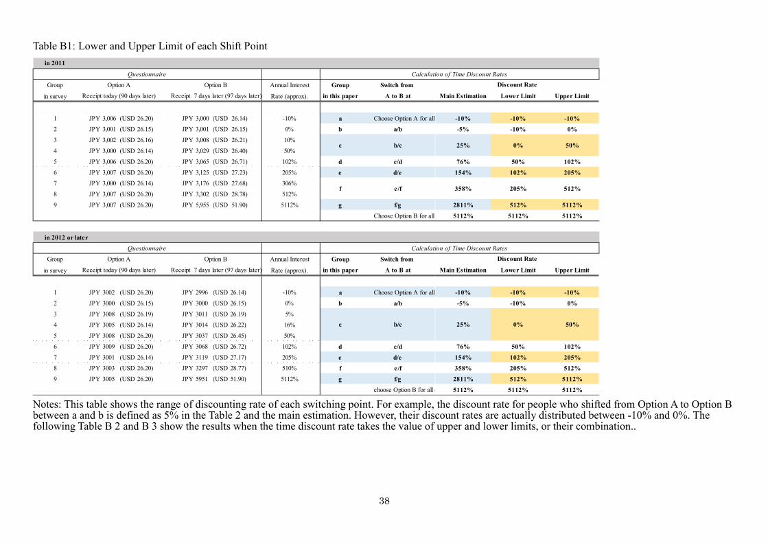
38

Table B1: Lower and Upper Limit of each Shift Point

Notes: This table shows the range of discounting rate of each switching point. For example, the discount rate for people who shifted from Option A to Option B between a and b is defined as 5% in the Table 2 and the main estimation. However, their discount rates are actually distributed between -10% and 0%. The following Table B 2 and B 3 show the results when the time discount rate takes the value of upper and lower limits, or their combination..

Group Annual Interest Group Switch from

in survey Rate (approx). in this paper A to B at Main Estimation Lower Limit Upper Limit

1 JPY 3,006 (USD 26.20) JPY 3,000 (USD 26.14) -10% a Choose Option A for all choices-10% -10% -10%

2 JPY 3,001 (USD 26.15) JPY 3,001 (USD 26.15) 0% b a/b -5% -10% 0%

3 JPY 3,002 (USD 26.16) JPY 3,008 (USD 26.21) 10%

4 JPY 3,000 (USD 26.14) JPY 3,029 (USD 26.40) 50%

5 JPY 3,006 (USD 26.20) JPY 3,065 (USD 26.71) 102% d c/d 76% 50% 102%

6 JPY 3,007 (USD 26.20) JPY 3,125 (USD 27.23) 205% e d/e 154% 102% 205%

7 JPY 3,000 (USD 26.14) JPY 3,176 (USD 27.68) 306%

8 JPY 3,007 (USD 26.20) JPY 3,302 (USD 28.78) 512%

9 JPY 3,007 (USD 26.20) JPY 5,955 (USD 51.90) 5112% g f/g 2811% 512% 5112%

Choose Option B for all choices5112% 5112% 5112%

in 2012 or later

Group Annual Interest Group Switch from

in survey Rate (approx). in this paper A to B at Main Estimation Lower Limit Upper Limit

1 JPY 3002 (USD 26.20) JPY 2996 (USD 26.14) -10% a Choose Option A for all choices-10% -10% -10%

2 JPY 3000 (USD 26.15) JPY 3000 (USD 26.15) 0% b a/b -5% -10% 0%

3 JPY 3008 (USD 26.19) JPY 3011 (USD 26.19) 5%

4 JPY 3005 (USD 26.14) JPY 3014 (USD 26.22) 16%

5 JPY 3008 (USD 26.20) JPY 3037 (USD 26.45) 50%

6 JPY 3009 (USD 26.20) JPY 3068 (USD 26.72) 102% d c/d 76% 50% 102%

7 JPY 3001 (USD 26.14) JPY 3119 (USD 27.17) 205% e d/e 154% 102% 205%

8 JPY 3003 (USD 26.20) JPY 3297 (USD 28.77) 510% f e/f 358% 205% 512%

9 JPY 3005 (USD 26.20) JPY 5951 (USD 51.90) 5112% g f/g 2811% 512% 5112%

choose Option B for all choices5112% 5112% 5112%

25%

f e/f 358%

c b/c

Option B


Questionnaire

c

Option A Option B

Receipt today (90 days later)

Discount Rate

0%

Receipt 7 days later (97 days later)

in 2011

50%

512%

50%


0%

205%

Discount Rate


25%b/c

Questionnaire

Option A

39

Table B2: Changes in Time Preferences with Lower and Upper Limits

Notes: This table reports the results when the time discount rate takes the values of Lower or Upper Limit in Table B1. Panel A and Panel B report the results of Lower Limit and Upper Limit, respectively, which correspond to the results in Table 6. Standard errors clustered at the municipality level are reported in parentheses. Significance levels are * p<0.10, ** p<0.05, and *** p<0.01.

(1) (2) (3) (4) (5) (6) (7) (8) (9) (10) (11) (12) (13) (14) (15) (16) (17) (18)

Panel A: Lower Limit

Tsunami*After_Term 1 -0.015*** -0.024** -0.019** -0.015*** -0.014** -0.020*** -0.008** -0.016 -0.009 -0.009** -0.004 -0.004 0.063*** 0.080 0.069 0.064*** 0.048** 0.066***

[0.005] [0.010] [0.009] [0.005] [0.006] [0.007] [0.004] [0.014] [0.010] [0.004] [0.004] [0.006] [0.017] [0.058] [0.048] [0.018] [0.019] [0.023]

Tsunami*After_Term 2 -0.001 -0.008 -0.005 -0.001 -0.001 -0.008 -0.009*** -0.025* -0.017* -0.009*** -0.005** -0.006* 0.052*** 0.066 0.042 0.053*** 0.044*** 0.053***

[0.009] [0.013] [0.011] [0.009] [0.010] [0.008] [0.003] [0.013] [0.010] [0.003] [0.002] [0.004] [0.017] [0.054] [0.050] [0.017] [0.016] [0.016]

Additional Control Variables Intensity4 Proximity Radiation Blackout Income Intensity4 Proximity Radiation Blackout Income Intensity4 Proximity Radiation Blackout Income

Individual FE ✓ ✓ ✓ ✓ ✓ ✓ ✓ ✓ ✓ ✓ ✓ ✓ ✓ ✓ ✓ ✓ ✓ ✓


N of individuals 9448 9448 9448 9448 9448 8598 9274 9274 9274 9274 9274 8443 9274 9274 9274 9274 9274 8443

adj. R-sq 0.002 0.002 0.002 0.002 0.002 0.002 0.011 0.012 0.011 0.011 0.013 0.012 0.003 0.003 0.003 0.003 0.003 0.003

(1) (2) (3) (4) (5) (6) (7) (8) (9) (10) (11) (12) (13) (14) (15) (16) (17) (18)

Panel B: Upper Limit

Tsunami*After_Term 1 0.008 -0.012 -0.005 0.008 0.008 0.011 -0.022*** -0.025 -0.020 -0.022*** -0.016*** -0.020** 0.058*** 0.076 0.067 0.060*** 0.043** 0.062***

[0.013] [0.020] [0.016] [0.012] [0.013] [0.019] [0.005] [0.020] [0.015] [0.005] [0.005] [0.008] [0.017] [0.057] [0.048] [0.018] [0.018] [0.023]

Tsunami*After_Term 2 0.004 -0.008 -0.008 0.005 0.003 -0.002 -0.009 -0.022 -0.018 -0.009 -0.005 -0.01 0.046*** 0.051 0.017 0.049*** 0.039** 0.048***

[0.016] [0.021] [0.020] [0.015] [0.017] [0.020] [0.011] [0.022] [0.018] [0.011] [0.011] [0.010] [0.017] [0.057] [0.053] [0.018] [0.016] [0.016]


Individual FE ✓ ✓ ✓ ✓ ✓ ✓ ✓ ✓ ✓ ✓ ✓ ✓ ✓ ✓ ✓ ✓ ✓ ✓


N of individuals 9448 9448 9448 9448 9448 8598 9274 9274 9274 9274 9274 8443 9274 9274 9274 9274 9274 8443

adj. R-sq 0.000 0.000 0.000 0.000 0.000 0.001 0.004 0.005 0.004 0.004 0.005 0.005 0.002 0.002 0.002 0.002 0.002 0.002



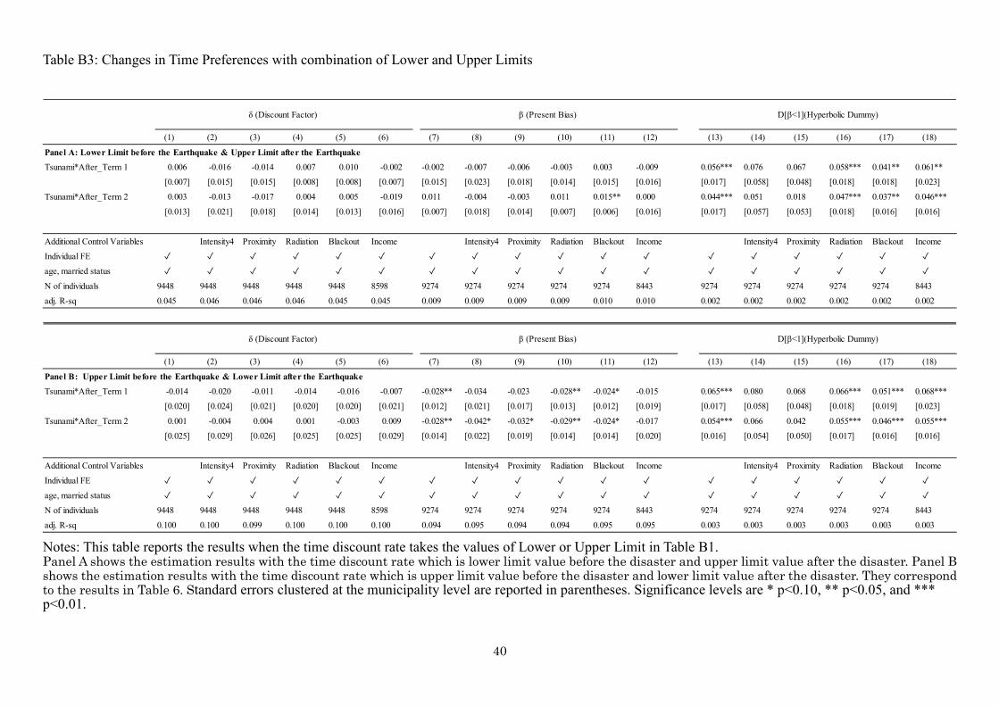
40

Table B3: Changes in Time Preferences with combination of Lower and Upper Limits

Notes: This table reports the results when the time discount rate takes the values of Lower or Upper Limit in Table B1. Panel A shows the estimation results with the time discount rate which is lower limit value before the disaster and upper limit value after the disaster. Panel B shows the estimation results with the time discount rate which is upper limit value before the disaster and lower limit value after the disaster. They correspond to the results in Table 6. Standard errors clustered at the municipality level are reported in parentheses. Significance levels are * p<0.10, ** p<0.05, and *** p<0.01.

(1) (2) (3) (4) (5) (6) (7) (8) (9) (10) (11) (12) (13) (14) (15) (16) (17) (18)

Panel A: Lower Limit before the Earthquake & Upper Limit after the Earthquake

Tsunami*After_Term 1 0.006 -0.016 -0.014 0.007 0.010 -0.002 -0.002 -0.007 -0.006 -0.003 0.003 -0.009 0.056*** 0.076 0.067 0.058*** 0.041** 0.061**

[0.007] [0.015] [0.015] [0.008] [0.008] [0.007] [0.015] [0.023] [0.018] [0.014] [0.015] [0.016] [0.017] [0.058] [0.048] [0.018] [0.018] [0.023]

Tsunami*After_Term 2 0.003 -0.013 -0.017 0.004 0.005 -0.019 0.011 -0.004 -0.003 0.011 0.015** 0.000 0.044*** 0.051 0.018 0.047*** 0.037** 0.046***

[0.013] [0.021] [0.018] [0.014] [0.013] [0.016] [0.007] [0.018] [0.014] [0.007] [0.006] [0.016] [0.017] [0.057] [0.053] [0.018] [0.016] [0.016]


Individual FE ✓ ✓ ✓ ✓ ✓ ✓ ✓ ✓ ✓ ✓ ✓ ✓ ✓ ✓ ✓ ✓ ✓ ✓


N of individuals 9448 9448 9448 9448 9448 8598 9274 9274 9274 9274 9274 8443 9274 9274 9274 9274 9274 8443

adj. R-sq 0.045 0.046 0.046 0.046 0.045 0.045 0.009 0.009 0.009 0.009 0.010 0.010 0.002 0.002 0.002 0.002 0.002 0.002

(1) (2) (3) (4) (5) (6) (7) (8) (9) (10) (11) (12) (13) (14) (15) (16) (17) (18)

Panel B: Upper Limit before the Earthquake & Lower Limit after the Earthquake

Tsunami*After_Term 1 -0.014 -0.020 -0.011 -0.014 -0.016 -0.007 -0.028** -0.034 -0.023 -0.028** -0.024* -0.015 0.065*** 0.080 0.068 0.066*** 0.051*** 0.068***

[0.020] [0.024] [0.021] [0.020] [0.020] [0.021] [0.012] [0.021] [0.017] [0.013] [0.012] [0.019] [0.017] [0.058] [0.048] [0.018] [0.019] [0.023]

Tsunami*After_Term 2 0.001 -0.004 0.004 0.001 -0.003 0.009 -0.028** -0.042* -0.032* -0.029** -0.024* -0.017 0.054*** 0.066 0.042 0.055*** 0.046*** 0.055***

[0.025] [0.029] [0.026] [0.025] [0.025] [0.029] [0.014] [0.022] [0.019] [0.014] [0.014] [0.020] [0.016] [0.054] [0.050] [0.017] [0.016] [0.016]


Individual FE ✓ ✓ ✓ ✓ ✓ ✓ ✓ ✓ ✓ ✓ ✓ ✓ ✓ ✓ ✓ ✓ ✓ ✓


N of individuals 9448 9448 9448 9448 9448 8598 9274 9274 9274 9274 9274 8443 9274 9274 9274 9274 9274 8443

adj. R-sq 0.100 0.100 0.099 0.100 0.100 0.100 0.094 0.095 0.094 0.094 0.095 0.095 0.003 0.003 0.003 0.003 0.003 0.003



Documents

CHANGE IN TIME PREFERENCES: EVIDENCE FROM THE GREAT … · Nobuyoshi Kikuchi, Miki Kohara, and Masaru Sasaki, as well as participants at the Osaka University seminars, 9th conference