Embed Size (px)
Citation preview
D:\web_sites_mine\HIcourseweb new\stats\basics\articles\survival_analysis1\Chan Biostatistics 203_additional_info.docx page 1
Chan Biostatistics 203 - Survival analysis - additional detail
Robin Beaumont Monday, 22 April 2013
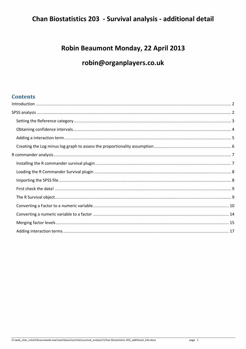
Contents Introduction .................................................................................................................................................................... 2
SPSS analysis ................................................................................................................................................................... 2
Setting the Reference category .................................................................................................................................... 3
Obtaining confidence intervals..................................................................................................................................... 4
Adding a interaction term ............................................................................................................................................ 5
Creating the Log minus log graph to assess the proportionality assumption ................................................................. 6
R commander analysis ..................................................................................................................................................... 7
Installing the R commander survival plugin .................................................................................................................. 7
Loading the R Commander Survival plugin ................................................................................................................... 8
Importing the SPSS file ................................................................................................................................................. 8
First check the data! .................................................................................................................................................... 9
The R Survival object .................................................................................................................................................... 9
Converting a Factor to a numeric variable .................................................................................................................. 10
Converting a numeric variable to a factor .................................................................................................................. 14
Merging factor levels ................................................................................................................................................. 15
Adding interaction terms ........................................................................................................................................... 17
D:\web_sites_mine\HIcourseweb new\stats\basics\articles\survival_analysis1\Chan Biostatistics 203_additional_info.docx page 2
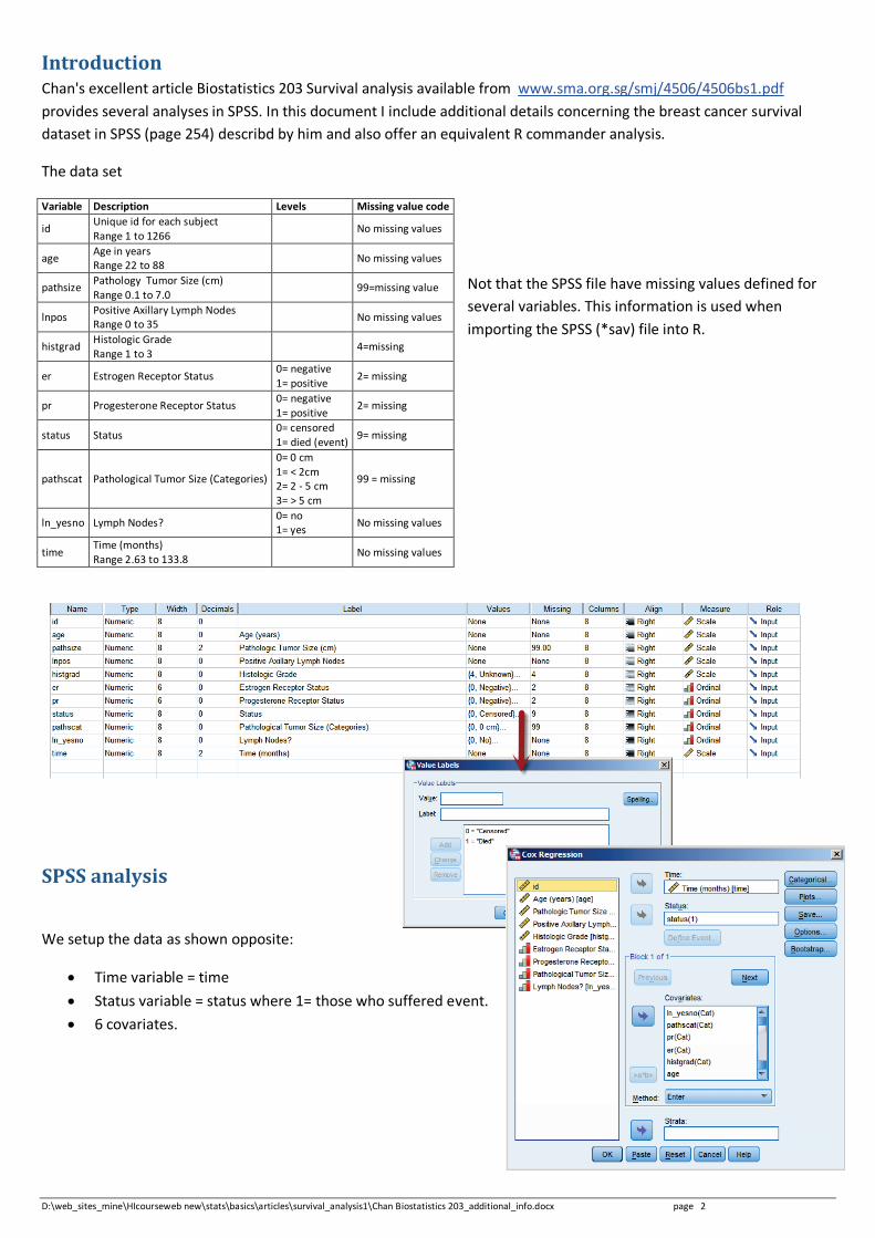
Introduction Chan's excellent article Biostatistics 203 Survival analysis available from www.sma.org.sg/smj/4506/4506bs1.pdf provides several analyses in SPSS. In this document I include additional details concerning the breast cancer survival dataset in SPSS (page 254) describd by him and also offer an equivalent R commander analysis.
The data set
Not that the SPSS file have missing values defined for several variables. This information is used when importing the SPSS (*sav) file into R.
SPSS analysis
We setup the data as shown opposite:
• Time variable = time • Status variable = status where 1= those who suffered event. • 6 covariates.
Variable Description Levels Missing value code
id Unique id for each subject Range 1 to 1266
No missing values
age Age in years Range 22 to 88 No missing values
pathsize Pathology Tumor Size (cm) Range 0.1 to 7.0
99=missing value
lnpos Positive Axillary Lymph Nodes Range 0 to 35 No missing values
histgrad Histologic Grade Range 1 to 3
4=missing
er Estrogen Receptor Status 0= negative 1= positive 2= missing
pr Progesterone Receptor Status 0= negative 1= positive
2= missing
status Status 0= censored 1= died (event) 9= missing
pathscat Pathological Tumor Size (Categories)
0= 0 cm 1= < 2cm 2= 2 - 5 cm 3= > 5 cm
99 = missing
ln_yesno Lymph Nodes? 0= no 1= yes No missing values
time Time (months) Range 2.63 to 133.8 No missing values
D:\web_sites_mine\HIcourseweb new\stats\basics\articles\survival_analysis1\Chan Biostatistics 203_additional_info.docx page 3
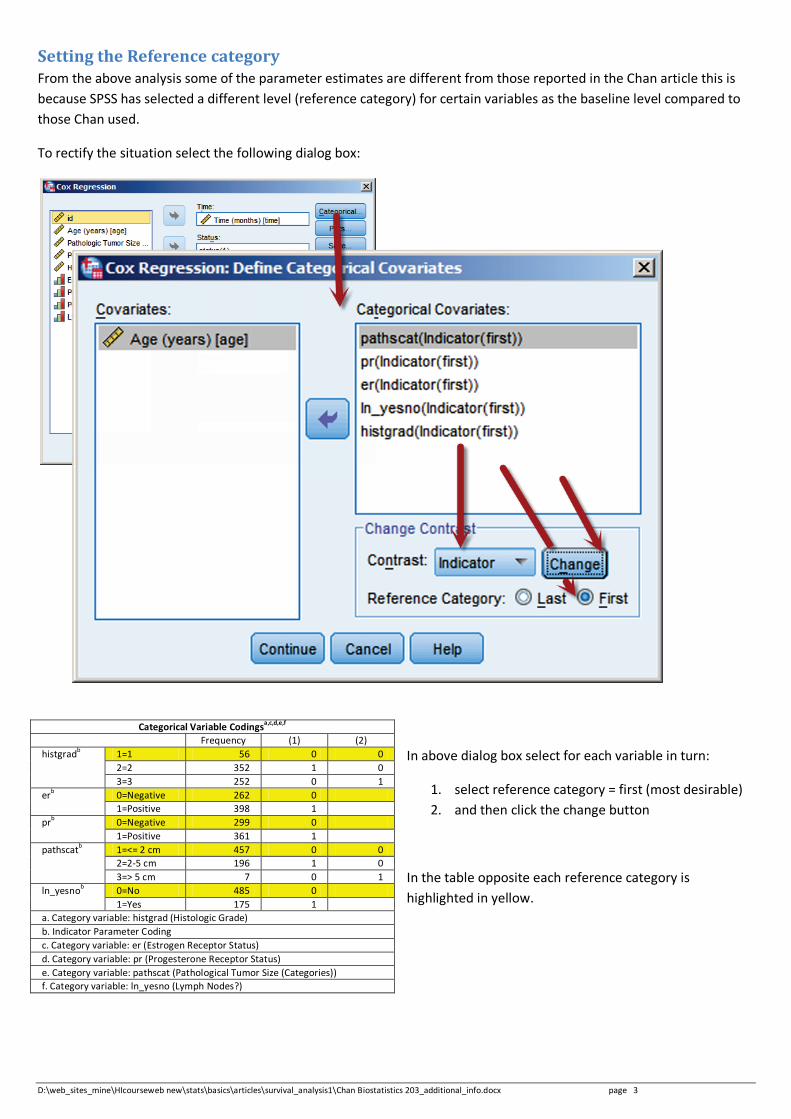
Setting the Reference category From the above analysis some of the parameter estimates are different from those reported in the Chan article this is because SPSS has selected a different level (reference category) for certain variables as the baseline level compared to those Chan used.
To rectify the situation select the following dialog box:
In above dialog box select for each variable in turn:
1. select reference category = first (most desirable) 2. and then click the change button
In the table opposite each reference category is highlighted in yellow.
Categorical Variable Codingsa,c,d,e,f Frequency (1) (2) histgradb 1=1 56 0 0
2=2 352 1 0 3=3 252 0 1
erb 0=Negative 262 0 1=Positive 398 1
prb 0=Negative 299 0 1=Positive 361 1
pathscatb 1=<= 2 cm 457 0 0 2=2-5 cm 196 1 0 3=> 5 cm 7 0 1
ln_yesnob 0=No 485 0 1=Yes 175 1
a. Category variable: histgrad (Histologic Grade) b. Indicator Parameter Coding c. Category variable: er (Estrogen Receptor Status) d. Category variable: pr (Progesterone Receptor Status) e. Category variable: pathscat (Pathological Tumor Size (Categories)) f. Category variable: ln_yesno (Lymph Nodes?)
D:\web_sites_mine\HIcourseweb new\stats\basics\articles\survival_analysis1\Chan Biostatistics 203_additional_info.docx page 4
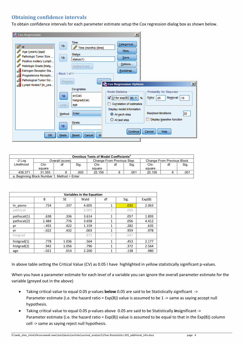
Obtaining confidence intervals To obtain confidence intervals for each parameter estimate setup the Cox regression dialog box as shown below.
Omnibus Tests of Model Coefficientsa -2 Log
Likelihood Overall (score) Change From Previous Step Change From Previous Block
Chi-square
df Sig. Chi-square
df Sig. Chi-square
df Sig.
436.371 31.355 8 .000 25.156 8 .001 25.156 8 .001 a. Beginning Block Number 1. Method = Enter
Variables in the Equation
B SE Wald df Sig. Exp(B)
ln_yesno .724 .337 4.605 1 .032 2.063 pathscat 6.005 2 .050 pathscat(1) .638 .336 3.614 1 .057 1.893 pathscat(2) 1.484 .776 3.658 1 .056 4.412 pr -.455 .422 1.159 1 .282 .635 er -.022 .432 .003 1 .959 .978 histgrad .872 2 .647 histgrad(1) .778 1.036 .564 1 .453 2.177 histgrad(2) .942 1.056 .796 1 .372 2.564 age -.021 .014 2.200 1 .138 .980
In above table setting the Critical Value (CV) as 0.05 I have highlighted in yellow statistically significant p-values.
When you have a parameter estimate for each level of a variable you can ignore the overall parameter estimate for the variable (greyed out in the above)
• Taking critical value to equal 0.05 p-values below 0.05 are said to be Statistically significant -> Parameter estimate (i.e. the hazard ratio = Exp(B)) value is assumed to be 1 -> same as saying accept null hypothesis.
• Taking critical value to equal 0.05 p-values above 0.05 are said to be Statistically insignificant -> Parameter estimate (i.e. the hazard ratio = Exp(B)) value is assumed to be equal to that in the Exp(B)) column cell -> same as saying reject null hypothesis.
D:\web_sites_mine\HIcourseweb new\stats\basics\articles\survival_analysis1\Chan Biostatistics 203_additional_info.docx page 5
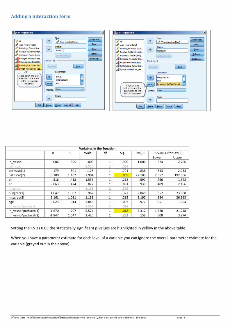
Adding a interaction term
Variables in the Equation
B SE Wald df Sig. Exp(B) 95.0% CI for Exp(B) Lower Upper
ln_yesno .006 .505 .000 1 .990 1.006 .374 2.706 pathscat 8.520 2 .014 pathscat(1) -.179 .501 .128 1 .721 .836 .313 2.233 pathscat(2) 3.100 1.102 7.904 1 .005 22.189 2.557 192.566 pr -.516 .413 1.556 1 .212 .597 .266 1.342 er -.063 .424 .022 1 .881 .939 .409 2.156 histgrad 1.165 2 .559 histgrad(1) 1.047 1.067 .962 1 .327 2.848 .352 23.068 histgrad(2) 1.161 1.081 1.153 1 .283 3.192 .384 26.563 age -.023 .014 2.845 1 .092 .977 .951 1.004 ln_yesno*pathscat 8.564 2 .014 ln_yesno*pathscat(1) 1.670 .707 5.574 1 .018 5.312 1.328 21.248 ln_yesno*pathscat(2) -1.847 1.547 1.425 1 .233 .158 .008 3.274
Setting the CV as 0.05 the statistically significant p-values are highlighted in yellow in the above table
When you have a parameter estimate for each level of a variable you can ignore the overall parameter estimate for the variable (greyed out in the above).
D:\web_sites_mine\HIcourseweb new\stats\basics\articles\survival_analysis1\Chan Biostatistics 203_additional_info.docx page 6
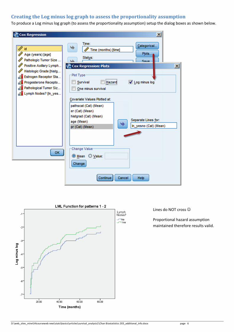
Creating the Log minus log graph to assess the proportionality assumption To produce a Log minus log graph (to assess the proportionality assumption) setup the dialog boxes as shown below.
Lines do NOT cross
Proportional hazard assumption maintained therefore results valid.
D:\web_sites_mine\HIcourseweb new\stats\basics\articles\survival_analysis1\Chan Biostatistics 203_additional_info.docx page 7
R commander analysis This first involves installing and loading the R Commander survival plugin called RcmdPlugin.survival.
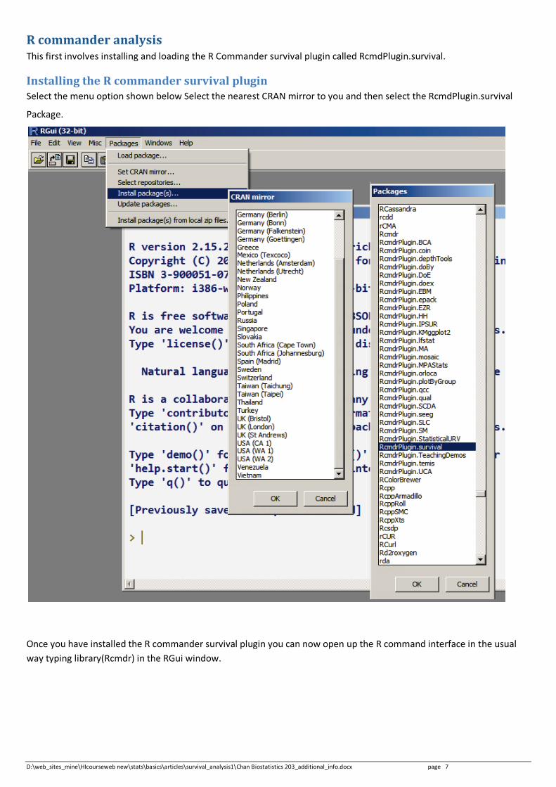
Installing the R commander survival plugin Select the menu option shown below Select the nearest CRAN mirror to you and then select the RcmdPlugin.survival
Package.
Once you have installed the R commander survival plugin you can now open up the R command interface in the usual way typing library(Rcmdr) in the RGui window.
D:\web_sites_mine\HIcourseweb new\stats\basics\articles\survival_analysis1\Chan Biostatistics 203_additional_info.docx page 8
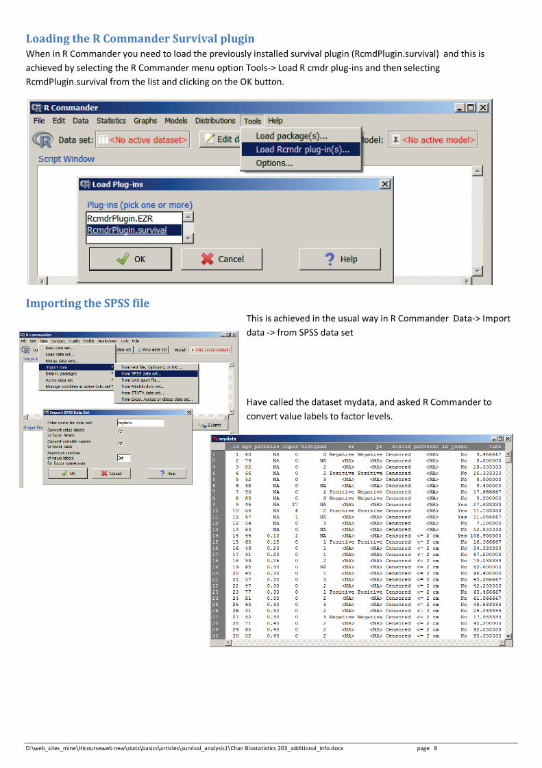
Loading the R Commander Survival plugin When in R Commander you need to load the previously installed survival plugin (RcmdPlugin.survival) and this is achieved by selecting the R Commander menu option Tools-> Load R cmdr plug-ins and then selecting RcmdPlugin.survival from the list and clicking on the OK button.
Importing the SPSS file This is achieved in the usual way in R Commander Data-> Import data -> from SPSS data set
Have called the dataset mydata, and asked R Commander to convert value labels to factor levels.
D:\web_sites_mine\HIcourseweb new\stats\basics\articles\survival_analysis1\Chan Biostatistics 203_additional_info.docx page 9
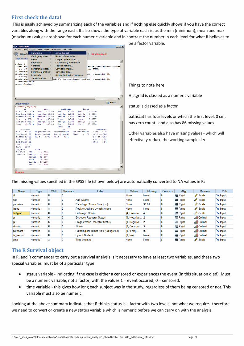
First check the data! This is easily achieved by summarizing each of the variables and if nothing else quickly shows if you have the correct variables along with the range each. It also shows the type of variable each is, as the min (minimum), mean and max (maximum) values are shown for each numeric variable and in contrast the number in each level for what R believes to
be a factor variable.
Things to note here:
Histgrad is classed as a numeric variable
status is classed as a factor
pathscat has four levels or which the first level, 0 cm, has zero count and also has 86 missing values.
Other variables also have missing values - which will effectively reduce the working sample size.
The missing values specified in the SPSS file (shown below) are automatically converted to NA values in R:
The R Survival object In R, and R commander to carry out a survival analysis is it necessary to have at least two variables, and these two special variables must be of a particular type:
• status variable - indicating if the case is either a censored or experiences the event (in this situation died). Must be a numeric variable, not a factor, with the values 1 = event occured; 0 = censored.
• time variable - this gives how long each subject was in the study, regardless of them being censored or not. This variable must also be numeric.
Looking at the above summary indicates that R thinks status is a factor with two levels, not what we require. therefore we need to convert or create a new status variable which is numeric before we can carry on with the analysis.
D:\web_sites_mine\HIcourseweb new\stats\basics\articles\survival_analysis1\Chan Biostatistics 203_additional_info.docx page 10
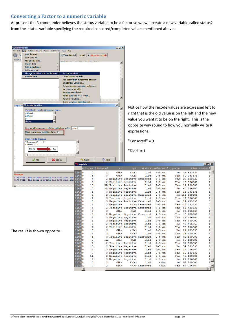
Converting a Factor to a numeric variable At present the R commander believes the status variable to be a factor so we will create a new variable called status2 from the status variable specifying the required censored/completed values mentioned above.
Notice how the recode values are expressed left to right that is the old value is on the left and the new value you want it to be on the right. This is the opposite way round to how you normally write R expressions.
"Censored" = 0
"Died" = 1
The result is shown opposite.
D:\web_sites_mine\HIcourseweb new\stats\basics\articles\survival_analysis1\Chan Biostatistics 203_additional_info.docx page 11
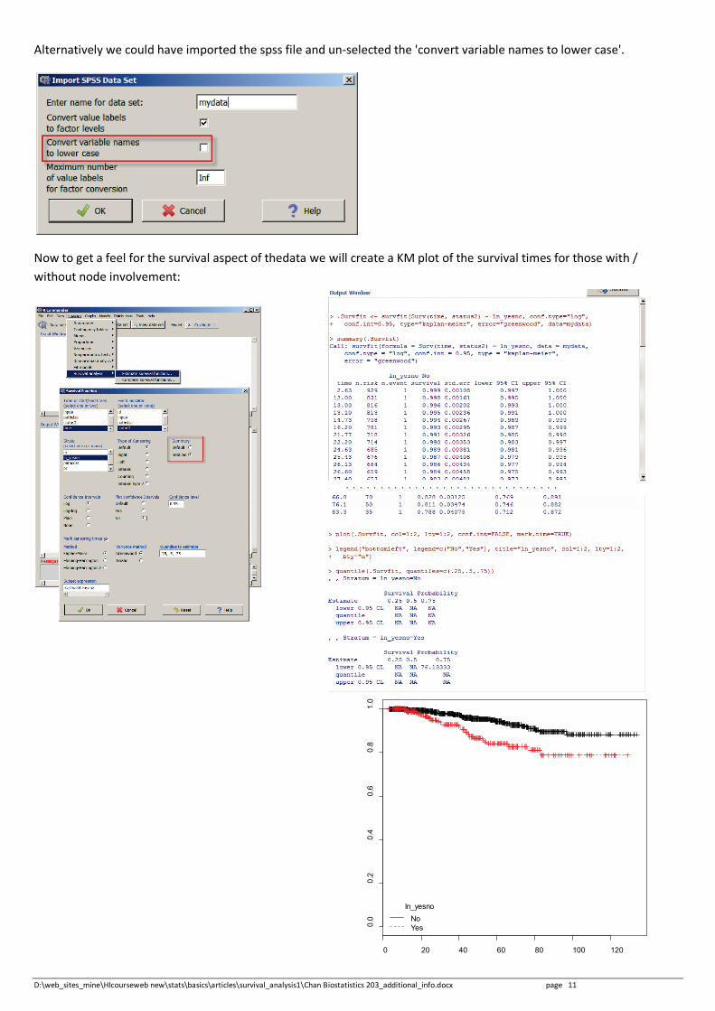
Alternatively we could have imported the spss file and un-selected the 'convert variable names to lower case'.
Now to get a feel for the survival aspect of thedata we will create a KM plot of the survival times for those with / without node involvement:
0 20 40 60 80 100 120
0.0
0.2
0.4
0.6
0.8
1.0
ln_yesnoNoYes
D:\web_sites_mine\HIcourseweb new\stats\basics\articles\survival_analysis1\Chan Biostatistics 203_additional_info.docx page 12
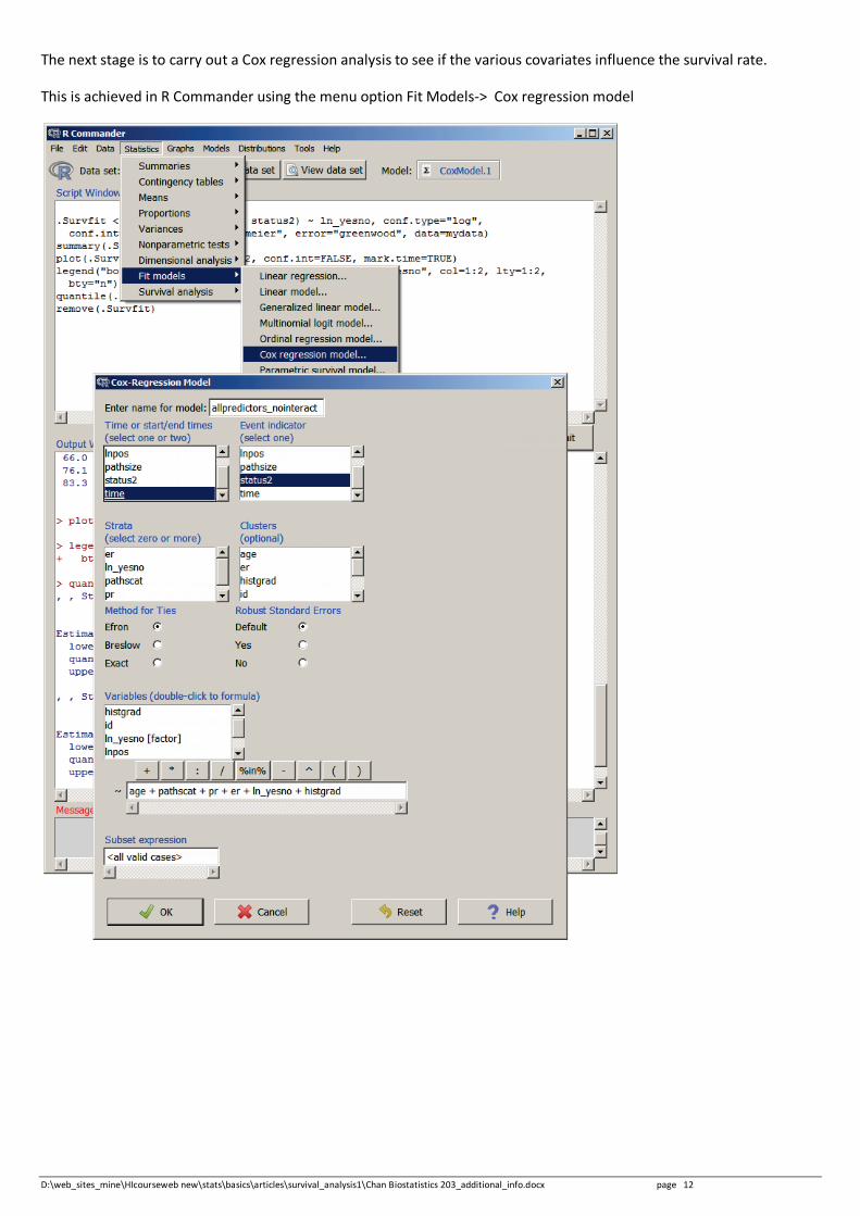
The next stage is to carry out a Cox regression analysis to see if the various covariates influence the survival rate.
This is achieved in R Commander using the menu option Fit Models-> Cox regression model
D:\web_sites_mine\HIcourseweb new\stats\basics\articles\survival_analysis1\Chan Biostatistics 203_additional_info.docx page 13
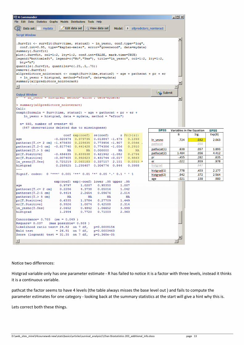
Notice two differences:
Histgrad variable only has one parameter estimate - R has failed to notice it is a factor with three levels, instead it thinks it is a continuous variable.
pathcat the factor seems to have 4 levels (the table always misses the base level out ) and fails to compute the parameter estimates for one category - looking back at the summary statistics at the start will give a hint why this is.
Lets correct both these things.
D:\web_sites_mine\HIcourseweb new\stats\basics\articles\survival_analysis1\Chan Biostatistics 203_additional_info.docx page 14
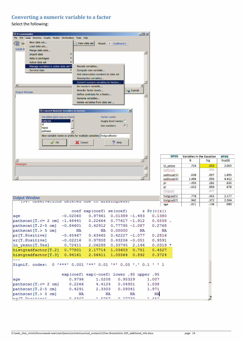
Converting a numeric variable to a factor Select the following:
D:\web_sites_mine\HIcourseweb new\stats\basics\articles\survival_analysis1\Chan Biostatistics 203_additional_info.docx page 15
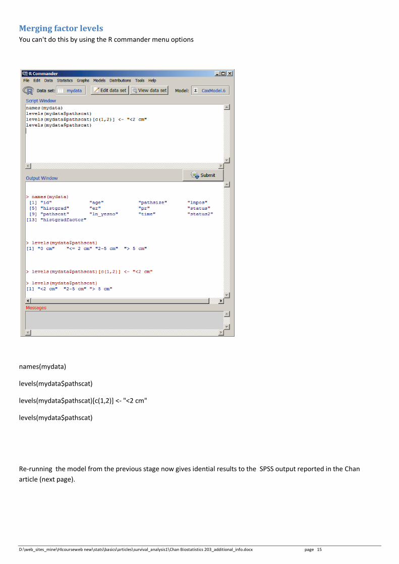
Merging factor levels You can't do this by using the R commander menu options
names(mydata)
levels(mydata$pathscat)
levels(mydata$pathscat)[c(1,2)] <- "<2 cm"
levels(mydata$pathscat)
Re-running the model from the previous stage now gives idential results to the SPSS output reported in the Chan article (next page).
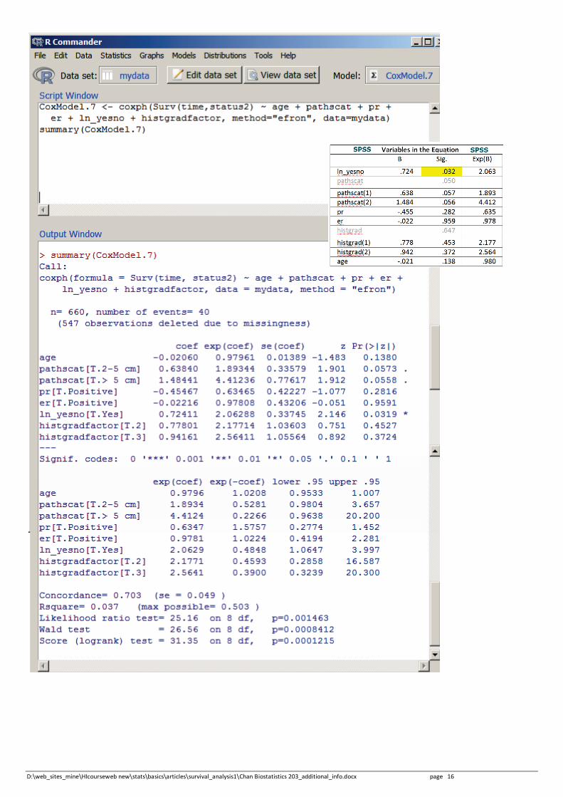
D:\web_sites_mine\HIcourseweb new\stats\basics\articles\survival_analysis1\Chan Biostatistics 203_additional_info.docx page 16
D:\web_sites_mine\HIcourseweb new\stats\basics\articles\survival_analysis1\Chan Biostatistics 203_additional_info.docx page 17
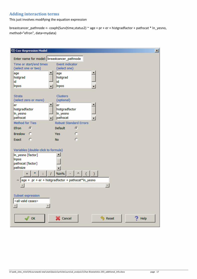
Adding interaction terms This just involves modifying the equation expression
breastcancer_pathnode <- coxph(Surv(time,status2) ~ age + pr + er + histgradfactor + pathscat * ln_yesno, method="efron", data=mydata)
D:\web_sites_mine\HIcourseweb new\stats\basics\articles\survival_analysis1\Chan Biostatistics 203_additional_info.docx page 18
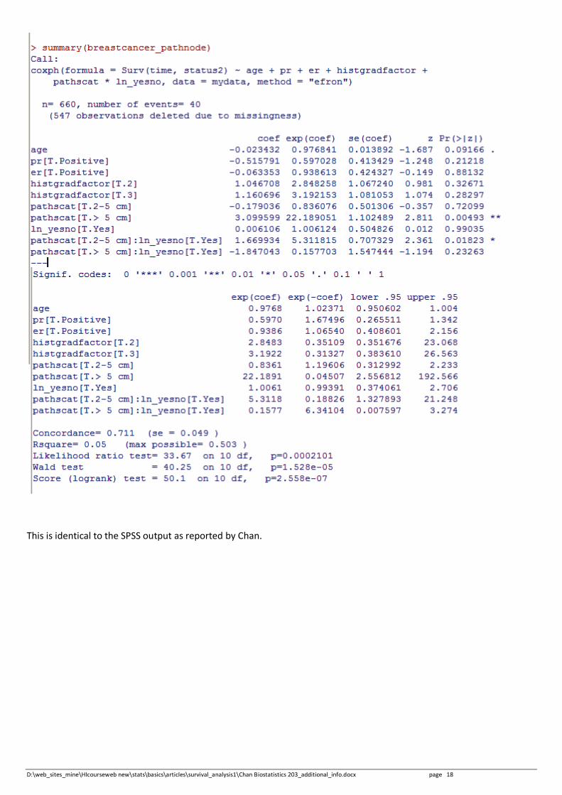
This is identical to the SPSS output as reported by Chan.