Embed Size (px)
Citation preview
Chameleon subwoofer arrays
Adaptable loudspeaker polar responses for improved control in the low-frequency band
Adam Hill
Audio Research Laboratory
School of Computer Science & Electronic Engineering
University of Essex, Colchester, UK
11 October 2011
Problem statement
Develop a low-frequency sound reproduction
system capable of delivering a consistent spectral
and temporal response across a wide-area.

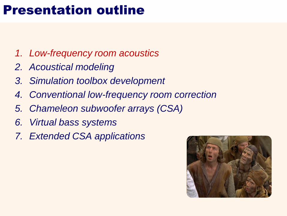
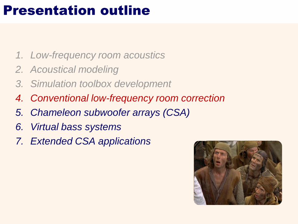
Presentation outline
1. Low-frequency room acoustics
2. Acoustical modeling
3. Simulation toolbox development
4. Conventional low-frequency room correction
5. Chameleon subwoofer arrays (CSA)
6. Virtual bass systems
7. Extended CSA applications
Presentation outline
1. Low-frequency room acoustics
2. Acoustical modeling
3. Simulation toolbox development
4. Conventional low-frequency room correction
5. Chameleon subwoofer arrays (CSA)
6. Virtual bass systems
7. Extended CSA applications
Low-frequency room acoustics [1/5]
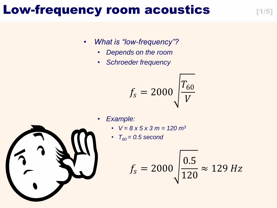
• What is “low-frequency”?
• Depends on the room
• Schroeder frequency
• Example:
• V = 8 x 5 x 3 m = 120 m3
• T60 = 0.5 second
𝑓𝑠 = 2000 𝑇60
𝑉
𝑓𝑠 = 2000 0.5
120≈ 129 𝐻𝑧
Low-frequency room acoustics [2/5]
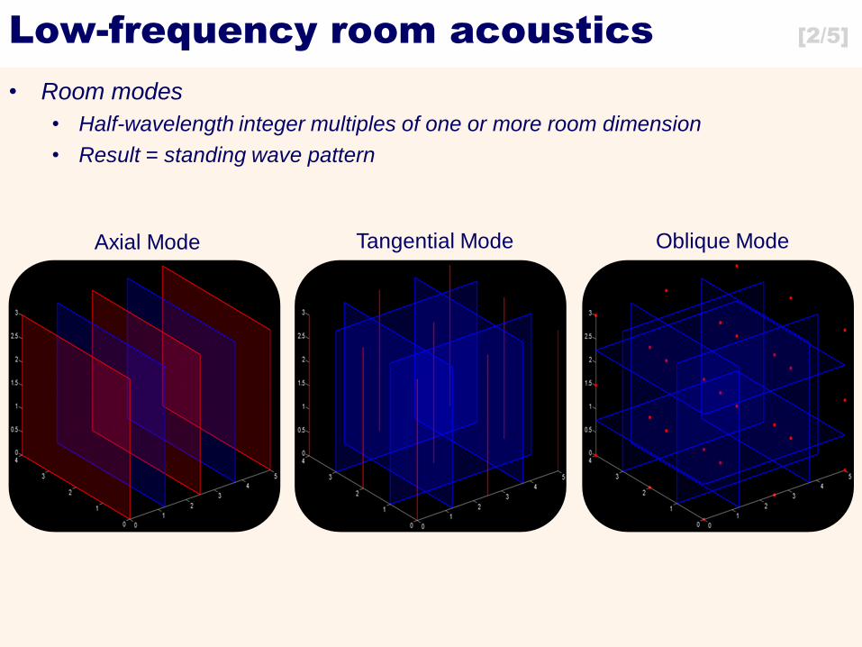
• Room modes
• Half-wavelength integer multiples of one or more room dimension
• Result = standing wave pattern
Axial Mode Tangential Mode Oblique Mode
Low-frequency room acoustics [3/5]
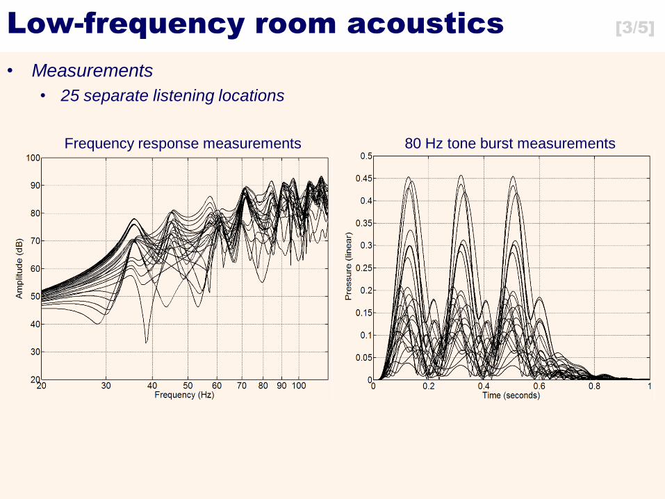
• Measurements
• 25 separate listening locations
Frequency response measurements 80 Hz tone burst measurements
Low-frequency room acoustics [4/5]
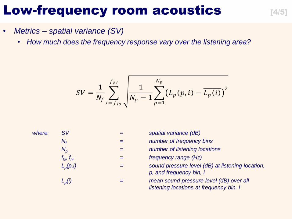
• Metrics – spatial variance (SV)
• How much does the frequency response vary over the listening area?
where: SV = spatial variance (dB)
Nf = number of frequency bins
Np = number of listening locations
flo, fhi = frequency range (Hz)
Lp(p,i) = sound pressure level (dB) at listening location,
p, and frequency bin, i
Lp(i) = mean sound pressure level (dB) over all
listening locations at frequency bin, i
𝑆𝑉 =1
𝑁𝑓
1
𝑁𝑝 − 1 𝐿𝑝 𝑝, 𝑖 − 𝐿𝑝 𝑖
2
𝑁𝑝
𝑝=1
𝑓ℎ𝑖
𝑖= 𝑓𝑙𝑜
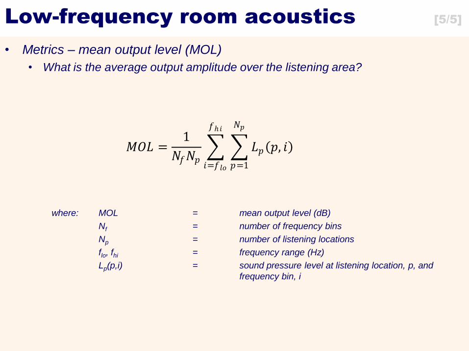
Low-frequency room acoustics [5/5]
• Metrics – mean output level (MOL)
• What is the average output amplitude over the listening area?
where: MOL = mean output level (dB)
Nf = number of frequency bins
Np = number of listening locations
flo, fhi = frequency range (Hz)
Lp(p,i) = sound pressure level at listening location, p, and
frequency bin, i
𝑀𝑂𝐿 =1
𝑁𝑓𝑁𝑝 𝐿𝑝 𝑝, 𝑖
𝑁𝑝
𝑝=1
𝑓ℎ𝑖
𝑖=𝑓𝑙𝑜
Presentation outline
1. Low-frequency room acoustics
2. Acoustical modeling
3. Simulation toolbox development
4. Conventional low-frequency room correction
5. Chameleon subwoofer arrays (CSA)
6. Virtual bass systems
7. Extended CSA applications
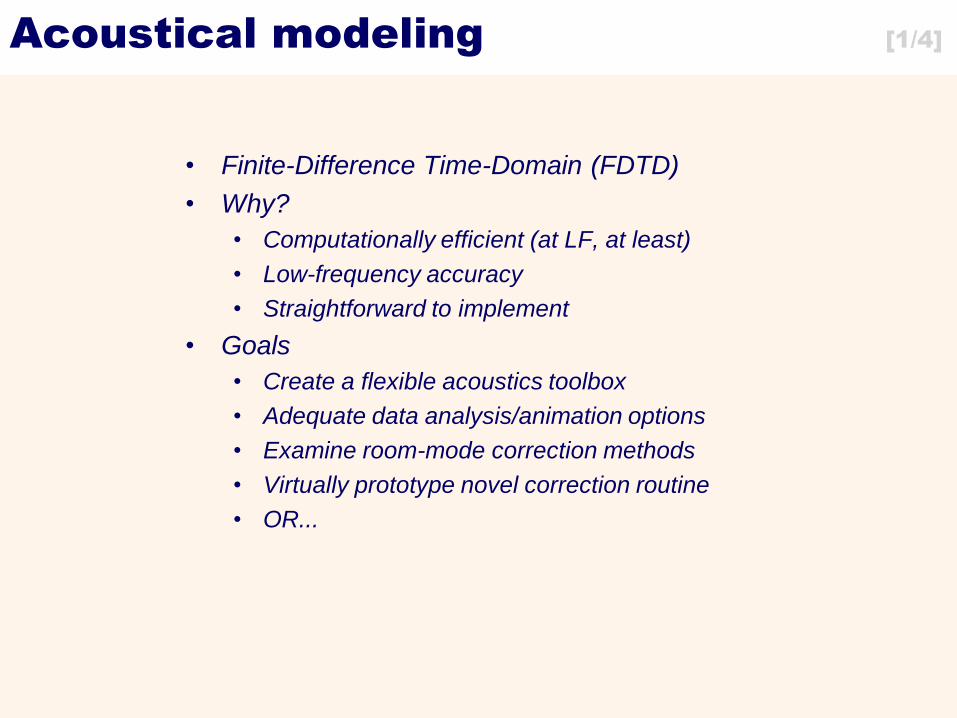
Acoustical modeling [1/4]
• Finite-Difference Time-Domain (FDTD)
• Why?
• Computationally efficient (at LF, at least)
• Low-frequency accuracy
• Straightforward to implement
• Goals
• Create a flexible acoustics toolbox
• Adequate data analysis/animation options
• Examine room-mode correction methods
• Virtually prototype novel correction routine
• OR...
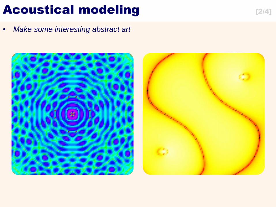
Acoustical modeling [2/4]
• Make some interesting abstract art
Acoustical modeling [3/4]
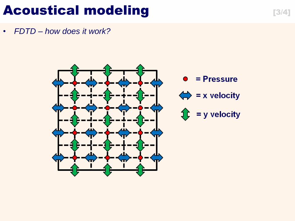
• FDTD – how does it work?
Acoustical modeling [4/4]
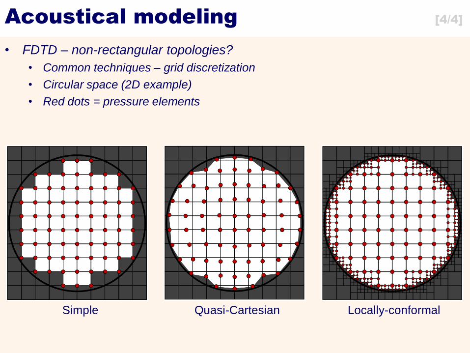
• FDTD – non-rectangular topologies?
• Common techniques – grid discretization
• Circular space (2D example)
• Red dots = pressure elements
Simple Quasi-Cartesian Locally-conformal

Presentation outline
1. Low-frequency room acoustics
2. Acoustical modeling
3. Simulation toolbox development
4. Conventional low-frequency room correction
5. Chameleon subwoofer arrays (CSA)
6. Virtual bass systems
7. Extended CSA applications
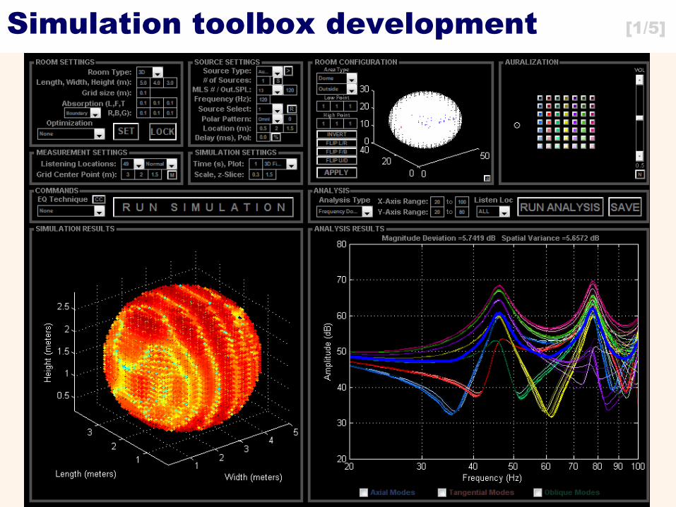
Simulation toolbox development [1/5]
Simulation toolbox development [2/5]
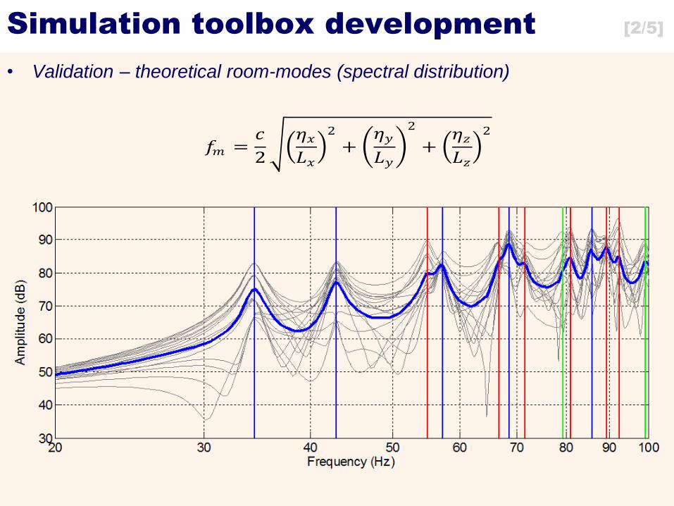
• Validation – theoretical room-modes (spectral distribution)
𝑓𝑚 =𝑐
2
𝜂𝑥𝐿𝑥
2
+ 𝜂𝑦𝐿𝑦
2
+ 𝜂𝑧𝐿𝑧
2
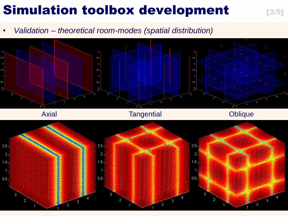
Simulation toolbox development [3/5]
• Validation – theoretical room-modes (spatial distribution)
Axial Tangential Oblique
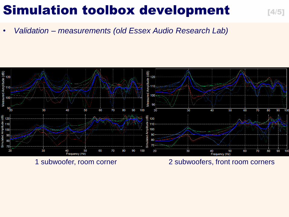
Simulation toolbox development [4/5]
• Validation – measurements (old Essex Audio Research Lab)
1 subwoofer, room corner 2 subwoofers, front room corners
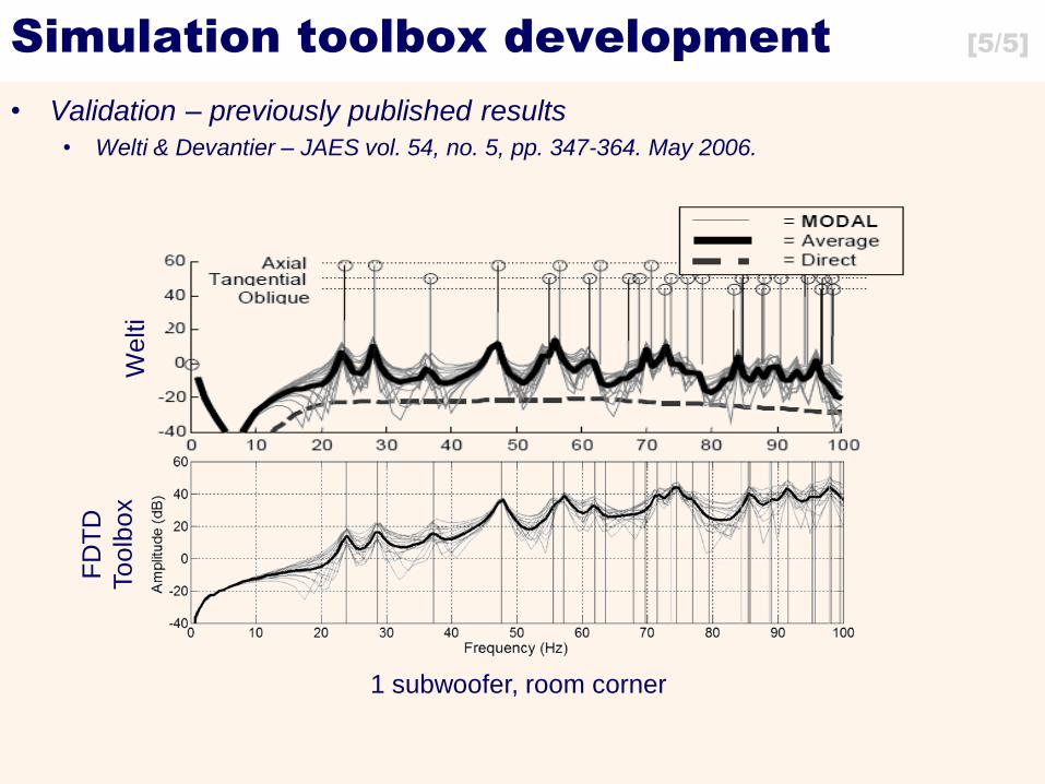
Simulation toolbox development [5/5]
• Validation – previously published results
• Welti & Devantier – JAES vol. 54, no. 5, pp. 347-364. May 2006.
We
lti
FD
TD
To
olb
ox
1 subwoofer, room corner
Presentation outline
1. Low-frequency room acoustics
2. Acoustical modeling
3. Simulation toolbox development
4. Conventional low-frequency room correction
5. Chameleon subwoofer arrays (CSA)
6. Virtual bass systems
7. Extended CSA applications
Conventional correction [2/8]
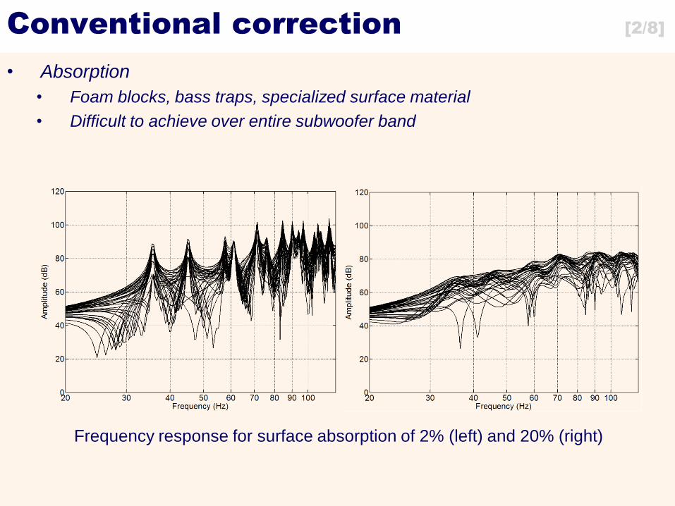
• Absorption
• Foam blocks, bass traps, specialized surface material
• Difficult to achieve over entire subwoofer band
Frequency response for surface absorption of 2% (left) and 20% (right)
Conventional correction [3/8]
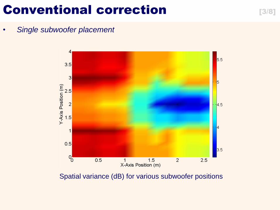
• Single subwoofer placement
Spatial variance (dB) for various subwoofer positions
Conventional correction [4/8]
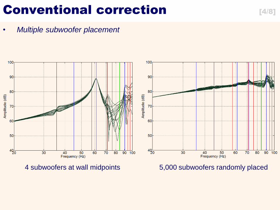
• Multiple subwoofer placement
4 subwoofers at wall midpoints 5,000 subwoofers randomly placed
Conventional correction [5/8]
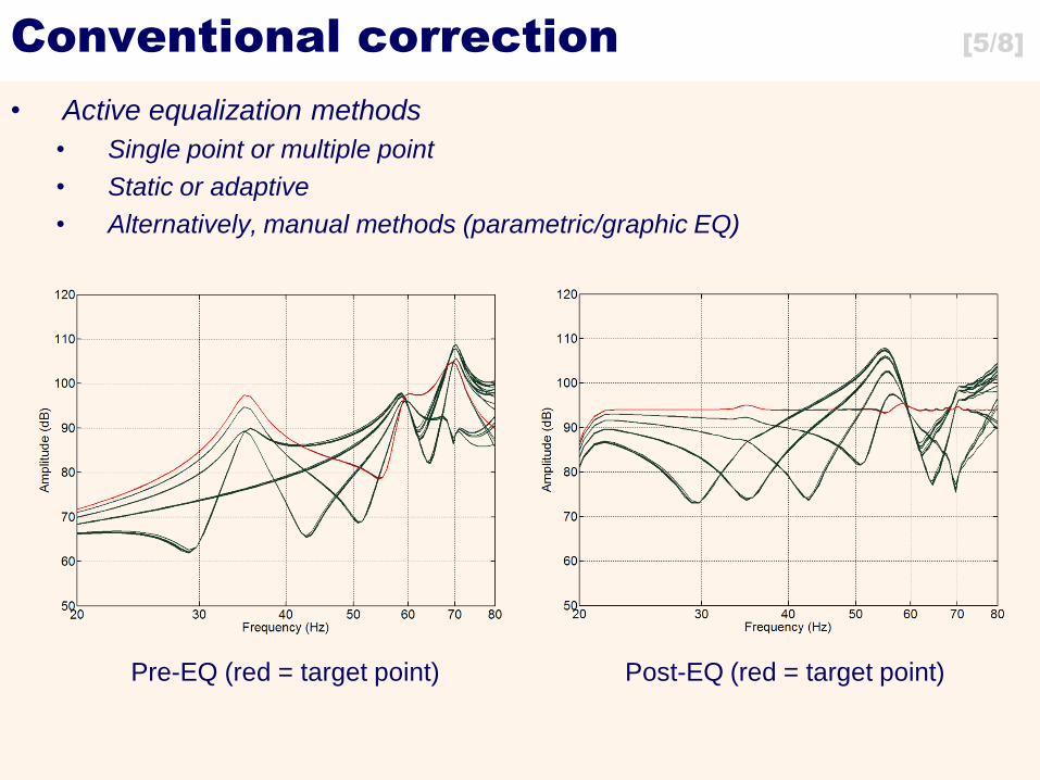
• Active equalization methods
• Single point or multiple point
• Static or adaptive
• Alternatively, manual methods (parametric/graphic EQ)
Pre-EQ (red = target point) Post-EQ (red = target point)
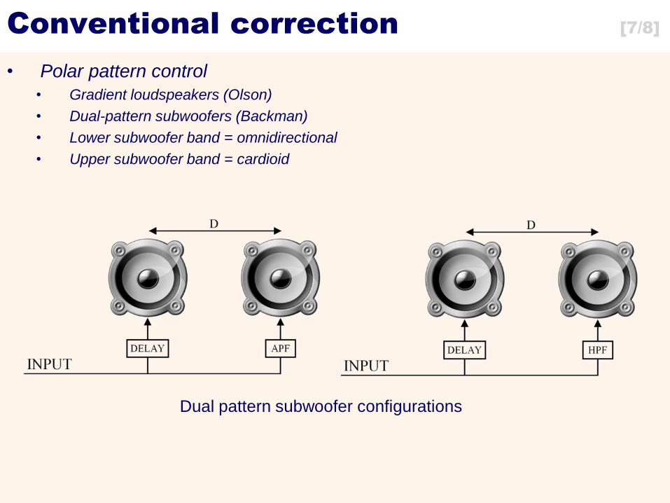
Conventional correction [7/8]
• Polar pattern control
• Gradient loudspeakers (Olson)
• Dual-pattern subwoofers (Backman)
• Lower subwoofer band = omnidirectional
• Upper subwoofer band = cardioid
Dual pattern subwoofer configurations
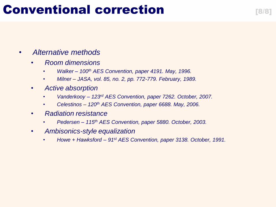
Conventional correction [8/8]
• Alternative methods
• Room dimensions
• Walker – 100th AES Convention, paper 4191. May, 1996.
• Milner – JASA, vol. 85, no. 2, pp. 772-779. February, 1989.
• Active absorption
• Vanderkooy – 123rd AES Convention, paper 7262. October, 2007.
• Celestinos – 120th AES Convention, paper 6688. May, 2006.
• Radiation resistance
• Pedersen – 115th AES Convention, paper 5880. October, 2003.
• Ambisonics-style equalization
• Howe + Hawksford – 91st AES Convention, paper 3138. October, 1991.
Presentation outline
1. Low-frequency room acoustics
2. Acoustical modeling
3. Simulation toolbox development
4. Conventional low-frequency room correction
5. Chameleon subwoofer arrays (CSA)
6. Virtual bass systems
7. Extended CSA applications
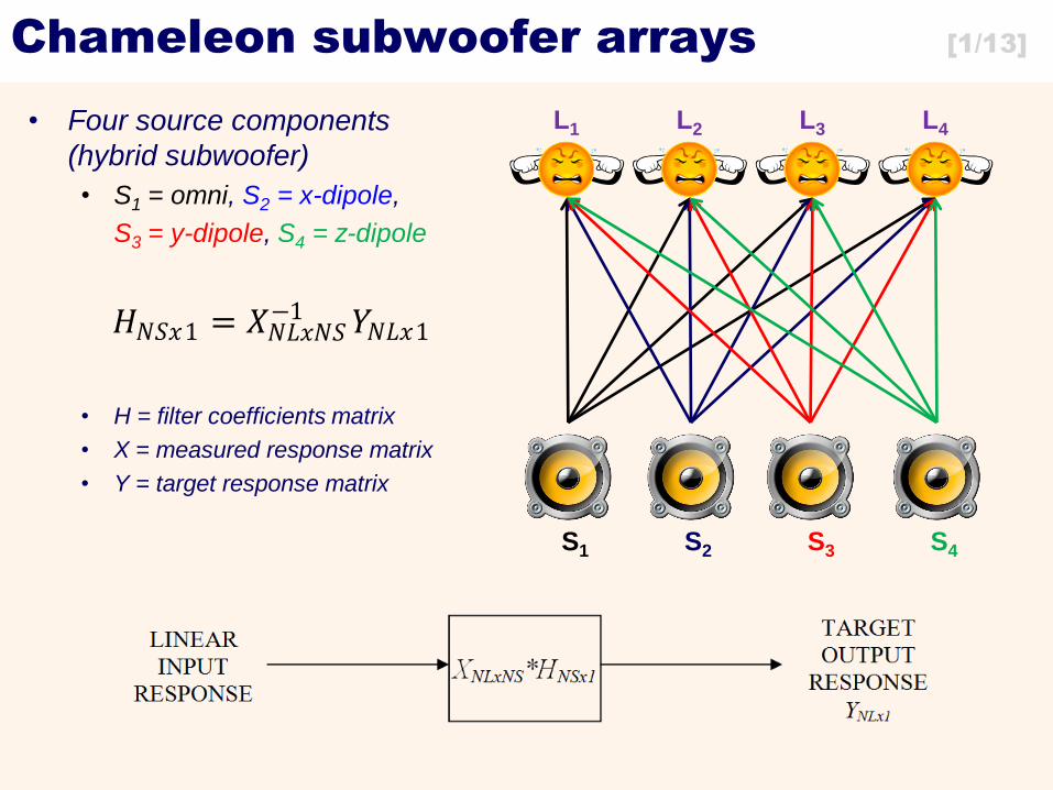
Chameleon subwoofer arrays [1/13]
• Four source components
(hybrid subwoofer)
• S1 = omni, S2 = x-dipole,
S3 = y-dipole, S4 = z-dipole
• H = filter coefficients matrix
• X = measured response matrix
• Y = target response matrix
S1 S2 S3 S4
L1 L2 L3 L4
𝐻𝑁𝑆𝑥1 = 𝑋𝑁𝐿𝑥𝑁𝑆−1 𝑌𝑁𝐿𝑥1
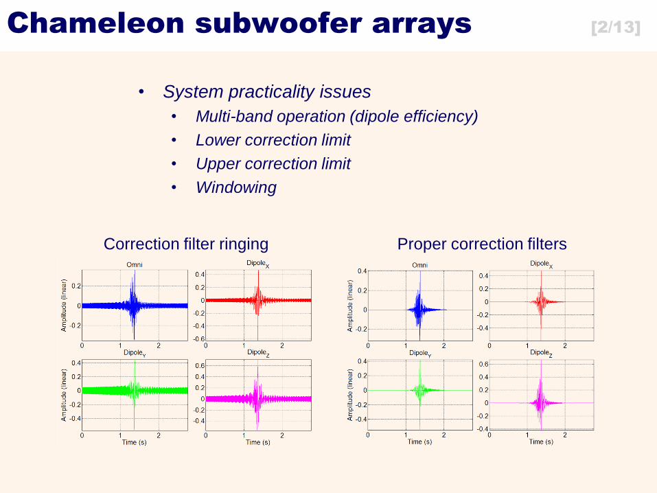
Chameleon subwoofer arrays [2/13]
• System practicality issues
• Multi-band operation (dipole efficiency)
• Lower correction limit
• Upper correction limit
• Windowing
Correction filter ringing Proper correction filters
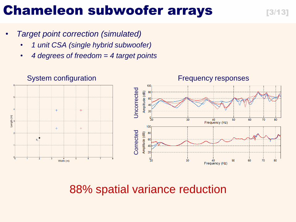
Chameleon subwoofer arrays [3/13]
• Target point correction (simulated)
• 1 unit CSA (single hybrid subwoofer)
• 4 degrees of freedom = 4 target points
System configuration Frequency responses
Uncorr
ecte
d
Corr
ecte
d
88% spatial variance reduction
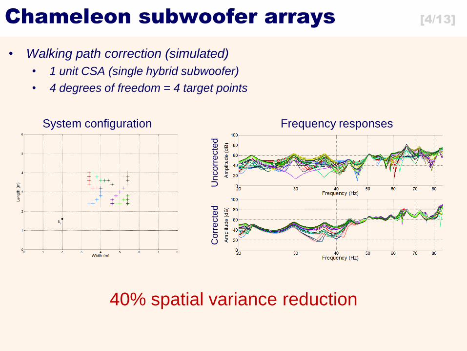
Chameleon subwoofer arrays [4/13]
• Walking path correction (simulated)
• 1 unit CSA (single hybrid subwoofer)
• 4 degrees of freedom = 4 target points
System configuration Frequency responses
Uncorr
ecte
d
Corr
ecte
d
40% spatial variance reduction
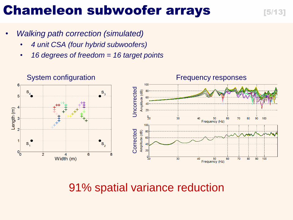
Chameleon subwoofer arrays [5/13]
• Walking path correction (simulated)
• 4 unit CSA (four hybrid subwoofers)
• 16 degrees of freedom = 16 target points
System configuration Frequency responses
Uncorr
ecte
d
Corr
ecte
d
91% spatial variance reduction
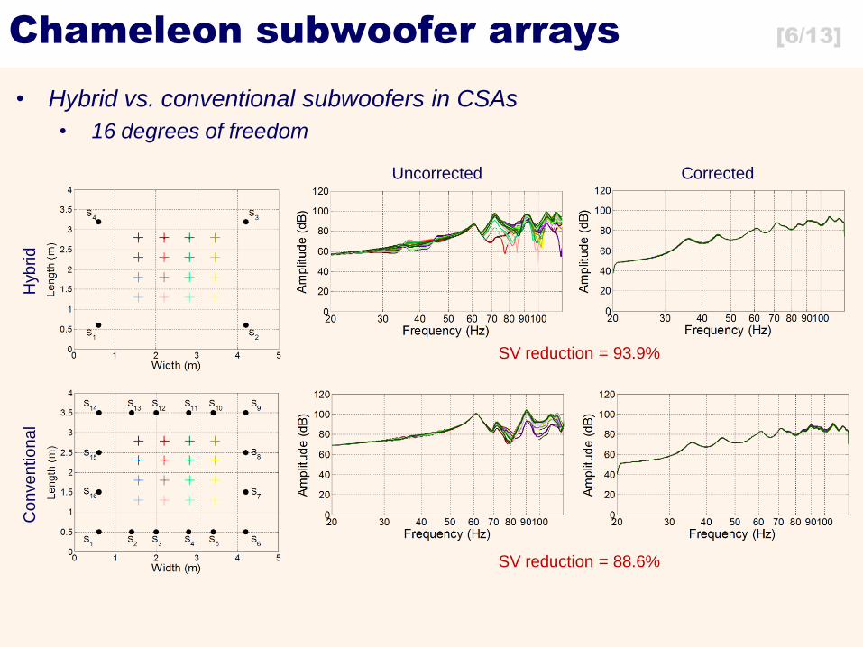
Chameleon subwoofer arrays [6/13]
• Hybrid vs. conventional subwoofers in CSAs
• 16 degrees of freedom
Hyb
rid
Conventional
Uncorrected Corrected
SV reduction = 93.9%
SV reduction = 88.6%
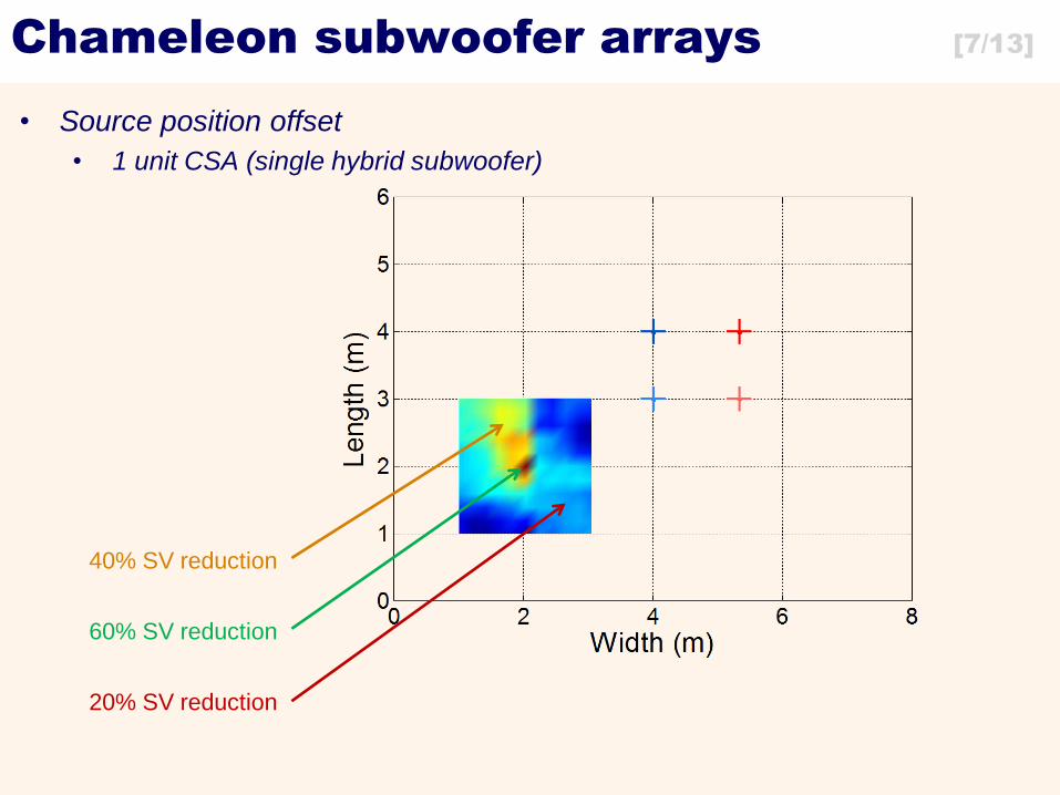
Chameleon subwoofer arrays [7/13]
• Source position offset
• 1 unit CSA (single hybrid subwoofer)
60% SV reduction
40% SV reduction
20% SV reduction
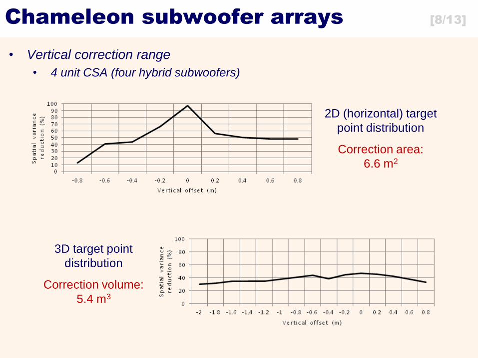
Chameleon subwoofer arrays [8/13]
• Vertical correction range
• 4 unit CSA (four hybrid subwoofers)
2D (horizontal) target
point distribution
3D target point
distribution
Correction area:
6.6 m2
Correction volume:
5.4 m3
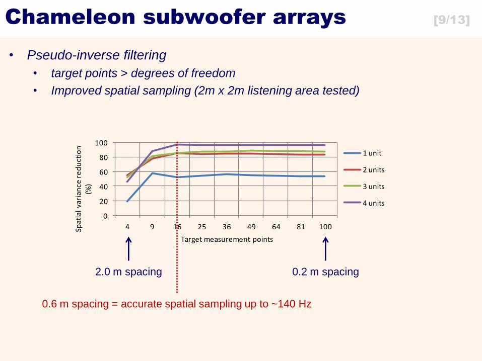
Chameleon subwoofer arrays [9/13]
• Pseudo-inverse filtering
• target points > degrees of freedom
• Improved spatial sampling (2m x 2m listening area tested)
0
20
40
60
80
100
4 9 16 25 36 49 64 81 100Spat
ial
vari
ance
re
du
ctio
n
(%)
Target measurement points
1 unit
2 units
3 units
4 units
2.0 m spacing 0.2 m spacing
0.6 m spacing = accurate spatial sampling up to ~140 Hz
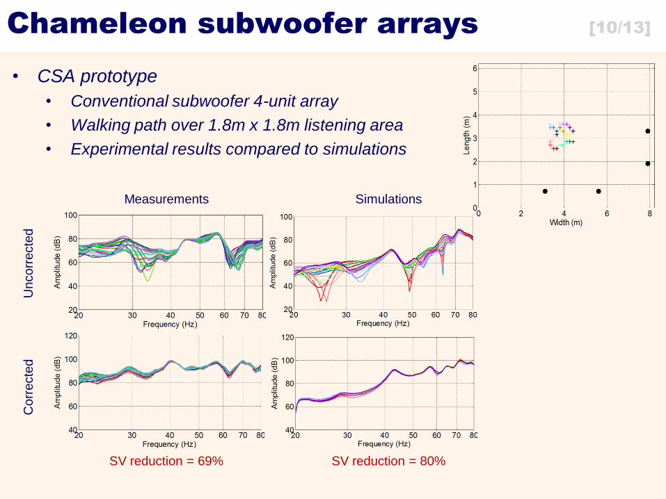
Chameleon subwoofer arrays [10/13]
• CSA prototype
• Conventional subwoofer 4-unit array
• Walking path over 1.8m x 1.8m listening area
• Experimental results compared to simulations
Uncorr
ecte
d
Corr
ecte
d
Measurements Simulations
SV reduction = 69% SV reduction = 80%
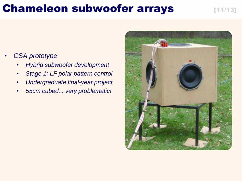
Chameleon subwoofer arrays [11/13]
• CSA prototype
• Hybrid subwoofer development
• Stage 1: LF polar pattern control
• Undergraduate final-year project
• 55cm cubed... very problematic!
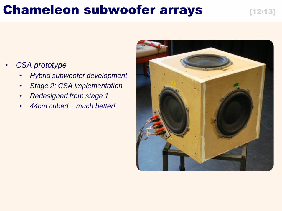
Chameleon subwoofer arrays [12/13]
• CSA prototype
• Hybrid subwoofer development
• Stage 2: CSA implementation
• Redesigned from stage 1
• 44cm cubed... much better!
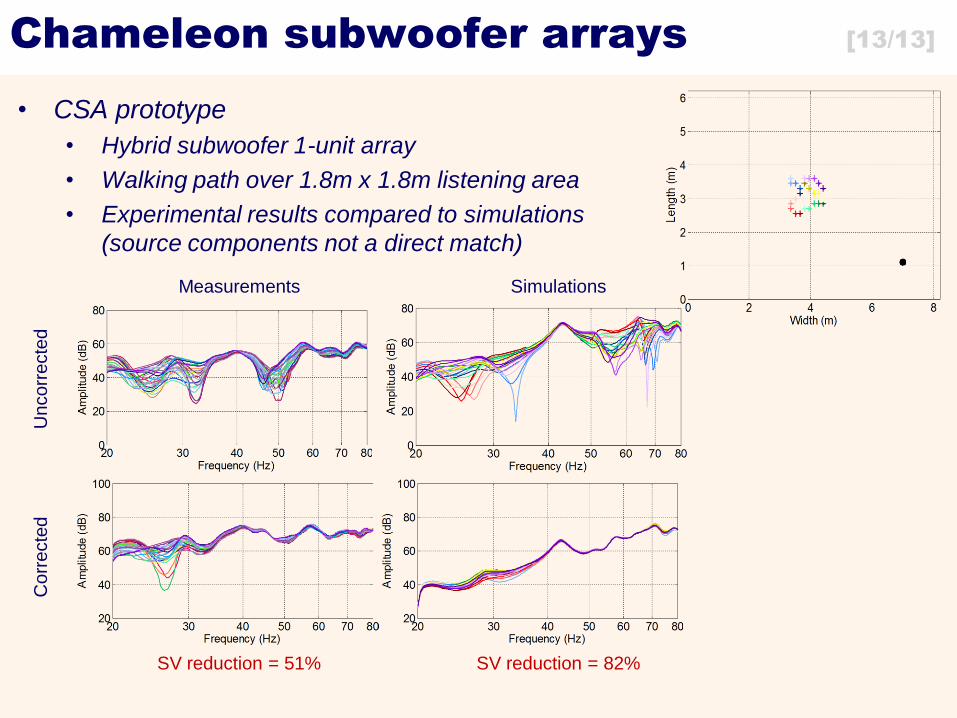
Chameleon subwoofer arrays [13/13]
• CSA prototype
• Hybrid subwoofer 1-unit array
• Walking path over 1.8m x 1.8m listening area
• Experimental results compared to simulations
(source components not a direct match)
Uncorr
ecte
d
Corr
ecte
d
Measurements Simulations
SV reduction = 51% SV reduction = 82%

Presentation outline
1. Low-frequency room acoustics
2. Acoustical modeling
3. Simulation toolbox development
4. Conventional low-frequency room correction
5. Chameleon subwoofer arrays (CSA)
6. Virtual bass systems
7. Extended CSA applications
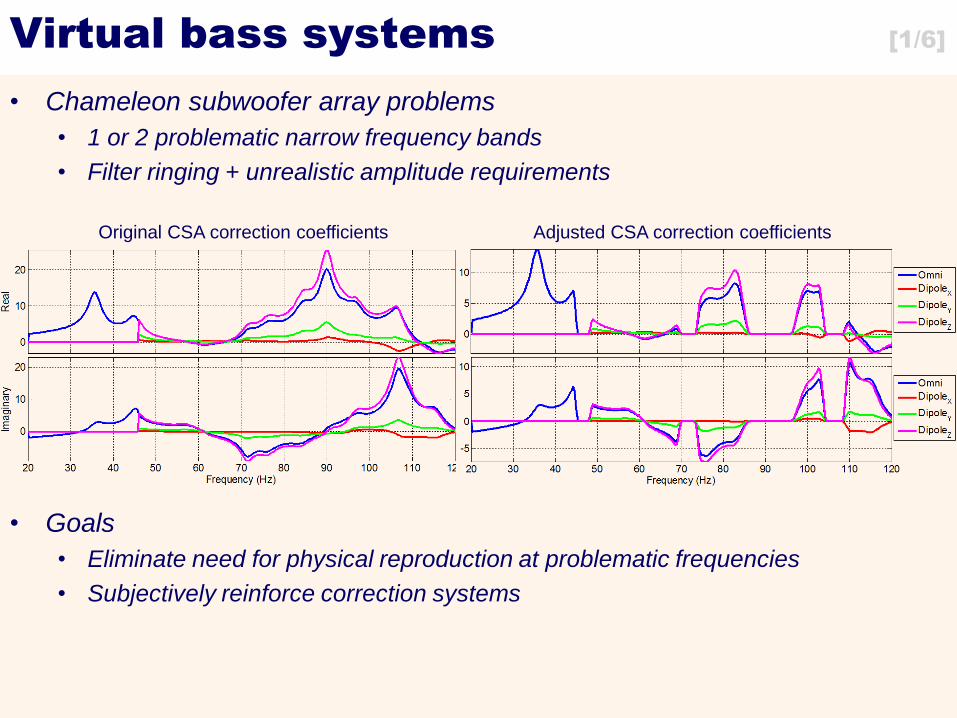
Virtual bass systems [1/6]
• Chameleon subwoofer array problems
• 1 or 2 problematic narrow frequency bands
• Filter ringing + unrealistic amplitude requirements
• Goals
• Eliminate need for physical reproduction at problematic frequencies
• Subjectively reinforce correction systems
Original CSA correction coefficients Adjusted CSA correction coefficients
Virtual bass systems [2/6]
• Principle of the missing fundamental
• Psychoacosutical effect
• Harmonic components = perception of fundamental
• Existing applications
• Loudspeaker/headphone bandwidth extension
• Bass boost
• Implementation approaches
• Time domain
• Frequency domain
• Time/frequency hybrid
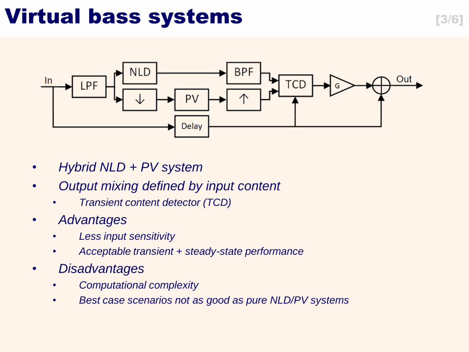
• Hybrid NLD + PV system
• Output mixing defined by input content
• Transient content detector (TCD)
• Advantages
• Less input sensitivity
• Acceptable transient + steady-state performance
• Disadvantages
• Computational complexity
• Best case scenarios not as good as pure NLD/PV systems
Virtual bass systems [3/6]
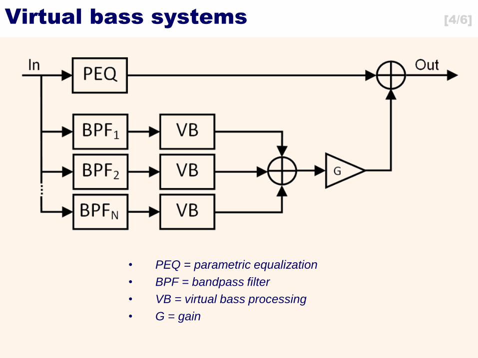
• PEQ = parametric equalization
• BPF = bandpass filter
• VB = virtual bass processing
• G = gain
Virtual bass systems [4/6]
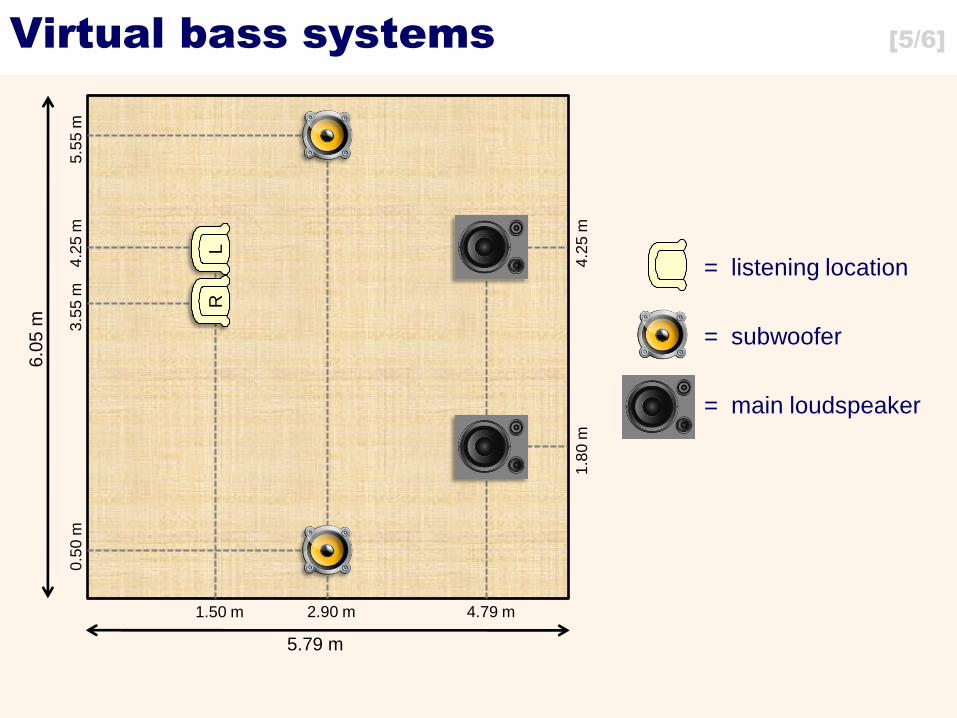
6.0
5 m
5.79 m
1.50 m
3.5
5 m
4
.25
m
4.79 m
1.8
0 m
4
.25
m
5.5
5 m
0
.50
m
2.90 m
L
R
= listening location
= subwoofer
= main loudspeaker
Virtual bass systems [5/6]
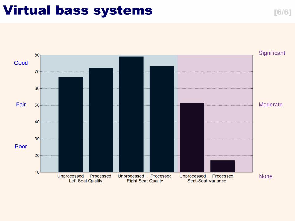
Good
Fair
Poor
Significant
None
Moderate
Virtual bass systems [6/6]
Presentation outline
1. Low-frequency room acoustics
2. Acoustical modeling
3. Simulation toolbox development
4. Conventional low-frequency room correction
5. Chameleon subwoofer arrays (CSA)
6. Virtual bass systems
7. Extended CSA applications
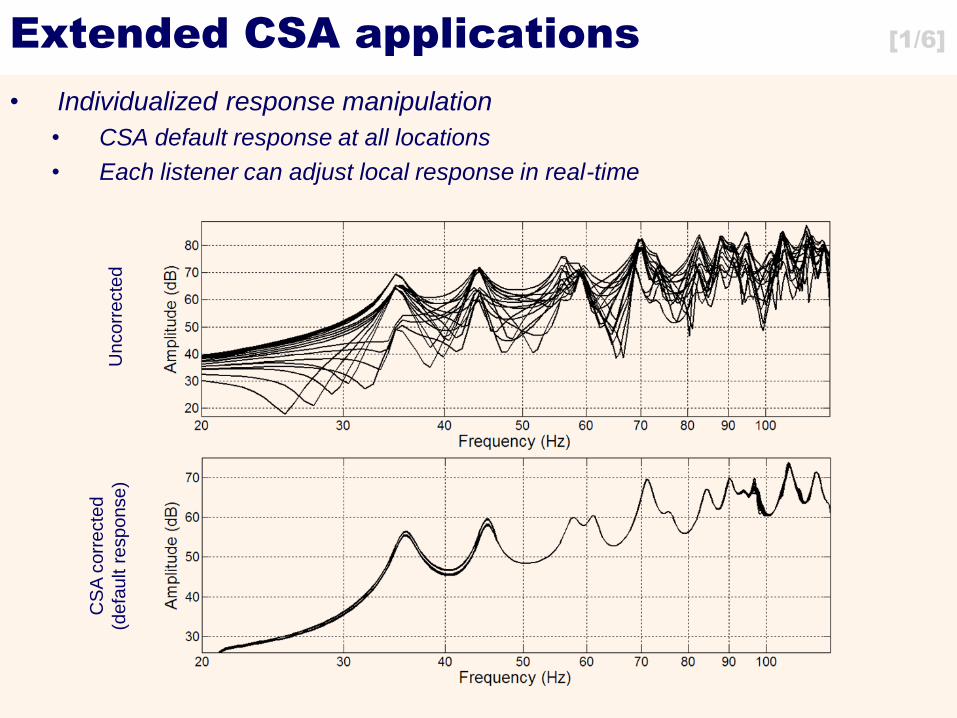
Extended CSA applications [1/6]
• Individualized response manipulation
• CSA default response at all locations
• Each listener can adjust local response in real-time
Uncorr
ecte
d
CS
A c
orr
ecte
d
(defa
ult r
esponse)
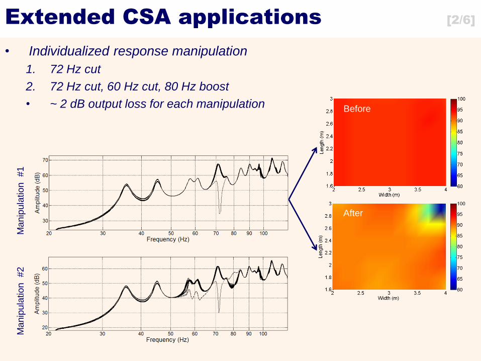
Extended CSA applications [2/6]
• Individualized response manipulation
1. 72 Hz cut
2. 72 Hz cut, 60 Hz cut, 80 Hz boost
• ~ 2 dB output loss for each manipulation
Manip
ula
tion
#1
Manip
ula
tion
#2
Before
After
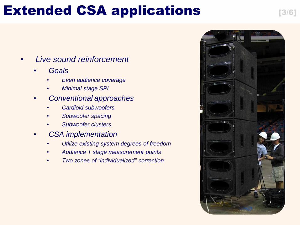
Extended CSA applications [3/6]
• Live sound reinforcement
• Goals
• Even audience coverage
• Minimal stage SPL
• Conventional approaches
• Cardioid subwoofers
• Subwoofer spacing
• Subwoofer clusters
• CSA implementation
• Utilize existing system degrees of freedom
• Audience + stage measurement points
• Two zones of “individualized” correction
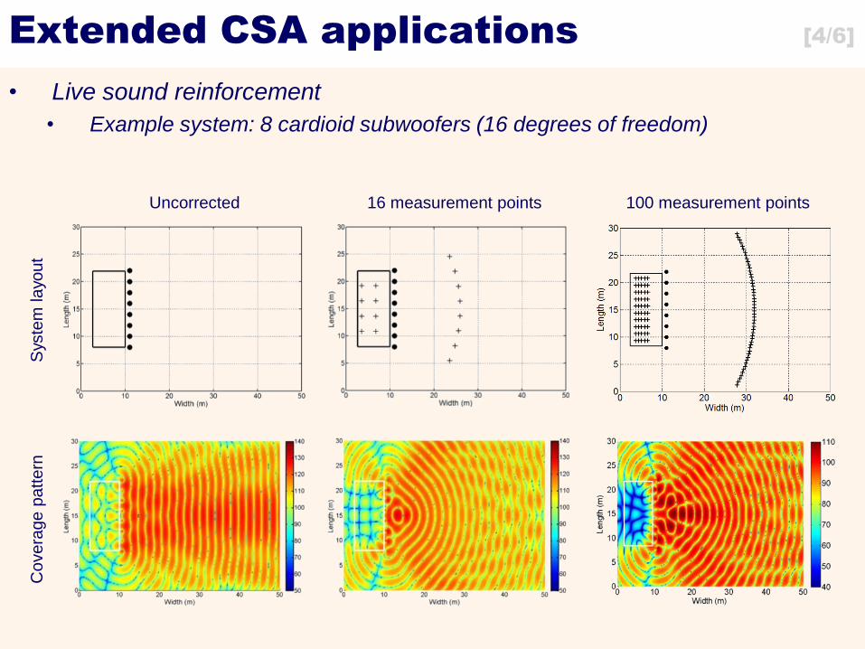
Extended CSA applications [4/6]
• Live sound reinforcement
• Example system: 8 cardioid subwoofers (16 degrees of freedom)
Sys
tem
layo
ut
Covera
ge p
attern
Uncorrected 16 measurement points 100 measurement points
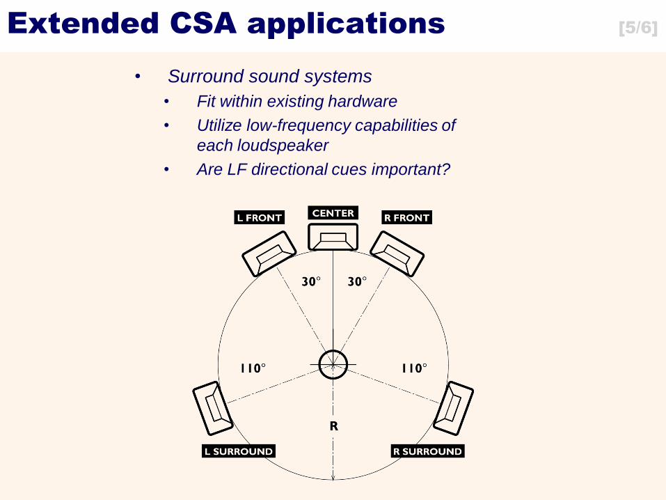
Extended CSA applications [5/6]
• Surround sound systems
• Fit within existing hardware
• Utilize low-frequency capabilities of
each loudspeaker
• Are LF directional cues important?
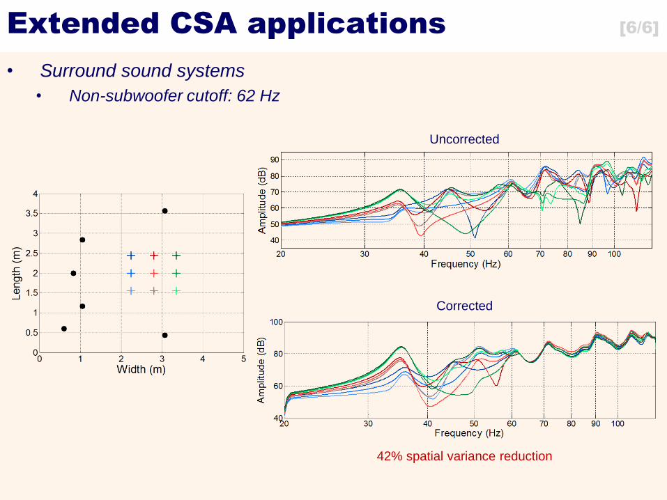
Extended CSA applications [6/6]
• Surround sound systems
• Non-subwoofer cutoff: 62 Hz
Uncorrected
Corrected
42% spatial variance reduction
Conclusions
• Chameleon subwoofer arrays
• Advantages • Minimal spatial variance over wide-area
• Accurate transient response
• Disadvantages • New hardware
• Calibration measurements
• Solutions + alternative implementations
• Virtual bass subjective reinforcement
• Individualized frequency response control
• DSP within surround/live sound systems
Future work
• Hybrid subwoofers
• Drive-unit cross-talk
• Low-frequency extension?
• Chameleon subwoofer array DSP
• Refine window selection procedure
• Problematic filter identification
• System experimentation
Questions?
FDTD + virtual bass software free to download at
www.adamjhill.com