Embed Size (px)
Citation preview

Retrospective Theses and Dissertations Iowa State University Capstones, Theses andDissertations
1996
Chameleon stars: diffusion and spectroscopictransformations in white dwarfsBenjamin T. DehnerIowa State University
Follow this and additional works at: https://lib.dr.iastate.edu/rtd
Part of the Astrophysics and Astronomy Commons
This Dissertation is brought to you for free and open access by the Iowa State University Capstones, Theses and Dissertations at Iowa State UniversityDigital Repository. It has been accepted for inclusion in Retrospective Theses and Dissertations by an authorized administrator of Iowa State UniversityDigital Repository. For more information, please contact [email protected].
Recommended CitationDehner, Benjamin T., "Chameleon stars: diffusion and spectroscopic transformations in white dwarfs " (1996). Retrospective Theses andDissertations. 11142.https://lib.dr.iastate.edu/rtd/11142

INFORMATION TO USERS
Hiis manuscript has been reproduced from the microfilm master. TJMI
films the text directly fi'om the ori^nal or copy submitted. Thus, some
thesis and dissertation copies are in typewriter &ce, while others may be
from any type of computer printer.
The quality of this reproduction is dependent upon the quality of the
copy submitted. Broken or indistinct print, colored or poor quality
illustrations and photographs, print bleedthrough, substandard mar^ns,
and improper alignment can adversely affect reproduction.
In the imlikely event that the author did not send UMI a complete
manuscript and there are missing pages, these will be noted. Also, if
unauthorized copyright material had to be removed, a note will indicate
the deletion.
Oversize materials (e.g., maps, dra\^gs, charts) are reproduced by
sectioning the ori^nal, b^inning at the upper left-hand comer and
continuing from left to right in equal sections with small overlaps. Each
ori^nal is also photographed in one exposure and is included in reduced
form at the back of the book.
Photographs included in the ori^nal manuscript have been reproduced
xerogr^hically in this copy. Hgher quality 6" x 9" black and white
photogr^hic prints are available for any photographs or illustrations
appearing in this copy for an additional charge. Contact UMI directly to
order.
UMI A Bell & Howell Infonnadon Company
300 North Zeeb Road, Ann Aibor MI 48106-1346 USA 313/761-4700 800/521-0600


Chameleon stars: diffusion and spectroscopic transformations
white dwarfs
by
Benjamin T. Dehner
A dissertation submitted to the graduate faculty
in partial fulfillment of the requirements for the degree of
DOCTOR OF PHILOSOPHY
Department: Physics and Astronomy
Major: Astrophysics
Major Professor: Steven D. Kawaler
Iowa State University
Ames, Iowa
1996
Copyright 0 Benjamin T. Dehner, 1996. All rights reserved.

UMI Number; 9626030
Copyright 1996 by De^er, Benjamin T.
All rights reserved.
UMI Microform 9626030 Copyright 1996, by UMI Company. All rights reserved.
This microform edition is protected gainst miauthorized copying under Title 17, United States Code.
UMI 300 North Zeeb Road Ann Arbor, MI 48103

ii
Graduate College Iowa State University
This is to certify that the doctoral dissertation of
Benjamin T. Dehner
has met the requirements of Iowa State University
Major Professor
For the Major Department
For the Graduate College
\
Signature was redacted for privacy.
Signature was redacted for privacy.
Signature was redacted for privacy.
Ill
DEDICATION
To my parents, who made it possible;
and to Susan, who made it worthwhile.

iv
TABLE OF CONTENTS
LIST OF TABLES viii
LIST OF FIGURES ix
ACKNOWLEDGEMENTS x
ABSTRACT xii
CHAPTER 1. WHITE DWARFS: THE CAST OF CHARACTERS 1
1.1 A Historical Perspective 1
1.2 Modern Perspectives and Problems 5
1.2.1 The "DB gap" 5
1.2.2 The coolest white dwarfs 6
1.3 Purpose and Direction of This Work 6
CHAPTER 2. WHITE DWARF EVOLUTION: A LIFE STORY . 8
2.1 Stellar Evolution: A Brief Description 8
2.1.1 The Asymptotic Giant Branch 11
2.1.2 Planetary nebulae 14
2.2 White Dwarfs 15
2.2.1 Masses 15
2.2.2 Spectral classification 16

2.2.3 Pulsations 19
2.2.4 Cooling 20
2.3 Chemical Evolution and Changes in Surface Composition 21
2.3.1 Convection 23
2.3.2 Diffusion 24
2.3.3 Radiative levitation 26
2.3.4 Accretion 27
2.3.5 Mass loss 28
2.4 Things To Come 29
CHAPTER 3. ISUEVO: THE DETECTIVE'S TOOLS 30
3.1 Introduction: Modeling Stellar Evolution 30
3.2 Equations of Stellar Structure 31
3.3 Input Physics 32
3.3.1 Nuclear burning and neutrino emission 33
3.3.2 Opacities 33
3.3.3 Equation of State 34
3.3.4 Convection and mixing 34
3.4 Solving the Equations 36
3.5 Calculation Results: Testing the Code 37
3.6 Summary: What ISUEVO Does 44
CHAPTER 4. ISUEVO II: CALCULATING DIFFUSION IN WHITE
DWARFS 45
4.1 Nomenclature: What is diffusion? 46
4.2 History: A Schatzman Sampler 46

vi
4.3 The Modern View of the Diffusion Equation 48
4.4 Solving the Diffusion Equation 50
4.4.1 Numerical methods 50
4.4.2 Timestep control and the quasi-static assumption 53
4.5 Diffusion Velocities - Representative Results 55
4.6 Physical Explanation of the Diffusion Velocities 57
4.6.1 The driving forces 58
4.6.2 The resistance coefficients 60
4.7 Summary; What Just Happened 67
CHAPTER 5. EVOLUTION RESULTS - TRANSFORMATION
OF THE HELIUM STARS 70
5.1 The Initial Model
5.2 The Diffusion Sequence 72
5.3 Comparing with Observation: Pulsations 77
5.4 Conclusions: the PG 1159 — DB link 82
CHAPTER 6. THE HYDROGEN MODELS 84
6.1 The Initial Model S4
6.2 Evolutionary Behavior 86
6.3 Resolving the Contradiction 88
6.3.1 Ma5s loss 89
6.3.2 Dynamical motions 90
6.3.3 Magnetic fields 90
6.3.4 Radiative levitation 92
6.4 Conclusions 93
Vll
CHAPTER 7. CONCLUSIONS AND SUMMARY: WHERE HAVE
WE COME? 94
7.1 Summary: What has happened 94
7.2 What does it meao? 96
7.3 Where do we go from here? 97
BIBLIOGRAPHY 100
APPENDIX A. SYMBOLS DEFINITIONS 107
APPENDIX B. DIFFUSION SOURCE CODE IDS
B.l Main Diffusion Code 108
B.2 Diffusion Velocity Code 118
B.3 Include File 130

vin
LIST OF TABLES
Table 1.1: Properties of the "first" white dwarfs 4
Table 2.1: White Dwarf Spectral Classifications 16
Table 2.2: PNNi Mass Loss, Pauldrach et al.(1988) 29
Table 4.1: Oxygen Diffusion Velocity Comparison 57
Table 5.1: Evolution of Key Values 74
Table 5.2: Period comparison 80
Table 5.3: Comparison of model characteristics 82
Table 6.1: Hydrogen model evolution - surface abundances by mass . . 88

ix
LIST OF FIGURES
Figure 1.1: HR Diagram, with the main sequence and white dwarfs. ... 3
Figure 2.1: Approximate temperature distribution of white dwarfs .... 17
Figure 3.1: Composition profile of the initial PG 1159 model 40
Figure 3.2: Temperature profile evolution 42
Figure 3.3: Luminosity and central temperature evolution 43
Figure 4.1: Diffusion velocity for PG 1159 model 56
Figure 4.2: Diffusion driving for PG 1159 model 61
Figure 4.3: Surface diffusion driving for PG 1159 model 62
Figure 4.4: Resistance coefficients for a PG 1159 model 68
Figure 5.1: Helium composition evolution 73
Figure 5.2: Helium diffusion velocity evolution 75
Figure 5.3: Mean molecular weight evolution 76
Figure 5.4: Model grid to observation comparison 79
Figure 5.5: Period spacing comparison 81
Figure 6.1: Hydrogen composition evolution 87
Figure 6.2: Hydrogen diffusion velocities 91

X
ACKNOWLEDGEMENTS
In the time and work it took to get to this point, there are many people who
helped me, both professionally and personally. On the professional side, there are
those who helped educate me, and teach about science and its methods. On the
personal side, there are those who helped me learn that life isn't all about school,
and that there is far more to learn than can be gained by sitting in front of a computer
or in a classroom.
For the professional part, my advisor, Steve, who helped me get started; the NSF,
who paid my salary while I did this. Jim Liebert, who pointed me in a good direction.
Don, who got me started, even though I did something else. Roger Alexander, who's
forgotten more about numerical methods than I know, and gave me lots of help. And
not to forget Bonnie, Eriene, Lori, Eva, Joyce, the only ones in the department who
do any real work.
Personally, there are many, many people I have to thank during my career here
at Iowa State. Jerry Mathews, my first instructor here, who was always a help.
Golbon, who it was a pleasure and honor to know. The clan - Charley, Jeff, Susan
(S.), Ken, Mark, Rich, Steve, Vandy. The slugs - Scott, Anthony (Dad!), Mikey,
Karen, Doug, Kathy, Phil, and Matt. Chuck, Bruce, Kevin, Ralph, the bastards. A
special thanks to Susan K., for, well, being Susan. Max, for getting me started on

xi
mystic; Athen, for getting me started on netrek. Don, for being that humble and
modest sort of guy he is, and for showing me how to golf. Can't forget to mention
the group - Doug, Andy, Dan (the originals), Paul, Kurt (in spirit, anyway), Curt,
Brian (once or twice,) John, Theresa, Jim, Ginger, Kari, and Jennifer.
Life is a crap sandwhich -
the more bread you got, the less crap you gotta take
- Tom Servo

Xll
ABSTRACT
White dwarfs stars are the end product of stellar evolution, generating no energy
by nuclear fusion, slowly cooling over time. As they cool, their intense gravity causes
the lightest element - either hydrogen or helium - to float to the surface. This "grav
itational settling" is responsible for the observed nearly pure surface composition of
white dwarfs. In this investigation, I model this settling process in these stars by
constructing a sequence of models which represent the star at different stages as it
cools.
As white dwarfs cool, at certain temperatures they undergo nonradiai pulsations.
Most importantly, a change in the composition as a function of the depth within the
star causes differences in the pulsations of the star. Pulsations are then a natural way
of measuring the depth of surface layers of pure composition formed by gravitational
settling.
I calculated a sequence of models representing the evolution of white dwarfs.
The initial model was of a young, hot white dwarf at a surface temperature of Tetr ~
130,000K, representing the pulsating white dwarf PG 1159. The model has a surface
layer of mixed He, C, and 0 containing about 10"^ of the stellar mass. This model
weis evolved until it cooled to 25,000K, where it again undergoes pulsations. By this
temperature, settling causes the formation of a surface layer of helium containing

about 10~® of the stellar mass. Observations of GD 358, a pulsating helium-rich
white dwarf at Tes ~ 25, OOOA', show that it has a surface helium layer of roughly
this thickness. This indicates that stars like PG 1159 may evolve to stars like GD 358,
despite the incongruity in surface layer mass.
Finally, there exists a range of temperature, from 45,000K to 30,000K, where
all observed white dwarfs have hydrogen dominated surfaces. I added hydrogen to
the PG 1159 models to investigate its effects. The calculations show that hydrogen
diffuses very quickly to the surface, and would be present at the surface in detectable
quantities. This contradiction with observations of PG 1159, which shows no de
tectable hydrogen, implies some other mechanism, such as mass loss, which alters
the surface abundance of white dwarfs.
1
CHAPTER 1. WHITE DWARFS: THE CAST OF CHARACTERS
Strange objects which persist in showing a type of spectrum utterly out of
keeping with their luminosity may ultimately teach us more than a host
which radiate according to the rule.
A. Eddington (1922)
This dissertation concerns the modeling of the evolution of white dwarf stars.
However, before addressing what is to be done, it is even more important to ask why
it is to be done at all. What broader questions exist, and where, in the framework
of astronomy, does this work fit in? First, therefore, I start with the history of white
dwarf stars, and the solution to the initial puzzle posed by their very existence. I
then give a modern perspective on the role of white dwarfs in contemporary stellar
astrophysics. Finally, I preview the work presented in this dissertation, and how it
fits into this framework.
1.1 A Historical Perspective
In the quote at the beginning of this Chapter, Eddington was referring to the
then recently discovered class of white dwarf stars. The debut of this strange class of
faint stars was in 1783, when 40 Eri B was "discovered" by William Herschel (Her-
schel, 1783, 1785). This wcis followed by the discovery of Sirius B in 1862 by Clark
2
(Bond 1862). Though known to be underluminous for their mass in comparison with
normal stars, they were not thought to be otherwise unusual until spectroscopic mea
surements were made early in the twentieth century. They were then both classified
as spectral type A, i.e., hotter than the Sun, with the observations of 40 Eri B in 1910
(Hertzsprung 1915), aind Sirius B in 1914 (Adams 1915). This presented a mystery,
since simple radiative theory indicates that such hot stars must be faint because of
very small size - nearly the size of the Earth. This, in turn implies a mean density
of over 100,000 times greater than the Sun!
Some of the properties of these first white dwarfs and their companions are
summarized in Table 1.1,^ which gives the effective (surface) temperature Teff, the
mass and luminosity in solar units, M© and L©, and the distance in parsecs from the
Sun. As can be seen, the white dwarf stars are very low luminosity, but have masses
similar to the Sun and a much higher temperature.
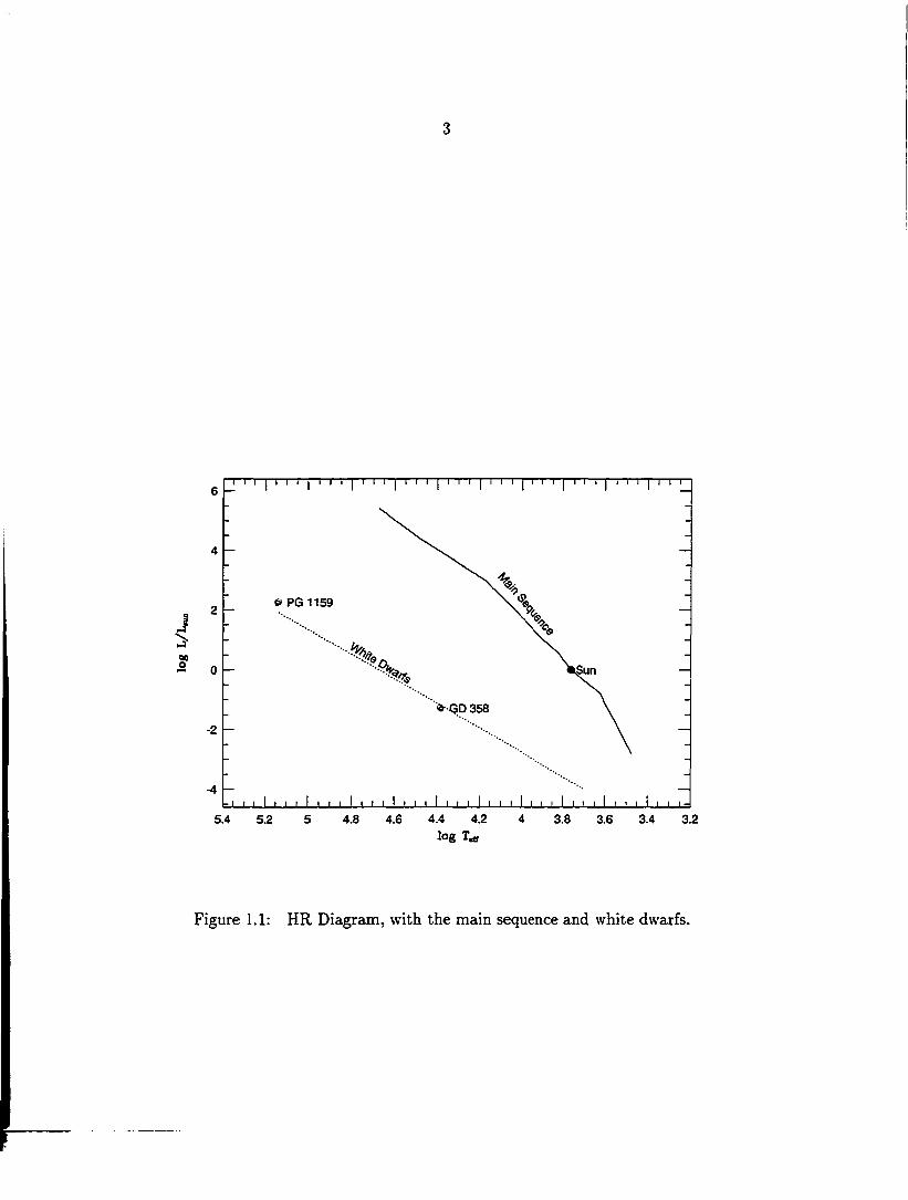
The numbers given in Table 1.1 are shown more graphically in Figure 1.1,^
which shows the location of the main sequence of hydrogen burning stars and the
white dwarfs. The location of two special stars - PG 1159-0.35 and GD 358 - are
also marked in this diagram. These stars play an important role in my investigation.
An understanding of the internal structure of white dwarfs developed in 1926
when R. Fowler speculated that the interiors of white dwarfs were governed by the
(then novel) Fermi-Dirac statistics (Fowler 1926). He speculated that the central
support of the star against gravity came from electron degeneracy pressure. This idea
^Data on the white dwarfs taken from McCook & Sion (1987), and data on the main sequence stars from Hoffleit (1982)
^Main sequence data taken from Bowers k. Deeming (1984) Table 3.1 while the white dwarf data is from stellar models used in this investigation.
3
e PG 1159
iSun
4.2 4.6 4.4 4 3.8 3.4 3.2 5.4 5 4.8 3.6 5.2 log
Figure 1.1: HR Diagram, with the main sequence and white dwarfs.

4
Table 1.1: Properties of the "first" white dwarfs
Star mv L ( L e ) Teff(K) M ( M 0 ) Distance (parsecs)
4 0 Eri A 4.5 0.3 5,080 0.75 4.8 40 Eri B 9.7 0.0027 12,700 0.44
Sirius A -1.5 23.0 9,130 2.35 2.6 Sirius B 8.3 0.002 25,400 0.98
was further elaborated upon in 1939 by S. Chandrasekhar who further demonstrated
that white dwarfs could never exceed approximately 1.4M@ in mass; this weis the
largest mass that could be supported by electron degeneracy pressure (Chandrasekhar
1939).
As more white dwarfs were discovered, it was found that nearly all had pure
elemental surface composition, with that surface being either hydrogen or helium. In
the early 1950's, Evry Schatzman showed that this purity results from gravitational
settling; heavier elements sink to the center of the star, and the lightest elements
float to the surface (Schatzman, 1958). However, it still remained a mystery as to
why some retained hydrogen at their surface while others did not. .A.nd, further, the
question of the origins of white dwarfs remained unanswered.
Schatzman (1958) and Schwarzchild (1958) both speculated that the degenerate
configuration of white dwarfs may follow the exhaustion of all available nuclear fuel.
A main sequence star supports itself against gravity by generating energy through
nuclear fusion, and so perhaps, they argued, when a star runs out of fuel, it would
collapse into the degenerate configuration of a white dwarf. While this is correct
in a broad sense, we now know that the true path that a star take to becoming a

white dwarf is much more convoluted, as will be discussed in more detail in the next
Chapter.
1.2 Modern Perspectives and Problems
Two fundamental cispects of white dwarfs have direct bearing on this investiga
tion. First, white dwarfs come in two major "flavors", with either helium or hydrogen
dominated surfaces. The origins of this dichotomy are still not well understood. Sec
ond, white dwarfs have been established as the end stage of stellar evolution for stars
between 0.8 and 8 times the mass of the Sun (see Chapter 2 for details.) This implies
that the properties of both individual white dwarfs and the aggregate properties of
the population place some conditions on their predecessor stars. In particular, the
white dwarf population contains a history of star formation in the galaxy, and so un
derstanding white dwarf evolution is a link to understanding galactic star formation,
as shown by, for example. Wood (1992).
1.2.1 The "DB gap"
As stated, white dwarfs usually have either pure H or pure He surface layers.
This dichotomy is the basis of the spectroscopic classification now in use for these
stars. The three main categories are the DA stars, with surfaces rich in hydrogen;
the DB stars, which show neutrcil helium (He I) surface features; and the DO stars,
which show ionized helium (He H) surfaces. While white dwarfs have a wide range
of surface temperatures, from ^ 100,000K down to ~5000K, there are no helium-rich
white dwarfs between 45,OOOK and 30,000K, as described by Liebert (1986). HeHum
rich stars are found at temperatures both above and below this gap, however. Given
6
that white dwarfs generate no energy, and therefore must cool, one must ask "Where
are the helium white dwarfs between 45,000K and SOjOOOK?" This "DB Gap" implies
that there must be some mechanisms or processes that hide the surface helium at
45,OOOK and re-introduce it at 30,000K in some white dwarfs, such as discussed by
Liebert, Fontaine, & Wesemael (1987).
1.2.2 The coolest white dwarfs
As the ultimate remnants of most normal stars, white dwarfs can provide an
archaeological record of the history of star formation in the galaxy. Most importantly,
as the coolest white dwarfs are the oldest objects in the galactic disk, identification
of the low luminosity white dwarfs provides a time limit on star formation in the
galaxy. This facet of white dwarfs has been explored extensively following the work
of Winget et al.(1987); see for example Iben & Laughlin (1989) and Wood (1992).
Obviously, there are uncertainties inherent in this approach; despite these difficulties,
Liebert et al.(198S), using data from several surveys, have determined that there
are essentially no white dwarfs fainter than ~0.00003 solar luminosities. Models of
cooling white dwarfs by Wood (1992) which match the luminosity function cutoff
have indicated an age for the galactic disk of 8 to 10 Gyr. This range reflects our
remaining uncertainties about white dwarf structure, the principle one being the
surface compositional structure.
1.3 Purpose and Direction of This Work
The goal of this dissertation is to examine the diffusive processes that alter the
surface layer composition during white dwarf evolution. Diffusion may play a role

7
in producing the observed phenomenon of the DB gap, as well in determining evolu
tionary links between various types of white dwarfs. Most of the work on diffusion
in white dwarfs over the past four decades has focused on specific phenomena of
white dwarf atmospheres. However, only a very few comprehensive computations of
white dwarf evolution incorporating time-dependent diffusion have been done, and
none have been made since the remarkable results that have come from the studies
of the pulsating white dwarfs. In this work, I construct white dwarf evolutionary
sequences that include time-dependent diffusion and compare them directly with the
new observations.
In the next Chapter, I will review the modern view of white dwarf origin and
evolution. In chapter 3,1 discuss the evolution code and the numerical methods used
to solve the equations governing white dwarf structure and evolution, and in Chapter
4 I elaborate on the treatment of diffusion used in the evolution code. Chapter
5 describes the results for helium-rich surface models, and Chapter 6 explores the
behavior of hydrogen-rich models. In Chapter 7,1 summarize the results and examine
the accomplishments of this investigation.

8
CHAPTER 2. WHITE DWARF EVOLUTION: A LIFE STORY
What is their history? What their destiny? What their function in the
universal scheme of things?
- Agnes M. Gierke (1903)
In this Chapter, I will review some of the conventional idea^ of stellar evolution,
concentrating on the formation of white dwajfs. This review provides the background
against which the investigation presented in the following chapters was conducted.
Further, I wish to pose some of the questions and point out uncertainties in current
thinking; these are the motivation for this investigation. Finally, I will also discuss
how the properties of observed white dwarfs may be related to their progenitor stars.
2.1 Stellar Evolution: A Brief Description
An anonymous astronomer once quipped "A star is nature's way of making
a white dwarf." This is at best an oversimplification of stellar evolution and white
dwarf formation, although it is relevant to the description of evolution in this Chapter.
Most, but not all, stars will become white dwarfs. For stars which do become white
dwarfs, there may be several possible evolutionary paths to that end. Some general
introduction to stellar evolution is available in such texts as Clayton (1983) and
Hansen & Kawaler (1994). Here, I will focus on those stars which become white

9
dwarfs, and, on what appears to be the most common paths they take. Some excellent
reviews, on which this chapter is based, can be found in Iben Sz Renzini (1983, 1984),
and Iben & Tutukov (1984).
The story of evolution is an account of the conflict within a star of internal
pressure against gravitational collapse. For most of a star's life, while it is on the main
sequence, the nuclear fires in the core of the star convert hydrogen into helium and
energy, heating the core and providing long-term support against gravity. Eventually,
though, the hydrogen fuel becomes exhausted; the evolutionary path taken by the
star at this point depends on the mass.
When the core of the star runs out of hydrogen, the (now helium) core begins
to contract, and hydrogen fusion continues in a shell surrounding the core. This is
accompanied by expansion and cooling of the star; this maintains and then increases
its luminosity as the shell thins. The star is now a "red giant", and, with its changed
state, ha^ ascended the "red giant branch" (RGB). Along with the ascent of the red
giant branch comes the "first dredge-up." A convection zone forms, which reaches
down from the outer layers to convectively mix underlying material which has un
dergone nuclear processing. The results of this dredge-up are discussed by Becker &
Iben (1979) and summarized by Iben &: Renzini (1984).
For stars greater than about 3 M©, the helium core will begin to undergo fusion
quiescently. This helium core-burning star will descend the red giant track, and begin
to burn helium in the core at higher temperatures and lower luminosities along helium
burning loops, as shown in Iben & Renzini (1984).
The cores of stars less massive than 2-3 Mq, however, do not have the internal
pressure to ignite helium fusion at moderate densities; instead, these stars will develop

10
a electron degenerate helium core, where the gravitational pressure is balanced by
the quantum mechanical interaction of the closely packed electrons. In this state, the
pressure exerted by the electrons depends only on the density, and is independent of
the temperature.
Eventually, these degenerate cores reach a sufficiently high temperature to be
gin helium fusion in a "helium flash". The fusing helium releases energy and heats
up the core, but the increased temperature does not affect the pressure, due to the
degeneracy. The temperature increase does, however, increase the energy generation
rate, thus further raising the temperature. This runaway cycle continues until the
temperature in the core is high enough to remove the degeneracy condition. Given
that this helium flash can happen on a timescale of minutes, as shown by the cal
culations of Cole & Dupree (1980, 1981), it is somewhat of a mystery that the star
as a whole does not explode. However, such stars do not catastrophically explode,
since low mass stars, which must have undergone a helium flash, are observed quietly
burning helium in their cores as horizontal branch stars in globular clusters.
Finally, regardless of the ignition conditions, the following stages occur when
the helium fuel in the core becomes exhausted. Similar to the earlier stage, where a
shell burning hydrogen source ignited, a helium-burning shell surround the carbon-
oxygen core. The star expands and cools in a manner similar to the first ascent of
the red giant branch, and ascends the «isymptotic giant branch (AGB). As it ascends
the AGB, the surface convection zone deepens in star, contributing to the "second
dredge up."
High mass stars may then ignite carbon in their cores, and continue with nuclear
reaction with elements of increasing atomic number. These stars typically continue

11
until producing iron in their core; at this point, these stars can undergo a supernova
explosion. These high mass (> 9M©) stars are beyond the scope of this dissertation.
I focus on less massive objects which have a less catastrophic end to their lives.
2.1.1 The Asymptotic Giant Branch
The asymptotic giant branch (AGB) represents the final throes of a dying star.
One of the most important processes in this phase of the stars life (or death) is that
the star may lose much of its mass during this time. As discussed by Weidemann
(1990), it has become increasingly apparent that stars of up to 9 (possibly more) M©
are the predecessors of white dwarf stars, which must be less than the Chandrasekhar
limit of 1.4M0.
Models by Bowen & Willson (1991) demonstrate how mass loss driven by large-
amplitude pulsation on the AGB leads to the inevitable formation of a "superwind".
Their models show how the superwind may naturally increcise to very large values,
thus terminating the AGB.
AGB evolution is naturally divided into two periods, the "early AGB" (E-.4GB)
and the "thermally pulsing AGB" (TP-AGB); see, for example, Iben & Renzini (1983)
& Iben (1991). During the early part of a star's life on the AGB, it derives most of its
luminosity from an outer hydrogen burning shell. However, as the hydrogen burns,
it deposits the resultant helium "cish" in a shell beneath it. Eventually, this helium
ash reaches high enough density to ignite at its bcise, where it is mildly degenerate,
in an event referred to as a thermal pulse. When the helium shell undergoes fu
sion, the energy generated causes it to expand, pushing out the outer hydrogen shell
and extinguishes hydrogen burning. The helium shell deposits its carbon ash onto
12
the growing degenerate core. Eventually, the helium burning subsides by expansion
and cooling, followed by re-ignition of the hydrogen-burning shell in the subsequent
relaxation. These episodes of helium burning add mass to the carbon/oxygen core.
The luminosity of a star with a degenerate carbon/oxygen core and a hydrogen
shell source, i.e., on the AGB, is determined primarily from the mass of the core, and
is independent of the envelope. As originally demonstrated by Paczynski (1970), the
AGB luminosity is given by
where Mc is the mass of the degenerate core. This "core m«Lss-luminosity relation"
holds for all but the most luminous AGB stars, as discussed by (for example) Blocker
k. Schonberner (1991). Hence on the AGB the star's position in the H-R diagram
is determined by the core mass, and not the total mass, and the evolution of the
core and envelope are to a large extent decoupled. However, once the AGB star
has lost enough mass, it leaves the AGB to regions of higher temperatures as the
hot core becomes exposed. Most white dwarf stars are assumed to form from such
"post-AGB" objects, which have ascended the AGB, and then moved off of the AGB
to regions of higher temperature, losing most of their outer envelope. The models of
Paczynski (1970), Iben & Tutukov (1984) and Schonberner (1983) show how post-
AGB evolution can lead to the development of the white dwarfs through this channel.
There is another channel into the white dwarf cooling track for stars in which the
envelope is not massive enough to ascend the AGB. Such objects instead evolve to
white dwarfs through the subdwarf (sd) phase. Vauclair and Liebert (19S7) discuss
this scenario in the context of white dwarf formation, while models by Dorman, Rood
& O'Connell (1993) and others display evolutionary tracks. This channel into the
(2.1)

13
white dwarf region produces white dwarfs at the low-mass end of the distribution
(between 0.50 and 0.55 M©) and is not thought to be a major contributor to the
total white dwarf population. Hence, these objects will not be considered here. I will
instead concentrate on stars which proceed through the thermally-pulsing AGB to a
possible planetary nebula nuclei (PNNi) stage, where they then cool (possibly as a
"PG 1159" star) before settling on the white dwarf cooling track.
As an AGB star loses mass the luminosity increases and the mass loss rate
increases. Initially, the effect of the mass loss on T and L is small; see the models of
Bowen & Willson (1993). However, as discussed by Paczynski (1970) and Schonberner
(1983), when the envelope is thin enough due to mass loss, at about lO'^Me, the
effective temperature strongly depends on the remaining envelope mass. Essentially,
as long as the envelope is thick enough, the core is hidden from view. However, as the
envelope further thins, the inner core becomes exposed and the effective temperature
of the star increases dramatically.
If a star leaves the AGB during a thermal pulse, then the extended envelope -
with the remnant hydrogen - can be entirely lost, implying this newly formed star
will have a helium rich surface. If, however, the star leaves the AGB during the
hydrogen burning phase, it will still retain a hydrogen rich surface. Iben (1984) notes
that an AGB model spends about 80% of its lifetime in the hydrogen burning phase,
so, therefore, approximately 80% of the white dwarfs formed as post-AGB object
should be hydrogen rich white dwarfs. This scenario implies that a white dwarf is
"born" as either a hydrogen-rich (DA) white dwarf, or a helium-rich (DB/DO) white
dwarf, and thereafter remains that way.

14
2.1.2 Planetaxy nebulae
Whether or not a proto-white dwarf will form a planetary nebula depends on the
competition between the mass loss rate and the evolution rate of the star. During
this stage of evolution, the star becomes hotter, as the outer envelope is lost and
more of the hotter core is exposed. As the outer envelope expands to the radius
of a planetary nebula, the star must be hot enough (Teff ~30,000K) to ionize the
material to form the nebula. If the star evolves to higher temperatures too slowly,
the expanding material will expand and disperse before it can become ionized by
the central star. The age of a planetary nebula can be estimated by measuring
the size and the expansion velocity of the nebula; these dynamical ages consistently
disagree with the theoretical models. This disagreement between the observationally
determined ages of planetary nebulae and the theoretical ages is discussed by Gathier
& Pottasch (1989).
A recent explanation for this has been forwarded by Blocker (1995). He demon
strates that the cooling timescale is also dependent on the initial mass of the object
while it is on the AGB. A more massive object will have a higher internal tempera
ture, and will have a less degenerate core. This lesser degree of degeneracy in turn
leads to a shorter cooling timescale than would otherwise be expected.
At the core of a planetary nebula is an object referred to, obviously enough, as a
"planetary nebula nucleus", or PNN (plural = PNNi). (Sometimes these are referred
to as "central stars of planetary nebulae", or CSPN, or, occasionally, "central stars".)
Gathier & Pottasch (1989) discuss some of the properties of PNNi; these objects
typically have a surface gravity somewhat less then the white dwarfs, with log^r ~ 6,
and have temperature ranging from roughly 30,000K to over 100,000K. These objects

15
are often considered intermediates between white dwarfs and the AGB.
2.2 White Dwarfs
In the iirst Chapter, white dwarfs were introduced as being very small, hot
stars, maintaining themselves against gravitational collapse with electron degeneracy
pressure. Now I will go into more detail about their structure, and properties as a
class.
2.2.1 Masses
The "typical" white dwarf is an object about the mass of the sun and the size of
the earth. As reviewed by Weidemann (1990), white dwarfs have a strong uniformity
in mass, with the bulk of them being at or near 0.6 M©. For a sample of 126 hydrogen-
rich white dwarfs, Bergeron, SafFer, and Liebert (1992) determine a mean mass of 0.56
M©, with a standard deviation of 0.137 M©. The distribution is more sharply peaked
than a Gaussian, with a tail extending to the high mass end. Their mean surface
gravity is determined to be log^ = 8.0, which implies a radius of approximately lO"'^
times that of the sun, or about the size of the Earth.
This strong uniformity in white dwarf masses is itself curious. Since white dwarf
predecessors on the main sequence may be cis large as 9 M©, this is indicative of the
amount of mass that these stars must somehow loose on the way to becoming a white
dwarf. The narrowness of this distribution can be understood, at least qualitatively,
as resulting from the feedback between the Paczynski (1970) core mziss-luminosity
relation and the steep luminosity dependence of the Bowen & Willson (1993) mass
loss description (e.g. Kawaler 1996.) This convergence of evolutionary paths of white

16
dwarfs simplifies their modeling in certain respects, though it complicates their use
as archcieological specimens.
2.2.2 Spectral classification
The spectral classification for white dwarf stars as described by Sion (1986),
which is summarized here. Also included are the variable white dwarf types not
considered by Sion (1986). The basic properties and classification scheme is given in
Table 2.1.
Table 2.1: White Dwarf Spectral Classifications
Type (K) features DA < 80,000 H lines DB < .30,000 Hel lines DO >47,000 Hell or Hell lines DC <5000 no lines DQ <10,000 carbon DZ anywhere metals
DAV (ZZ Ceti) 10,000-13,000K pulsation DBV (GD 358) 20,000K - 27,000K n
DOV (GW Vir) >80,000
A graphical representation of Table 2.1 is shown in Figure 2.1, with the tem
perature regions inhabited by each variety of white dwarf indicated. The pulsational
instability strips of variable stars are also noted. One may be tempted to think of the
stars in the diagram as "evolving" from left to right, as they cool. While essentially
correct, this simple picture may easily mislead; white dwarf evolution will be more
fully discussed in the next Section.
The DA stars have a surface rich in hydrogen, with an apparently pure surface

17
GWVir (DOV)
ZZCeti (DAV)
j i DA
DO
Central Stars
I
GO 358 (DBV)
DB Gap -DB-
DZ
DQ
1.6x10° 1.2x10 80000 Surface Temperature (K)
40000
Figure 2.1: Approximate temperature distribution of white dwarfs

18
hydrogen layer (H/He < 10"'^.) The hottest known DA stars are at about 80,000K,
while the coolest DAs are at about 6000K. Above 80,000K it is believed that hydrogen
will be completely ionized, and thus spectroscopically invisible; likewise, below 5500K,
hydrogen becomes spectroscopically invisible as well. The effective temperature range
from roughly 12,230K to 10,300K, as determined by Kepler & Nelan (1993), is known
as the ZZ Ceti instability strip, where almost all observed DAs pulsate. A few non-
pulsating DAs have been found in this region as well by Kepler & Nelan (1993), which
leads Kepler (1995) to speculate that the location of the instability strip may be meiss
dependent; this mass-dependence would require that higher mass stars pulsate within
a higher temperature range.
The DB stars, which show lines of neutral helium, are found at Tesr between
30,OOOK and r2,000K, below which the helium lines disappear. Though such stars
would easily be identifiable as DB white dwarfs, there are no helium-rich white dwarfs
in the range between 30,000K and 45,000K; this is called the "DB gap", and will
discussed in the next Section. Between approximately 20,000K to 28,000K (Thejll et
al.l991) are found the pulsating DB stars, with the prototype being GD 358.
The DO stars, distinguished by the presence of He II lines, are among the
hottest known white dwarfs, with temperatures as high as 180,000K down to roughly
47,OOOK. Some DO stars show evidence for large abundances of carbon and oxygen;
these stars are known as the PG 1159 stars after their prototype. Some PG 1159 stars
are also pulsating stars — the "GW Vir" stars, of which PG 1159 is again the pro
totype. The exact boundaries of the GW Vir instability region in the H-R diagram
are uncertain due to large uncertainties in the surface temperatures of these stars.
Atmospheric models by Werner et al.(1991a) indicate that if hydrogen is present in

19
the atmospheres of the DO stars, it must be at an abundance of less than 5% by
mass.
The PG 1159 stars are often considered proto-white dwarfs, stars starting to
maJke their way down the white dwarf cooling tracks. These stars are characterized
by high surface temperatures (> 100,OOOK), strong metal abundances (mostly C,
N, &: 0), and no detectable hydrogen. Given the above classification scheme, these
stars could be classed as DOZQ stars. These objects are believed to be intermedi
ate between the PNNi and the hot DO white dwarfs. Whether or not they are a
link between the AGB and all white dwarf stars is still a somewhat open question;
the answer depends on whether or not enough hydrogen remains in these stars to
eventually turn them into DA stars.
Dreizler et al.(1995) discuss observations of "hybrid PG 1159" stars, which show
spectra characteristic of the PG 1159 stars, except that these hybrid objects clearly
show the presence of hydrogen. These stars appear to be to located midway between
the PG 1159 stars and hot DO stars on the H-R diagram, but as yet few of these
(three) have been discovered.
2.2.3 Pulsations
As seen in Table 2.1, some white dwarfs pulsate. These pulsating stars are
extremely important, both in the general sense and in this investigation, because the
pulsations are a probe into the interior structure of the star. The study of pulsating
white dwarf stars has made many advances in recent years, due in large part to the
advent of pulsational studies with the Whole Earth Telescope (WET), described by
Nather et al. (1990). These studies allow a direct probe into the internal structure of

20
these objects, giving a solid observational foundation for structural and evolutionary
models.
The location of the instability regions in the HR diagram are a matter of great
debate. Temperature estimates are derived from comparison of observation with at
mospheric models, with uncertainties of roughly several hundred degrees, and more
for the DBV and DOV stars. Further, systematic uncertainties, such as errors in the
the input physics of the models, can raise this substantially. Theoretical estimates of
the location of the instability regions, i.e., from evolutionary models, depend heav
ily on tissumptions made about convection within the star, such as the convective
efficiency; see, for example, Tassoul et al.(1990.) A more precise temperature deter
mination would perhaps be a useful way to calibrate models of convection.
Paradoxically, while this dissertation is concerned with chemical evolution, spec
troscopy plays a very small part, since the spectroscopic differentiation between "pure
hydrogen" and "pure helium" does not require sophisticated spectroscopic meaisure-
ments. (Not, at least, at the temperatures of the objects in this dissertation.) On
the other hand, while this is not a study of variable stars, stellar pulsations play a
key role in this study, since these pulsations provide an essential probe of the internal
structure of the star.
2.2.4 Cooling
Many of the aspects of white dwarf cooling are summarized in the review by
D'Antona & Mazzitelli (1990). A white dwarf can well be described as "a hot brick
surrounded by a blanket", a hot central core slowly losing energy through a sur
rounding insulating envelope. This basic model of a cooling white dwarf was first
21
introduced by Mestel (1952), in which he assumed a degenerate isothermal core (the
brick) which cooled by radiative diffusion through a surrounding non-degenerate en
velope (the blanket.) While this model neglects some of the relevant physics, it is
still a good approximation to the cooling of white dwarfs.
Early in a white dwarf's cooling history, neutrino emission becomes an important
mechanism for the star's cooling. As shown by Iben & Tutukov (1984), models of
very young, hot white dwarfs at luminosities between 1.5 > log(L.y/L0) > 0, have a
neutrino luminosity which exceeds the photon luminosity. Kawaler et al.(1985) show
that higher mass white dwarfs should have a much more significant neutrino cooling
over a larger range of luminosities. In general, neutrino cooling causes the cooling
timescale to be faster than the classical Mestel time.
Lamb k Van Horn (1974), Iben &: Tutukov (1984) and Wood (1992) also show
that later in the white dwarf's life, when log(X/L©) ~ —3, other effects such as
crystallization of the core, and Debye effects (a quantum mechanical effect which
causes a decreased specific heat) will occur. When the core begins to crystallize,
this will release latent energy from the interior, thus slowing the cooling of the white
dwarf. After this, however, the now crystalline interior will have a lower specific heat
then gaseous phase, and will tend to cool more quickly. While the details of white
dwarf cooling are actively being investigated, this basic picture is clear.
2.3 Chemic£d Evolution and Changes in Surface Composition
The processes controlling the chemical evolution of white dwarfs are complex.
As seen in Table 2.1 and Figure 2.1 there is a temperature range between roughly
45,000K down to 30,OOOK where there are no observed helium rich white dwarfs.

This phenomena, called the "DB gap" has been noted by Wesemael et al.(19So) and
Liebert (1986). That this gap exists at all indicates that some dynamical mechanism
must operate in at the hot helium-rich star which can change the surface composition.
Liebert et al.(1987) suggest that the blue (high temperature) edge of the gap is caused
by gravitational settling, which causes hydrogen to float to the surface of the star
covering the helium as the star cools to 45,000K. Subsurface convection zones, which
form at about 30,000K, reach from the hydrogen surface into the deeper helium layers,
then mix the helium back to the surface to account for the red edge. While plausible,
this scenario has yet to be demonstrated to occur in evolutionary models.
The red edge of the gap is defined by the star PG 0112+104, the hottest known
DB below the gap. The temperature of this star is somewhat uncertain; several
results are summarized by Thejll et al.(1991). While all results consistently list this
star as the hottest DB below the gap, there is a discrepancy between the results of
different researchers. The currently "accepted" value for the temperature of this star,
by Thejll et al.(1991) is 27,000K ± 2000K.
Sion (1986) discusses a possible two-track evolutionary scheme for white dwarfs,
supposing that DAs and DBs evolve along separate evolutionary tracks. Further, Sion
speculates that there are possible tracks by which one type may change to another,
consistent with the presence of the DB gap. This discussion by Sion points out many
questions and uncertainties which are at the heart of current investigations in white
dwarf evolution.
Further, the PG 1159 stars could be the precursors of all white dwarfs, if one can
explain the transition from the metal-rich PG 1159 surface composition to the much
more chemically pure DA and DB stars. At cooler temperatures, there is the high

23
metal abundances in the DQ and DZ stars. As noted by Sion (1984), the temperature-
dependent distribution of these objects is additional evidence for the existence of some
mechanism (or mechanisms) which can alter the surface abundance.
To model white dwarf chemical evolution correctly, there are five mechanisms
which much be considered: mass loss, diffusion, convection, radiative levitation, and
accretion of interstellar material. Each of these plays a significant role at one time or
another in the "life" of a white dwarf. In this dissertation, while I focus on diffusion,
I also address each of the others to see what insight my models may give concerning
the importance of these mechanisms.
2.3.1 Convection
At some point in their lifetime, white dwarfs develop convective layers within
their envelopes. The two main problems which need to be considered are the extent
of the convection zone, and the efficiency of convective transport. The transport
of energy through the convection zone from the core has obvious implications for
the stellar energy loss and cooling timescale. The extent of the convection zone
determines how much convective mixing may occur. Convective mixing can affect
radiative opacities, and thus cooling timescale; convective mixing may also play a
role in transformations from one spectral type to another.
The role of convection in white dwarf evolution has been most recently studied
via a grid of white dwarf models by Tassoul, Fontaine, & VVinget (1990). They
discuss using the observed temperature limits on the pulsational instability strips to
calibrate models of white dwarf convection.
24
2.3.2 Diffusion
Gravitational settling in white dwarf stars was discussed by Schatzman (1958),
in which he demonstrated that differential force force on ions and electrons causes
a small electric field, which in turn leads to separation of elements in white dwarf
stars. This separation of elements is observed «is the nearly pure elemental surface
composition of most white dwarf stars, either hydrogen or helium. However, there
have been few calculations of time-dependent diffusion in the literature. In most
white dwarf studies, authors assert a layered compositional structure, presuming that
diffusive equilibrium is reached very quickly, compared with evolutionary timescales.
In such studies, an equilibrium composition profile (i.e. Arcoragi & Fontaine 1980) is
frequently used to describe the structure, and this profile is maintained throughout
the evolution of the model. There has been no comprehensive evolutionary modeling
with time dependent diffusion for white dwarfs stars with realistic post-AGB models.
Vauclair and Reisse (1977) consider a situation where elemental separation is
achieved relatively rapidly, resulting in a large gradient in the mean molecular weight
fi. This gradient, or "/z-barrier", as they call it, would then remain stable by chemical
diffusion processes. While this approach is similar to the equilibrium described above,
they then consider possible disruption of the equilibrium gradient caused by merido-
nial circulation induced by stellar rotation. Their conclusion is that such circulation
cannot significantly affect the shape of the ;i-barrier.
Muchmore (1984) considers diffusion of heavy elements in white dwarfs, con
cerned with explaining anomalous metal abundances, with DA and DB models in
cluding C, Mg, Ca, and Fe. He calculates diffusion timescales for these elements,
bcised on the diffusive velocities at the base of the convection zone. Further, he con

25
siders the effects of thermal diffusion, and concludes that thermal effects will be small
in white dwarf stars. Since Muchmore's investigation is concerned with cooler white
dwarfs, starting at Teff ~ 23,000K, he also includes the effects of multiple ionization
states for the various heavy elements on the diffusion.
Iben k MacDonald (1985, IM) included a dynamical treatment of diffusion, with
an approach similar to Muchmore (1984). IM consider a mixture of nine isotopes,
^H, ®He, ''He, ^''N, ^®0, ^^Ne, and ^^Mg. Unfortunately, they did not treat
diffusion throughout the evolutionary sequence. Rather, they "turned on" diffusion
relatively late in the white dwarf evolution, at Teff ~ 30,000K. Further, they did not
have pulsational models - or data - with which to compare their results. The goal
of their work Wcis to investigate hydrogen burning on an inward diffusive tail in the
latter stages of white dwarf evolution. Despite these limitations, IM contains many
modeling techniques which are adapted in this work.
Pelletier et al.(1986) also present a sophisticated dynamical treatment of diffu
sion. Their methods included the effects of electron degeneracy and the presence of
multiple ionization stages, and they also used a more powerful numerical method for
solving the diffusion equation. However, their models considered only a binary mix
ture of helium and carbon. Further, their evolutionary models were started at Teff =
50,000K, much cooler than the initial models used here. They were concerned with
explaining the anomalous carbon abundances seen in the cooler DQ stars. Their main
emphasis was examining a deep convection zone mixing material from a diffusive tail
from the carbon core of a star.
Paquette et al.(1986b) calculate diffusion timescales based on their diffusion
coefficient calculations in Paquette et al.(1986a). However, they are only concerned

26
about the settling of metals (C, N, 0, Mg, Ca, and Fe) as trace constituents, and
examining the possibility of radiative effects, which would maintain abundances of
these elements in the photospheres of white dwarfs longer than gravitational settling
would suggest.
2.3.3 Radiative levitation
In a certain sense, radiative levitation is a diffusive processes. Radiative forces
acting on atoms in a plasma cause a differential force which can act to separate
different species. It is treated separately here because radiative levitation studies
typically require a completely different approach than other types of diffusion studies.
Many workers have addressed radiative levitation, invoking radiative forces in
hot white dwarfs to explain anomalous metal abundances. Theses studies calculate
the total radiative force on a given element, and compare this force to the gravita
tional force to see if this force can support an element against gravitation. Radiative
levitation is related to diffusion, in that it is a differential force on the atoms, in
duced by a radiation field, can cause a separation of the elements involved. Chayer
et al.(1989), Chayer et al.(1990), have addressed the purely radiative problem, and
were unable to explain metal abundances in white dwarfs with purely radiative ef
fects. Unglaub & Bues (1996) investigated radiative forces in PG 1159 stars, and
were also unsuccessful in explaining the high metal abundances.
Radiative forces may be an important mechanism in diffusion in white dwarfs. A
future goal is to include radiative forces within a diffusion calculation. Unfortunately,
calculation of radiative forces requires detailed knowledge of the opacities and relative
number densities of all ionization states of all elements present, and is beyond the
r~

27
scope of this dissertation.
2.3.4 Accretion
The possibility of white dwarfs accreting material from the interstellar medium
(ISM), especially hydrogen, has been discussed by MacDonald & Vennes (1991). .Ac
cretion from a cool interstellar medium is certainly possible, especially for cooler
white dwarfs. As explained in MacDonald & Vennes (1991), the likelihood of hydro
gen from a cool interstellar cloud being accreted onto a white dwarf surface depends
on the hydrogen becoming ionized by the stellar radiation. Ionized particles undergo
Coulomb force interaction and behave as a fluid. Thus, a younger, hotter white
dwarf, with a larger Stromgren sphere (radius of surrounding material ionized by
the star) would be more capable of accreting a larger fraction of hydrogen from the
ISM. However, accretion of a small amount of hydrogen onto a DB white dwarf may
result in the accreted hydrogen absorbing ionizing photons, and preventing further
accretion.
Further, as discussed by MacDonald (1992), a very low roeiss loss rate may
be sufficient to prevent accretion onto a white dwarf. Mass loss rates as low as
lO~^^M0/yr in a hot ISM, or 10"^® - 10~^"M©/yr in a cold cloud could be enough to
prevent accretion. While mass loss in white dwarfs is very speculative, as discussed
in the next section, the younger, hotter stars which are most likely to accrete are also
the most likely to lose mass.
Finally, according to Wesemael (1979), significant white dwarf accretion will
occur during encounters with cold interstellar cloud, and the the mean time between
encounters will be roughly 3.9 x 10'yr. The objects studied in this dissertation are
28
not old enough to have encountered an interstellar cloud. Thus, the objects used in
this study, it is believed that accretion will not be a factor.
2.3.5 Mass loss
While ample evidence exists for mciss loss in PNNi, mass loss from white dwarf
stars is very speculative. There has been no observed maiss loss from even the hot
PG 1159 stars, let alone any of the cooler white dwarfs. The current assumption
is that such high surface gravities will prevent any significant mass loss. On the
other hand, there is observed mass loss from the lower gravity PNN, on the order
of 10~^M©/yr. The central star Abell 78 was observed to have a mass loss as high
as 10~"®M©/yr (Werner and Koester 1992, quoted in Werner et al.l992). Werner
et al.(1995) discuss observations of hot DO white dwarfs which indicate a possible
wind, although this is still a tentative conclusion.
There are also some theoretical calculations of the mass loss from PNNi. Paul-
drach et al.(1988) present the results of calculations of radiation driven winds from
PNNi. They calculate a grid of models with four masses, evolving away from the
AGB, at temperatures ranging from 30,000K to 100,000K. Some of their results are
summarized in Table [2.2]; they are in qualitative agreement with observations.
This leaves open the question of mass loss in ordinary white dwarfs. As we shall
see, the diffusion velocities in white dwarfs are small, on the order of 10"® cm/sec
at the surface, so that a very small mass loss may prevent the onset of gravitational
separation in the surface layers.

29
Table 2.2: PNNi Mass Loss, Pauldrach et al.(1988)
M/M® Teff M (lO^K) (lO-^Me/yr)
M/M® Teff M (lO^K) (10-«M®/yr)
1.0 30 0.41 100 0.18
0.565 30 0.0092 100 0.0037
0.644 30 0.037 100 0.020
0.546 30 0.0016 80 0.00075
2.4 Things To Come
I have presented a background of stellar evolution. First, I presented the an
overview of the stages of evolution leading to white dwarf formation, then a descrip
tion of the changes white dwarfs go through. While the work in this dissertation
focuses on white dwarfs, white dwarfs themselves are the result of previous stages of
stellar evolution. The surface layer structure is, at least initially, a sensitive function
of the point at which they depart from the AGB. We must keep in mind that modeling
white dwarfs gives implications for earlier stages of evolution. Ironically, while this
dissertation focuses on modeling the evolution of the surface composition of white
dwarfs, the main observational tie not to spectroscopy, but to photometry. We wish
to model not only the evolution of the surface abundance, but the thickness of the
surface layers; and stellar pulsations are the key observation for this measurement,
35 described in Chapter 5.
30
CHAPTER 3. ISUEVO: THE DETECTIVE'S TOOLS
Comparing the methods now available for astronomical inquiries with
those in use thirty years ago, we are at once struck with the fact that
they have multiplied.
- Agnes M. Gierke (1887)
3.1 Introduction: Modeling Stellar Evolution
Groundbreaking calculations of the structure and evolution of stars using "mod
ern" computers began nearly 40 years ago; pioneering studies of white dwarf evolution
followed in the 1960's. Today, computational stellar evolution is a mature area, with
many independently developed codes in active use. For the present investigation,
models were needed that were as realistic as practical, with prior evolutionary phases
accounted for and observational constraints met. In addition, pulsation calculations
require numerical techniques which produce smooth models with well-behaved spatial
and thermodynamic derivatives. The physical state of white dwarf interiors requires
that the models accurately treat degeneracy, non-ideal effects on equations of state,
and conductive opacities.
The evolution code used here known (for lack of a better name) as ISUEVO was
designed for pulsation and evolution studies of a variety of types of stars; it was opti

31
mized for white dwarfs and and PN central stars (Kawaler 1993, Dehner & Kawaler
1995). For this study, the code was further developed and refined; the major change
Wcis the inclusion of time dependent diffusion. In this chapter, I describe the details
of ISUEVO as a "standard" stellar evolution code. The equations solved are reviewed
in Section [3.2]. The details the input physics are then described, and Section [3.4]
outlines the numerical techniques used to solve the structure equations. Discussion
of the numerical treatment of diffusion is reserved for the following Chapter.
Since ISUEVO is essentially a traditional stellar evolution code, the reader is
referred to beisic texts, such as Hansen & Kawaler (1994), for the derivation of the
bcisic equations. These equations describe the run of pressure, radius, luminosity, and
temperature as a function of the mass fraction. For our application, these equations
are first expressed in a Lagrangian reference frame. In this frame, the independent
variable is the surface mass fraction 9, which is the mass contained within a spherical
shell bounded by the surface and the position of interest within the star. More
precisely, q is given by
This defines q = 0 as the surface of the star, increasing to ? = AT./M© at the center.
The equations of stellar structure, written in this form, become (all symbols
defined in Appendix A)
3.2 Equations of Stellar Structure
dlnR —M© 1 (3.2)
dq 47rR|) R^p
d\nP _ GM|
dq 47rR0
1
PR'^ (3.3)

32
dlaT dq
dq
GUI 47rR|
L©
L ( M . \
1U0 7 PR" (3.4)
P d\np e + - ^
p dhiT
1 dT _ P d t )
SyrM© \ d q X p p d q / . (3.5)
The temperature gradient V in equation [3.4] depends on the mode of heat
transport, and, in general, is given by the minimum of the adiabatic and radiative
gradients, so that dlnT . I \
~ din P ~ ( ad' ̂ radj ' (3.6)
where
rad — 3L(;)
ISxacGM© LKP
J14 ik-oY
(3.7)
and
^ad — r , - i
(3.8)
In addition to these equations for the stellar interior, four boundary conditions
are also aeeded. The central and surface boundary conditions are as discussed in
Hansen & Kawaler (1994). For the surface boundary conditions, ISUEVO uses the
method of triangles described in Kippenhan et al.(1967).
3.3 Input Physics
In the solution of the equations as described above, expressions are required for
the density, opacity, and energy generation rates in terms of the dependent variables
P, T, L, and r. We must also identify conditions when convective instabilities occur,

33
and compute the temperature gradient in the presence of the resultant convective flux.
This section discusses these constituitive relations and the treatment of convection.
3.3.1 Nuclear burning and neutrino emission
Though none of the models directly considered in this investigation are fueled
by nuclear burning, these models are the results of an evolutionary sequence where
burning does occur. The various reaction rates computed are from Harris, Fowler,
Caughlan, & Zimmerman (1983) and references therein.
In the young, hot white dwarfs, energy loss from neutrinos is important, and
may actually exceed energy loss from photons. Energy loss from neutrino emission
is computed using rates by Munkata et al.(1985), and Beaudet et al.(1967).
3.3.2 Opacities
The dominant opacity source in the bulk of a white dwarf interior is that of
electron conduction. Conductive opacities are obtained using an analytic fit to the
Hubbard & Lampe (1967) tabulation, formulated by Iben (1975). More recent cal
culations from Itoh et al.(1993) are up to a factor of 2 higher; though this would be
important if we were concerned with the precise time scales for cooling, the Hubbard
and Lampe (1967) opacities are sufficient for the work presented here.
In the envelope, the radiative opacities from the OPAL tables of Rogers & Iglesias
(1992) are used. These include tables for high C/0 abundances, characteristic of
evolved white dwarfs. These tables, and the routines used for interpolation, were
kindly provided by Forrest Rogers and Carlos Iglesias of Lawrence Livermore National
Laboratory.

34
3.3.3 Equation of State
The equation of state (EOS) quantities were obtained with an analytic EOS
routine that includes solution of the Saha equation for H, He, C and a fictitious metal
to represent all other species. Pressure ionization was treated in a very simple manner,
assuming complete ionization at temperatures above 10® ®K. The fully ionized EOS
is computed for arbitrary degrees of degeneracy and relativistic behavior using the
method of Eggleton et al.(1973). Coulomb interactions between the ions at high
densities were included using the prescription of of Iben &: Tutukov (1984).
3.3.4 Convection and mixing
The presence of convection is determined using the Schwarzchild criterion, in
which a zone is convective if
^ad ^rad (•^•9)
where and are defined in Equations [3.7] &: [3.8]. The convective flux is
determined from the mixing length theory, which assumes that a bubble of material
rises adiabatically a length I before releasing its energy at a higher layer. This
"mixing" length is usually expressed as a fraction of the pressure scale height Hp,
which in turn is defined below.
The equations that describe the movement and energy transport of a convective
bubble are put in the following form (from Cox & Giuli 1968, as in Tassoul, Fontaine,
k. Winget 1990), where the primed quantities represent values inside of the convective
bubble.

35
The average speed of a convective cell is given by
J aPgQ(V - V) "« = —w,—•
The average convective flux is given by
^ hpv,CpTl{W-V)
TTp •
The convective efficiency is given by
V — V Cpp^lVcK
V ' - v ^ d "
where
I = mixing length,
H p = pressure scale height =
Q = heat content of convective element pCpT.
The mixing length I is set equal to the pressure scale height Hp, and the constants
a, 6, and c are parameters which depend on the version of mixing length theory used.
(The other symbols have their usual meanings.) For the standard ML-1 mixing length
theory, Tassoul et al.(1990) give values of a = |, 6 = 5, c = 24. For the ML-2 mixing
length theory, which assumes a greater convective efficiency, they give c = 1, 6 = 2,
and c = 16. The ML-3 version, described by Tassoul et al.(1990), has an even greater
convective efficiency than ML-2. In this version, the a, 6, and c parameters from
ML-2 are used, but with a mixing length of twice the pressure scale height. This
investigation eissumes ML-2, since it has been shown to give a good approximation
of the location of the blue edge of the DB instability strip.
(3.10)
(3.11)
(3.12)

36
We assume that in a convection zone, mixing occurs instantaneously and com
pletely. The mass fraction of each element is presumed to be equal in all layers in
the convective zone. If a convective zone exists between layers u and /, and the mass
fraction of element i in layer j is Xj,;, then the convective mixing maiss at each layer
will then be given by
U Mi = ~ total mass of element i in the convective zone;
I Mc = ?u — Qi mass of the convective zone;
X j ^ i = M i / M c I < j mass fraction in each convective zone.
3.4 Solving the Equations
At each time step, the full set of equations [3.2]-[3.5] is solved using the relaxation
method, with subroutines from Press et al.(19S9). This method involves approximat
ing the differential equation using backwards differences, then setting up a matrix of
the difference system. Using an initial guess at the solution, a matrix of correction
terms is then generated, and this process iterated on until the resulting corrections
are adequately small. In this context, "adequately" means that the largest correction
to any of the variables (T, Z, P, or R) is less then 10"'' at all grid points.
Schematically, ISUEVO goes through the following steps in computing a se
quence of stellar models:
1. Initialization
(a) read input data and starting models
(b) load arrays
(c) determine timestep

37
2. Evolution loop
(a) locate convection zones
(b) calculate nuclear burning rates and changes in composition
(c) compute composition in convective layers from mixing
(d) rezone model as necessary
(e) calculate changes in composition due to diffusion
(f) solve equations of structure & generate new model
(g) write out model summaries
(h) find new timestep
(i) done - go to next model
3. Final outputs
(a) print out model summaries
(b) calculate envelope for pulsational output.
Most of these steps have been described in the previous section, except for rezon-
ing. Whenever the model grid becomes too coarse, or the change in any quantity from
one zone to the next becomes to large, new zones are added as necessary resolve rapid
changes in the quantity. This becomes especially important when the stellar models
are used for pulsational modeling, since the pulsation properties depend strongly on
the spatial derivatives of various thermodynamic quantities. If these derivatives can
not be smoothly calculated from the model parameters, numerical instabilities in the
pulsation calculations may develop.
3.5 Calculation Results: Testing the Code
As the goal of this project was to investigate evolution in white dwarfs, all of
the initial models in my sequences were representative of PG 1159, with structure

38
determined by the models of Kawaler and Bradley (1994); see that paper for details
of the evolutionary history behind the starting model used here. First, I want to
establish the reliability of ISUEVO as a working stellar evolution code by comparing
white dwarf evolutionary models with those of other researchers. However, due to
differences in the level of detail available in published results, I will not make a
strongly quantitative comparison.
A sequence of dwarf models was computed without the use of diffusion for the
purpose of comparison. I will compare these models with those of Tassoul et al.( 1990,
hereafter TFW), who constructed a sequence of white dwarfs for stellar pulsation
studies. In particular, I will compare to their 60400L1 sequence, which is closest
to my PG 1159 model. This sequence is a O.SM© model, with a helium layer with
a thickness of logg = —4.0, using the "Los Alamos" opacities, supplied by W.B.
Heubner, and MLl mixing length theory. This sequence spanned a temperature
range of 103,039K > Teff > 6266K.
I will also compare with the models of Iben &: Tutukov (1984, hereafter IT), who
constructed a helium rich white dwarf sequence to study white dwarf cooling and the
white dwarf luminosity function. Their helium model sequence used a O.6M0 model
with a hehum layer of 0.016Mq.
Finally, Wood (1992, hereafter Wood) also presents a sequence of models for
calculating a white dwarf luminosity function. I will also make a comparison to some
of his results. Wood ran a grid of DB models, with varying core composition (pure
carbon, pure oxygen, and mixed) and helium envelopes of 10"^M« and 10"''M. for
his O.6M0 models. Most of Wood's computations are based on a variant of the code
used by TFW, so this is not a truly independent test.

39
When comparing these model sequences, it must be kept in mind that the se
quences of TFW, Wood, and IT were generated for a specific investigation. Wood and
IT were trying to examine the white dwarf luminosity function, and did not discuss
many details of specific models. TFW were presenting a grid of models for detailed
pulsation investigations, and give a great many details, but, given the vast number
of models generated, the details are not always on the most appropriate sequence for
the purpose of my comparison. The starting models used by those authors differ from
mine, since they presumed compositional stratification in their models, while mine
has the mixed composition of PG 1159. They also presumed different surface layer
thicknesses than I do. There is also an arbitrary offset in time, since each sequence
has a different definition of the f = 0 start time. Therefore, a truly quantitative
comparison of the different modeling codes is not possible with these models. I will
instead demonstrate that the results are qualitatively similar.
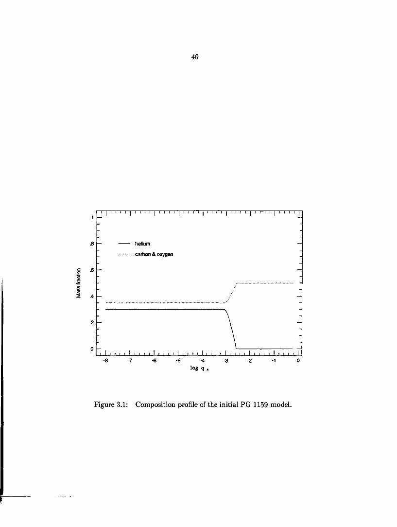
The composition profile of the initial model is given in Figure [3.1]. The compo
sition transition at log q = —3.5 was determined by the pulsation data on PG 1159
by Nather et al.(1990). The evolutionary role of this model will be discussed in more
detail in Chapter 5.
The evolution of the temperature profile as a function of effective temperature
for a 0.58 M© sequence is shown in Figure [3.2]. The temperature inversion near the
core for the hotter models is a result of neutrino cooling; this inversion gradually
disappears cis the star cools, disappearing at a temperature of 29803K, when the
model reaches a luminosity of 0.12L©. The flattening of the temperature profile near
the core at lower effective temperatures is due to the efficiency of electron conduction
in the core. This inversion is not shown in the models of TFW, for the simple reason
40
1 —
.8 (— helium
carbon & oxygen
.6 I-
.2 -
log q.
Figure 3.1: Composition profile of the initial PG 1159 model.
41
that they do not include neutrino emission; they were primarily interested in modeling
white dwarfs at cooler temperatures. They do show the isothermal core as a result
of the electron conduction. IT include neutrino losses, and show the temperature
inversion; in their helium sequence, this inversion disappears when L ~ O.lL©. Wood
does not give structural detail to make a comparison.
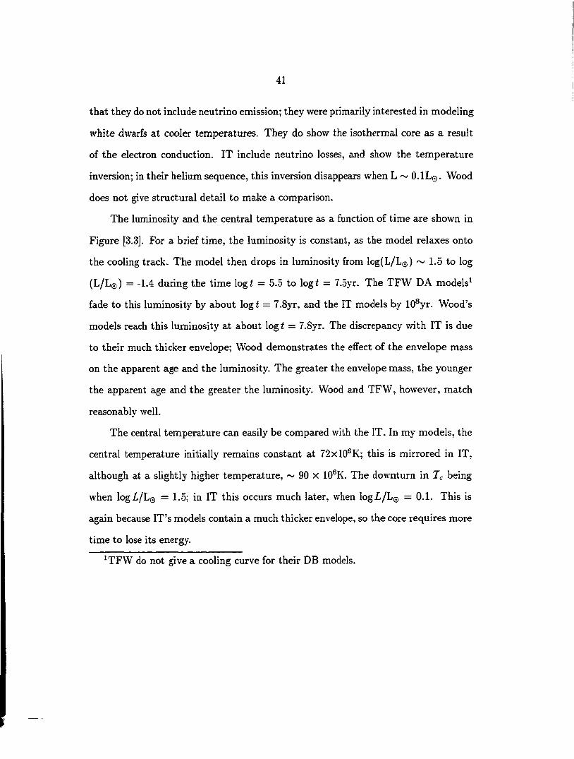
The luminosity and the central temperature as a function of time are shown in
Figure [3.3]. For a brief time, the luminosity is constant, as the model relaxes onto
the cooling track. The model then drops in luminosity from log(L/L©) ~ 1.-5 to log
(L/L©) = -1.4 during the time \ogt = 5.5 to logi = 7.5yr. The TFW DA models^
fade to this luminosity by about log t = 7.8yr, and the IT models by 10®yr. Wood's
models reach this luminosity at about log t = 7.8yr. The discrepancy with IT is due
to their much thicker envelope; Wood demonstrates the effect of the envelope mass
on the apparent age and the luminosity. The greater the envelope mass, the younger
the apparent age and the greater the luminosity. Wood and TFW, however, match
reasonably well.
The central temperature can easily be compared with the IT. In my models, the
central temperature initially remains constant at 72xlO®K; this is mirrored in IT,
although at a slightly higher temperature, ~ 90 x 10®K. The downturn in Tc being
when logZ/L© = 1.5; in IT this occurs much later, when logZ-/L© = 0.1. This is
again because IT's models contain a much thicker envelope, so the core requires more
time to lose its energy.
^TFW do not give a cooling curve for their DB models.

42
138,054K 75.049K 45,556K 27,900K 24,722K 21.229K
Figure 3.2: Temperature profile evolution

43
8
7.9
7.8
7.7
7.6
7.5
1 J L I ' L 2 3 4 5 6 7 8
log t (years)
Figure 3.3: Luminosity and central temperature evolution.

44
3.6 Summary; What ISUEVO Does
The purpose of this chapter is twofold. First, to explain the techniques and
the physics of models of stellar evolution. Second, and, most important, to establish
ISUEVO 35 working, reliable code for computing such models. The physical principles
used in these models are well understood, and the mathematical techniques have long
been explored. Not only is the numerical work well established, but a sequence of
white dwarf evolution from ISUEVO - without diffusion - gives results which are
consistent with the results of other such efforts.
The innovations to ISUEVO important to this work are described in the next
Chapter, where the techniques used to include diffusion are discussed. In discussing
this work, comparison with other researchers is impossible because such an integrated
evolution and diffusion computation, over such a span of white dwarf temperatures,
has not previously been done. Instead, we must content ourselves with an analytic
demonstration, that the results are physically plausible. Finally, after the background
work in this Chapter and the next, where I establish the reliability of the code, in
Chapter 5 I will examine the modeling of the evolution of PG 1159 with diffusion.

45
CHAPTER 4. ISUEVO II: CALCULATING DIFFUSION IN WHITE
DWARFS
Any theory too complex to fit on a T-shirt is probably wrong.
- H. Shipman (1987)
As discussed in Chapter 2, the numerical solution of the time-dependent diffusion
equation, has had very little treatment compared to that given the stellar structure
equations. As described in the previous Chapter, we have used standard methods
of solving them; the process of stellar evolution is understood well enough so that
one can, at least qualitatively, know if the solution method is providing the "right"
answer.
In this Chapter, I discuss the diffusion equation, and the methods to solve it
within an evolving stellar model. First, I will discuss what is meant by the term
"diffusion", and the various processes involved. I then discuss the historical approach,
which is essentially the work of Evry Schatzman, and contrast this with the current
approach. I then elaborate on the numerical methods used to solve this equation,
and conclude with a discussion of the physical properties of its solution.

46
4.1 Nomenclature: What is diffusion?
There are often several different connotations applied to the word diffusion.
Diffusion, in the astrophysical context, is often divided up into different categories,
depending on the driving force. In this work, "diffusion" is any process which can
cause a change of relative abundance of species within a mixture; most of the specific
mechanisms that will be discussed are a subset of this broad category. By this
definition, radiative levitation (discussed in Chapter 2) is also diffusion, although it
is not included here.
The more specific types of diffusion are gravitational settling, which is caused by
differential gravitational forces on ions. "Ordinary" or "chemical" diffusion is driven
by fractional number density gradients in a mixture, e.g., an interface between two
mixtures of differing composition. Finally, there is "thermal" diffusion, caused by
temperature gradients between two mixtures. The distinction between these various
flavors of diffusion will be made more clear as we examine the equations governing
diffusion in detail.
4.2 History: A Schatzman Sampler
One of the first quantitative approaches to diffusion in white dwarfs was given by
Schatzman in the 1950s and summarized in his classic book White Dwarfs (Schatz
man 1958; hereafter simply "Schatzman"). Schatzman considered an electric field
within a star caused by the gravitational separation of electrons and ions. This
electric field is given by Schatzman's Equation [5-81] as
E = -{iirrih - m^)ge~^ (4.1)
47
where fi is the mean molecular weight, g is the gravitational acceleration, and the
other terms have their usual meaning (see Appendix A.) The net force is then (Schatz-
man Eqn. [5-82])
Amng + ZeE = gmhZ[{AIZ) - /z], (4.2)
where A is the atomic mass, Z is the atomic charge. The net force is dependent on the
difference between the molecular weight and the mean molecular weight. Intuitively,
this is as one expects; the light elements in a mixture should float to the top.
By using an analogy of viscous forces on stellar motions in a cluster, Schatzman
then gives the following formulation for the diffusion velocity ti; of a heavy element
in the hydrogen layer of a white dwarf: (Schatzman Eqn. [5-84]):
mngZHA/Z) - APT'
T:NhmhZ^e'^[kT
where di is the average distance between hydrogen atoms. The log term is expanded
in a Taylor series, requiring that
= 10-^°"^2rZ-V'^' = A<l, (4.4) Zi c
which is effectively assuming that the thermal energy is small with respect to the
electrostatic energy.
Assuming that the outer hydrogen layer is in radiative equilibrium, Schatzman
arrives at the following expression for the diffusive velocity,
gA /'47r\^/^ w = ^ (y) {plmH)-"\R.T)-"\ (4.5)
where FL is the stellar radius.
Schatzman uses this equation to calculate some representative values for the
diffusion velocity. For the specific case of oxygen, using values of T = lO'K, Nh =

48
6 X 10^® cm~^, and g = 10® cm sec^, he arrives at a diffusion velocity of tt; ~ 2 x 10"'
cm/sec. Given a stellar size of 0.01 R©, or 10® cm, this further leads to diffusion
equilibrium times (in this context, the time it would require the element to cross
the region of interest) of about 2 x 10® yr for the outer layers, and 10® to 10® yr
for the entire star. For comparison, a young, hot white dwarf (Teff ~140,000K)
will cool to ~60,000K in 2 million years, and to ~20,000 K in 10® years. While
these diffusion timescales show that the composition could be altered over the time
of evolution, Schatzman actually concludes that diffusion alone could not modify
the surface composition, because any hydrodynamic motion would offset the small
diffusion velocities.
4.3 The Modern View of the Diffusion Equation
While essentially correct, the above view needs adaptation for use in full evolu
tionary models. In particular, the time dependent change in the diffusion velocity at
each layer within a model needs to be calculated. Thus in this "modern view'' the
physics of diffusion is set in terms adaptable to numerical computations.
The time-dependent change in number density due to diffusion is fairly simple;
for any given element with a number density n, the rate of change is given (in spherical
symmetry), by dn 1 diwr^n) ..
where w is the diffusive velocity, and n is the number density. One of the difficulties
with this equation is that it is a partial differential equation, explicitly containing the
time derivative. The structure equations, at heart, are a set of ordinary differential
equations, solved for a static sequence of models. This implies a completely different

49
approach is necessary for diffusion.
The diffusion velocities w obviously play a key role in the solution of the diffu
sion equation. While the appearance of the diffusion equation is relatively simple -
and its solution correspondingly difficult - the diffusion velocities are almost exactly
the opposite. The diffusion velocities are given by Burgers (1969), Equation [18.1],
where I have simplified by ignoring thermal effects and magnetic fields. The diffusive
velocity Wj of a species j is then determined by
^ o-Kijiv/i - vfj) = Vpj - —Vp - ZjUjcE (4.7)
» P
where the sum is taken over the M elements in the mixture and electrons. A',j are the
resistance coefficients, E is the electric field, and all other symbols have their usual
meaning. For a mixture of M elements, equation [4.7] gives a set of M independent
equations for M + 2 unknowns. There are M-f-1 densities, {M elements -f electrons),
but since A',j = A'j,-, the equations are not all independent; the electric field E is
treated as another unknown.
The resistance coefficients A',j, inversely related to the diffusion coefficients used
by some authors (see Eqn. [4.37]), can be viewed as representing a viscous force
resisting the diffusive movement. They are derived from consideration of inter-atomic
collisions and scattering. The resistance coefficients used here were obtained from the
calculations of Paquette et al.(1986a, PPFM), who used a static screened Coulomb
potential to calculate the impact integrals. They published their results as analytic
fitting functions for the coefficients. Our resistance coefficients are computed from
their fitting tables, eliminating the need for extensive calculations or less precise
approximations.
Though it might be possible to arrive at an analytic solution for the diffusion

50
velocities to compare with Schatzman, this would not be very illustrative. The very-
nature of this work is an examination of the dynamical nature of diffusion. The
diffusion velocities, as will be seen, vary widely within a star. To calculate a sin
gle velocity, or extrapolate a timescale from this velocity, would be an inadequate
comparison. Instead, velocities calculated from Eqn. [4.5] will be compared to the
numerical solutions in the next section.
4.4 Solving the Diffusion Equation
4.4.1 Numerical methods
With the paucity of treatments of dynamical diffusion, there are no "standard
methods" for the diffusion equation in white dwarfs. The works which have the most
sophisticated treatment for diffusion, Pelletier et al.(1986), Muchmore (1984), and
Iben & MacDonald (1985), all follow different approaches. Further, in addition to
simply solving the diffusion equation, there was an additional constraint that was
placed on the method to be used here: it had to be incorporated within a working
stellar evolution code, ISUEVO. This strongly encouraged the selection of a finite
difference method, rather than a finite element method such as used by Pelletier et
al.(1986).
The first simplification made is the assumption of spherical symmetry. The effect
of this is to replace V/ with Non-spherical effects in diffusion are most likely
of lower order of importance than non-sphericity in dynamical processes, although
the study of Vauclair and Reisse (1977) indicates that circulation from rotation may
be important. However, since the equilibrium, model is constrained under spherical
symmetry, consistency requires that diffusion be treated as spherically symmetric.

51
The equation for the diffusive velocities, Equation [4.7] is not a linearly inde
pendent system, since we have M equations and M + 2 unknowns. So we follow the
method used in Muchmore (1984) and IM, and introduce the steady-state constraints
of no net mass flow and no net current, that is,
M+l
^AiWi = 0 (4.S) i
Af+1
Ziewi = 0 (4.9) i
Despite its apparent complexity, the set of equations [4.7, 4.8-4.9] gives a simple linear
system of equation for the diffusive velocities for all elements present. In practice,
subroutines from the Numerical Analysis Group (NAG) are used to solve this linear
system, although nearly any linear equation solver library would suffice.
In order to solve the diffusion equation, we invoke a simple technique known as
the method of lines. First, the spatial derivative in Equation [4.6] is discretized with
centered differences, as follows: ^
(4.10) drij _ 1 Tij+iWj+irj^i -
dt ~ r] 2(rj+i-rj_i)
We then, as in IM, invoke the boundary conditions that
n —> 0 as r —>
and
dn . . -^r > 0 as r —> 0 or
For N layers in the model, this gives riN+i = 0 and no = ni, where layers
N + l and 0 are "pseudo-layers" considered for the application of adding boundary
^In the following section, the subscripts j represent the quantity at layer j within the model, contrary to the earlier notation, where subscripts referred to element j.

conditions. We then have following set of equations:
dn-i _ 1 7121^2^2 dt r? 2r2
(4.11)
dt r? 2(r^+i-r ,_x) "" ^
driN _ 1 njv-iU7;v-ir^_i dt r%2{risf+i-r^-i)
For each element in the model, this gives a system of N ordinary differential
equations to be integrated for some timestep St. For a typical model, there are about
300 zones.
To integrate equations [4.11-4.13], the entire system is integrated by a numerical
library subroutine DEBDF. This is a backward differentiation formula initial value
problem integrator, part of the DEPAC library by Shampine and Watts (1979). This
integrator was selected because of its ability to handle stiff differential systems, as
well as its simplicity to implement in the evolution code. The integration must be
carried out separately for each element in the model.
This method was chosen for several rezisons. First, the spatial discretization
could be simply carried out using the existing model grid, which allows the diffusion
computation to be incorporated much more easily into the evolution code. Second,
it allowed for treatment of as many elements in a mixture as desired. And third, it
allows the use of an existing software library, with known numerical behavior, for the
integration of the ordinary differential equations.
The differential equations are assumed stiff for the solution scheme. This is
partially justified by the observation of Pelletier et al.(1986) that diffusion timescales
can vary widely throughout the star. Even if incorrect, this assumption only affects
the numerical method used; a stiff problem solver is typically less efficient on non-stiff

53
problems. In order to integrate a stiff differential equation, we need to calculate the
Jacobian J,j = dfi/drij^ of the above system, where /,- are the right-hand sides of
equations [4.11-4.13]. Because of the centered differences used in the system, it is a
simple banded matrix containing only the ±1 off-diagonal bands, given by
T - lW2 •^1.2 -
1
rf 2(r,+i - r,_i 4.-1 = -To.- "J. 2<i<iV-l (4.15)
•'i.i+i = -1 -ISiSJV-l (4.16) rf 2(r,+i - r,_i)
T 1 wn-IRN-I
J- j = 0 otherwise. (4.18)
This also gives another reason for selecting the DEPAC library. It is possible to
specify a banded Jacobian matrix structure to the DEBDF routine, thus allowing
more efficient computation.
4.4.2 Timestep control emd the quasi-static assumption
Since this system must be integrated separately for each element, a "queisi-static"
assumption is made. For some timestep 6t, the equations are integrated for each
element, assuming that changes in the composition profile for one element will not
affect the diffusion of another element over the timestep 6t. Only after all elements
in the mixture have been integrated are the composition profiles updated for the next
St. This assumption constrains the choice of 8t.
The cooling timescales of the star are on the order of 10^ to 10' years, depend
ing on the effective temperature. For the thin, outer layers, this is nearly always

54
much longer than the diffusion timescales, so given an evolutionary timestep At, we
integrate the diffusion equations for a series of shorter timesteps St, until we reach
At. A larger timestep allows the diffusion to be calculated with fewer integrations,
thus minimizing computation time. However, a larger timestep also allows for greater
change in the composition profiles, thus violating our quasi-static assumption. We
therefore begin with an arbitrary 5 year 6t timestep. Each element is diffused for 8t,
and then the meiximuin relative change in composition at any point for all elements
is determined
/'"'•.new-n-,old\ Anmax = max , (4.19)
' \ «;,new /
where
n. QJ JJ = initial number density at layer i (4.20)
Wj,new = final number density at layer i (4.21)
Given such a maximum Anmax, the new timestep is then given by
Thus a composition change greater than 15% at any point in the model will cause
a decrease in the timestep used. This method allows for the timestep to adaptively
increase as the compositional structure approaches diffusive equilibrium, and yet
maintains the quasi-static nature of the calculation. The values of 5 years and 15%
were arbitrarily selected, as a compromise between retaining the quasi-static nature
and speed of calculation.
There is also a third timestep here, one used internally within the DEPAC li
brary. When the DEPAC library is called, it is instructed to integrate the diffusion

55
equation over the timestep St. The DEPAC integrator uses whatever timestep needed
to accomplish this integration and maintain a specified error tolerance. The error tol
erances were set at lO""* for the relative error, and 5 x 10~® for the absolute error.
This allowed rapid computation, and is consistent with the error tolerances used in
the other parts of the code.
4.5 Diffusion Velocities — Representative Results
Representative diffusion velocities for helium in a PG 1159 model are shown in
Figure [4.1]. Also shown in this Figure is the helium composition profile. As can
be seen, the diffusion velocity is a smooth curve near the outer layers of the star.
The shape of this curve will be explored more in the next section; note for now that
the diffusive velocity is higher near the surface, and thus the outer regions will reach
diffusive equilibrium before the inner regions. Further, there is the negative spike in
the diffusion velocity at the interface between the helium envelope and carbon/oxygen
core, at a mass fraction of about qs = 10"^. The negative diffusion velocity is a result
of the helium being forced inward by the steep number density gradient at the core
boundary.
We can compare the diffusion velocities with those calculated using Eqn. [4.5].
Given a stellar radius for this model of 1.67 xlO^cm, we can re-write Eqn. [4.5] as
= 1.201 X cm/s (4.23)
This allows us to compare the diffusion velocity calculated with Schatzman's method
and Burger's formalism directly. A comparison is given for the oxygen diffusion
velocity at two locations in the star in Table [4.1]. With its higher Z, oxygen will be

He Diffusion velocity
He Mass fraction
Figure 4.1: Diffusion velocity for PG 1159 model

57
most likely to conform to the constraint in Eqn. [4.4]. Nearer the center of the star, at
log 9 = —3.1, the diffusion velocities from the two different methods are comparable.
As can be seen, however, near the surface, there is a large discrepancy in the two
different methods, of nearly an order of magnitude. This is explained by the last
column, the condition expressed in Eqn. [4.4]. The limit under which Schatzman's
equation is valid (A < 1), is violated in both locations. However, this departure is
exaggerated near the surface, as A increases due to the greatly decreased density.
Thus Schatzman's expression in Eqn. [4.5] is inapplicable without further correction
over most of the range of physical parameters in this model.
Table 4.1; Oxygen Diffusion Velocity Comparison
log q logflr log/!) log T (cm/s®) (gm/cm^) (K)
ix7(Schatzman) t<;(model) A (cm/sec) (cm/sec)
-3.1 -7.0
7.675 3.002 7.753 7.486 -0.288 6.948
1.206 xlO"® 4.416 xlO"® 9.7 2.464 xlO"® 1.889 xlO"" 37.1
4.6 Physical Explanation of the Diffusion Velocities
As mentioned in the previous chapter, comparison of these results with other
authors is impossible since no other work exists. Instead, we must satisfy ourselves
that the results are reasonable by using a more analytic approach, and examine the
physical forces which drive the diffusion. The diffusion equations are complex, and
understanding the solution in an intuitive way can be difficult. Still, with a little
mathematics, the physical basis for these results can be made clearer.
In determining the diffusion velocities, there are two competing processes, the

58
driving - the differential forces acting on the ions - and the resistance - the viscosity
caused by atomic collision. The driving is determined by the physical conditions,
mostly temperature, pressure, and number density gradients. The resistance is more
a function of inter-atomic interactions and dynamics, but is also dependent on the
conditions. The interplay of these two processes determines the resulting diffusion
velocity behavior. First, we examine the forces responsible for species separation,
then we will examine the resistance to diffusive movement.
4.6.1 The driving forces
To begin with, the right hand side of Equation [4.7] is what I will refer to as the
"driving force" of the diffusion, denoted by — V'j- That is, we have
= Vp," - - Zjnj-eE, (4.24) P
= ViuikT) - - ZjnjeE, (4.25) P
= kTVrtj + rijVkT - ̂Vp - ZjujeE. (4.26) P
At this point, we can identify the term containing Vnj as "chemical diffusion",
reflecting number density gradients. One might be further tempted to identify the
VfcT term as thermal diffusion, but this is incorrect. Thermal diffusion is the inter
connection of diffusion and heat flow, which has been neglected here. This term can
be better understood by continuing its breakdown, as follows;
= kTVn, + n;V--^Vp-ZjnjeE (4.27) n p
= kTWrij -t- - ̂ Vn - ̂ Vp - ZjU^eE. (4.28) n p
Noting that pj = mjrij and p = fimhn, we have
= kTVnj - njkTV In n + _ ZjnjeE. (4.29)
59
Hydrostatic equilibrium allows us to replace Vp with —pg. Defining the number
density fraction Xj = Wj/n, we have
-il>j = kTXjVn + kTnVXj - kTXjVn —{fimh-Tnj)njg — ZjnjeE.{^.ZO)
The Vn terms cancel, giving the following:
1 2 3
—il^j = nkTVXj — — rnj)njg — ZjujelE. (4.31)
The three terms can be identified with three different driving mechanisms as
follows. The first term depends on the fractional number density gradient. This is
typically called "ordinary diffusion" or "chemical diffusion". This term depends on
the gradient of the fraction number density and not on the total number density. The
second term is proportional to the gravitational force; and depends on the difference
between the particle mass and the mean mass of the surrounding material. This
"gravitational settling" term guarantees that lighter and heavier elements separate.
This term is directly proportional to the gravity; this is also in accordance with
our intuition, since the pure surface layers observed in white dwarfs indicates that
diffusion operates more efficiently in these objects compared to the main sequence.
Finally, there is the electric field term, which arises from the fact that diffusion is
acting on charged particles. Although not apparent here, this term is related to the
gravity eis well, since the source of the electric field is a separation of electrons and
ions caused by the gravitational field. In practice, the electric field is treated as an
additional unknown to be calculated.
The forces driving the diffusion are plotted in Figure [4.2] for the PG 1159
model shown in Figure [4.1]. Clearly, the major force in driving the diffusion is the
gravitational force, except for the interface near the core boundary. Near the core.

60
there is a large contribution from the chemical term, caused by the steep decrease in
the helium in the core.
Shown in Figure [4.3] are the driving terms near the surface, where the vertical
scale has been expanded roughly by a factor of 100 over the scale in Figure [4.2]. Since
the surface of this model heis a homogeneous composition, and thus no composition
gradients, there is no contribution from the chemical diffusion term. The electrical
and gravitational terms dominate.
Examining Figures [4.1]-[4.3] , it is apparent that the greatest diffusion velocity
is at the surface, while the greatest driving takes place near the center of the star.
In order to resolve this apparent contradiction, we must now take a look at the left
hand side of Eqn. [4.7] and examine the behavior of the resistance coefficients.
4.6.2 The resistance coefBcients
To fully understand the diffusive motions, we must understand the nature of
the resistance coefBcients. However, as I will be following the description given in
PPFM, who in turn base their work on the formahsmof Chapman & Cowling (1970),
I will start by deriving the diffusion coefficients, which have a simple relation to the
resistance coefficients used here. This is not an analytical analysis of the resistance
coefficients; rather, I will derive simplified approximations to illustrate the functional
dependence of the resistance coefficients on the stellar parameters.
According to PPFM (their Eqn. [5]), the first approximation^ to the diffusion
^Di is the first approximation. While I will not use higher approximations, i.e. D2,I will keep the subscript to keep notation consistent with PPFM.

61
S 0 Q> 1 s
QO C 5 u a a X
2xl0" ^ 1 1 1 1 1 1 1 1 i 1 |"i r 1 1 1 1 i 1 i 1 1 1 1 i 1 1 [ 1 1 t i 1 1 T 1 r [-
' ~ J
10" _ 1 /
1
I
0 _
/
/
I -
0 -
(
_ i
-10" — chemical \ —
-2xl0" —
gravitational \ V\
electric \ \"
sum \ \ —
-3xl0" — \ —
-4xl0" " 1 1 1 1 t 1 ) 1 1 1 1 » » > » 1 1 1 » ) 1 1 1 » 1 1 ! 1 1 1 1 t 1 1 1 1 1 1 1 1 u
-8 -7 -4 log q.
-3
Figure 4.2: Diffusion driving for PG 1159 model

0
,s 10' chemical
gravitational electric sum
-2x10'
-3xl0'
-4x10® -5.5 •5 -6.5 •6 -7.5 •7 -8
log q.
Figure 4.3: Surface diffusion driving for PG 1159 model

63
coefHcient of two elements is given by
where
op [A,]. = (4.32)
n = ns + Tit, (4.33)
m = TUs + TUt , (4-34)
^
Mi = Ai = s,t) (4.36) rus + mt
where the subscripts 5 and t refer to each species, and is the "collision integral,"
and the superscripts i and j represent moments of the integrals. Since the resistance
coefficients are related to the first approximations, we will not be using higher mo
ments of the collision integrals. The resistance coefficients are related to the diffusion
coefficients by
kT K,t = X,Xtnj^ (4.37)
[^sth
where Xi is the fractional number density of species i.
The collision integral is in turn given by PPFM Eqns. [18-21] as
where
0^4' = 2 t f {1 - cos ' x s t )bdb (4.39) Jo
and
Xs t = -2 bdr i r Jr?'' r2 g^kT
(4.40)
64
V^i(r) is the interaction potential, and is the distance of closest approach of the
two atoms, given by
, Vsiirt") g ( r f f ' y g H T
Despite the apparent complexity, these terms have rather simple physical inter
pretations, in that they describe a classical collision between two particles interacting
with potential Vstir). are related to collisional cross sections^ after integrating
over Maxwellian velocity distributions. The integrand g in Eqn. [4..38] is a dimension-
less velocity. are collisional cross sections for a given energy, integrated over the
impact parameter b. Xst is the scattering angle, integrated over the distance between
the particles. Further approximations will simplify these integrals, keeping in mind
that our final goal is an understandable expression for the resistance coefficients as a
function of the stellar parameters.
The details of what follows can be found in PPFM. First we assume a pure
Coulomb potential, of the form = ZsZte^/r; the integrals are then
where
A. = (4.42)
and
Xd =
^The superscripts represent moments of the integral. While most higher order moments are unused, the superscripts are retained to maintain consistency with the notation in PPFM.

65
Xd is the Debye length, the effective range of the Coulomb potential in an ionized
plasma, where the Coulomb interaction is "screened" by intervening ions. Such a
"screened" potential follows the form of
G-r/Az, K(r) = Z,Zr
r2
We now make a second approximation, and ignore the velocity dependence of the
term in Equation [4.41], replacing it with an average value of the dimensionless
velocity, < >= 2. This gives (PPFM Eqns. [29], [31], & [33])
- - i W f ' 41' = ln(l+7'j, (4.45)
and
_ ikTXp
~ ZsZte^' ^ ^
Finally, we integrate over the velocity distribution to obtain the collision integral,
which, with the given assumptions, becomes (see PPFM Eqn. [34])
\2TrmM,Mt) V ^ '
We are nearly there. Remember that the initial goal of this exercise was to
arrive at a simplified analytic expression for the resistance coefficients, in order to
understand the diffusive behavior. The resistance coefficient, from Eqns. [4.32],
[4.35], and [4.37] is given by
2kTnm
ZE ' (11)
^ ^ ^2kTm8MsMtnYt = X.X,n — — ,
= (4.48)
66
Now, using the the definition of fij/' from Equation [4.47], and some algebra, we
have
K., = %X.X,n-( 3 \ 2x771 (ArT)
Approximating m,- ~ Airtih-, we have
yN2.Z,eYla(l + |0) (4.49)
jr _ 47r XsXtn2 ( AgAt \ ^ 7272 4 V25r(A:r)3m/,(^ + ^,)j
A-., = 3.275.10'XxyzfZf(p;^^^^)'x
I n ( 1 + 2 . 3 9 5 ( 4 . 5 1 )
I will make another approximation, and neglect the logarithmic term, since the
dependence will dominate. This leaves us with
Kst = 3.275 X 10^° XsXt^ gm • cm'^ • sec-\ (4.52)
We have now reached the goal of a simple analytic form approximation to the
resistance coefficients. Eqn. [4.52] relates the resistance coefficient to the model
parameters of density and temperature. While not precise enough for actual modeling
- indeed, the entire point of PPFM was to avoid the various approximations used
here - it does give us an idea of the behavior of the resistance to diffusion within the
stellar interior.
The net result can now be stated quite simply. The diffusion driving force, given
by Equation [4.31], depends on the number density. The more atoms of a given species
present, the greater the total force. If we neglect the temperature dependence, the

67
resistance to diffusion given by Equation [4.52] depends on the square of the number
density. This is because the resistance depends on the inter-atomic interaction, which
goes roughly as the square of the number of ions present. Thus, the highest velocity
is found in the lowest density regions, i.e., near the surface.
Now that we have a physical description of the resistance coefficients, let us
examine their behavior in the models. The sum of the resistance coefficients, as given
by the tables in PPFM, is plotted in Figure [4.4]. The resistance coefficients vary over
10 orders of magnitude between the surface of the model and the core. Where the
driving forces increase by roughly a factor of 100 from the surface to qs = 10~®, the
resistance coefficients increase by over a factor of 1000. So even though the driving
force is weakest at the surface, the resistance to diffusive motion increases faster than
the force as a function of depth, and the net effect is the highest diffusion velocity is
at the surface.
4.7 Summary: What Just Happened
In this chapter 1 presented a detailed description of the diffusion equation, and a
description of its numerical solution. We have also examined the behavior of the dif
fusion velocities within our models, and looked at the important physical parameters
which govern its behavior. The most important idea is that equilibrium is reached
from the outside in, and the governing factor is the resistance to diffusion determined
by the resistance coefficients.
As I have shown, diffusion has its greatest impact in the outer layers of the
model, where the resistance is lowest. It is in these very layers that we can also
probe the structure of stars, using the tools of stellar pulsation theory. In the next

68
Figure 4.4: Resistance coefficients for a PG 1159 model
69
chapter we will examine the changes in compositional structure due to the diffusion
in an evolving model, and, most importantly, compare the resulting models with
observation.

70
CHAPTER 5. EVOLUTION RESULTS - TRANSFORMATION OF
THE HELIUM STARS
The light which reveals to us the existence of the heavenly bodies also
bears the secret of their constitution ...
James E. Heeler (1897)
In this Chapter, I describe the results of a calculation of a sequence of helium-
rich white dwarf models. This sequence represents the evolution of a PG 1159 star as
it cools and becomes a "normal" DB white dwarf. PG 1159 stars are an important
starting point because they lie at the top of the white dwarf cooling track. Many of
the PG 1159 class - including the prototype PG 1159-035 - are also pulsating stars;
these pulsations allow a probe of the interior structure of the star, thus a better
understanding of the changes that take place during the evolution of a white dwarf.
This Chapter discusses the evolution of the sequence that includes diffusion beginning
at the PG 1159 stage. Using this starting model, I show that a direct evolutionary
link can exist between the PG 1159 stars and the much cooler DB white dwarfs below
the DB gap. The model that results from evolution from the PG 1159 temperature
regime to below the DB gap is then subject to the same sort of stringent test passed
by the initial model: comparison of its oscillation frequencies with those observed in
the pulsating DB white dwarf GD 358.

71
5.1 The Initied Model
The initial model weis designed to model the observed pulsational spectrum of
PG 1159, and is based on the evolved core of a post-AGB star. The model was ini
tially evolved to the AGB and the formation of a carbon/oxygen degenerate central
core by Iben (1984). This model was removed from the AGB during a thermal pulse,
and so is representative of the probable progenitors of DB white dwarfs. Kawaler
Sz Bradley (1994) modified the outer layers of the model in a systematic way, evolv
ing the starting models into the PG 1159 regime for comparisons with the WET
observations of this star reported by Winget et al.( 1991a). For this investigation,
the important point of the initial model is that it is an accurate model of the star
PG 1159 that matches the observational constraints both from the spectroscopy of
Werner et al.(1991) and from its observed oscillations.
The composition profile of the initial model is shown in Figure [3.1]. The en
velope, down to a depth of logg = 10"^'^ is set to a uniform composition of ^He
30%, 35%, and 35% by mass. These abundances are consistent (within the
uncertainties) with the atmospheric models of Werner, Heber, k Hunger (1991a),
who find (by mass) helium at 0.33, C at 0.5, and 0 at 0.17. The most important
feature of the composition profile is the composition transition at log q = —3.5. This
is a direct result of the investigation by Kawaler & Bradley (1994); the location of
this transition is determined from the pulsational properties of PG 1159.
By the time the model approaches the PG 1159 regime, nuclear burning has
ceased. This allows initial models of stars of different maisses to be obtained from
the original model by re-integrating the equations of structure, after changing only
the mass of the model. In this process, the dependence of fractional luminosity and

72
composition as functions of the fractional mass are preserved. Some iteration on
the surface luminosity is necessary in these integrations to ensure satisfaction of the
surface boundary conditions. With this procedure, as long as the mass did not differ
too much from the original 0.59M© model, the resulting models should be accurate
representations of stars that have similar evolutionary history through the thermally
pulsing AGB.
5.2 The Diffusion Sequence
The results of the evolution and diffusion calculations are described in Dehner
& Kawaler (1995). Some of the results presented in that publication are also given
here, along with additional data and discussion not presented in Dehner & Kawaler
(1995) due to space constraints.
To examine a range of predecessor masses, we computed four evolutionary se
quences, ranging from O.56M0 to 0.62M©. The results of the calculations show lighter
elements float to the top, while heavier elements sink to the core. This is summa
rized in Figure [5.1], which shows the ''He mass fraction for models of several effective
temperatures in the O.SSM© evolutionary sequence. As the model cools, the helium
abundance increases in the upper layers; when the model reaches 80,000K the mass
fraction of helium at the surface has reach reached nearly unity, and the mass fraction
of the He transition zone has reached a depth of log q = —5.0.
The corresponding helium diffusion velocities for this model sequence are shown
in Figure [5.2]. As the model evolves, the diffusion velocity drops near the surface.
This reflects the increase of the helium composition in these layers, and the decrease of
the mean molecular weight. As seen from Eqn. [4.31], as the mean molecular weight

73
I I I I I I I I I I I I I I I I I I I I I I I I I I I I I I I I I I I I I I I I
= 138,054K • \ \ \ \ = 75.987K
N \ \ = 46.109K \ \ \ T« = 28,613K \ \ \ = 24,121K \ \ \ = 20.850K
- \ \ \ \ \
^ \ \ ^ \ x
^ \ \ ^ \ \
—^
0 — I I I I I I I I I I I I I I I I -7
I I I , . I
-5 -4 Log q.
t 1 1 I I » I t I I > I I > I I I I 1
Figure 5.1: Helium composition evolution

74
// approaches the atomic weight of helium, the driving force for the diffusion (on
helium) will decrease. As the helium fractional abundance increases towards unity,
the abundance of other elements will decrease; this decrease will cause a decrease in
their driving, due to the number density dependence of the gravitational term. This
change in // can is seen in Figure [5.3], which shows the mean molecular weight n as
a function of mass fraction for the models in Figure [5.2].
The evolution of some of the more important parameters in the 0.58 M0 sequence
are given in Table [5.1]. The location of the helium to carbon transition zone is
difficult to define in models where the helium has not yet formed a clear surface
layer, until about 41,OOOK in effective temperature. The log of the surface carbon
abundance (by mass) is also given. As can be seen, even at 21,000K, there is still
some carbon in the surface layers of the model.
Table 5.1: Evolution of Key Values
Teff (K) log L/(L®) Time (Myr.) log He/C trans. log surf. C 138,054 2.26 0.000 n/a -0.46 112,154 1.76 0.045 n/a -0.50 94,618 1.36 0.144 n/a -0.55 75,987 0.90 0.409 n/a -0.70 60,950 0.45 0.892 n/a -0.92 46,109 -0.09 2.022 n/a -1.44 41,159 -0.30 2.771 -7.18 -1.71 30,690 -0.85 6.857 -6.60 -2.73 28,562 -0.98 8.984 -6.44 -3.05 25,809 -1.17 14.190 -6.14 -3.61 23,377 -1.35 23,048 -5.82 -4.25 20,850 -1.56 40,781 -5.44 -4.99

75
I I I I I I I I I I I I I I I I I I I I I I I I I I I I I I I I I I I I I I I I I
Trfr = 138.054K Trfr = 75.987K Trfr = 46.109K Trfr = 28.613K Trfr = 24.121K Ttf = 20.850K
sr-
I I I 1 I r I I I I I I I I I I I r I r I I I I I I I I I I I I I I I I I I I I r I 1 . . . I -8 -7 -5 -4
log q. -2
Figure 5.2: Helium diffusion velocity evolution.

76
T«ff
1 1 1 1 1 1 1 1 1 1 1 1 1 1 1 1 1 1 1 1 1 1 = 138.054K
1 1 1 1 i - i 1 • 1 • 1 r
- T^ = = 75.049K _
T«jr = 45,556K • = 27.900K = 24,722K f
- / -
— ^ ̂ ^ / ^ y
/ / / / / /
/ /' / / / f ' / * / / /
/ / /' ./ /
—
X / /
/ / /
/
/ / _ / '
^ ̂ ^ / ^ y
/ / / / / /
/ /' / / / f ' / * / / /
/ / /' ./ /
-
1 1 1 1 1 1 1 1 1 1 1 1 1 1 1 1 1 1 1 1 1 1 1 1 1 1 1 r 1 1 1 1 1 1 1 1 1 1 1 -8 -7 -6 -5 -4 -3 -2 -1
log q.
Figure 5.3: Mean molecular weight evolution.

77
5.3 Comparing with Observation: Pulsations
An important facet of any investigation is comparison with observables. So far,
I have taken an initial model - as best determined by observation - and simulated its
evolution into a cooler star. The major result so far has been accumulation of helium
at the top of the model, with heavier elements sinking deeper. more in-depth
examination is afforded by computation of the nonradial oscillation frequencies of
the models that are within the DB instability strip, and comparison of these periods
with observations. The nonradial p—mode periods for models in the appropriate
temperature range are computed using the adiabatic pulsation codes described in
Kawaler & Bradley (1994).
As the models approach the hot edge of the DB instability strip, which is at
about 28,000K, the transition zone heis reached a depth of about log q — —6.0. The
depth of this composition transition zone, however, has observational significance, .'^s
discussed by, e.g., Kawaler (1990) and Kawaler & Bradley (1994), such a composition
transition zone produces a strong density gradient, which in turn acts as a reflecting
boundary for some nonradial modes. One signature of nonradial modes, such as
seen in white dwarfs, is that they are equally spaced in period. Those modes which
are influenced by the transition zone are "trapped modes"; they show periods that
are systematically different than untrapped modes. The signature of trapped modes
is that they are closer to the next larger period than normal modes. Thus trapped
modes appear as local minima in a plot of periods spacing as a function of period when
the the period spacing is computed in a reverse-difference form. The period spacing
itself is a function of the mass of the star, and the period difference between trapped
modes is determined by the depth of the composition transition zone (see Kawaler &

78
Bradley 1994, and Bradley & Winget 1994, and their references, for details.)
Photometric observations of GD 358, the prototype DBV, were made by Winget
et. al. (1994). These observations were used by Bradley & Winget (1994) in order
to model the structure of GD 358. While comparing models to models may be a
somewhat dubious pursuit, in this case it is useful since the models were generated
by completely different procedures. The models of BW consist of evolved white dwarf
cores with static envelopes added which were adjusted to fit the pulsational data. This
is similar to the approach of Kawaler & Bradley (1994) for the model of PG 1159
used as the initial model here. My GD 358 model, however, is not constructed to fit
any specific observations; it is simply the result of the evolutionary calculations.
When comparing the models to the observations, it is useful to compare both
the periods and the period spacing. In order to facilitate this comparison for a large
number of models, I computed the sum of the squares of the differences between the
period, and the same for the period spacing, for all models in the instability range.
That is, I computed the sums
where the sum is taken over all observed periods. The inverse of these quantities are
plotted in Figure [5.4] for all models, where the best match will be shown by peaks in
the diagram. The best model, although somewhat a matter of debate, is the 0.58M©
model with Teff=24,210K. With this model, the periods and the period spacing both
fit well to GD 358.
Now, we compare the pulsational spectra of our models with that observed by
N (5.1)

79
p-p. .4
dP-dP, .3
J2
.1
0
P-P, .4
.3
,1
0
P-P. .4
0.60 Mo .3
.2
.1
0
P-P, .4
0.62 Mo .3
.2
.1
29000 30000 27000 28000 22000 23000 24000 25000 26000 T.«(K)
Figure 5.4: Model grid to observation comparison.

80
Table 5.2; Period comparison
k Evolved BW GD 358 5 298.641 301.803 6 340.390 339.975 7 382.116 .377.734 8 423.444 420.505 423.27 9 461.782 462.336 464.23
10 494.362 499.181 (501.59) 11 534.622 535.575 (541.75) 12 577.982 575.938 (576.76) 13 619.120 616.119 618.28 14 659.920 658.426 658.35 15 699.238 701.370 700.64 16 734.684 733.988 7.34.30 17 775.708 770.358 770.57 18 817..524 812.507
the WET data and as modeled by BW. All three spectra are shown in Figure [5.5].
The hollow triangles represent data points where the identification of pulsational
modes was uncertain. A listing of the periods in our best model, BW's model, kindly
provided by Paul Bradley, and the observed periods in GD 358, from Winget et
al.(1994), is given in Table [5.2].
The pulsational behavior of the evolved model and the BW model is similar.
While there is some discrepancy at the shorter periods around 450 s, the longer
periods show the same behavior. Further, the global characteristics of luminosity
and temperature are close; as shown in Table [5.3], the evolved model falls well
within the range of values calculated for GD 358 using the model grid of BW. So
while the BW model is a superior fit to the data, the evolved model is similar to the
model of BW in many respects.

81
6
GD 358 (WET) • BW 0.61M^. 24210K
Diffusion 0.58M^ 24121K 4
2
0
•2
-4
•6
500 600 800 450 550 650 700 750 P (sec)
Figure 5.5: Period spacing comparison.

82
Table 5.3: Comparison of model characteristics
Diffusion BW best BW range TeffClO^K) 24321 24.210 24±I M (M®) 0.58 0.61 0.61±0.03 log(L/L®) -1.294 -1.308 -1.30l8-?f log(MH^/M.) -6.0 -5.82 -5.70lg:^
The carbon in PG 1159 behaves essentially opposite of the helium; it slowly sinks
to the core of the star. However, even in the coolest model the surface carbon never
reaches zero; there always remains some trace abundance at the surface. Recent
observations of GD 358 by Provencal et al.(1995) (private communication) indicate
trace carbon abundances, as observed by HST ultraviolet observations. Atmospheric
models by P. Thejll indicate that the carbon is present with a ratio of log n(C)/n(He)
= -5.5 (Provencal, 1995), while in our models the residual carbon abundance gives a
log ratio of -4.5. Further, they predict a somewhat higher surface temperature then I
do, at Teff ~ 28,OOOK. While there is a modest discrepancy here, it is apparent that
the carbon abundance can be explained by a dilFusive tail, without invoking more
exotic scenarios such as radiative levitation or accretion.
5.4 Conclusions: the PG 1159 — DB link
This model sequence demonstrates how a PG 1159 star may evolve into a DBV
star like GD 358. The key factor in this conclusion is the pulsational data of GD 358,
and the comparison with the model properties. Not only does the pulsational spec
trum fit the observations, but the model is also consistent with the independently
derived model of BW. This is significant because BW is specifically constructed to fit

83
the observational data, while my model is simply evolved from the PG 1159 stage.
This then shows one definite path in white dwarf spectral evolution, between
PG 1159 and GD 358. It shows at least one possible predecessor of GD 358, and
a fate of PG 1159 stars. Further, with the identification of these stars as the same
star at different evolutionary states, this simplifies considerations of previous stages
of stellar evolution. Post-AGB evolutionary models now have to account for one less
type of white dwarf, if the PG 1159 and DBV stars are the same.
A key weakness in this investigation is the lack of hydrogen in the models. Be
cause of this, the models maintain their helium rich appearance at all evolutionary
stages. This is in direct conflict with the existence of the DB gap. The simple exis
tence of this gap indicates that all white dwarfs must contain (or acquire) hydrogen
during their cooling lifetime, before reaching Teff ~45,OOOK. While the spectroscopic
analysis of PG 1159 by Werner et al.(1991a) indicates very little hydrogen, the con
sequences of hydrogen in the evolution of a PG 1159 model are explored in the next
Chapter.

84
CHAPTER 6. THE HYDROGEN MODELS
Second verse, same as the first - a little bit louder and a little bit worse
Traditional
In this chapter, I describe calculations of the evolution of a PG 1159 model with
a small amount of hydrogen added. As discussed in previous Chapters, observations
constrain the hydrogen content of the surface of PG 1159 to be very small, less than
5% by mass. The previous Chapter demonstrated that PG 1159 stars can be the
ancestors of the DB stars except for the fact that such a link requires that the DB
gap be ignored. Adding a small amount of hydrogen to the PG 1159 models could in
principle lead to their becoming DA stars at the appropriate temperature range; this
raises the interesting possibility that PG 1159 stars could represent the progenitors
of all white dwarfs, as has been suggested in the so-called "single-channel" models
of white dwarf chemical evolution (see, for example, Shipman 1989, and Liebert et
al.l987). In order to investigate the effects of hydrogen on the evolution, a small
amount was added to the surface of the initial model.
6.1 The Initial Model
The initial model for investigating hydrogen was based on the PG 1159 model
discussed previously. There were three major constraints that were considered when

85
adding the hydrogen to the model. First, the total hydrogen mass wcis to be less
than 1O~^°M0. This limit is determined from Liebert et al.(1987), who argue only a
very thin hydrogen surface layer can be convectively overturned at the red edge of
the DB gap. Second, the surface abundance of the hydrogen was to be (at most) 5%
by mass, to be consistent with the spectroscopic observations as modeled by Werner
et al.( 1991a). Finally, the hydrogen was not to extend deep enough into the stellar
envelope to ignite; it was assumed that the models had evolved to the stage where
nuclear burning would cease. While this last assumption may be somewhat arbitrary,
it allowed a reasonable starting model to be generated.
Starting with the O.dSM© PG 1159 model, I first extended the surface layers out
to a mass fraction of 10"^'*, so that layers cool enough and thin enough to contain the
hydrogen actually existed in the model. Then, 5 % by mass of the helium was replaced
with hydrogen in the outer layers of the model, down to a temperature of 10®K, after
which the hydrogen abundance was further reduced by a factor of (10®/!')''. The
temperature dependence of the hydrogen composition was to prevent nuclear burning
from occurring with the newly introduced hydrogen, and was used to mimic hydrogen
depletion in the deeper layers by nuclear burning. Nuclear burning did occur, but at
a nearly insignificant rate. The total hydrogen added was 2.13 x 1O~^^M0. Finally,
the model was evolved for very short timesteps (~ 1 year) without diffusion in order
for the structure to settle to hydrostatic equilibrium.

86
6.2 Evolutionary Behavior
The results for the hydrogen echo the results for the helium, except at a much
feister timescale. The faster timescale in the outer layers^ is a result of decreased
resistance to the diffusive motions, which in turn is caused by the decreased density, as
discussed in Chapter 4. In this model, the hydrogen surface abundance had increased
by a factor of 10 in around 100 years, as shown in Figure [6.1]. Such an enhanced
abundance would have been detectable, as discussed by Werner et al.( 1991a). This
contradiction will be addressed later in this Chapter.
The evolution of some quantities of interest are shown in Table [6.1]. Note that
both hydrogen and helium are increasing at the surface, at the expense of the carbon
and (not shown) oxygen. Also note that the effective temperature is increasing with
time. This is because the star has not quite relaxed into its new configuration, and
therefore has not really settled onto the white dwarf cooling track yet. If a larger
timestep had been used, an evolutionary timestep of about a few thousand years,
this temperature increase would not be apparent. This only further underscores the
quickness at which diffusion acts in the surface layers of this model, as compared to
the evolutionary time.
The carbon abundance in this model behaves as in the previous non-hydrogen
model, decreasing drastically as a function of time. At the surface layer, the final
model shown in Figure [6.1], at 195 years, has a carbon mass fraction of 5.8 x 10"^,
much lower than that calculated by Werner et al.(1991). This is also inconsistent
with the observations. One is then left with the unavoidable conclusion that the
^In the helium model sequence, I was not concerned with surface abundances, but thickness of the helium envelope. Thus those models did not extend as far out.

87
I i i \ \ ii ;) ii • i ; i \ \
II 11-.1 t \ •
.25 -
.2 -
.15 —
Oyr
15 yr
45 yr
75 yr
135 yr
195 yr
.05 -< \ i\
. \ \ V \ \ \ \ n
\ \\ \\
0 -J L. _1 I L.
-14 -12
I I I I I I I I I I I I I L
-10 -8 -6
Log q.
J I 1-
Figure 6.1: Hydrogen composition evolution

88
Table 6.1: Hydrogen model evolution - surface abundances by mciss
Time (yr) Teff (K) Surf. H Surf. He Surface C 0 137,9.32 0.015 0.285 0.350
15 1.38,215 0.050 0.378 0.291 35 138,4.32 0.086 0.450 0.242 55 1.38,599 0.117 0.500 0.204 75 1.38,744 0.147 0.537 0.172
115 1.38,986 0.200 0.584 0.121 155 139,180 0.249 0.607 0.085 195 139,-332 0.292 0.612 0.058
diffusion models are completely at odds with the observed abundances of PG 1159
when hydrogen is present in the outer layers and all other assumptions (e.g., no mass
loss) are retained.
6.3 Resolving the Contradiction
Despite the optimistic title of this section, there is (currently) no resolution
to the contradiction between theory and observation. While I can suggest some
mechanisms which may account for this difference, and provide some quantitative
description, there is no conclusive solution. Perhaps the best that can be said is
that this difference demonstrates the existence of some process neglected or as yet
unidentified in the current description.
Identification of the coolest PG 1159 star may provide a clue as to when this
mechanism shuts off and allows the elemental separation to proceed unimpaired. The
survey by Dreizler et al.(1994, summarized in Dreizler et al.l995) indicates that, while
most PG 1159 stars are at temperatures above 100,000K, there are a few objects that

89
show PG 1159 abundance patterns at temperatures as low as 65,OOOK.
6.3.1 Mass loss
One possible explanation for this is the presence of mass loss in PG 1159. We
can determine at least an order of magnitude of the required mass loss by examining
the diffusion velocities. To begin, the diffusion velocities are shown in Figure [6.2].
The velocities near the top of the model are near 0.001 cm/s. We can estimate the
mass flow rate from the formula
M = iirR^pv.
Using R ~ O.OIR©, and p ~ 3xl0~®gm • cm~^, this latter from near the top of the
models, one calculates M Z x lO~^®M0/yr. A mass loss ais small as this would be
undetectable, at least by direct means such as distorted line profiles.
In Chapter 2 I discussed the work of Pauldrach et al.(1988) on radiatively driven
winds and mass loss in PNNi; Table [2.2] shows some of their results. This table shows
that the mass loss rates from the PNNi are much greater than required to suspend
diffusion. If we extrapolate this table to the PG 1159 stars, with higher surface
gravity, we can suggest that as the star cools, and the gravity increases, the mass loss
will decrease, eventually allowing diffusion to continue unimpeded. Further, there
are the results of Werner et al.(1995), which indicates possible mass loss from two
very hot DO stars. While these results are preliminary, i.e., there is no quantitative
determination, this is an intriguing discovery. Whatever process is responsible for
the mass loss requires rates large enough to prevent diffusion, and yet small enough
so that some hydrogen is still retained, which can later float to the surface.

90
It is worth noting that even in the absence of surface hydrogen, mass loss would
also delay the purification of the surface helium layer. However, since mass loss driven
by a radiative wind will decrease quickly with decreasing luminosity, the results for
the PG 1159 - DB sequence would be virtually unchanged; most of the separation
occurs at temperatures well below the PG 1159 range.
6.3.2 Dynamical motions
Another possibility is that of hydrodynamic fluid circulation in the upper enve
lope mixes the material, and prevents the settling of material. Such mixing only need
take place within a small part of the star to prevent - or at least delay - diffusion.
Examination of such a process, however, requires dynamical calculation beyond the
scope of this work.
6.3.3 Magnetic fields
Yet another possibility may be effects from magnetic fields. Magnetic fields were
neglected in the development of the equations describing diffusion largely due to the
difficulty involved. Magnetic field terms remove the spherical symmetry, and result
in a much more complicated system. We can still gain a rough idea of the required
magnitude of the magnetic field by examining the dependence of the diffusion driving
force on the magnetic term, which was neglected in the previous discussion. This
dependence is given approximately by [cf. Burgers (1969), Eqn. 18.1]
—V'^.mag — js X B/c
js « ZatUsWa (6.2)
(6.1)

91
.003
1 .002
1 a> >
g .001 a
1 1 1 1 1 j 1 1 1 1 1 1 1 1
o II
' ' L
- \ t = 15yr -
\ t = 45yr -
\ t = 75 yr -
\ - t = 135yr -
: \ t=195yr
-
; / l
—
• 1 1 1 1 1 1 I 1 1 1 1 1 1 1 J1 1 1 1 1 1 1 1 1 1 1 1 1 I 1 1
-14 -12 -10 -8 -6
log q. -2
Figure 6.2: Hydrogen diffusion velocities

92
where ^3,mag is the magnetic driving force, is the current due to element 5,
Zs,n3,Wa are the charge, number density, and diffusion velocity of element 5, B is
the magnetic field, and c is the speed of light. As a first estimate, I will require that
the magnitude of the magnetic driving term be equal to the sum of the other driving
terms. Using the surface values from the model for hydrogen of n = 4.013 x 10'®
cm~^, w = 6.640 x 10"^ cm/s, and tj; = —5.481 dyne/cm^, this gives j = 1.280 x 10®
esu/s, and B = 1.284 x 10® Gauss, or about 1 MG.
The observations of PG 1159 by Winget at al.(1991) give an upper limit of 6000G
for a magnetic field of PG 1159; obviously, 1 MG is out of the question. Schmidt &
Smith (1995) report on a survey for the number of magnetic white dwarfs. While
they focus on the cooler DA white dwarfs, they find that about 4.0% ± 1.5% of all
white dwarfs have a magnetic field, with field strengths ranging from ~ 3 x 10''G to
10®G. This small number of magnetic white dwarfs makes it unlikely that magnetic
forces play a strong role in resolving the hydrogen diffusion problem.
6.3.4 Radiative levitation
It is possible that radiative effects may play a role in the heavy element abun
dances in PG 1159 stars. However, it is unlikely that radiative forces will solve the
current problem. Radiative forces in PG 1159 stars have been studied most recently
by Unglaub Sz Bues (1995, 1996), and they find that radiative forces are insufficient
to maintain the observed abundance. Further, they note that radiative force scale as
the inverse of the number density, and so it is difficult to invoke radiative forces to
maintain more than a trace abundance of heavy elements in a stellar atmosphere.
93
6.4 Conclusions
Calculations of diffusion in a PG 1159 model containing hydrogen show that
hydrogen would diffuse to the surface on very short timescale. Within a period of
~100 years, hydrogen rises to the surface of the model in abundances much larger
than the currently observed upper limit. This increase in hydrogen is accompanied
by a decrease in carbon and oxygen, which drops their abundance to far less than
that observed in the PG 1159 stars.
The reason for this disagreement is unclear. One skeptical explanation is that
the diffusion calculations themselves are fatally flawed. The results of the previous
Chapter, however, indicate that there must be some validity to the methodology.
The most likely possibility is the inhibition of diffusion at early times through mass
loss. If this is the Ccise, the temperature limit where pure surface abundance white
dwarfs begin to appear may give some clue about what process causes mass loss, and
when this process ceases to be important.

94
CHAPTER 7. CONCLUSIONS AND SUMMARY: WHERE HAVE
WE COME?
IVe shall not cease from our exploring. And the end of our exploring will
be to arrive where we started and know the place for the first time.
- T. S. Eliot (1942)
Here I review and summarize the work in this Dissertation. It should be remarked
on that all of the section titles in this Chapter are questions. The process of answering
questions - the purpose of this investigation - opens new questions, and these new
questions are what broaden our horizons of inquiry.
7.1 Summary: What has happened
In this Dissertation, I have attempted to explore the effects of diffusion and
evolution on helium-surface white dwarf stars. In a fundamental manner, the effects
of diffusion are shown by the nearly pure hydrogen or helium surfaces of white dwarfs.
However, a more quantitative examination of these effects, made possible by the
probing of deeper layers through seismological analysis, is in order.
In the second Chapter, I described current thoughts and directions in stellar
evolution, and how white dwarfs fit into this picture. White dwarfs are the remnants
of stellar evolution, and so they serve as an archaeological sign of the history of

95
star formation. White dwarfs themselves are not "dead" however; they still continue
to evolve and change over time. Relating the properties of white dwarfs to their
precursor stars is one of the most important goals of this - or any - investigation
involving these compact stars. And as the oldest stars, the faintest white dwarfs also
determine the age of stellar populations. Using white dwarfs to determine these ages
is the second purpose for the study of white dwarfs.
In the third and fourth Chapters, I described the computational techniques used
to model white dwarfs. The physical processes describing white dwarf evolution
are fairly well understood, and the numerical techniques for modeling these processes
equally well established. The structural changes that come about with evolution have
been modeled by many other authors, and comparison with these works shows that
ISUEVO is a state-of-the-art tool for these investigations. The diffusion processes,
however, are less well modeled, so such a comparison is more difficult. In this case,
I demonstrated that the results are physically meaningful, using analytic arguments
and considering the driving forces and the resistance.
Finally, I presented the results of the computations, showing the effects of dif
fusion during evolution. Starting with a model of the hot, pulsating white dwarf
PG 1159, I modeled its evolution down to a much cooler stage, where the pulsating,
helium rich white dwarfs known as the DBVs live. The fact that these stars pulsate is
pivotal in this investigation, since these pulsations allow a direct measurement of the
interior layers of a star. In this case, when the PG 1159 model cooled to the DBV
stage, the helium floating to the surface had the same thickness as the measured
helium layer in the DBV GD 358. This strongly indicates that the PG 1159 stars
are (or can be) predecessors of the DBV stars, despite the large disparity in surface

96
composition and structure.
However, this conclusion is challenged by the presence of the DB gap, a temper
ature range where there eire no known helium-rich white dwarfs. Since the PG 1159
model contained no hydrogen, consistent with observations, it must retain its helium
rich appearance all through its evolution, which is inconsistent with the existence
of the gap. To address this inconsistency, I added a small amount of hydrogen to
the PG 1159 model and computed a new evolutionary sequence. In this sequence,
the hydrogen floated to the surface so quickly that it would be visible while the star
was still in the PG 1159 stage. This implies the existence of some mechanism which
impedes the diffusion process, at least temporarily. One likely candidate is mass loss,
since only a very low rate is needed. Mass loss is also known to occur in planetary
nebula nuclei, which are believed to be the immediate predecessors of PG 1159 stars,
at rates much greater than that needed to swamp diffusion.
7.2 What does it mean?
First, I have established an evolutionary relationship between the PG 1159 stars
and the DBV stars. This reduces the number of pre-white dwarf evolutionary chan
nels which are necessary to produce these object. If a model or mechanism can
produce a PG 1159 star from a main sequence star, then this will naturally produce
the cooler DBV stars.
Many models of white dwarfs use stratified compositions, with a a transition
zone between layers of different composition given by an equilibrium profiles, such
as that of Arcoragi & Fontaine (1980). These results show that this approach is
suspect. Diffusive equilibrium is reached from the surface of the star inward, due to

97
the behavior of the resistance coefficients. The composition profile seen in GD 358,
with the helium transition zone at ~ is not developed until the model has
cooled to the DBV instability strip.
Also explained in this model is trace abundances of metals such as carbon. These
metals need not be dredged up from lower levels, but will still remain in the upper
layers of the star, this is because the diffusive driving force depends on the number
density of the element, so as the element is depleted, the driving force decreases. The
resistance, however, is more dependent on the total number density, and so does not
decrease as quickly.
I have also demonstrated that there is still a mystery about the young, hot
PG 1159 stars. Previous results (e.g.Unglaub & Bues 1995) cannot explain the abun
dance of metals in these objects. My diffusion calculations are consistent with these
studies, since I predict that metals, particularly carbon and oxygen, will drop to
well below observed abundances in a very short time. Again, however, mass loss can
perhaps provide the solution to this problem; the same degree of mass loss that is
needed to prevent the hydrogen rising to the surface preserves the metal abundance
in the atmosphere and below; thus PG 1159 shows metals, and the PG 1159 stars
will show metals until their mass loss rates drop to below the critical value presented
in chapter 6.
7.3 Where do we go from here?
One of the fundamental question about white dwarfs stems from the observed
division between hydrogen-rich white dwarfs and helium-rich white dwarfs. Do these
types of white dwarfs form and evolve with (mostly) separate channels? Many inves

98
tigators, such as Sion (1986), propose a two-track evolutionary sequence for white
dwarf stars, with separate channels for DA and DB white dwarfs. The division be
tween hydrogen and helium white dwarfs would then stem from the formation process,
with the composition being determined by earlier stages of evolution. For example,
the suggestion by Iben (1984), that the difference is determined by the conditions
under which a star leaves the AGB. A star leaving the AGB during a thermal pulse
will lose its outer hydrogen envelope, and so become a DB.
This two-track model is complicated, however, by the existence of the DB gap.
The simple existence of the gap implies that all young, hot white dwarfs must contain
some amount of hydrogen. The existence of helium rich white dwarfs above and below
the gap implies that there must exist some temperature-dependent mechanism for
changing the surface composition. Liebert et al.(I9S7) suggest a combination of
gravitational settling (to initially bring the hydrogen to the surface) followed by
convective mixing to accomplish this. It is in the hopes of modeling such a process,
and explaining the DB gap, that this investigation is ultimately aimed.
Another facet of diffusion in white dwarfs, which has not been discussed so far,
is the effect on cooling timescales. While it is neglected in this investigation, the
occurrence of diffusion could have a strong impact on white dwarf cooling. First of
all, diffusion by gravitational settling is an addition source of energy to the cooling
white dwarf; second, changing the surface composition by diffusion will change the
opacities in the outer layers, and affect the rate at which a star loses energy*. And
as shown by Wood (1990), the apparent ages of white dwarfs are affected by the
thickness of the surface helium layer. Calculation of the white dwarf luminosity
function should therefore take into account the changing thickness of the surface
99
layer as these stars evolve.
These complications show that this dissertation is just a beginning. The tools
and techniques developed herein have a much wider applicability in investigating
questions of astrophysical interest. Understanding white dwarfs is one of the keys to
a better knowledge of stars in general and stellar evolution. The inquiries into white
dwarfs began over 200 years ago, with their initial discovery by Herschel (1782, 1785).
Since then, the understanding of these stars has involved widening areas both inside
and outside of astrophysics; Fowler (1926) discovered the applicability of Fermi-Dirac
statistics in explaining their interiors. Beaudot et al.(1967) showed how the elusive
neutrinos are an important mechanism for cooling in white dwarfs.
In this dissertation, I have added a new piece of physics to the description of
white dwarf evolution. This has answered some questions about white dwarf ancestry,
such as the relationship between PG 1159 and GD .358. This has in turned raised
other questions about physical processes within these objects: where is the hydrogen
in PG 1159? In the end, the questions that are raised are the more important than
the answers, for it is the questions which lead us on to new discoveries.

100
BIBLIOGRAPHY
If I have seen further, it is because I have stood on the shoulders of
giants.
- Isaac Newton
Adams, W. W. 1959, PASP, 27, 236
Arcoragi, J.-P., &: Fontaine, G. 1980, ApJ, 242, 1208
Beaudet, G., Petrosian, V., & Salpeter, E.E. 1967, ApJ, 150, 979
Becker, S.A., & Iben, I. Jr. 1979, ApJ, 232, 831
Bergeron, P., SafFer, R. A., k, Liebert, J. 1992, ApJ, 394, 228
Bergeron, P., Wesemael, F., &: Liebert, J. 1990, ApJ, in press
Blocker, T. 1995, White Dwarfs: Proceedings of the 9th European Workshop on White Dwarfs, eds. D. Koester &c K. Werner, (Berlin: Springer-Verlag), p68
Blocker, T., k Schonberner, D. 1991, A&A, 244, L43
Bohm, K.H., & Cassinelli, J. 1971, Astr. Ap., 12, 21
Bohm-Vitense, E. 1958, Zs. Ap., 46, 108
Bond, 1862, Astron. Nach., 1353, listed in 1862, MNRAS, XXII, 5
Bowen, G.H., & Willson, L.A., 1991, ApJ, 375, L58

101
Bowers, R.L., & Deeming, T. 1984, Astrophysics I: Stars (Boston: Jones and Bartlett Publishers, Inc.)
Burgers, J.M. 1969, Flow Equations for Composite Geises, (New York: Academic Press)
Chandrasekhar, S. 1939, An Introduction to Stellar Structure, (Chicago: University of Chicago Press)
Chayer, P., Fontaine, G., & Wesemael, F. 1989, White Dwarfs, Proc. lAU colloquium No. 114, ed. G. Wegner, (Berlin: Springer-Verlag), p253
Chayer, P., Fontaine, G., & Wesemael, F. 1990, White Dwarfs, proc. of the NATO Advance Research Workshop, Seventh European Workshop on White Dwarfs, eds. Vauclair and Sion, (Dordrecht: Kluwer), p229
Clark, A. G., 1862, MNRAS, XXII, 5
Clayton, Donald D., 1994, Principles of Stellar Evolution and Nucleosynthesis,(Chicago: University of Chicago Press)
Clerke, Agnes M. 1887, Popular History of Astronomy, (Edinburgh: A & C Black)
Clerke, Agnes M. 1903, Problems in Astrophysics, (London: Adam & Charles Black)
Cole, P.W., &: Dupree, R.G., 1980, ApJ, 239, 284
Cole, P.W., &: Dupree, R.G., 1981, ApJ, 247, 607
Cox, J.P., & Giuli, R.T 1968, Principles of Stellar Structure (New York: Gordon and Breach)
D'Antona, F., &: Meizzitelli, I. 1990, Ann. Rev. Astron. Astrophys., 28, 139
Dehner, B.T., &: Kawaler, S.D. 1995, ApJ, 445, L141
Dorman, B., Rood, R.T., & O'Connell, R.W. 1993, ApJ, 419, 596
Dreizler, S., Werner, K., & Heber, U. 1995, White Dwarfs: The 9th European Workshop on White Dwarfs, eds. D. Koester and K. Werner (Berlin: Springer-Verlag) pi60

102
Dreizler, S., Heber, U., Jordan, S., & Engels, D. 1994, Hot Stars in the Galactic Halo, ed S.J. Adelman, (Cambridge: Cambridge University Press) p228
Dupuis, J., Pelletier, C., Fontaine, G., & Wesemael, F., 1989, White Dwarfs, Proc. lAU colloquium No. 114, ed. G. Wegner, (Berlin: Springer-Verlag), p359
Eddington, A. S. 1922, MNRAS, 82, 431
Eggleton, P., Faulkner, J., & Flannery, B. 1973, Astron. Astrophys., 23, -325
Eliot, T. S., 1942, "Little Gidding"
Fontaine, G., Brassard, Bergeron, P., k Wesemael, F. 1992, Proc. of the 8th European Workshop on White Dwarfs, ed. M. Barstow, (Kluwer: Dordrecht), in press
Fowler, R. H. 1926, MNRAS, 87, 114
Harris, M.J., Fowler, W.A., Caughlan, G.R., &: Zimmerman, B..A.., Ann. Rev. .Astron. Astro., 21, 165
Gathier, R. & Pottasch, S. R., 1989, A&.A, 209, 369
Hanson, C. J., & Kawaler, S. D., 1994, Stellar Interiors: Physical Principals, Structure, and Evolution, (New York: Springer-Verlag)
Herschel, F. W., 1782, Phi. Trans. R. Soc. Lon., 72, 112
Herschel, F. W., 1785, Phi. Trans. R. Soc. Lon., 75, 40
Hertzsprung, E., 1915, Ap. J., 42, 115
Hoffleit, D. 1982, The Bright Star Catalog, Fourth Revised Edition (New York: Yale University Observatory)
Hubbard, W., & Lampe, M. 1969, ApJSupp, 18, 297
Iben, 1. Jr. 1975, ApJ, 196, 545
Iben, 1. Jr. 1984, ApJ, 277, 333
Iben, 1. Jr., & Laughlin, G. 1989, ApJ, .341, 312

103
Iben, 1. Jr., 1991, ApJSupp, 76, 55
Iben, I. Jr., & MacDonald, J., 1985, ApJ, 296, 540
Iben, I. Jr., k. Renzini, A., 1983, Ann. Rev. Astron. Astrophys., 21, 271
Iben, I. Jr, &: Renzini, A. 1984, Phys. Reports, 105, 329
Iben, I. Jr„ &: Tutukov, A. V. 1984, ApJ, 282, 615
Itoh, N., Hayeishi, H., & Kohyama, Y. 1993, ApJ, 418, 405
Kawaler, S.D., Hansen, C.J., & Winget, D.E. (1985), ApJ, 295, 547
Kawaler, S.D. 1990, Confrontation Between Stellar Pulsation and Evolution, eds. C. Cacciari and G. Clementini, (San Francisco: Astronomical Society of the Pacific), p494
Kawaler, S.D., & Bradley, P. 1994, ApJ, 427, 415
Kawaler, S.D. 1996, Stellar Remnants, eds. G. Meynet and D. Shaerer, (Berlin: Springer-Verlag)
Keeler, James E. 1897, ApJ, 6, 271
Kepler, S.O., Nelan, E.P. 1993, AJ, 105, 608
Kepler, S.O. 1995, private communication
Kippenhahn, R., Weigert, A., & Hofmeister, E. 1967, Meth. Comp. Phys., 7, 53
Lambert, J.D. 1991, Numerical Methods for Ordinary Differential Systems (Chichester: John Wiley & Sons)
Liebert, J. 1986, Hydrogen Deficient Stars and Related Objects, eds. K. Hunber, D. Schonberner & N.K. Rao (Dordrecht: D. Reidel) Liebert, J. 1980, Ann. Rev. Astron. Astrophys., 18, 363
Liebert, J., Dahn, & Monet 1988, ApJ, 332, 891
Liebert, J., Fontaine, G., & Wesemael, F. 1987, Mem. S. A. It., 58, 17
104
McCook, K., &: Sion, E.M. 1987, ApJSupp, 65, 603
MacDonald, J. 1992, ApJ, 394, 619
MacDonaJd, J., &: Vennes, S. 1991, ApJ, 371, 719
McGraw, J. T., Starrfield, S. G., Liebert, J., & Green, R.F. 1979, lAU Colloq. 53, White Dwarfs and Variable Degenerate Stars, ed. H. M. Van Horn k V. Weidemann (Rochester: Univ. Rochester), 377
Mestel, L., 1952, MNRAS, 112, 583
Muchmore, D., 1984, Ap.J., 278, 769
Munkata, M., Kohyama, Y., & Itoh, N., 1985, 296, 197
Nather, R. E., Winget, D. E., Clemens, J. C., Hansen, C. J., & Hine, B. P., 1990, ApJ, 361, 309
Paczynski, B. 1970, Acta Astron., 6, 426
Paquette, €., Pelletier, C., Fontaine, G., & Michaud, G. 1986a, ApJS, 61, 177
Paquette, C., Pelletier, C., Fontaine, G., Michaud, G. 1986b, ApJS, 61, 197
Pauldrach, A., Puis, J., Kudritzki, R. P., Mendez, R. H., &c Heap, S. R., 1988, A & A, 207, 123
Pelletier, C., Fontaine, G., Wesemael, F., and Michaud, G. 1986, ApJ, 307, 242
Press, W.H., Flannery, B.P., Teukolsky, S.A., & Vetterling, W.T. 1989, Numerical Recipes: The Art of Scientific Computing [Fortran Version], (Cambridge: Cambridge University Press) Provencal, J. 1995, Private communication
Provencal, J.L, & Shipman, H.L., 1995, White Dwarfs: Proceedings of the 9th European Workshop on White Dwarfs, eds. D. Koester and K. Werner (Berlin: Springer-Verlag) p298
Rogers, F.J., & Iglesias, C.A. 1992, ApJSupp, 79, 507
Schatzman, E. 1958, White Dwarfs, (North Holland: Amsterdam)
105
Schmidt, G., ic Smith, P.S. 1995, ApJ, 448, 305
Schonberner, D- 1983, ApJ, 272, 708
Schwarzchild, M., 1958 Structure and Evolution of Stars, (Dover: New York)
Shipman, H. 1987, The Second Conference on Faint Blue Stars, lAU Col. No. 95, eds. Philip, Hayes, Liebert, (Schenectady: L. Davis)
Shipman, H., Thejll, Bhatia, & Liebert, J. 1991, White Dwarfs, proc. of the NATO Advance Research Workshop, Seventh European Workshop on White Dwarfs, eds. Vauclair, G. and Sion, E., (Dordrecht: Kluwer), p229
Sion, E.M. 1984, ApJ, 282, 612
Sion, E. 1986, PASP, 98, 821
Tassoul, M,, Foutaine, G., & Winget, D.E. 1990, ApJSupp, 72, .3-35
Thejll, P., Vennes, S., &: Shipman, H., 1991, ApJ, 370, 355
Unglaub, K., & Bues, L 1995, White Dwarfs: Proceedings of the 9th European Workshop on White Dwarfs, eds. D. Koester and K Verner, (Berlin: Springer-Verlag) pi 18
Unglaub, K., & Bues, L 1996, A&A, in press
Vauclair, G., &: Liebert, J. 1987, Scientific Accomplishments of the lUE, ed. Kondo, Y., (Reidel Publishing Company), 355
Vauclair, G., &: Reisse, C. 1977, A&A, 61, 415
Vennes, S., Pelletier, C., Fontaine, G., &: Wesemeiel, F. 1987, The Second Conference on Faint Blue Stars, lAU Col. No. 95, eds. Philip, Hayes, Liebert, (Schenectady: L. Davis), p665
Wesemael, F., & Truran 1982, ApJ, 260, 807
Weidemaan, V. 1990, Ann. Rev. Astron. Astrophys., 28, 103
Werner, K. 1991, A&A, 251, 147

106
Werner, K., 1995 WET Workshop Werner, K., Heber, U., & Hunger, K., 1991a, A&A, 244, 437
Werner, K., Heber, U., & Hunger, K. 1991b, White Dwarfs, proc. of the NATO Advance Research Workshop, Seventh European Workshop on White Dwarfs eds. G. Vauclair and E. Sion, (Dordrecht: Kluwer), p219
Werner, K., Hermann, W.-R., Heber, U., Napiwotzki, R., Rauch, T. & Wessolowski, U. 1992, A&A, 259, L69
Werner, K., & Koester, D. 1992, Proc. Kiel/CCP7 Workshop on Atmospheres of Early-Type Stars, eds. U. Heber, C. S. Jeffery, Lecture Notes in Physics, (Springer: Berlin), p273
Werner, K., Rauch, T., Dreizler, S., &: Heber, U. 1995, White Dwarfs: The 9th European Workshop on White Dwarfs, eds. D. Koester & K. Werner (Berlin: Springer-Verlag), pl71
Wesemael, F. 1979, A&A, 72, 104
Wesemael, P., Green, R. P., &: Liebert, J., 1985, ApJSupp, 58, 379
Winget, D. E., & Fontaine, G.,1982, Pulsations in Classical and Cataclysmic Variable Stars, ed. J. P. Cox and C. J. Hansen
Winget, D. E., &: Van Horn, H. 1987, The Second Conference on Faint Blue Stars, lAU Col. No. 95, eds. Philip, Hayes, Liebert, (Schenectady: L. Davis), p363
Winget, D. E., et al., 1991, ApJ, 378, 326
Winget, D. E., et al., 1994, ApJ, 430, 839
Wood, M. 1992, ApJ, 386, 539
Wood, M., &; Winget, D. E. 1989, White Dwarfs, Proc. lAU colloquium No. 114, ed. G. Wegner, (Berlin: Springer-Verlag), p282
Wood, M., Winget, D. E., & Van Horn, H. 1987, The Second Conference on Faint Blue Stars, lAU Col. No. 95, eds. Philip, Hayes, Liebert, (Schenectady: L. Davis), p639

107
APPENDIX A. SYMBOLS DEFINITIONS
The following table lists the symbols used, their meanings, and the units.
symbol meaning units
r radial coordinate cm
R radial coordinate r/R© dimensionless
P density gm • cm~^
K (specific) opacity cm^- gm
n number density cm~^
w diffusion velocity cm • s"^
K resistance coefficient gm • cm~^- s~^
e energy generation ergs • gm~^- s~^

108
APPENDIX B. DIFFUSION SOURCE CODE
This appendix contains the Fortran source code listing of the diffusion subrou
tines used with ISUEVO. This source code is writting in Fortran-77, but contains a
"^include" statement, and is intended to be C-pre-processed. Not included in this
listing are:
1. NAG linear equation subroutines, which are proprietary and unavailable for publication
2. DEPAC differential equation integrator, which is publicly available.
3. certain values in "block data collision", to save space.
4. source code for the C subroutines "priter" and "iplot", which are interactive X-windows display utilities.
B.l Main Diffusion Code
c subroutines to do diffusion for the stellar evolution code ISUEVO. c ISUEVO was written by Steven D. Kawaler, Iowa State University, c This diffusion code was written by Benjamin T. Dehner. Since the c comments and bugs in here are mine, should, God forbid, anything c work right, I'll take credit for that too. c Support subroutines for this found in file dvels.f
#include "isuevo.h"
109
subroutine diffuse implicit double precision (a-h,o-z) paurameter (neqmax = jmaix) pairanieter (Irw = 250+14*neqmax) parameter (liw = 55 + neqmax)
Common block STRUG contains model structure common/STRUC/h(jmax,30) ,comp(jmeUC,15) ,sr(jmeix) ,nj ,modno
Common block OLD contains the old vadues of everything common/0LD/hold(jmax,30) ,compold(jmax,15) ,srold(jm2uc) ,njold
Common block GLOB contains global model parameters common/GLOB/f ms, dmdt, xat 0, z, alf a, t ime, dt ime ,pcl,tcl,fls,teffl
Common block CONST contains fundamental physical constants COMMON/CONST/CMS,CRS,CLS,CG,CSB,CPI,CP4,CCL,CME,CH,CNA,
1 CEV,CK,CSYR common /model/ dt,ttimed,numits,it,nel common /diffus/w(jmax,nelmax),rc(nelmax,nelmax) common /denses/ xn(jmax,nelmax),r(jmax) common /index/ielnum(nelmax) ,newiel(nelmaix) .newxCnelmaix) ,
1 newnel common /clamps/ xntot (jmax) ,xnlow dimension rwork(lrw),iwork(liw),xtemp(jmax),info(l5) dimension xnold(jmax,nelm2uc) ,xnnew(jmax,nelmax) dimension rtol(jmax),atol(jmax), iamhere(nelmax) character title*40,lines*20 external rhtside,jac ! these declarations needed for DEPAC
xmh = 1.673d-24 ! hydrogen mass
nel: number of elements to do diffusion for ielnum: 'comp' array element to do diffusion for. first, set how many elements to worry about, and which ones:
nel = 12 do i = 1,12
ielnum(i) = i enddo
initialize display stuff. lines = 'xxx' call priter(6,lines)

110
print *,'starting diffusion' write(title,' (20hISUEV0: Diffusion to,x,lpe9.3,x,5hyeaxs)')
1 dtime/csyr call priter(l,title)
set up number density airrays. with nel=number of elements must convert from mass fraction used in 'comp' array.
do k = l,nj xne = O.dO xntot(k) = O.dO do i = l,nel xn(k,i) = comp(k,ielnum(i))*dexp(h(k,5))/acomp(ielnum(i))/xmh xntot(k) = xn(k,i)+xntot(k) xne = xne + zcomp(i)*xn(k,i)
enddo xn(k,nel+l) = xne
enddo do k = l,nj r(k) = crs*dexp(h(k,l))
enddo
see how many elements are in model below are clamps to consider whether element is "present" for purposes of whether or not to diffuse it.
xngone = l.d-10 ! element considered not present xntrace = l.d-6 ! element considered "trace"
now. what do we do if it's trace? most people just use static, but instead, we'll use some relaxed error tolerances.
do jj = l,nel xnsum = O.dO iamhere(jj) = 0 do lay = l,nj
xnsum = xnsum + xn(lay,jj)/xntot(lay) enddo if (xnsum. ge. xngone) ieunhere(jj) = 1 if(xnsum.ge.xntrace) iamhere(jj) = 2

I l l
enddo iamhereCnel+l) = 2 ! don't forget electrons
now initialize some other stuff
ttimed = O.dO numtot = 0 ismallit = 4 dtmin = 10.d0*csyr dtmax = 5.d4*csyr dtmfac = 5.do dtstaxt = 5.d0*csyr dt = dtstart numits = 20000
xnlow = l.d-9 fractional number density, below which is element ignored for velocity calc.
total time diffused total number of iterations taken number of small dt initial iterations min time step after ismallit iteration max time step max change in timestep time step for first ismallit iterations begining diffusion timestep approx. max iterations — not an
! essential number.
set elements to be plotted if plot is asked for nplotl = 1 Eplot2 = 4
begin time loop: do it = l,numits+l numtot = numtot + 1
following is to break out of loop when reach ttimed = dtime if(11 imed+dt.ge.dt ime)then dt = dtime-ttimed it = numits + 1
endif if(dt.le.0.d0)go to 100 ttimed = ttimed + dt
display stuff. write(lines,'(lOhiteration ,i6) Onumtot caQ.1 priter(2,lines) write(lines,' (Shttimed: ,lpe9.3) ')ttimed/csyr call priter(4,lines) write(lines,'(4hdt: ,lpe9.3)')dt/csyr call priter(3,lines)

112
call iplot(1,1,4,0)
c begin element loop do iel = l,nel+l
c line 20 is at end of element loop. if (iamhere(iel) .eq. 0) go to 20
write(lines,'(9helement: ,i3)')iel call priter(5,lines)
c set up temporary eirray do ii = l,nj xtemp(ii) = xn(ii,iel)
enddo ipau: = iel rpar = O.dO istaurt = 0
c following axe parameters for DEBDF code; see DEBDF source for an c explanation of what this tells it to do. c DEBDF is paxt of the DEPAC library, which was written by c L. F. Shampine and H. A. Watts, and is documented in c SAIID79-2374 "DEPAC — Design of a User Oriented Package of ODE c Solvers", which I would guess is a Sandia Labs publication,
t = O.dO tout = dt info(l) = 0 info(2) = 1 info(3) = 0 info(4) = 0 info(5) = 1 info(6) = 1 neq = nj iwork(l) = 1 iwork(2) = 1
c set error tolerances: c special case for layers with low number densities
do jj = l,nj if (xtempCjj)/xntot(jj) .It. l.d-5)then rtol(jj)=2.d-3 ! increased relative tolerance atol(jj) = 2.5d-7*xntot(jj) ! decreased absolute tolerance

113
else rtol(jj) = l.d-4 atol(jj) = 5.d-6*xiitot(jj)
eadif enddo
c relax tolerances more for "trace" elements if (iamhere(iel).eq.l)then do jj = l,nj rtol(jj) = 5.d0*rtol(jj) atol(jj) = 2.d0»atol(jj)
enddo endif
c For each element, we discretize the spatial derivatives, and c hand the time-dependeint ODE to this program to integrate
10 call debdf(rhtside,neq,t,xtemp,tout,info,rtol,atol,idid,rwork, 1 lrw,iwork,liw,rpax,ipajr,jac)
c idid is a debdf diagnostic — check for problems if ((idid.eq.-l) .and. (istart.lt.2))then info(l) = 1 istart = istaxt + 1 writeC*,15)iel,t/csyr, it,ttimed/csyr
15 format('trying more debdf iterations, element ' , i 2 , ' t = ', 1 lpelO.3,' iteration',i5,' ttimed =',lpelO.3)
go to 10 endif
do ii = l,nj if(xtemp(ii).It.O.dO)xtemp(ii) = O.dO xnnew(ii,iel) = xtemp(ii)
enddo
c unrecoverable error: report problem and quit. if(idid.lt.O)then print *,'error in debdf, idid = ',idid print *,'error at element iel = ',iel print *,'error in iteration ',it,', at t = ',t/csyr print *,'ttime = ',ttimed/csyr
114
call crash(xnnew) endif
end element loop — kicked here if element wasn't present ) continiie
enddo
find maLsimum changes in xn — used for finding new dt dxnrel = O.dO dznabs = O.dO do iil = l,nel+l if (iainhere(iil) .gt.O)then do ii2 = l,nj
dxn = dabs(xn(ii2,iil)-xnnew(ii2,iil)) if(xn(ii2,iil).gt.0.d0)then thsdx = dxn/xn(ii2,iil) dxnrel = dmaxl(thsdx,dxnrel) if(thsdx.eq.dxnrel)idxel = iil if(thsdx.eq.dxnrel)idxlay = ii2
endif dxnabs = dm8ixl(dxn,dxnabs) xn(ii2,iil) = xnnew(ii2,iil) if (dxnabs.eq.dxn)then idabel = iil idablay =112
endif enddo
endif enddo
now, from maximum change in xn, find new time step: (with clamps of dtmin < dt < dtmax)
dtold = dt if(it.gt.i smallit)then
dt = dt»l.5d-l/dxnrel if(xn(idablay,idabel).It.xnlow*xntot(idablay))
1 dt = 0.75d0*dt dt = dminl(dt,dtmax) dt = dmaixl(dt, dtmin) dt = dminl(dt,dtmfac»dtold)

115
endif
c now put data back into comp arrays, for plotting. do lay = l,nj
rho = O.dO do i = l,nel rho = xn(lay,i)»acomp(ielnum(i)) + rho
enddo do i = l.nel comp(lay,ielnuin(i)) = xn(lay,i)*acomp(ielnuiii(i))*
1 (l.dO-z)/rho enddo
enddo
c end of time loop: enddo
100 continue
do il = l,nj test = O.dO do ie = l,nel test = test + comp(il,ie)
enddo if (test .gt. 1 .dO+1 .d-6)th.en print *,'Leirge mass fraction', test,' layer',il stop
endif enddo
print '(a21,i5,all)',' diffusion completed ',numtot, ' iterations'
call priter(6,title) call priter(l,title) write (lines,' (IShDone dif usion)') call priter(2,lines) return end
c done
1

116
««<«««««« rhtside - rhtside »»»»»»»»»» subrout ine rht s ide (x, u, uprime, rpar, ipax)
set up rhs (discretized spatial derivatives) for DEBDF initial value problem solver.
implicit double precision (a-h,o-z) dimension u(nj),uprime(nj)
Common block STRUC contains model structure common/STRUC/hCjmax.SO) ,comp(jmax,15) ,sr(jmax) ,nj ,modno
Common block GLOB contains globcil model parameters coinmon/GLOB/f ms, dmdt, xat 0, z, adf a, t ime ,dtime,pcl,tcl,fls,t ef f 1
Common block CONST contains fimdamental physical constants COMMON/CONST/CMS, CRS, CLS, CG, CSB, CPI, CP4, CCL, CME, CH, CNA,
1 CEV,CK,CSYR common /model/ dt,ttimed,numits,it,nel common /diffus/w(jmax,nelmax) ,rc(ttelmax,nelmax) common /denses/ xn(jmax,nelmax) ,r(jmax) common /index/ielnum(nelmax) ,newiel(nelmax) ,newx(nelmax),
1 newnel common /clamps/ xntot (jmeix) ,xnlow iel = ipax
put updated number density u back into xn for call to dvels do ii = l,nj if(u(ii).It.O.dO)u(ii) = O.dO xn(ii,iel) = u(ii)
enddo call dvels
rpaj is the signal that dvels has beeu called. No need to call it both here eind in JAC. Note that dvels is not optimized for this problem, since it solves for all nel velocities, and we only need one at a time.
rpar = l.dO
uprime(l) = -r(2)*w(2,iel)*u(2)/r(l)**2/2.d0 do il = 2,nj-l rpl = rCil+1) rml = r(il-l) delr = 2.d0 » (rpl - rml) uprime(il) = -(rpl»*2*w(il+l,iel)*u(il+l) - rml**2*
1 w(il-l,iel)*u(il-l))/r(il)**2/delr enddo
117
uprime(nj) = r(nj-l)*#2*w(nj-l,iel)*u(nj-l)/2.d0/r(nj)**2/ 1 4.dO/(r(nj)-r(iij-l))
return end
««««««««« JAC — JAC ~ JAC »»»»»»»»» subrout ine j ac (x, u, pd, nrowpd, rpar, ipeir)
evalucate jacobian of finite difference system for debdf. Since we have told debdf that this is a banded system with +1-1 from diagonal (which it is) we must use "irow" funtion defined below.
implicit double precision (a-h,o-z) Common block STRUG contains model structure
coiimon/STRUC/h(jmax,30) ,comp(jmcix, 15), sr(jmcuc) ,nj ,modno Common block GLOB contains global model parameters
common/GLOB/f ms, dmdt, xat 0, z, alf a, t ime, dt ime, pel, t cl, f Is, t ef f 1 Common block CONST contains fundamental physical constants
COMMON/CONST/CMS, CRS, CLS, CG, CSB, CPI, CP4, CCL, CME, CH, GNA, 1 GEV.CK.GSYR
common /model/ dt,ttimed,numits,it,nel common /diffus/wCjmax.nelmaix) ,rc(nelmax,nelmax) common /denses/ xnCjmauc.nelmax) ,r(jmax) common /index/ielnum(nelmax) ,newiel(nelm2ix) ,newx(nelmcix) ,
1 newnel
dimension u(nj),pd(nrowpd,nj) following function statement for storing of bamded matrix:
irow(i,j) = i - j + 3
iel = ipar rpaa: is signal that dvels was called from sub. rhtside
if(rpax .It. 5.d-l) then do ii = l,nj if(u(ii).It.O.dO)u(ii) = O.dO xn(ii,iel) = u(ii)
enddo call dvels
endif
pd(irow(l,2) ,2) = -r(2) » w(2,iel)/2.d0/r(l)**2

118
do ii = 2,nj-l denom = 2.d0*r(ii)**2*(r(ii+l)-r(ii-l)) pd(irow(ii,ii-l) = r(ii-l)»*2*w(ii-l,iel)/deiiom pd(irow(ii,ii+l),ii+l) = -r(ii+l)**2*w(ii+l,iel)/denom
enddo
pd(irow(nj,nj-l),nj-l) = r(nj-l)*w(nj-l,iel)/ 1 2.d0/r(nj)»*2/2.d0/(r(nj)-r(nj-l))
rpax = O.dO return end
C :|c3|c:(c3|e:|c:|c:(c:|c:)c3|c:|c:)c:|c9|c:|c:|c
subroutine crash.(xn) common/STRUC/h (j max, 30) ,comp(jmax,15) ,sr(jmaix) ,nj ,modno common /index/ielnum(nelmax) ,newiel(nelm2uc) .newxCnelmaix) ,
1 newnel dimension xn(jmax,nelmax)
do lay = l,nj rho = O.dO do i = l,nel
rho = xn(lay,i)*acomp(ielnum(i)) + rho enddo do i = l,nel
comp Clay, ielnum(i)) = xn(lay,i)*acomp(ielnTim(i))* 1 (l.dO-z)/rho
enddo enddo
open(unit=45,file='crash.bin' ,form='unformatted', 1 St atus='unknown') call binout(45) stop end
B.2 Diffusion Velocity Code
Following is the source code for the subroutines which calculate the diffusion
velocity.

119
c vcirious subroutines to calculate the diffusive velocity, dvels c does the main work of finding diffusive velocities, with support c from rescoef (finds resistance coefficients) and some NAG c subroutines (F07ADF & F07AEF) to do matrix solutions. For use c with the ISUEVO stell£ir evolution prograon. c Ben Dehner
#include "isuevo.h"
c «««««««« rescoef - rescoef - rescoef »»»»»»»»> subroutine rescoef(ilay)
c use formalism from Paquette, Pelletier, Fontaine and Michaud (1986) c Ap. J. Supp. v61 pl77 (referred to as PPFM in this subroutine) to c calculate diffusion coefficient. Then puts all resisteince c coefficients in matrix rc.
implicit double precision (a-h,o-z) common /model/ dt,ttimed,numits,it,nel common /coefs/ctabl(4,50) ,ctab5(4,50) ,expndl(2) ,expnd2(2) common /diffus/w(jmax,nelmax),rc(nelmax,nelmax) common /denses/ xn(jmax,nelmax),r(jmax) common /index/ielnum(nelmax) ,newiel(nelmax) ,newx(nelmaLx),
1 newnel common /clamps/ xntot(jmax),xnlow
c Common block STRUG contains model structure common/STRUC/h(jma2,30) ,comp(jmax,15),sr(jmax) ,nj,modno
c Common block OLD contains the old values of everything common/0LD/hold(jmax,30) ,compold(jmax,15) ,srold(jmeix) ,njold
c Common block GLOB contains global model parameters common/GLOB/f ms, dmdt, xat 0, z, alf a, t ime, dt ime ,pcl,tcl,fls,t ef f 1
c Common block CONST contains fundamentaO. physical constants COMMON/CONST/CMS, CRS, CLS, CG, CSB, CPI, CP4, CCL, CME, CH, CNA,
1 CEV,CK,CSYR data e /4.803d-10/ data amu /1.6602d-24/
c t = dexp(h(ilay,3))
c xnz2 = O.dO do ii = l,newnel+l do jj = l,newnel+l

120
rc(ii,jj) = O.dO enddo xnz2 = xaz2 + xn(ilay,newx(ii))*zconip(newiel(ii))**2
enddo
c find debye screening length (Eqn 2) debye = dsqrt(ck»t/4.d0/cpi/e**2/xnz2)
do 1000 irow = l,newnel+l if(xn(ilay,newx(irow)).lt.xnlow*xntot(ilay)) go to 1000 zl = zcomp(newiel(irow)) al = aconip(newiel(irow)) xnl = xn(ilay,newx(irow))
do 1900 icol = irow+l,newnel+l if(icol.eq.irow) go to 1900 if (xn(ilay,newx(icol)) .lt.xnlow*xntot(ilay)) go to 1900 z2 = zconip(newiel(icol)) a2 = aconip(newiel(icol)) xn2 = xn(ilay,newx(icol)) xnatom = xnl + xn2
c c 1: find screening length lambda c — larger of Debye length (eqn. 2) and average inter-ionic c distance (see text pl80)
xl = (3.d0/4.d0/cpi/xnatom)**(l.d0/3.d0) xlam = dmaxl (debye, xl)
c now find collision integral omega, use table as necessary c i, find fitting function f (PPFM eqn. 70) c from PPFM: gaml2 = Eqn 33; psil2 = Eqn 68; epsl2 = Eqn 66
gaml2 = 4.d0*ck*t*xlam/zl/z2/e**2 psil2 = dlog(dlog(l.d0+gaml2**2)) epsl2 = cpi*(zl*z2*e**2/2.d0/ck/t)**2*dsqrt(ck*t/
1 (2.d0*cpi*amu*al*a2/(al+a2)))
if(psil2.1t.-7.d0)then write(*,301)ilay,psil2,gaml2,t,xlam
301 format('psil2 out of range, i= ',i4,' psil2 = ',lpel2.4, 1 ' gaml2 = ' ,lpel2.4,/,' T = ',lpel2.4, ' xlam = ',lpel2.4)

121
psil2 = -7.d0 endif
c find fitting fimction F; use table & eqn. 70 if -7 < psi < 3: if(psil2.1e.3.d0)then nbin = int((psil2+7.d0)/2.d-l) + 1 psin = 2.d-l*dble(nbin-l) - 7.dO psinl = 2.d-l*dble(nbin) - 7.d0 if(z1*22.gt.0.dO)then xlnf = ctabl(l,nbin)*(psinl - psil2)*»3 + ctabl(2,nbin)*
1 (psil2 - psin)**3 + ctabl(3,nbin)*(psinl-psil2) + 2 ctabl(4,nbin)*(psil2-psin)
endif if(zl*z2.It.0.dO)then xlnf = ctab5(l,nbin)*(psinl - psil2)**3 + ctab5(2,nbin)*
1 (psil2- psin)**3 + ctab5(3,nbin)*(psinl-psil2) + 2 ctab5(4,nbin)*(psil2-psin)
endif f = dexp(xlnf)
endif
c use eqns 73-74 if psi >3 if(psil2.gt.3.d0)then if(zl*z2,gt.0.d0)f = expndl(l)*dexp(psil2) + expndl(2) if(zl*z2.1t.O.dO)f = expnd2(l)*dexp(psil2) + expnd2(2)
endif
c ii, now we know f, get omega (PPFM eqn. 65) omega = epsl2*f
c now, finally, compute diffusion coefficient c ee from PPFM eqn 17, dc from PPFM eqn 5
ee = ck*t/(8.d0*al*a2/(al+a2)**2*omega) dc = 3.dO*ee/2.dO/(al+a2)/amu/(xnl+xn2)
c and resistance coefficient (PPFM 22) rc(irow,icol) = ck*t*xnl*xn2/(xnl+xn2)/dc rc(icol,irow) = rc(irow,icol) if ((icol.eq.newnel+l) .and. (rc(irow,icol) .eq.0.d0))then print *,'irow',irow,' icol',icol,' rc',rc(irow,icol)

122
print *,'newnel',newnel,' ilay'.ilay continue
endif 1900 continue 1000 continue c check for 0 resistance coefficients for electrons. c sume = O.dO c do ii = l,newnel+l c sume = sume + rc(ii,newnel+l) c enddo c if (sume.lt.l.d-lO)then c print *,'0 electron rc' c continue c endif
return end
c ««««««« acomp — acomp — acomp »»»»»»»»»»» double precision function acomp(i)
c returns atomic weight of comp array element i. nel+1 is a flag for c electrons.
implicit double precision (a-h,o-z) common /model/ dt,ttimed,numits,it,nel atmp = -l.dO if(i.le.4) atmp = dble(i) if(i.eq.5) atmp = 6.d0 if(i.eq.6) atmp = 7.d0 if(i.eq.7) atmp = 7.d0 if(i.eq.8) atmp = 12.dO if(i.eq.9) atmp = 13.dO if(i.eq.lO) atmp = 14.dO if(i.eq.ll) atmp = 15.dO if(i.eq.l2) atmp = 16.dO if (i.eq. (nel+1)) atmp = 5.443d-4 if(atmp.le.0.) then print •,' acomp: do not recognize i = ', i stop
endif acomp = atmp return end

123
C<<<<<<<<<<<<<< zcomp ~ zcomp — zcomp »»»»»»»»»»»» double precision function zcomp(i)
c return cheirge z for comp array element i C ASSUMING COMPLETE IONIZATION!
implicit double precision(a-h,,c-z) common /model/ dt,ttimed,nuiiiits,it,nel ztmp = O.dO if((i.eq.l).or.(i.eq.2)) ztmp = l.dO if((i.eq.3).or.(i.eq.4)) ztmp = 2.d0 if((i.eq.5).or.(i.eq.6)) ztmp = 3.d0 if(i.eq.7) ztmp = 4.d0 if((i.eq.8).or.(i.eq.9)) ztmp = 6.d0 if ((i.eq.lO) .or. (i.eq. 11)) ztmp = 7.dO if(i.eq.l2) ztmp = 8.d0 if (i.eq. (nel+1)) ztmp = -l.dO if(dabs(ztmp).It.5.d-1)then print *,' ztmp: do not recognize i= ', i stop
endif zcomp = ztmp return end
C<<<<<<<<<<<<<<<<< dvels — dvels — dvels »»»»»»»»»» subroutine dvels
c subroutine to solve for diffusion velocities. Solves set of linear c equations given by eqns (8), (9), and (10) in Iben and McDonald, c ApJ 296, 540, 1985 (in this subroutine, referred to as IM)
implicit double precision(a-h,o-z) c Common block STRUC contains model structure
common/STRUC/h(jmax,30) ,comp(jmax,15) ,sr(jmeix) ,nj ,modno c Common block OLD contains the old values of everjrthing
common/0LD/hold(jmax,30) ,compold(jmax,15) ,srold(jm2uc) ,njold c Common block GLOB contains global model peiraoaeters
common/GLOB/f ms, dmdt, xat 0, z, alf a, t ime, dt ime ,pcl,tcl,fls,t ef f 1 c Common block CONST contains fundamental physical constants
COMMON/CONST/CMS, CRS, CLS, CG, CSB, CPI, CP4, CCL, CME, CH, CNA, 1 CEV,CK,CSYR
common /model/ dt,ttimed,nvimits,it,nel common /diffus/w(jmax,nelmeLx) ,rc(nelmax,nelmax) common /denses/ xn(jm2LX,nelmax) ,r(jmax)

124
common /index/ielnum(nelmax) ,newiel(nelmcix) .newxCnelmeix), 1 newnel
common /clamps/ xntot(jmax) ,xnlow dimension dlxndr(jmax,nelmaix) ,dltdr(jmax) dimension tmpCjmax) ,t(jmax) ,rho(jmax) ,tl(jmax) ,tmp2(jmax) dimension rhs(nelmaLX+2) ,xksum(nelmsuc+2) dimension eqmatrix(nelm2a+2,nelmax+2) ,eqold(nelmaLX+2,nelmax+2) dimension ipiv(nelmax+2),wold(jmax,nelmax) data modold /O/
c 1st, initialize some derivatives for RHS of IM eqn 10. c only need to do this peirt once per model.
if(modold .ne. modno) then xmh = 1.673d-24 const = xmh * eg do j = l,nj rho(j) = dexp(h(j,5)) tl(j) = h(j,3) t(j) = dexp(h(j,3))
enddo call kderiv(r,tl,dltdr,nj, 'r', 'tl') modold = modno
endif
do j = l,nj xntot(j) = O.dO do i = l,nel xntot(j) = xntot(j) + xn(j,i)
enddo enddo do j = l,nel+l do ii = l,nj wold(ii,j) = w(ii,j) tmp(ii) = xn(ii,j)
enddo call kderiv(r,tmp,tmp2,nj , ' r ' , 'xn') do ii=l,nj if (xnCii, j) .gt .O.dO)dlxndr(ii,j)=tmp2(ii)/xn(ii,j) if (xnCii,j).le.0.d0)dlxndr(ii,j)=0.d0
125
enddo enddo
c find diffusive velocities by setting up matrix for each layer, c first, find out how many elements of the ones we wanted to do aure c present in this layer: c newx: gives the xn array element we are worried about c newiel: gives the comp function arguements we are worried about
do 1000 ilay = l,nj
newnel = 0 do k = l,nel w(ilay,k) = O.dO if (xnCilay ,k) .gt .xnlow*xntot (ilay)) then newnel = newnel + 1 newiel(newnel) = ielnum(k) newx(newnel) = k
endif enddo if (newnel. It. 2) go to 1000
c taJse care of electrons: newx(newnel+l) = nel + 1 newiel (newnel+1) = nel + 1
c now set up matrix for diffusive velocities. c Have newnel+2 unknowns in system: c (newnel) elements, array elements 1-newnel, c electrons, array element (newnel+l) c electric field, airray element (newnel+2)
c find resist2ince coefficitents: call rescoef(ilay)
c find out if electrons eire diffusing anywhere sume = O.dO noel = 0 do j = 1,newnel
sume = sume + dabs(rc(j,newnel+1)) enddo if(sume .It. l.d-30)then

126
newnel = newnel - 1 c noel = 1
endif c
do j=l,neHiiel+l xksum(j) = O.dO do jj = 1,newnel
xksum(j) = rc(j,jj) + xksumCj) enddo
enddo
c 1st (newnel) rows axe equations for diffusive velocities c (IM Eqns 10). I am not using the "electron" equation from c Eqns 10; must leave one equation out since the complete system c is not independeint; see the text in IM.
do irow = 1, newnel do icol = l,newnel+l if(icol.ne.irow) eqmatrix(irow,icol) = -rc(irow,icol)/
1 xn(ilay,newxCirow)) if(icol.eq.irow) eqmatrix(irow,icol) = xksum(irow)/
1 xn(ilay,newx(irow)) enddo eqmatrix(irow,newnel+2)=-zcomp(newiel(irow))
enddo
c no net mass flow equation — row (newnel + 1), (IM eqn 8) : do icol = l,newnel+l eqmatrix(newnel+l,icol) = acomp(newiel(icol))*
1 xn(ilay,newx(icol)) enddo eqmatrix(newnel+l,newnel+2) = O.dO
c no net current equation — row (newnel + 2) (IM eqn 9): c — note this condition is NOT physically valid. See J. M. c Burgers, "Flow Equations for Composite Gasses" (Academic c Press, NY: 1969), chapter 5, section 32
do icol = l,newnel+l eqmatrix(newnel+2,icol) = 2Comp(newiel(icol))*xn(ilay,
1 newx(icol))

127
enddo eqmatrix(newiiel+2,iiewiiel+2) = O.dO
c c set up right heind side: 1st newnel elements axe RHS from IM c Eqn 10 last 2 axe from mass & current conditions eqns 8 and 9
do iroH = 1,newnel rhs(irow) = -acomp(newiel(irow))»const*(fms-sr(ilay))*cms/
1 r(ilay)*»2 - ck*t (ilay)*dltdr(ilay)-ck*t (ilay)* 2 dlxndr(ilay,newx(irow))
enddo rhs(newnel+l) = O.dO rhs (newnel+2) = O.dO
C 3|c9|i:tc:(cs|e^ c store matrix for debugging, in case of a problem below
do ii = 1,newnel+2 do jj = 1,newnel+2 eqold(ii,jj) = eqmatrix(ii,jj)
enddo enddo
c ••***• c the following calls axe to some NAG library subroutines. The first c one does LU-decomposition of the matrix, the second solves c the equations.
nnl = newnel + 2 nn2 = nelmauc + 2 info = 0 call f07adf(nnl,nnl,eqmatrix,nn2,ipiv,info) if (info.It.0.or.noel.eq.1)then print *,'eqmatrix: ' do iii = 1,newnel+2 write(*,'(I5(lpe8.1,x))')(eqmatrix(iii,jjj)newnel+2)
enddo print *,'eqold:' do iii = 1,newnel+2 write(*,'(I5(lpe8.1,x))')(eqoldCiii,jjj),jjj=l,newnel+2)
enddo print •,'xn:' do iii = l,newnel+l

128
write(*,'(i2,x,lpel2.4)')newx(iii),xn(ilay,newx(iii)) enddo print »,'error ',info,' in LU decomposition in dvels' print »,'noel =',noel print *,'layer ',ilay,' iteration',it print »,'newnel = ',newnel print •,'rc' do iii = l,newnel+l+noel write(*,'(12(lpel2.4,x))')(rc(iii,jjj),jjj=l,newnel+l+noel)
enddo c c call iplot(-1,0,ilay.sr,wold)
call iplot(4,13,ilay,sr,xn) pause
endif
call f07aef ('N' ,nnl, 1,eqmatrix,nn2,ipiv,rlis,nn2,info) if(info.ne.0)then print »,'error ',info,' in backsubstitution in dvels' print »,'layer ',ilay,' iteration',it pause
endif c finished, put diffusive velocities in w array
do k = l,newnel+l w(ilay,newx(k)) = rhs(k)
enddo c find electron diffusive velocity, backsubstitute into current eqn. c xsum = O.dO c do k = l,newnel c xsum = xsum + 2comp(newiel(k))*rhs(k) c enddo c w(ilay,nel+l) = -xsum/zcomp(nel+l) c done, next layer 1000 continue c
return end
c c ««««««<«< kderiv - kderiv - kderiv »»»»»»»»>»
subrout ine kderiv (x, f, dfdx, n, xvax, yvar)

129
stolen from Kurucz's ATLAS program. (R. L. Kurucz, "ATLAS: A Computer Program for Calculating Model Stellar Atmospheres", Smithsonian Astrophysical Observatory Special Report 309, Mar 3, 1970)
assumes that any zero in x occurs at an endpoint. implicit reaJ.*8 (a-h,o-z) character*(*) xvaa:,yvax dimension x(*) ,f (*) ,dfdx(*)
If x-eixis has two consecutive points that are equal, then derivatives cannot be obtained and program must be stopped,
do 10 j=2,n xtest=x(j)-x(j-l) if(xtest .eq. O.dO) then write(»,5) xvax.yvax,j,dble(n)
5 format(/2x,'x-axis has 2 points equal in a derivative' 1 ' cadculation.' ,/3x,'x-axis veuriable is ' ,al2,/3x,'y-axis', 2 ' vaoriable is ',al2,/3x,'error occurred at depth ',i4, 3 ' out of ',lpel0.3,' depth points.', 4 /,' j ',al2,'(j)')
stop 'kderiv: oops' endif
10 continue
dfdx(l) = (f(2)-f(l))/(x(2)-x(l)) nl=n-l df dx (n) = (f (n) -f (nl) ) / (x (n) -X (nl) ) if(n .eq. 2) return s=dabs(xC2)-x(l))/(x(2)-x(l)) do 20 j=2,nl
scale=dmaxl (dabs (f (j -1) ) , dabs (f (j ) ) , dabs (f (j+1) )) /dabs (x (j)) if(scale .eq. O.dO) scale=l.dO dl=(f(j+l)-f(j))/(x(j+l)-x(j))/scale d=(f(j)-f (j-l))/(x(j)-x(j-l))/scale if(dabs(d) .It. l.d-7) then taii=0.d0
else tan=d/(s*dsqrt(1.d0+d**2)+1.dO)
endif if(dabs(dl) .It. l.d-7) then

L
130
taiil=0.d0 else tanl=dl/(s*dsqrt(1.d0+dl**2)+1.dO)
endif 20 dfdx(j)=(taiil+taii)/(l.dO-tanl*taii)*scaQ.e
return end
c ««««««« collision - collision - collision »»»»»»» block data collision
c collision integral fitting tables, for use with, resisteuice c coefficient calculations. All from Paquette, Pelletier, Fontaine c amd Michaud (1986) ApJSupp, 61, 177 (1986) (in this subroutine c referred to as PPFM)
implicit double precision (a-h,o-z) common /coef s/ctabl(4,50) ,ctab5(4,50) ,expndl(2) ,expnd2(2)
c following data from PPFM, Table 1. (repulsive potentials) data ctabl / omitted /
c these from PPFM equation [73a] (repulsive potentials) data expndl /1.00141d0, -3.18209d0/
c this data from PPFM table 5: (attractive potentials) data ctabS/ omitted /
c and this from PPFM eqn. [74a] (attractive potentials) data expnd2 /l.OllOldO, -3.19815d0/ end
B.3 Include File
Include file, isuevo.h
/* common defintions and limits for ISUEVO */ #define JMAX 999 /* maximum number of layers */ #define jmax 999
#define NELMAX 15 /* maximum number of elements */ #define nelmaix 15 /* change this with care */

131
/* don't change at all — the nuclear */ /* buring rates in bum2.f have many */
/* arrays with cross sections and other */ /* constants. */
/* below aure structure definitions for the C code. I don't know what will happen if we try to compile this with Fortram. — */
#if ! defined(LANGUAGE_FORTRAN)
typedef struct model_file MOD.FILE; typedef struct pulsation.file PLS_FILE;
/* model file structure */ struct model.file -C double fms; double dmdt; double xatO; double z; double alfa; double tim; double dtime; double pel; double tcl; double fls; double teffl; int nj; int modno; double sr[JMAX]; double h[JMAX][7]; double compCJMAX][NELMAX]; >;
/* pulsation file structure */ struct pulsation_file { int nj; double r[JMAX]; double mass[JMAX]; double 1[JMAX]; double t [JMAX];

132
double double double double double double double double double double double double double double double double double double >;
/* "struc" common block structure */ struct common_struc { double h[30] [JMAX]; double comp[NELMAX]CJMAX]; double sr[JMAX]; int nj; int modno; };
/* "glob" common block structure */ stnict common_glob { double fms; double dmdt; double xatO; double z; double alfa; double time; double dtime; double pel; double tcl;
rho[JMAX] ; p[JMAX] ; epsCJMAX]; kappa[JMAX] ; cv[JMAX]; chi_rho [JMAX]; chi_t [JMAX] ; eps_rho[JMAX]; eps_t[JMAX]; kappa.rho[JMAX]; kappa_t[JMAX]; del[JMAX]; del_ad[JMAX]; mu[JMAX] ; hi [JMAX]; he4[JMAX] ; cl2[JMAX]; o16[JMAX];

133
double fls; double teffl; >;
/* "const" common block structure */ struct common_const { double cms; double crs; double els; double eg; double csb; double cpi; double cp4; double ccl; double erne; double ch; double cna; double cev; double ck; double csyr; >;
/* diffusion common block */ struct common_diffus { double wENELMAX] [JMAX] ; double rc[NELMAX][NELMAX]; };
/ • i n o r d e r t o s e e t h e s e c o m m o n b l o c k , C c o d e c o m p i l e d w i t h t h e Fortran code must contain the lines below. The trailing underscore is due to Fortram naming conventions. Common block elements are then refered to as members of their respective structure.
extern struct common_struc struc_; extern struct common_glob glob_; extern struct common_const const.;
#endif /* end of non-FortrEoi stuff */

134