• Examples and issues with precipitation simulation: global warming, El Niño…

• Parameter sensitivity/optimization---implications • The onset of strong convection: constraining climate

model representations • Outlook

J. David Neelin1

Challenges of predicting rainfall changes under global warming: back to fundamentals

K. Hales1, B. Langenbrunner1, J. E. Meyerson1, S. Sahany1, B. Lintner2, R. Neale5, O. Peters4, C. E. Holloway3, M. Munnich6, H. Su7, C. Chou8, J.

McWilliams1, A. Bracco9, H. Luo9

1Dept. of Atmos. and Ocn. Sci, U.C.L.A., 2Rutgers Univ., 3Univ. Reading, 4Imperial College

London, 5Nat. Ctr. Atm. Res, 6Swiss Fed. Inst. Tech., 7JPL, 8Academia Sinica, 9Georgia Inst. Tech

Global warming scenarios: IPCC* 2007 & ~2013

Inputs for Coupled Model Inter-Comparison Project (CMIP) 3 & 5 for *Intergovernmental Panel on Climate Change Assessment Reports 4 & 5 Historical period est. observed greenhouse gas + aerosol forcing, followed by “Representative Concentration Pathway” (RCP)

Global warming as simulated in climate models ~2007 • Global avg. sfc.

air temp. change (ann. means rel.

to 1901-1960 base period)

• Greenhouse gas + aerosol forcing: Est. observed, followed by

SRES A2* scenario (inset) in 21st century

*SRES: Special Report on Emissions Scenarios A2: uneven regional economic growth, high income toward non-fossil, population 15 billion in 2100; similar to an earlier “business-as-usual” scenario “IS92a”

T

s(C

)

Global warming as simulated in climate models CMIP5 • Global avg. sfc.

air temp. change (ann. means rel.

to 1961-1990 base period)

• Greenhouse gas + aerosol forcing: Est. observed followed by RCP8.5 from 2005

*Representative Concentration Pathway specified: not full Earth System Model, i.e., carbon cycle feedbacks etc. not active in runs shown here

Global average temperatures

T

s(C

)

Surface air temperature

change for three models*

2080-2099 annual avg.

(rel. to 1961-90) CMIP5

NCAR- CCSM4

IPSL- CM5A-R

MRI- CGCM3

*Unexplained acronyms denote climate model names

• Severe problems with model disagreement on precipitation change at regional/seasonal scales, markedly so in tropics

• some agreement on large-scale or amplitude • Poor simulation of El Niño remote precipitation anomalies • Sensitivity to differences in model parameterizations • Teleconnections of errors in other parts of the climate

system to influence edges of convection zones/storm tracks

Examples and issues with precipitation simulation: global warming, El Niño…

e.g., IPCC 2001, 2007; Wetherald & Manabe 2002; Trenberth et al 2003; Neelin et al. 2003; Maloney and Hartmann 2001; Joseph and Nigam 2006; Biasutti et al. 2006; Dai 2006; Tost et al. 2006; Bretherton 2007, Frierson, ...

July

January

Precipitation: climatology (CMAP*: 1979-2008)

Note intense tropical moist convection zones (intertropical convergence zones)

Later: 4 mm/day contour as indicator of precip. climatology *CPC Merged Analysis of Precipitation (CMAP)

Observed (CMAP) and CMIP3 coupled models 4 mm/day precip. contour

June - August precipitation climatology

December-February precipitation climatology

Coupled simulation climatology (20th century run, 1979-2000)

CPC Merged Analysis of Precipitation (CMAP)

Neelin, 2011,Climate Change and Climate Modeling Cambridge UP

Observed (CMAP) and CMIP5 coupled models 4 mm/day precip. contour

June - August precipitation climatology

December-February precipitation climatology

Coupled simulation climatology (20th century run, 1979-2005)

Coupled Model Intercomparison Project (CMIP5)

Analysis: J. Meyerson

IPCC 2007 multi-model, annual mean precipitation change (2080-2099 relative to 1980-1999)

High latitudes wetter

Subtropics dryer/expand

Deep tropics wetter

Stippled where 80% of the models agree on sign of the mean change. Note typical magnitudes <0.5mm/d.

IPCC 4th Assessment Report (WG1 2007, chpt 10; A1B Scenario)

Fourth Assessment report models • Data archive at Lawrence Livermore National Labs,

Program on Model Diagnostics and Intercomparison • SRES A2 scenario (heterogeneous world, growing

population,…) for greenhouse gases, aerosol forcing

Precipitation change: HadCM3, Dec.-Feb., 2070-2099 avg minus 1961-90 avg.

4 mm/day model climatology black contour for reference

mm/day

Neelin, Munnich, Su, Meyerson and Holloway , 2006, PNAS

CMIP3

NCAR_CCSM3 JJA Prec. Anom.

CMIP3

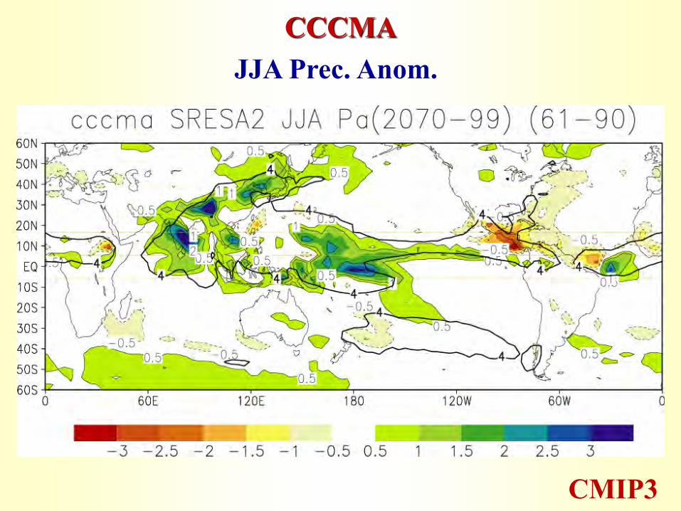
CCCMA JJA Prec. Anom.

CMIP3

CNRM_CM3 JJA Prec. Anom.

CMIP3

CSIRO_MK3 JJA Prec. Anom.

CMIP3

GFDL_CM2.0 JJA Prec. Anom.

CMIP3

GFDL_CM2.1 JJA Prec. Anom.

CMIP3

UKMO_HadCM3 JJA Prec. Anom.

CMIP3

MIROC_3.2 JJA Prec. Anom.

CMIP3

MRI_CGCM2 JJA Prec. Anom.

CMIP3

NCAR_PCM1 JJA Prec. Anom.

CMIP3

MPI_ECHAM5 JJA Prec. Anom.

CMIP3

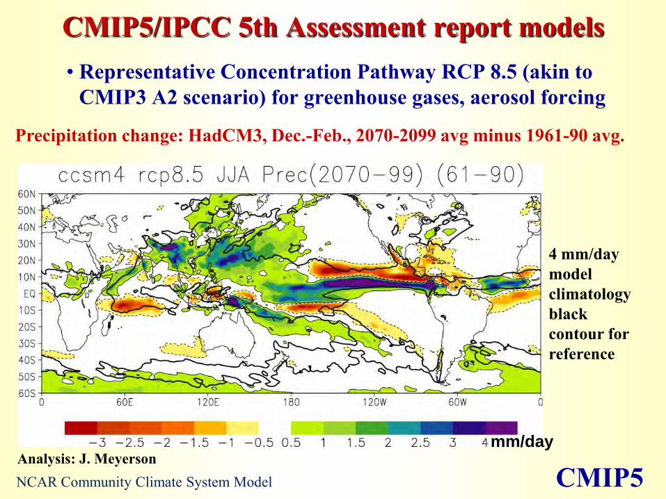
CMIP5/IPCC 5th Assessment report models • Representative Concentration Pathway RCP 8.5 (akin to

CMIP3 A2 scenario) for greenhouse gases, aerosol forcing

Precipitation change: HadCM3, Dec.-Feb., 2070-2099 avg minus 1961-90 avg.

4 mm/day model climatology black contour for reference

Analysis: J. Meyerson mm/day

CMIP5 NCAR Community Climate System Model

BCC-ESM1-1 JJA Prec. Anom.

CMIP5 Beijing Climate Center, China

CanESM2 JJA Prec. Anom.

CMIP5 Canadian Center for Climate Modelling and Analysis, Canada.

CCSM4 JJA Prec. Anom.

CMIP5 NCAR Community Climate System Model

CNRM-CM5 JJA Prec. Anom.

CMIP5 Centre National de Recherches Mereorologiques/ Centre Europeen de Recherche et Formation Avancees en Calcul Scientifique, France.

CSIRO-MK3 JJA Prec. Anom.

CMIP5 Commonwealth Scientific and Industrial Research Organization, Aus.

GISS-E2-R JJA Prec. Anom.

CMIP5 Goddard Institute for Space Studies

INMCM4 JJA Prec. Anom.

CMIP5 Institute for Numerical Mathematics, Russia.

IPSL-CM5A JJA Prec. Anom.

CMIP5 Institut Pierre Simon Laplace, France.

MRI-CGCM3 JJA Prec. Anom.

CMIP5 Meteorological Research Institute, Japan

NORESM1-M JJA Prec. Anom.

CMIP5 Norwegian Climate Center, Norway

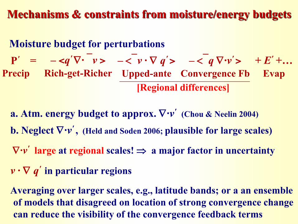
Mechanisms & constraints from moisture/energy budgets

Moisture budget for perturbations

0. At global scale neglect transport P' E', set by surface energy balance small increase (e.g., Allen & Ingram 2002,…)

0.1 Warmer temperatures & Clausius-Clapeyron q' tends to increase [Interplay with convection and dynamics q' ]

<>= vertical average; q' specific humidity; ' denotes changes

P' = – <`v · q' >Upped-ante

– <`q ·v' >Convergence Fb

+ E' +… Evap

– <q' · `v >Rich-get-Richer Precip

Mechanisms & constraints from moisture/energy budgets

“Rich-get-richer mechanism*”

Subtropics: low-level divergence

so q' increase Precip decrease

Convergence zones: vice versa

*(a.k.a. thermodynamic component):

Subtropics

Convergence zones

Moisture budget for perturbations P' = – <`v · q' >

Upped-ante – <`q ·v' >

Convergence Fb + E' +…

Evap – <q' · `v >

Rich-get-Richer Precip

Center of convergence zone: incr. moisture

convergence incr. precip

The Rich-get-richer mechanism

Chou & Neelin, 2004, Held & Soden 2006, Chou et al 2008

Descent region: incr. moisture divergence; less

often meets conv. threshold

Mechanisms & constraints from moisture/energy budgets

a. Atm. energy budget to approx. ·v' (Chou & Neelin 2004)

b. Neglect ·v' , (Held and Soden 2006; plausible for large scales)

·v' large at regional scales! a major factor in uncertainty

v · q' in particular regions

Averaging over larger scales, e.g., latitude bands; or a an ensemble of models that disagreed on location of strong convergence change can reduce the visibility of the convergence feedback terms

[Regional differences]

Moisture budget for perturbations P' = – <`v · q' >

Upped-ante – <`q ·v' >

Convergence Fb + E' +…

Evap – <q' · `v >

Rich-get-Richer Precip

West Coast rainfall change under global warming

CMIP5

DJF Prec. Anom. (2070-99)- (1961-90), RCP 8.5 scenario

Analysis: J. Meyerson

DJF Prec. Anom. CanESM2

CMIP5

DJF Prec. Anom. CCSM4

CMIP5

DJF Prec. Anom. CNRM-CM5

CMIP5

DJF Prec. Anom. CSIRO-MK3

CMIP5

DJF Prec. Anom. GISS-E2-R

CMIP5

DJF Prec. Anom. INMCM4

CMIP5

DJF Prec. Anom. IPSL-CM5A

CMIP5

DJF Prec. Anom. MRI-CGCM3

CMIP5

DJF Prec. Anom. NORESM1-m

CMIP5

How do the models do for El Niño/Southern Oscillation (ENSO)?

• A phenomenon we can observe

• Important for interannual prediction

• Satellite precipitation retrievals since 1979 • Atmospheric model component runs with observed sea

surface temperature (SST) or ocean atmosphere models • Rank correlation/Regression/compositing of events based on

an equatorial Eastern Pacific SST index “Nino3.4”

ENSO teleconnections to regional precip. anomalies

Su & Neelin, 2002 See Newell and Weare (1976); Salby & Garcia 1987; Yulaeva & Wallace (1994); Wallace et al.

(1998); Chiang and Sobel (2002); Kumar & Hoerling (2003); Su and Neelin 2003; Sperber and Palmer 1996, Giannini et al 2001; Saravanan & Chang, 2000; Joseph & Nigam 2006,…

Tropospheric temperature anomaly

Observed Nino3.4 rank correlations (Dec.-Feb.) CMAP

CPC Merged Analysis of Precipitation

Compare to preliminary results from CMIP5 models Analysis: B. Langenbrunner

CMIP5 models nino3.4 rank corr. AMIP runs(Dec.-Feb.) CanAM4

Canadian Center for Climate Modelling and Analysis, Canada.

CMIP5

CMIP5 models nino3.4 rank corr. AMIP runs(Dec.-Feb.) CCSM4

NCAR Community Climate System Model

CMIP5

CMIP5 models nino3.4 rank corr. AMIP runs(Dec.-Feb.) CNRM

Centre National de Recherches Mereorologiques/ Centre Europeen de Recherche et Formation Avancees en Calcul Scientifique, France.

CMIP5

CMIP5 models nino3.4 rank corr. AMIP runs(Dec.-Feb.) CSIRO

Commonwealth Scientific and Industrial Research Organization, Aus.

CMIP5

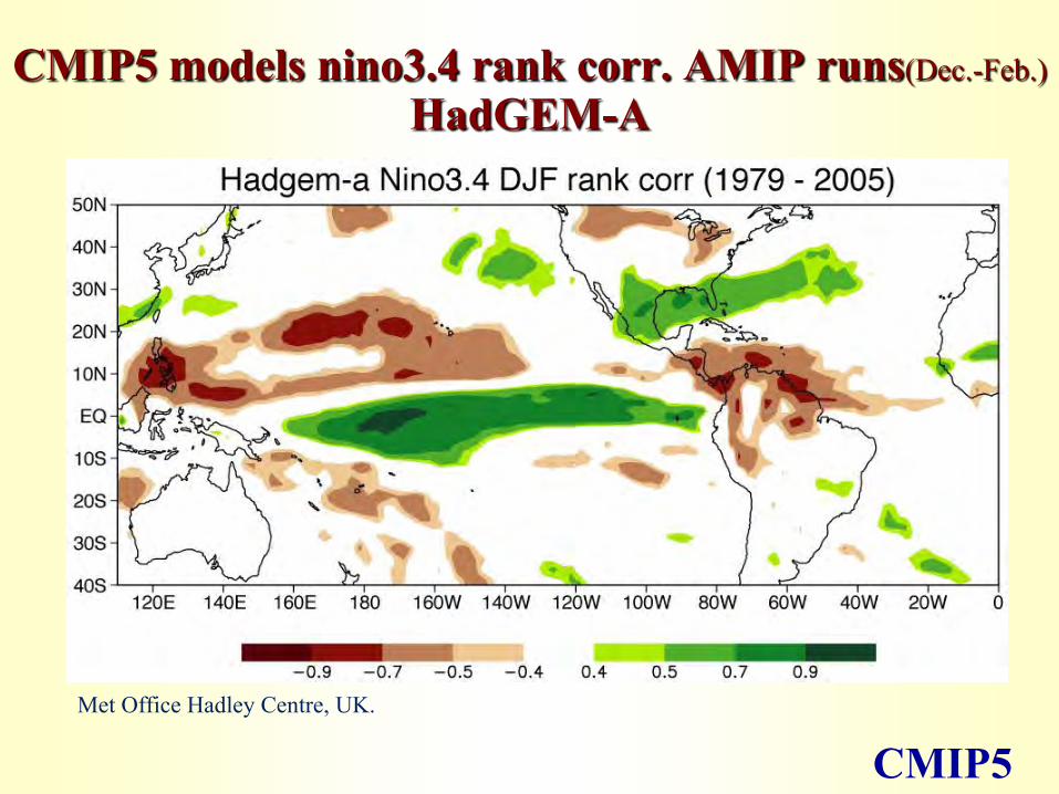
CMIP5 models nino3.4 rank corr. AMIP runs(Dec.-Feb.) HadGEM-A

Met Office Hadley Centre, UK.

CMIP5

CMIP5 models nino3.4 rank corr. AMIP runs(Dec.-Feb.) INMCM4

Institute for Numerical Mathematics, Russia.

CMIP5

CMIP5 models nino3.4 rank corr. AMIP runs(Dec.-Feb.) IPSL

Institut Pierre Simon Laplace, France.

CMIP5

CMIP5 models nino3.4 rank corr. AMIP runs(Dec.-Feb.) MPI

Max Plank Institute, Germany

CMIP5

CMIP5 models nino3.4 rank corr. AMIP runs(Dec.-Feb.) MRI

Meteorological Research Institute, Japan

CMIP5

CMIP5 models nino3.4 rank corr. AMIP runs(Dec.-Feb.) NorESM1-m

Norwegian Climate Center, Norway

CMIP5 Analysis: B. Langenbrunner

What is being done across the field?

• Higher-resolution models… (no guarantee) • Regional models (boundary conditions from global models) • Multimodel ensemble means and general (vs. regional) statements

• Large satellite data sets, field campaigns, monitoring at Atmospheric Radiation Measurement sites….

• Need to digest in ways that better constrain parameterizations* of moist convection at short time scales

• Understanding of parameter sensitivity/uncertainty quantification; practical means of optimizing models with available data

• Alternatives to point by point multi-model ensemble mean

*Parameterization: representation of bulk effects of small-scale phenomenon as a function of grid-scale variables

Hypothesis for disagreement on regional scale:

• models have similar processes for precip increases and decreases but the geographic location is sensitive …to differences in model clim. of wind, precip; convective closure (e.g. threshold)…

• agreement on amplitude measure* • suggests strong regional changes are likely that are not reflected in multi-model averages.

*e.g., spatial projection of precip change on each model’s own characteristic pattern

E.g., amplitude of precip incr/decr pattern shows

better agreement

Neelin, Munnich, Su, Meyerson and Holloway , 2006, PNAS

Projection of Jun-Aug (30yr running mean) precip pattern onto normalized positive & negative late-century pattern for each model

CMIP3

Despite disagreement on precise location, seek measures of extent of precip change that are more predictable

Integrated measures of regional precip. change cont’d

Analysis: B. Langenbrunner ; five year running mean shown for graphical clarity

Fraction of the globe with annual precipitation that would be in highest 5% (~20 year wet spell) during base period (1961-1990) for each model

CMIP5

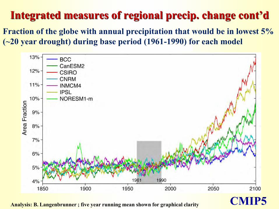
Integrated measures of regional precip. change cont’d

Analysis: B. Langenbrunner ; five year running mean shown for graphical clarity

Fraction of the globe with annual precipitation that would be in lowest 5% (~20 year drought) during base period (1961-1990) for each model

CMIP5

Are there fundamental considerations in climate model sensitivity that techniques

borrowed from optimization methods can help with?

Neelin, Bracco, Luo, McWilliams, Meyerson, 2010, PNAS.

• Precipitation parameter sensitivity a critical limitation to confidence levels in regional scale projections---arguably more important for impacts this century than climate sensitivity for global average temperature

• How nonlinear is this sensitivity? E.g., convection has sharp threshold for onset, but climate avgs over many instances

• Can we infer implications for the model improvement process and the use of multi-model ensemble averages to estimate projected precipitation changes?

Precipitation sensitivity cont’d

• Interest in systematic parameter sensitivity (esp. global avg climate sensitivity) and optimization in climate models (Severijns & Hazeleger 2005 Clim. Dyn., Stainforth et al. 2005 Nat., Jones et al. 2005 Clim. Dyn., Knight et al. 2007 PNAS, Kunz et al. 2007 Clim. Dyn., Jackson et al. 2008 J. Clim., Rougier et al. 2009 J. Clim.,…)

• # parameters N can easily be >10; a priori feasible range • Brute force sampling at density s gives order sN problem, but

e.g. ~N2 depending on nature of parameter dependence. Rough/smooth? High-order nonlin? Irreducible imprecision? • Here examined in the ICTP climate model

*International Centre for Theoretical Physics atmospheric general circulation model: ICTP AGCM; Molteni F., 2003, Climate Dyn.; Bracco et al. 2004, Climate Dyn.)

• Eight Sigma-levels, spectral triangular truncation T30 ~3.75 x 3.75-degree

Parameter dependence of RMS error* of June-Aug. precip as a function of cloud albedo, convective rel. hum., RHconv

AGCM ensemble mean over 10*25-year runs, (with observed sea surface temp.). Vertical size of symbol=2*standard error of ensemble mean Individual ensemble members shown for RHconv

*(vs. NCEP reanalysis) Neelin, Bracco, Luo, McWilliams, Meyerson, 2010, PNAS.

Try quadratic metamodel on space of N parameters μi for field j Simple but important: linear coefficient ai(x,t) & quadratic coefficient bij(x,t) are spatial & seasonal fields •e.g. of entry-level strategy for “computationally-expensive black-box functions” (cf. review by Shan & Wang, 2010, Struct. Multidisc. Optim.) •j can be a climatological field, anomaly regression, or other statistic from model output. Adopt multi-objective approach (for each field). •Then construct objective function, e.g., rms error (or sq. error, spatial correlation…) with typically a spatial mean, jobs observed, jstd the GCM for standard parameters •First fit: ai(x,t), bii(x,t) from the 2N endpoints of the μi ranges (order N integrations even if add redundant points). •For off-diagonal bij=bji: order N2 (at least N(N-1)/2 simulations).

1 1

N N N

std i i ij i ji i j

a bj j

1 / 22

ij j

Metamodel fit to param. dependence of AGCM fields

RMS error of June-Aug. precipitation (vs. NCEP) as a function of cloud albedo, convective RH

AGCM ensemble average versus linear and quadratic metamodels. Note negative curvature for relative humidity, due to ~quadratic nonlinearity in spatial field. No interior minimum boundary solution in constrained optimization problem

Neelin et al. 2010.

RMS error of June-Aug. precipitation (vs. reanalysis) as a function of convective RH but AGCM coupled to a

mixed-layer (ML) ocean (preindustrial CO2)

•Same properties in coupled model AGCM-ML average (250 yrs) versus linear and quadratic metamodel. Negative curvature for relative humidity (assoc. with ~quadratic nonlinearity in param. dependence of spatial fields) as in specified SST case. Vertical size of symbol=2*standard error

Neelin, Bracco, Luo, McWilliams, Meyerson 2010, PNAS.

Role of high dimensional fields in improvement challenges

Illustrate with case* of objective function f, (e.g. RMS precip error) with standard case error jerr μi f = gi + Aiiμi = 0 gi = 2aijerr, Aii = 2(ai

2 +2 biij) spatial average, metamodel linear coeff ai, quadratic bij. For simplicity neglect bij in curvature. μi = -aijerr/ ai

2If sensitivity ai had same spatial pattern as the standard case error jerrjstdjobsthis would cancel the error. Instead, compromise between reducing jerr and introducing new error.

Common experience: One region improves but another gets worse!

*case of interior minimum for diagonally dominant Hessian A

Parameter dependence for precipitation (etc) changes under global warming:

Implications for multi-model ensemble average • Does sensitivity across the feasible parameter domain

provide a prototype for differences among models? • If so, multi-model ensemble average ~ random sampling • If parameter dependence is linear, and distribution of

sample points is unbiased with respect to “true” parameter value multi-model ensemble average should work well

• parameter directions with (1) strong nonlinearity or (2) boundary optima (suggesting sampling across feasible range likely biased) can limit usefulness of multi-model ensemble average; e.g., convective rel. humidity param.

RMS difference (vs. Rhconv=0.9) of June-Aug. precipitation change as a function of convective RH for AGCM-ML

2xCO2 minus preindustrial CO2 AGCM ensemble average versus linear and quadratic fit. Note negative curvature for relative humidity, due to quadratic effects.

Neelin, Bracco, Luo, McWilliams, Meyerson 2010, PNAS.

Global warming precipitation change parameter dependence

Global warming precipitation change parameter sensitivity Ensemble-mean JJA precipitation (as a departure from the annual mean) for Conv. rel. hum. param max relative to the standard case for AGCM coupled to a mixed-layer ocean: change for 2xCO2 minus pre-industrial.

Linear contribution

Nonlinear contribution

Neelin, Bracco, Luo, McWilliams, Meyerson 2010, PNAS.

Implications for multi-model ensemble average

Column integrated water vapor ─ observational estimate from microwave retrievals*

*Satellite instruments: AMSR-E, SSMI; dynamic interpolation Wimmers & Velden (2007); footprint of input ~15 km; swath width ~1400 km; retrieval algorithm Alishouse et al. (1990)

Back to fundamentals: better constraining and

representing processes at small time/space scales

Column water vapor from NCAR CAM4* at 0.125 resolution

*National Center for Atmospheric Research Community Atmosphere Model, HOMME spectral

element dynamical core. Courtesy Mark Taylor (Sandia NL) & Rich Neale (NCAR).

Precipitation binned by column water vapor, w

• buoyancy & precip. pickup at high w

• Entraining convective available potential energy (CAPE) can match onset---if include enough turbulent entrainment into convecting parcel

• w useful because lots of microwave data available…

Neelin, Peters, Lin, Holloway & Hales, 2008, Phil Trans. Roy. Soc. A

An example of quantifying convective onset:

Transition to strong convection: Precip. dependence on tropospheric temperature & column water vapor

•Averages conditioned on vert. avg. temp. T, as well as w (T 200-1000mb from ERA40 reanalysis)

•Power law fits above critical: wc changes, same

•[note more data points at 270, 271]

^

• Analysed in tropics 20N-20S

Neelin, Peters & Hales, 2009 JAS

E. Pacific

Collapsed statistics for observed precipitation

• Precip. mean & variance dependence on w normalized by critical value wc; occurrence probability for precipitating points (for 4 T values); Event size distribution at Nauru

Tropospheric temperature T (k) T E. Pacific 269 270 x 271 272 p 273 274

^

Tropospheric temperature T (k) T E. Pacific 269 270 x 271 272 p 273 274

^

• Defines an empirical thermodynamic surface for the onset of strong convection to test models • Not a constant fraction of column saturation

Model

Obs

Transition to strong convection: High-resolution global model (CAM3.5, 0.5°) compared to observations (TMI)

Sahany et al. 2011, subm.

Model

Obs

Convective onset boundary

Transition to strong convection: High-resolution global model (CAM3.5, 0.5°) compared to observations (TMI)

Sahany et al. 2011, subm.

CAM3.5 entrainment

Low entrainment

Transition to strong convection: Obs. & model compared to simple convective plume instability

calculation with different entrainment assumptions

Obs

Low values of entrainment are inconsistent with observed onset

Transition to strong convection: simulation of current conditions

Community Climate System Model 4 (CAM4, 1°) Historical run 1981-2000

CAM4 Instantaneous precipitation data: R. Neale, Analysis K. Hales Column water vapor w (mm)

Conditionally avg. Precip P for bins of Tropospheric bulk temperature T (K)

Transition to strong convection: simulation under global warming

Community Climate System Model 4 (CAM4, 1°) Representative Concentration Pathway run RCP8.5 2081-2100

CAM4 Instantaneous precipitation data: R. Neale, Analysis K. Hales

Conditionally avg. Precip P for bins of Tropospheric bulk temperature T (K)

Column water vapor w (mm)

Importance of very small scales • Importance of entrainment to the onset of deep convection • Explains the high sensitivity to free tropospheric water

vapor (above the boundary layer) • Bad news: Beyond the resolution of global climate models

anytime soon (100m vs. 100 km) • Good news: work for cloud resolving modelers; new observations add constraints; revised model comes close • Bad news: interacts with other poorly constrained small scale processes cloud microphysics

Kirshbaum 2011

Outlook • The regional scale changes in the hydrological cycle are

arguably the most important aspect of climate sensitivity over the 21st century • Reducing regional uncertainty remains challenging with the current set of CMIP5 models---regions of agreement TBD

• Using climate model precipitation projections: Caution on simple statements; measure of uncertainty on multi-model ensemble mean; specific model validation for key phenomenon in the region of interest for each member of the ensemble

Outlook • The regional scale changes in the hydrological cycle are

arguably the most important… Will we do any better at reducing uncertainty?

Current tackling of small scale processes, scale interactions, new observational constraints, systematic parameter estimation methods,… seem likely to yield progress--- although not high precision by July 2012

Some connections… •Long tails seen in the probability distribution of water vapor also occur for chemical tracers including CO2: (B. Lintner, B. Tian, Q. Li, L. Zhang, P. Patra, M. Chahine) •And surface temperature (T. Ruff) •Simple stochastic model Fokker-Planck solutions indicate processes (S. Stechmann) •Nastier parameter dependence can occur (M. Chekroun et al.)

•Do constraints on entrainment combine with new proxy data to resolve a surface temperature vs. glacial elevation conundrum at last glacial maximum? (A. Tripati, S. Sahany, D. Pittmann, R. Eagle, J. Eiler, J. Mitchell, L. Beaufort)

• theory for inflow air mass interacting with convective onset at the margins of convection zones can be tested in models (H.Y. Ma, C.R. Mechoso, X. Ji)