Challenges in Deconvoluting Internal and Forced Climate Change Peter J. Webster School or Earth and Atmospheric Sciences Georgia Institute of Technology

Challenges in Deconvoluting Internal and Forced Climate Change

Peter J. WebsterSchool or Earth and Atmospheric Sciences

Georgia Institute of Technology

HADLEY GLOBAL SURFACE TEMPERATURE

B

C

D

A

E

F

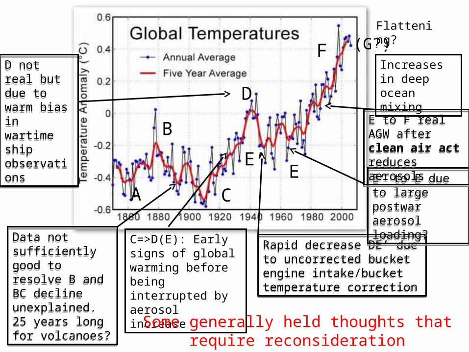
Peaks: Three peaks: B, D, F. Are all of these real or are the result of insufficient data or unresolved data biases

Valleys: Three valleys: A, C, E: Real or the result of data problems.

Transitions: Are the transitions the result of the same physical principles? E.g., Does decline B=>C differ in character from D=>E (or perhaps F=>G)? Ditto the inclines A=>B, C=>D and E=>F.

(G?)

B

C

D

AE

F (G?)

Important questions that we need to face are: Is global warming given by A => F (or G) or is curve a slow smaller trend superimposed large scale natural oscillations?

General tendency is to ignore bumps as data problems (uncorrected biases) or explain them as forced changes (e.g., anthropogenic aerosols). I have some problems with this.

B

C

D

AE

F (G?)

Rapid decrease DE’ due to uncorrected bucket engine intake/bucket temperature correction


E’E’ to E due to large postwar aerosol loading?

E’ to E due to large postwar aerosol loading?

E to F real AGW after clean air act reduces aerosols


D not real but due to warm bias in wartime ship observations


Data not sufficiently good to resolve B and BC decline unexplained. 25 years long for volcanoes?


Flattening?

Increases in deep ocean mixing

C=>D(E): Early signs of global warming before being interrupted by aerosol increase

Some generally held thoughts that require reconsideration

B

C

D

A

E

F (G?)



E’E’ to E due to large postwar aerosol loading?

E’ to E due to large postwar aerosol loading?







Flattening?

Increases in deep ocean mixing?

C=>D(E): Early signs of global warming before being interrupted by aerosol increase

Issues considered in this talk

(1) THE INCLINE FROM D TO E

C

D

Polyakov et al 2003

Polyakov et al. found SAT 1920-19450 variability of similar magnitude to recent warming. Also coupled dynamically coupled to MSLP.

IPCC AR4: A slightly longer warm period, almost as warm as the present, was observed from the late 1920s to the early 1950s (Polyakov et al 2003) . Although data coverage was limited in the first half of the 20th century, the spatial pattern of the earlier warm period appears to have been different from that of the current warmth

DYNAMICAL MODES AND ARCTIC TEMPERATURE

• The Arctic temperature correlates strongly with dynamical modes.• Critical that models get the physics of these modes for the correct

physical reasons• Warming in the Arctic is also manifested globally in the mid-1930’s

to 1945 …….

(2) Global temperature warming 1935-1945 (point D)

D

• During the mid-1930’s until mid-1940’s, global temperatures increased. This “bump” has not been discussed in AR4 and has been generally dismissed in the literature for a variety of reasons

• Biases in the SST data because of warm-time conditions: warm bias because buckets taken into warm cabins (for safety) for SST measurement.

• Lack of trained personnel making observations during wartime:

But, warming commenced well before WW2

• Previous incline due to global warming but SST bias at end of WW2 due to change from buckets to engine intake. (Thompson & Wallace 2007)

But, land temperatures also has a “synchronous”

bump where there are no buckets and engines

A comparison of station data with surrounding SST (NOAA)

Station data courtesy of P. Jones (CRU)

0.35C

Australia Pacific Ocean

0.25C

0.25C

North Pacific South Pacific


0.25C

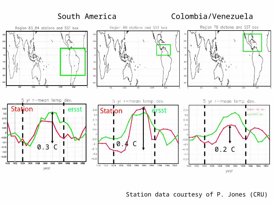
South America Colombia/Venezuela Central America

0.3 C 0.4 C0.2 C


Indian subcontinent Southeast Africa

0.35 C

0.45 C


• The 1930-40 bump is near global at least in the tropical strip from 40N/S where we analyzed the data

• The 1930/40 bumps is real and cannot be attributed to uncorrected SST measurements existing with near equal amplitude and phase (maybe: see later)

• But how good is the SST data used?

Summary: Land Station Data

(3) Transition/decline E’=>E

EE’

SH cooling >> NH cooling during E’ => E

• Recent SH optical depth< NH. From 1945-1970, difference probably greater. Improbable aerosol cooling!

• 1945 a previous unforced “hiatus” period?

(4) Recent “hiatus” F => G(?) GF

+0.5

0

CRU

1980 2000

• Two recent studies (Katsman and van Oldenborgh, 2011, and Meehl et al, 2011) have noted reduced heating of upper ocean and enhanced downward heat transport to deep ocean during periods of constant surface temperature

• These referred to as hiatus periods and are model results. Observations not sensitive enough to test.

F G

Changes in heat flux hiatus versus non-hiatus decades

Impacts of changes in deep ocean mixing

• During a hiatus period, 1 Wm-2 mixed to greater depths (Meehl et al. 2011)

• What happens to the heat mixed to deeper ocean?

• It is uncertain if episodic deep mixing is an important process. But it may explain long periods of constant temperature/cooling such as between 1945-70

• Clearly, there is a strong need to understand ocean processes to a far greater degree.

• In NCAR press release and in subsequent discussion it was argued that:

“…this heat will come back to haunt us… It is a matter of conservation of energy…”

Is this true? Will the heat become available to the atmosphere at a later time: the “double whammy”?

• Energy is conserved but the Second Law of Thermodynamics precludes the “haunting” or a return of the heat?

• Mixing, marked by an increase in entropy, is an irreversible process. The deeply mixed heat becomes unavailable for further atmospheric heating!

BUT, WHAT ABOUT THE SST DATA?

• Comparison of the land data and the SST data shows that the 1930-1940 bump was real.

• Land and ocean temperatures appear in phase but there are some intriguing phase differences (real?)

• But how good are the consolidated SST data sets? Are they sufficiently accurate to determine the major indices such as the AMO, PDO and etc.

• To consider this issue we compare actual ship observations with reconstructed SST data sets

• Sea-surface temperature anomaly fields, such as these, exist back to 1870, even though there were periods when there was very little data (see Allan et al. 2005).

• How are these computed and how can we check their fidelity?

SST Anomaly

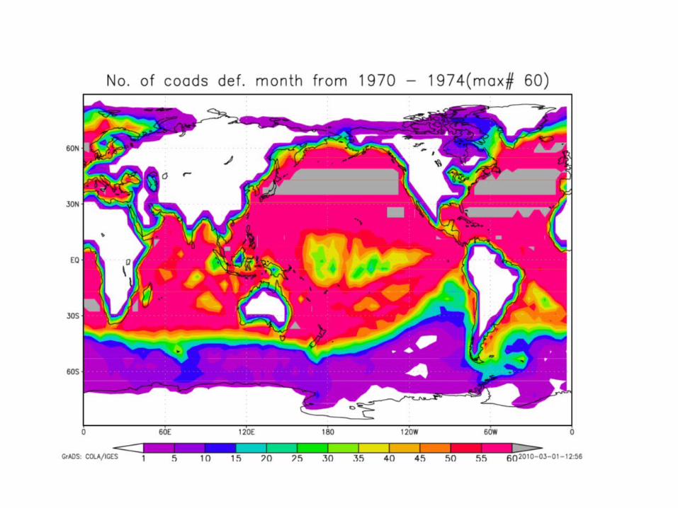
ICOADS 1920-24 Regions of high data density:ICOADS data collected to provide first estimate of SST

Regions of low data density:Filled with gridded data (or EOFs) determined from modern data.Hadley uses 1960-90 mean

Overall field of SST for particularperiod determined using an interpolation technique.

Anomaly field determined by subtracting arbitrary gridded mean field

One test of such schemes would be to compare the actual ICOADS data with the final anomaly product. Is information lost or gained? Do the anomalies match?

1920-24

To perform the test, we choose areas where there is a high density of ICOADS data

ABC

DE

FG

H

IJKL

M NO

N

P

X

Y

NORTH ATLANTIC

AB

C

A

B

C

ersst: Hadley:ICOADS:

EQUATORIAL & SOUTH ATLANTIC

DE

M

D

E

Mersst: Hadley:ICOADS:

NORTH INDIAN OCEAN

K JL

K

J

Lersst: Hadley:ICOADS:

NW PACIFIC

GH

P

G

H

P


SOUTHWEST AUSTRALIA

NO

N

O


General summary: reconstructions tend to reduce amplitude of base data variability.

N

To illustrate how different the assessments of surface temperature are….

N

X

Y

X Y

SIMPLE CONCLUSION AND A “TEASER”

• Clear to me that IPCC didn’t consider earlier excursions < 1970• Need to understand long-term ocean-atmosphere (-land) interactions to

understand climate change• Without an a priori theory of the complete system (forced and internal)

we are bound to a path of the extrapolation of poor data and a belief in incomplete models.

And, there may be some surprises as we seek this understanding:

Detrended Correlation: -0.82

Net ocean heating

Net ocean heating

Very strong anti-correlation between net ocean heating and net land heating 20oN-20oS. Occurs in all reanalyses.

NCEP reanalysis

Documents

Challenges in Deconvoluting Internal and Forced Climate Change Peter J. Webster School or Earth and Atmospheric Sciences Georgia Institute of Technology