ChainingThis exposition was developed by Clemens Gropl. It is based on the following refer-ences, which are all suggested reading:

• Mohamed I. Abouelhoda, Enno Ohlebusch: Chaining algorithms for multi-ple genome comparison, Journal of Discrete Algorithms, 3:321-341, 2005.[AO05]

• Enno Ohlebusch, Mohamed I. Abouelhoda: Chaining algorithms and applica-tions in comparative genomics, Handbook of Computational Molecular Biology,Chapter 15, 2006. [AO06]

• Gene Myers, Webb Miller: Chaining multiple-alignment fragments in sub-quadratic time, SODA 1995. [MM95]

The work of Ohlebusch and Abouelhoda was originally presented in two conferencepapers at CPM03 and WABI03. These are now mostly superseded by the twoarticles above.

12000

The chaining problem

Biological sequence analysis often has to deal with sequences of genomic sizewhich cannot be aligned as a whole in one step. In this situation, an anchor-basedapproach can be used. The idea is to construct a (more or less) global alignmentfrom a collection of local alignments. The small pieces are also called fragmentmatches or just fragments. These pieces then have to be chained one after another.The chaining problem is difficult because no all fragment are compatible with eachother. The general approach is as follows:

1. Compute fragments, i. e. regions in the genomes that are very similar.

2. Compute an optimal global chain of colinear non-overlapping fragments. Thefragments of the chain are the anchors for the alignment.

3. Fill in the gaps by aligning the regions between the anchors.

A variant of the problem (2’.) tries to find a set of local chains instead of one globalchain. We will return to this later.

12001

The chaining problem (2)

Naturally we are also interested in multiple alignments of k genomic sequences. Forthe chaining problem, we only care about where each fragment begins and ends ineach of the k sequences.

Each fragment has a weight . The weight could be the length of an exact match, oranother measure of its statistical significance.

The gaps in a chain of fragments need to be scored as well. We will see a numberof scoring schemes for this below.

12002

The chaining problem (3)

Example. To the left, you see a collection of pairwise (k = 2) alignments (top)and a chained subset of them (bottom). To the right you see a two-dimensionalvisualization of the same fragment matches. An arrow indicates that one fragmentcan follow another fragment in a chain. (Not all possible arrows are shown.)

12003

The chaining problem

Note that not all pairs of fragments are compatible to each other: The fragments inthe chain have to be collinear and non-overlapping.

• Collinear : The order of the respective segments of the fragments is the samein both sequences.

• Non-overlapping: Two fragments overlap if their segments overlap in one of thesequences.

In the pictorial representation of Figure (a), two fragments are collinear if the linesconnecting their segments are non-crossing (for example, the fragments 2 and 3are collinear, while 1 and 6 are not). Two fragments overlap if their segments over-lap in one of the genomes (for example, the fragments 1 and 2 are overlapping,while 2 and 3 are non-overlapping). Figure (b) shows the fragments as rectangles.Fragments 2, 3, 7 are chained. 0 and t are artificial source and sink nodes.

12004

The chaining problem (2)

Among the many bioinformatics tools solving chaining problems (in some way) are:

• FastA. Fragments are constant-size exact matches. They are found by hashing.

• MUMmer . Fragments are maximal exact matches. They are found using suffixtrees.

• MGA. Fragments are maximal multiple exact matches. They are found usingsuffix arrays.

• GLASS. Fragments are exact k-mers.

• DIALIGN. Fragments can have substitutions.

• MultiPipMaker . Fragments can have substitutions and indels.

• . . . (add your favorite genome alignment tool here)

The fragments could also be BLAST hits, or even local chains from an earlier invo-cation of the algorithm.

12005

Graph-theoretic formulation

Clearly the chaining problem can be stated in graph-theoretic terms. The fragmentscorrespond to vertices and we have an edge whenever two fragments are com-patible, i. e. they can be combined in a chain. Thus we obtain a weighted acyclicdirected graph. The goal is to find a directed path of maximum weight. A simpledynamic programming requires O(V + E) time and space.

12006

Graph-theoretic formulation (2)

Example.

· · · · · · · · · · · · · · · · · · · · ·· i · · · · · · · · · · · · · · · · · · ·· · i · · · · g · · · · · · · · · · · · ·· · · · · · · · g · · · · · · · · · · · ·· · · · · · · · · g · · · · · · · · · · ·· · · · · · d · · · · · a · · · · · · · ·· · c · · · · d · · · · · a · · · · · · ·· · · c · · · · · · · · · · a · · · · · ·· · · · · · · · · · · h · · · a · · · · ·· · · · · k · · · · · · h · · · · · · · ·· b · · · · k · · · · · · h · · · · · · ·· · b · · · · · · · f · · · h · · · · · ·· · · b · · · · · · · f · · · · · j · · ·· · · · b · · · · · · · f · · e · · j · ·· · · · · b · · · · · · · · · · e · · j ·· · · · · · b · · · · · · · · · · · · · ·· · · · · · · · · · · · · · · · · · · · ·

a / 8

j / 6

-3

b / 12c / 4

h / 8

-7k / 4

-1

d / 4

f / 6

-4 -3

e / 4

g / 6

-2 -6 -3

-1-2

i / 4

-3

-3

Scoring scheme: For simplicity, each “letter” scores 2 and all other columns of thecorresponding alignment score −1 (diagonal “shortcuts” are allowed).

12007

Graph-theoretic formulation (3)

The graph theoretic approach is intuitive and will lead us to the final solution. Butsome essential issues are not settled yet:

• How should the edge set be constructed? Of course we can enumerate overall pairs of vertices, but this will take Ω(V 2) time, which is prohibitive in manyreal-world cases.

• Even worse, it is easy to construct instances where the size of the edge set isindeed Ω(V 2). It may help to remove “transitive” edges which cannot be partof an optimal solution, but this does not improve the worst-case asymptotic.(Exercise: find such an example.)

• The obvious dynamic programming algorithm does not fully exploit the geomet-ric nature of the problem. It works on every weighted acyclic directed graph,but our graph is more restricted.

The good news is that we need not construct the edge set explicitly . Instead we willtraverse the vertices in an appropriate order and use some auxiliary data structuresand still carry out essentially the same DP recursion.

12008

Notation

Before we can get more concrete, we need to introduce some notation.

• For 1 ≤ i ≤ k , let Si = Si [1..ni ] be a sequence of length |Si | = ni .

• Si [l ..h] denotes the substring of Si starting at position l and ending at positionh. (Both margins are included.)

• A fragment f consists of two k -tuples beg(f ) = (l1, l2, ... , lk ) and end(f ) =(h1, h2, ... , hk ) such that the strings S1[l1..h1], S2[l2..h2],. . . ,Sk [lk ..hk ] are simi-lar in some sense.

• A fragment f of k sequences can be represented by a hyper-rectangle inRk with two extremal corner points beg(f ) and end(f ). We write R(p, q) :=[p1, q1] × ... × [pk , qk ] for the hyper-rectangle spanned by p = (p1, ... , pk ) andq = (q1, ... , qk ), where p < q, i. e., pi < qi for all 1 ≤ i ≤ k . Thus a fragmentf is represented by hyper-rectangle R(beg(f ), end(f )). Each coordinate of thecorners is a nonnegative integer.

• Consequently, the number of sequences k is also called the dimension.12009

Notation (2)

• Each fragment f has a weight f .weight ∈ R.

• We will sometimes identify beg(f ) or end(f ) with f .

• For ease of presentation, we introduce artificial fragments of weight zero. Welet 0 := (0, ... , 0) and t := (n1+1, ... , nk +1). We let beg(0) := ⊥ (where⊥means“undefined”) and end(0) := (0, ... , 0). Analogously, beg(t) := (n1 + 1, ... , nk + 1)and end(t) := ⊥.

• The coordinates of a point p ∈ Rk will be accessed as p.x1,. . . ,p.xk . If k = 2,we will also write them as p.x , p.y .

12010

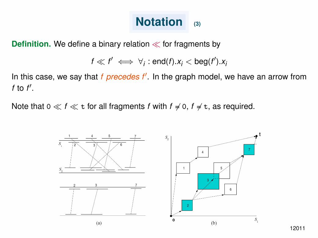
Notation (3)

Definition. We define a binary relation for fragments by

f f ′ ⇐⇒ ∀i : end(f ).xi < beg(f ′).xi

In this case, we say that f precedes f ′. In the graph model, we have an arrow fromf to f ′.

Note that 0 f t for all fragments f with f 6= 0, f 6= t, as required.

12011

Notation

Definition.

• A chain (of collinear, non-crossing fragments) is a sequence of fragments C =(f1, ... , f`) such that fi fi+1 for all 1 ≤ i < `.

• The score of C is

score(C) :=∑i=1

fi .weight−`−1∑i=1

g(fi+1, fi) ,

where g(fi+1, fi) is the gap cost for connecting fragment fi to fi+1 in the chain.

The global fragment chaining problem is:

Given a set of weighted fragments and a gap cost function, determine achain of maximum score starting at 0 and ending at t.

12012

The basic algorithm

For each fragment f , denote by f .score the maximum score of all chains starting at0 and ending at f .

Clearly this score satisfies the following recurrence:

f ′.score = f ′.weight + max

f .score− g(f ′, f )∣∣ f f ′

.

The simple dynamic programming algorithm for the global fragment chaining prob-lem processes the fragments in a topological ordering (e. g., the lexicographic or-dering). This is to ensure that when f ′.score is going to be computed, all valuesf .score, where f f ′, have already been determined.

The initialization is

0.score := 0 .

And the value we are finally interested in is t.score.

The chain itself can be found by backtracing, as usual.

12013

Range maximum queries

So how are we going to improve upon this straightforward solution? The key isto compute the ‘max’ in the DP recursion more efficiently, without ‘generating’ allthe edges of the graph. Range (maximum) queries are a fundamental operation incomputational geometry, and efficient data structures have been designed for them.

12014

Range maximum queries (2)

Definition.

• Let S ⊆ Rk be a set of points and let p, q ∈ Rk , p < q be the corners of arectangle R(p, q). Then the range query RQ(p, q) asks for all points of S thatlie in the hyper-rectangle R(p, q).

• Assume further that the points in S have a score associated with them. Thenthe range maximum query RMQ(p, q) asks for a point of maximum score inR(p, q).

Observation. Consider the special case when the gap cost function g is alwayszero. Let ~1 := (1, ... , 1). The recurrence of the basic algorithm implies:

If RMQ(0, beg(f ′)−~1) returns the end point of fragment f , then f ′.score = f ′.weight+f .score.

In other words, range maximum queries are what we need in the DP recursion!

12015

Global chaining without gap costs

In the following, we will first consider the case when all gap costs are zero. Afterthat we will see how the algorithm can be modified to deal with (certain) gap costfunctions.

The algorithm uses the line-sweep paradigm to construct an optimal chain. It pro-cesses the begin and end points of the fragments in ascending order of their x1coordinate. One can think of the traversal as a line (actually, a hyper-plane of di-mension k−1) that “sweeps” the points with respect to their x1 coordinate.∗ If a pointhas already been scanned by the sweeping line, it is said to be active, otherwise itis said to be inactive.

Let s be the point that is currently being scanned. The x1 coordinates of the activepoints are less than or equal to that of s. By the preceding observation, if s is thebegin of fragment f ′, then an optimal chain ending at f ′ can be found by a rangemaximum query over the active points. Otherwise, s is the end of a fragment andcan be activated . Note that the RMQ need not take the first coordinate x1 intoaccount because of the sweeping order.∗engl. “to sweep” = dt. “fegen”

12016

Global chaining without gap costs (2)

The algorithm uses a semi-dynamic data structure D that stores the end points ofthe fragments and supports two operations:

1. Activation

2. Range maximum queries over active points.

It is called semi-dynamic because we can only ‘activate’ but not ‘inactivate’ points.Abouelhoda and Ohlebusch [AO05] have designed such a data structure that sup-ports RMQs with activation in O(n logd−1 n log log n) time and O(n logd−1 n) spacefor n points in d dimensions.

Since d = k −1 in the algorithm, their algorithm solves the global fragment chainingproblem in O(n logk−2 n log log n) time and O(n logk−2 n) space. (This holds fork ≥ 3; for k = 2 the running time is dominated by the initial sorting.)

The correctness of the following algorithm is immediate.

12017

Global chaining without gap costs (3)

Algorithm. (k -dimensional chaining of n fragments)1 // Data structure D is (k − 1)-dimensional, x1 is ignored.2 // π denotes the projection.3 points := begin and end points of all fragments (including 0 and t)4 sort points by x15 store all end points of fragments as inactive in D6 for i = 1 to 2n + 2 do7 if points[i ] == beg(f ′) for some fragment f ′

8 then9 q := RMQ(0,π(points[i ]− ~1))

10 f := fragment with end(f ) == q and maximum score11 f ′.prec := f12 f ′.score := f ′.weight + f .score13 else // points[i ] == end(f ′) for some fragment f ′

14 activate(π(points[i ])) in D15 fi16 od

12018

Global chaining without gap costs (4)

The details of the data structure D are fairly complicated. It combines range treeswith fractional cascading and van Emde Boas priority queues (with Johnson’s im-provement) . . . enough topics for more than another lecture! We therefore skip thispart of [AO05, AO06] :-( Note that the actual implementation of Abouelhoda usesKD-trees, which are non-optimal with respect to the running times but much easierto implement. (Explained on the blackboard.)

At this point, we have an algorithm for the global chaining problem without gap costs.Next we show how to modify the algorithm to take certain gap cost functions intoaccount.

12019

Incorporating L1 gap costs

Definition. For two points p, q ∈ Rk , the L1 distance is defined by

d1(p, q) :=k∑

i=1|p.xi − q.xi | .

Definition. The L1 gap function is

g1(f ′, f ) := d1(beg(f ′), end(f )) for f f ′.

The effect of the L1 gap function is that all characters between f and f ′ are scoredas indels (not a very realistic assumption, but maybe not so bad either):

ACCXXXX---AGG

ACC----YYYAGG

In this example ACC and AGG are the anchors of the alignment and X and Y areanonymous characters.

12020

Incorporating L1 gap costs (2)

The problem with gap costs is that a range maximum query does not immediatelytake the gap cost g(f ′, f ) into account when f ′.score is computed.

But we can express the gap costs implicitly in terms of the weight information at-tached to the points. Let us define the geometric cost of a fragment f as

gc(f ) := d1(t, end(f )) .

Since t is fixed, the value gc(f ) is known in advance for every fragment f . Moreover,we have the following lemma:

Lemma 1. Let f , f , and f ′ be fragments such that f f ′ and f f ′. Then

f .score− g1(f ′, f ) > f .score− g1(f ′, f ) ⇐⇒ f .score− gc(f ) > f .score− gc(f ) .

Proof: Exercise. (See figure on blackboard.)

12021

Incorporating L1 gap costs (3)

Therefore we need only two slight modifications to the algorithm in order to take L1gap costs into account.

1. Replace the statement

f ′.score := f ′.weight + f .score

with

f ′.score := f ′.weight + f .score− g1(f ′, f ) .

2. If points[i ] is the end point of f ′, then it is activated with priority

f ′.priority := f ′.score− gc(f ′) .

Thus the RMQs will return a point of maximum priority instead of a point ofmaximum score.

12022

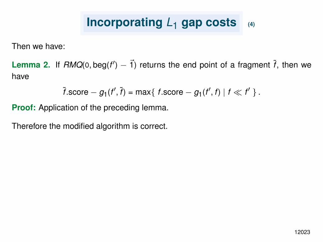
Incorporating L1 gap costs (4)

Then we have:

Lemma 2. If RMQ(0, beg(f ′) − ~1) returns the end point of a fragment f , then wehave

f .score− g1(f ′, f ) = max f .score− g1(f ′, f ) | f f ′ .

Proof: Application of the preceding lemma.

Therefore the modified algorithm is correct.

12023

Incorporating L1 gap costs (5)

Algorithm. (k -dimensional chaining of n fragments using L1 gap cost)1 // Data structure D is (k − 1)-dimensional, x1 is ignored.2 // π denotes the projection.3 points := begin and end points of all fragments (including 0 and t)4 sort points by x15 store all end points of fragments as inactive in D6 for i = 1 to 2n + 2 do7 if points[i ] == beg(f ′) for some fragment f ′

8 then9 q := RMQ(0,π(points[i ]− ~1))

10 f := fragment with end(f ) == q and maximum score11 f ′.prec := f12 f ′.score := f ′.weight + f .score− g1(f ′, f )13 else // points[i ] == end(f ′) for some fragment f ′

14 f ′.priority := f ′.score− gc(f ′)15 activate(π(points[i ])) in D with priority f ′.priority16 fi17 od

12024

Incorporating sum-of-pairs gap costs

The L1 gap cost model is not very realistic. An alternative scoring model was intro-duced by Myers and Miller [MM95]. We consider the case k = 2 first, since the casek > 2 is rather involved. (The name ‘sum-of-pairs cost’ is a bit misleading, just takeit as a name.)

12025

Incorporating sum-of-pairs gap costs (2)

For two points p, q ∈ Rk , we write

∆xi (p, q) := |p.xi − q.xi |

The sum-of-pairs distance depends on two parameters ε and λ. It is defined (fork = 2) as

d(p, q) :=

ε∆x2 + λ(∆x1 −∆x2) if ∆x1 ≥ ∆x2

ε∆x1 + λ(∆x2 −∆x1) if ∆x2 ≥ ∆x1

=

λ∆x1 + (ε− λ)∆x2 if ∆x1 ≥ ∆x2

λ∆x2 + (ε− λ)∆x1 if ∆x2 ≥ ∆x1 .

We drop the arguments p, q if they are clear from the context.

12026

Incorporating sum-of-pairs gap costs (3)

Definition. The sum-of-pairs gap function is

g(f ′, f ) := d(beg(f ′), end(f )) for f f ′.

The effect of the sum-of-pairs gap function depends on the parameters ε and λ.

• λ > 0 is the cost of aligning an anonymous character with a gap position in theother sequence.

• ε > 0 is the cost of aligning two anonymous characters to each other.

For λ = 1 and ε = 2, g coincides with g1, whereas for λ = 1 and ε = 1, we obtain theL∞ metric: g∞(f ′, f ) := d∞(beg(f ′), end(f )), where

d∞(p, q) = max |p.xi − q.xi | | 1 ≤ i ≤ k .

12027

Incorporating sum-of-pairs gap costs (4)

With λ > ε/2 > 0 the characters between two fragments are replaced as long aspossible and the remaining characters are inserted or deleted:

ACCXXXXAGG

ACCYYY-AGG

(Compare this example to the one for the L1 metric.)

Otherwise it would be best to connect fragments entirely by gaps as in the L1 metric.Thus we require that λ > ε/2.

12028

Incorporating sum-of-pairs gap costs (5)

We need a few definitions in order explain how the score of a fragment f ′ can becomputed.

Let s := beg(f ′). The first quadrant of s consists of all points p ∈ R2 with p.x1 ≤ q.x1and p.x2 ≤ q.x2.

We subdivide the first quadrant of s into its first and second octant O1, O2. Thepoints in the first octant O1 satisfy ∆x1 ≥ ∆x2; they are above or on the straight linex2 = x1 + (s.x2 − s.x1). The points in the second octant satisfy ∆x2 ≥ ∆x1.

Clearly,

f ′.score = f ′.weight + maxv1, v2 ,

where

vi := max f .score− g(f ′, f ) | f f ′ and end(f ) lies in octant Oi

for i = 1, 2. Thus we can eliminate the case distinction for g within each octant.

12029

Incorporating sum-of-pairs gap costs (6)

We are not finished yet, since our chaining algorithm relies on RMQs, which workfor orthogonal regions, not octants! But a simple trick can help.

We apply the octant-to-quadrant transformations of Guibas and Stolfi: The trans-formation T1 : (x1, x2) 7→ (x1 − x2, x2) maps the first octant to the first quadrant.Similarly, T2 : (x1, x2) 7→ (x1, x2− x1) does the same task for the second octant. Bymeans of these transformations, we can apply the same techniques as for the L1metric.

We only need to define the geometric cost gci properly for each octant Oi .

12030

Incorporating sum-of-pairs gap costs (7)

Lemma 3. Let f , f , and f ′ be fragments such that f f ′ and f f ′. If end(f ) andend(f ) lie in the first octant of beg(f ′), then

f .score− g(f ′, f ) > f .score− g(f ′, f ) ⇐⇒ f .score− gc1(f ) > f .score− gc1(f ) ,

where

gc1(f ) = λ∆x1(t, end(f )) + (ε− λ)∆x2(t, end(f ))

for any fragment f .

Proof: Exercise. (Similar to the preceding one.)

An analogous lemma holds for the second octant.

12031

Incorporating sum-of-pairs gap costs (8)

Due to the octant-to-quadrant transformations, we need to take two different geo-metric costs gc1, gc2 into account. Consequently, the nodes will also have differentscores with respect to both. To cope with this, we use two data structures D1, D2.Each Di stores the points of the set Ti(end(f )) | f is a fragment . The results ofboth RMQs need to be merged. We omit the details.

We still have a line-sweep algorithm, but the data structures Di need to storetwo-dimensional points. Thus the algorithm runs in O(n log n log log n) time andO(n log n) space.

12032

Incorporating sum-of-pairs gap costs (9)

For dimensions k > 2, the sum-of-pairs gap cost is defined for fragments f f ′ by

gsop(f ′, f ) :=∑

0≤i<j≤kg(f ′i ,j , fi ,j) ,

where f ′i ,j and fi ,j are the two-dimensional “projections” of the fragments.

The general idea is similar as for k = 2, but now the first hyper-corner of beg(f ′) issubdivided into k ! hyper-regions.

The resulting algorithm runs in O(k !n logk−1 n log log n) time and O(k !n logk−1 n)space.

12033

Local chaining

So far we have been searching for an optimal chain starting at 0 and ending at t. Ifwe remove the restriction that a chain must start at 0 and end at t, we obtain thelocal chaining problem.

Definition. The local fragment chaining problem is: Given a set of weighted frag-ments and a gap cost function, determine a chain of maximum score ≥ 0. Such achain will be called an optimal local chain.

12034

Local chaining (2)

Example:

The optimal chain is composed of the fragments 1, 4, and 6. Another significantlocal chain consists of the fragments 7 and 8.

12035

Local chaining (3)

Definition. Let

f ′.score := max score(C) | C is a chain ending with f ′

Definition. A chain C ending with f ′ and satisfying f ′.score = score(C) is called anoptimal chain ending with f ′.

We explain the idea using L1 gap costs for simplicity.

Lemma. The following equality holds:

f ′.score = f ′.weight + max 0, f .score− g1(f ′, f ) | f f ′ .

Once again we have switched from global to local alignment by ‘adding a zero atthe right place’.

Now the modification to the line-sweep algorithm is straight-forward.

12036

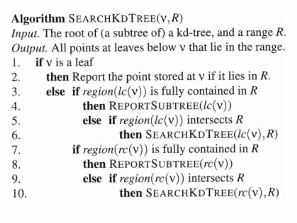
KD-trees

The actual implementation done by Abouelhoda uses a KD-tree data structure.

A nice Java applet illustrating KD-trees (for dimension k = 2) can be found viaHanan Samet’s homepage, http://www.cs.umd.edu/users/hjs/, the direct linkto the applet is http://donar.umiacs.umd.edu/quadtree/points/kdtree.html.This is the one I presented in the lecture, but it was offline on 2007-06-22, so I wenton to another one.

Another nice Java applet can be found via Huseyin Akcan’s homepage, http://cis.poly.edu/~hakcan01/, the direct link to the applet is http://cis.poly.edu/

~hakcan01/projects/kdtree/kdTree.html, and this is also where I have copiedthe pseudocode from.

12037

KD-trees (2)

12038

KD-trees (3)

12039

KD-trees (4)

12040

KD-trees (5)

12041

KD-trees (6)

12042

KD-trees (7)

12043

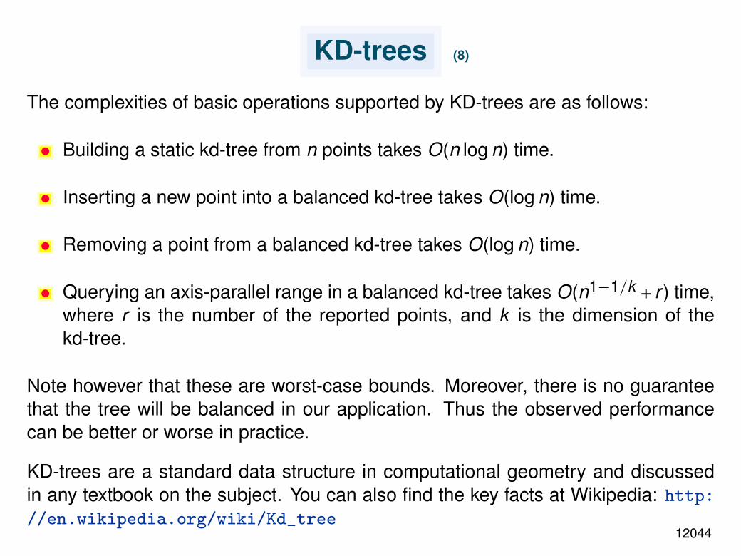
KD-trees (8)

The complexities of basic operations supported by KD-trees are as follows:

• Building a static kd-tree from n points takes O(n log n) time.

• Inserting a new point into a balanced kd-tree takes O(log n) time.

• Removing a point from a balanced kd-tree takes O(log n) time.

• Querying an axis-parallel range in a balanced kd-tree takes O(n1−1/k + r ) time,where r is the number of the reported points, and k is the dimension of thekd-tree.

Note however that these are worst-case bounds. Moreover, there is no guaranteethat the tree will be balanced in our application. Thus the observed performancecan be better or worse in practice.

KD-trees are a standard data structure in computational geometry and discussedin any textbook on the subject. You can also find the key facts at Wikipedia: http://en.wikipedia.org/wiki/Kd_tree

12044

Conclusion

12045