1

2

3

4

5

Teaching Tip: Modern economic growth only emerged in the most recent two or three centuries. For the second bullet, think of per capita GDP as a rough measure of standard of living.

One of the most important facts of economic growth is that sustained increases in standards of living are a remarkably recent phenomenon. Up until about 12,000 years ago, humans were hunters and gatherers, living a nomadic existence. Then around 10,000 BC. came an agricultural revolution, which led to the emergence of settlements and eventually cities. Yet even the sporadic peaks of economic achievement that followed were characterized by low average standards of living. Evidence suggests, for example, that wages in ancient Greece and Rome were approximately equal to wages in Britain in the fifteenth century or France in the seventeenth, periods distinctly prior to the emergence of modern economic growth.

6

Since 1700, however, living standards in the richest countries have risen from roughly $500 per person to something approaching $45,000 per person today. Incomes have exploded by a factor of 90 during a period that is but a flash in the pan of human history. If the 130,000-year period since modern humans made their first appearance were compressed into a single day, the era of modern growth would have begun only in the last 3 minutes. An important result of these differences in timing is that living standards around the world today vary dramatically. Per capita GDP in Japan and the United Kingdom is about 3/4 that in the United States; for Brazil and China, the ratio is 1/5, and for Ethiopia only 1/40. These differences are especially stunning when we consider that living standards around the world probably differed by no more than a factor of 2 or 3 before the year 1700. In the last three centuries, standards of living have diverged dramatically, a phenomenon that has been called the Great Divergence.

7

8

Graph of the “Great Divergence” Figure 3.1 makes this point by showing estimates of per capita GDP over the last 2,000 years for six countries. For most of history, standards of living were extremely low, not much different from that in Ethiopia today. The figure shows this going back for 2,000 years, but it is surely true going back even farther. Since 1700, living standards in the richest countries have risen from roughly $500 per person to something approaching $45,000 per person today. On a long time scale, economic growth is so recent that a plot of per capita GDP looks like a hockey stick, and the lines for different countries are hard to distinguish. Growth first starts to appear in the United Kingdom and then in the United States. Standards of living in Brazil and Japan begin to rise mainly in the last century or so, and in China only during the last several decades. Finally, standards of living in Ethiopia today are perhaps only twice as high as they were over most of history, and sustained growth is not especially evident.

Measured in year 2005 prices, per capita GDP in the United States was about $2,800 in 1870 and rose to more than $42,000 by 2009, almost a 15-fold increase. A more mundane way to appreciate this rate of change is to compare GDP in the year you were born with GDP in the year your parents were born. In 1990, for example, per capita income was just over $32,000. Thirty years earlier it was under $16,000. Assuming this economic growth continues, the typical American college student today will earn a lifetime income about twice that of his or her parents.

9

10

Per capita GDP in the United States has risen by nearly a factor of 15 since 1870.

On a scale of thousands of years like that shown in Figure 3.1, the era of modern economic growth is so compressed that incomes almost appear to rise as a vertical line. But if we stretch out the time scale and focus on the last 140 years or so, we get a fuller picture of what has been occurring. Figure 3.2 does this for the United States.

Teaching Tip: For percentage change, you can have the students think of it as “(new value – old value) all divided by old value” A growth rate is the percentage change in a variable.

Up to this point, the phrase “economic growth” has been used generically to refer to increases in living standards. However, “growth” also has a more precise meaning, related to the exact rate of change of per capita GDP. Notice that the slope of the income series shown in Figure 3.2 has been rising over time: our incomes are rising by an ever-increasing amount each year. In fact, these income changes are roughly proportional to the level of per capita income at any particular time.

11

The level of per capita income next year is equal to per capita income this year times the bracketed quantity [1 plus the growth rate].

12

It is times [1 plus the growth rate] because we carry over the people already alive in addition to the growth of new people. This simple model doesn’t include death. It only shows a growth rate affecting the existing number of people.

The population next year is equal to the population this year multiplied by (1 plus the growth rate). Why? Well, the 1 simply reflects the fact that we carry over the people who were already alive.

13

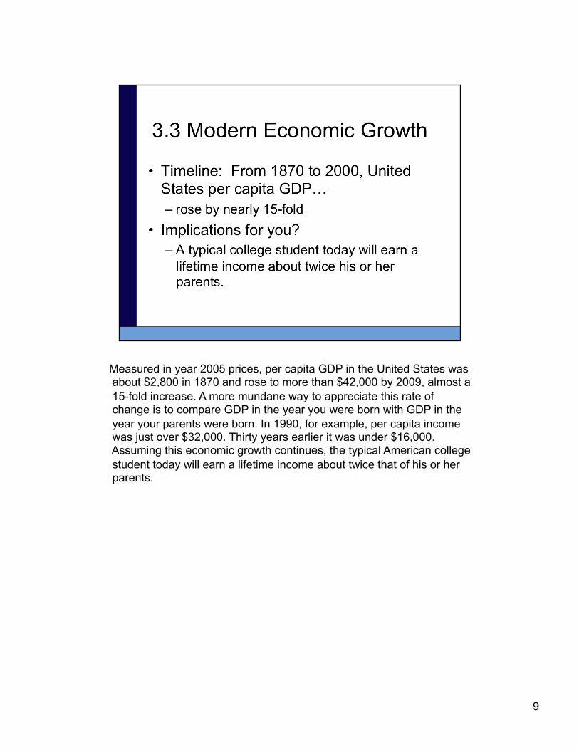
Teaching Tip: Click to label the variables one at a time

More generally, this example illustrates the following important result, known as the constant growth rule: if a variable starts at some initial value y0 at time 0 and grows at a constant rate g, then the value of the variable at some future time t is given as shown.

There is one more lesson to be learned from our simple population example. Equation (3.6) provides us with the size of the population at any time t, not just t = 100. In principle, we can use it to produce a plot of the population at each point in time.

14

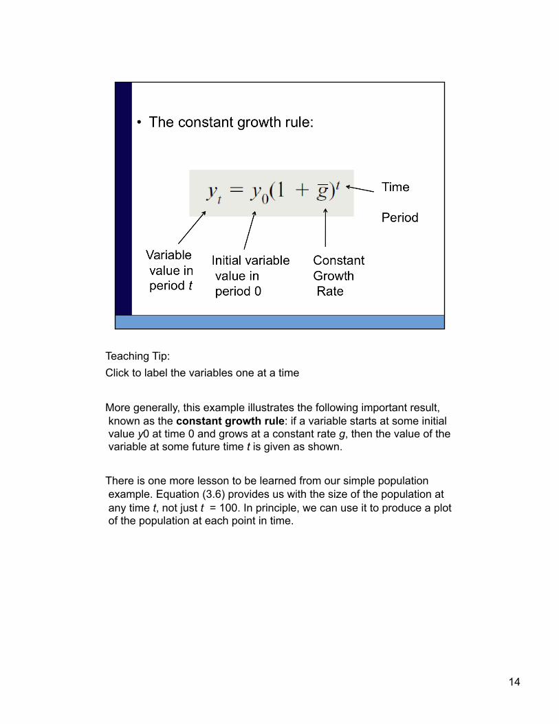
A major shortcoming of a figure like 3.2 or 3.3 is that it’s difficult to “see” the rate of growth in the figure. For example, is it possible to tell from Figure 3.3 that the rate of growth of the world population is constant over the 100 years? Not really. In Figure 3.2, is the average growth rate increasing, decreasing, or constant? Again, it’s nearly impossible to tell.

There are two points to note about the Rule of 70. First, it is very informative in its own right. If a country’s income grows at 1 percent per year, then it takes about 70 years for income to double. On the other hand, if growth is slightly faster at 5 percent per year, then income doubles every 14 (70/5) years. Seemingly small differences in growth rates lead to quite different outcomes when compounded over time. This is a point we will return to often throughout the next several chapters. The second implication of the Rule of 70 is that the time it takes for income to double depends only on the growth rate, not on the current level of income. If a country’s income grows at 2 percent per year, then it doubles every 35 years, regardless of whether the initial income is $500 or $25,000. How does this observation help us? First, let’s go back to our population example, reproduced in a slightly different way in Figure 3.4. In part (a), because population is growing at a constant rate of 2 percent per year, it will double every 35 years; the points when the population hits 6 billion (today), 12 billion, 24 billion, and 48 billion are highlighted.

15

16

Here is a graph of population over time. Once again, it is difficult to measure growth rates from year to year directly from this graph without doing some additional math and percentage changes. A ratio scale graph will help us more easily see growth rates.

In a ratio scale of 2, for example, indicates that each tick mark doubles from the previous.

On a normal graph with a standard scale, the slope of the graph will illustrate the absolute change. In a ratio scale graph, the slope of the graph will illustrate the rate of change.

Squishing the vertical axis this way creates a ratio scale: a plot where equally spaced tick marks on the vertical axis are labeled consecutively with numbers that exhibit a constant ratio, like “1, 2, 4, 8, . . .” (a constant ratio of 2) or “10, 100, 1,000, 10,000, . . .” (a constant ratio of 10). Plotted on a ratio scale, a variable growing at a constant rate appears as a straight line.

17

18

The left graph shows population increasing exponentially, but it is hard to see the growth rate. The right graphs shows a constant growth rate of population. Absolute population numbers are increasing faster, but the rate of growth is staying the same in the right graph because of the linear relationship.

The ratio scale for U.S. per capita GDP will be linear. The rate of growth is positive, but approximately constant.

The ratio scale is a tool that allows us to quickly read growth rates from a graph. For example, consider what we can learn by plotting U.S. per capita GDP on a ratio scale. If income grows at a constant rate, then the data points should lie on a straight line. Alternatively, if growth rates are rising, we would expect the slope between consecutive data points to be increasing.

19

The ratio scale for U.S. per capita GDP will be linear. The rate of growth is positive, but approximately constant.

The ratio scale is a tool that allows us to quickly read growth rates from a graph. For example, consider what we can learn by plotting U.S. per capita GDP on a ratio scale. If income grows at a constant rate, then the data points should lie on a straight line. Alternatively, if growth rates are rising, we would expect the slope between consecutive data points to be increasing.

20

21

Figure 3.5 shows the same data as Figure 3.2, per capita GDP in the United States, but now on a ratio scale. Notice that the vertical axis here is labeled “2, 4, 8, 16” — doubling over equally spaced intervals. Quite remarkably, the data series lies close to a line that exhibits a constant slope of 2.0 percent per year. This means that to a first approximation, per capita GDP in the United States has been growing at a relatively constant annual rate of 2.0 percent over the last 140 years. A closer look at the figure reveals that the growth rate in the first half of the sample was slightly lower than this. For example, the slope between 1870 and 1929 is slightly lower than that of the 2.0 percent line, while the slope between 1950 and 2009 is slightly higher. These are points that we can easily see on a ratio scale, as opposed to the standard linear scale in Figure 3.2.

If the data for every year are available, we could compute the percentage change across each annual period, and this would be a fine way to measure growth. But what if instead we are given data only for the start and end of this series?. We can use a growth rate equation. Teaching Tip: Emphasize the variables in the growth equation at the top already shown. Note that Yt is the dependent variable. To isolate the growth rate, we just need to solve for g. The rule for computing growth rates states that the average annual growth rate between periods 0 and t is equal to the ratio (yt/y0) raised to the 1/t power, all then minus 1. Note that if there were constant growth between year 0 and year t, the growth rate we compute would lead income to grow from y0 to yt. We can, however, apply this formula even to a data series that does not exhibit constant growth, like U.S. per capita GDP. In this case, we are calculating an average annual growth rate. In the special case where t = 1, this rule yields our familiar percentage change calculation for the growth rate, here (y1 - y0)/y0.

22

In the late nineteenth century, the United Kingdom was the richest country in the world, but it slipped from this position several decades later because it grew substantially slower than the United States. Notice how flat the per capita income line is for the U.K. relative to the United States. Since 1950, the United States and the U.K. have grown at more or less the same rate (indicated by the parallel lines), with income in the U.K. staying at about 3/4 the U.S. level. Germany and Japan are examples of countries whose incomes lagged substantially behind those of the United Kingdom and the United States over most of the last 135 years. Following World War II, however, growth in both countries accelerated sharply, with growth in Japan averaging nearly 6 percent per year between 1950 and 1990. The rapid growth gradually slowed in both, and incomes have stabilized at something like 3/4 the U.S. level for the last two decades, similar to the income level in the United Kingdom. This catch-up behavior is related to an important concept in the study of economic growth known as convergence.

23

24

When comparing levels of income on a ratio scale, recall that data points that are half below another country are actually much lower because the numbers on the vertical axis double. You might say that income levels in Germany and Japan have converged to the level in the United Kingdom during the postwar period. Economic growth in Brazil shows a different pattern, one that, to make a vast and somewhat unfair generalization, is more typical of growth in Latin America. Between 1900 and 1980, the country exhibited substantial economic growth, with income reaching nearly 1/3 the U.S. level. Since 1980, however, growth has slowed considerably, so that by 2006 income relative to the United States was just over 1/5. China shows something of the opposite pattern, with growth really picking up after 1978 and reaching rates of more than 7 percent per year for the last two decades. A country often grouped with China in such discussions is India, in part because the two countries together account for more than 40 percent of the world’s population. By 2006, China’s per capita income was about 1/5 the U.S. level, while India’s was just under 1/12. These last numbers may come as a surprise if you take only a casual glance at Figure 3.6; at first it appears that by 2006 China’s income was more than half the U.S. level. But remember that the graph is plotted on a ratio scale: look at the corresponding numbers on the vertical axis.

Growth rates between 1960 and 2007 range from 23% to 16% per year. Per capita GDP in 2007 varies by about a factor of 64 across countries.

25

26

The horizontal axis represents per capita GDP in the year 2007 relative to the United States. The vertical axis illustrates the wide range of growth rates that countries have experienced since 1960. Hong Kong, Norway, Singapore, and the United States had the highest per capita GDP in the world that year. Other rich countries include Ireland, Israel, Japan, South Korea, and Spain, with incomes greater than 1/2 the U.S. level. Middle-income countries like Honduras, Mexico, and Argentina had incomes about 1/3 the U.S. level. China, India, and Indonesia are examples of countries with relative incomes between 1/16 and 1/5. Finally, Burundi, Niger, and Tanzania, among the poorest countries of the world in 2007, had incomes as low as 1/64 the U.S. level. The fastest-growing countries over this period include South Korea, Hong Kong, Thailand, China, Botswana, and Japan, all with average growth rates between 4 and 6 percent per year. At the other end of the spectrum are the Central African Republic, the Democratic Republic of the Congo, Niger, and Zimbabwe, each of which exhibited negative average growth over this half century. The bulk of the countries lie between these two extremes. In Taiwan, for example, which is growing at 6 percent per year, incomes will double every 12 years (remember the Rule of 70).

27

28

The graph shows, for 1960 and 2007, the percentage of the world’s population living in countries with a per capita GDP less than or equal to the number on the horizontal axis. This per capita GDP is relative to the United States in the year 2007 for both lines.

China and India are highlighted.

Teaching Tip: Note that ratio = division, product = multiplication, and powers = exponents (squared, cubed, etc).

29

Teaching Tip: The best way to explain these rules is to just look at the examples on the next slides. There are two tables, both showing the same examples, but one table is zoomed in to see the numbers better.

30

31

Regular-sized table 3.1.

32

Zoomed in table 3.1.

Teaching Tip: Go through the math here step-by-step, perhaps even filling in the given values for gx, gy, and solving for gz. It would be a good in-class exercise.

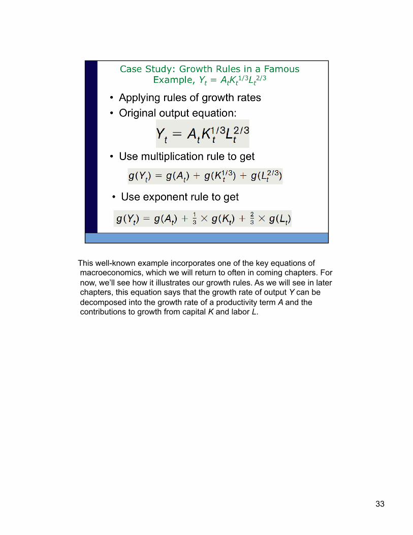
This well-known example incorporates one of the key equations of macroeconomics, which we will return to often in coming chapters. For now, we’ll see how it illustrates our growth rules. As we will see in later chapters, this equation says that the growth rate of output Y can be decomposed into the growth rate of a productivity term A and the contributions to growth from capital K and labor L.

33

34

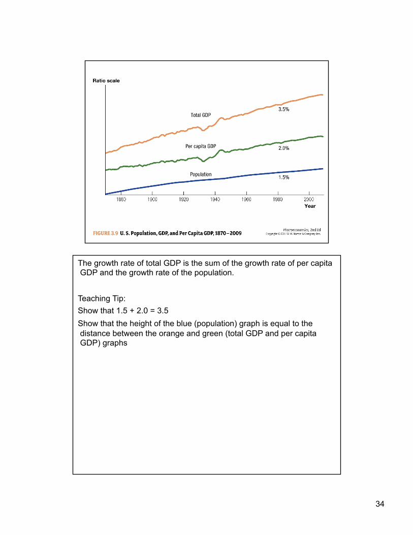
The growth rate of total GDP is the sum of the growth rate of per capita GDP and the growth rate of the population.

Teaching Tip: Show that 1.5 + 2.0 = 3.5 Show that the height of the blue (population) graph is equal to the distance between the orange and green (total GDP and per capita GDP) graphs

Teaching Tip: Remind the students that in economics, it can often come down to analyzing marginal benefit vs marginal cost.

When we consider economic growth, what usually comes to mind are the enormous benefits it brings: increases in life expectancy, reductions in infant mortality, higher incomes, an expansion in the range of goods and services available, and so on. But what about the costs of economic growth? High on the list of costs are environmental problems such as pollution, the depletion of natural resources, and even global warming. Another by-product of economic growth during the last century is increased income inequality — certainly across countries and perhaps even within countries. Technological advances may also lead to the loss of certain jobs and industries. For example, automobiles decimated the horse-and-buggy industry; telephone operators and secretaries have seen their jobs redefined as information technology improves. More than 40 percent of U.S. workers were employed in agriculture in 1900; today the fraction is less than 2 percent. The general consensus among economists who have studied these costs is that they are substantially outweighed by the overall benefits. In the poorest regions of the world, this is clear. When 20 percent of children die before the age of 5 — as they do in much of Africa — the essential problem is not pollution or too much technological progress, but rather the absence of economic growth. But the benefits also outweigh the costs in richer countries. For example, while pollution is often associated with the early stages of economic growth — as in London in the mid-1800s or Mexico City today — environmental economists have documented an inverse-U shape for this relationship. Pollution grows worse initially as an economy develops, but it often gets better eventually. Smog levels in Los Angeles are substantially less today than they were 30 years ago; one reason may be that cars in California produce noxious emissions that are only 5 percent of their levels in the mid-1970s. Technological change undoubtedly eliminates some jobs, and there is no denying the hardship that this can cause in the short run.

35

36

This slide is a preview of what will be studied in the next chapters.

37

38

39

40

41

42

43

These are some tables and graphs that appear in the practice problems at the end of the chapter. Some instructors may want to show them during class for examples.

44

45

46

47