10/19/2011

1

Solving Systems of Equations

“Numerical Methods with MATLAB”, Recktenwald, Chapter 8and

“Numerical Methods for Engineers”, Chapra and Canale, 5th Ed., Part Three, Chapters 9 to 11 and

“Applied Numerical Methods with MATLAB”, Chapra, 2nd Ed., Part Three, Chapters 8 to 12

PGE 310: Formulation and Solution in Geosystems Engineering

Dr. Balhoff

1

Solving Systems of Equations

Many Science & Engineering problems require the solution to systems of equations

General Rule: Need as many (unique) equations as unknowns

Guide to putting equations in Natural Form:1. Write the equations in their natural form

2. Identify Unknowns, and order them

3. Isolate the unknowns

4. Write Equations in Matrix form (Ax=b)

11 1 12 2 1 1

21 1 22 2 2 2

1 1 2 2

n n

n n

n n nn n n

a x a x a x b

a x a x a x b

a x a x a x b

Ax b

2

10/19/2011

2

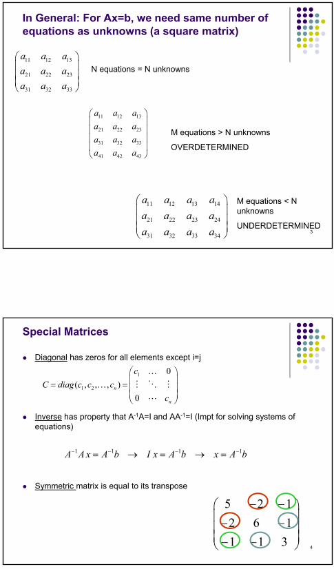
In General: For Ax=b, we need same number of equations as unknowns (a square matrix)

11 12 13

21 22 23

31 32 33

a a a

a a a

a a a

11 12 13

21 22 23

31 32 33

41 42 43

a a a

a a a

a a a

a a a

11 12 13 14

21 22 23 24

31 32 33 34

a a a a

a a a a

a a a a

N equations = N unknowns

M equations > N unknowns

OVERDETERMINED

M equations < N unknowns

UNDERDETERMINED3

Special Matrices

Diagonal has zeros for all elements except i=j

Inverse has property that A-1A=I and AA-1=I (Impt for solving systems of equations)

Symmetric matrix is equal to its transpose

1

1 2

0

( , , , )

0n

n

c

C diag c c c

c

5 2 1

2 6 1

1 1 3

4

bAxbAxIbAxAA 1111

10/19/2011

3

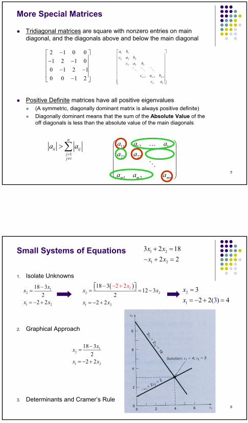
More Special Matrices

Tridiagonal matrices are square with nonzero entries on main diagonal, and the diagonals above and below the main diagonal

Positive Definite matrices have all positive eigenvalues (A symmetric, diagonally dominant matrix is always positive definite)

Diagonally dominant means that the sum of the Absolute Value of the off diagonals is less than the absolute value of the main diagonals

1

n

ii ijjj i

a a

11 12 1

21 22

1 2

n

m m mn

a a a

a a

a a a

2 1 0 0

1 2 1 0

0 1 2 1

0 0 1 2

1 1

2 2 2

3 3 3

1 1 1n n n

n n

a b

c a b

c a b

c a b

c a

5

Small Systems of Equations

1. Isolate Unknowns

2. Graphical Approach

3. Determinants and Cramer’s Rule

1 2

1 2

3 2 18

2 2

x x

x x

12

1 2

18 3

22 2

xx

x x

2 2

1

2

2

18 312 3

2

2

2 2

2x x

x

x x

2

1

3

2 2( ) 43

x

x

12

1 2

18 3

22 2

xx

x x

6

10/19/2011

4

Requirements for a solution

Need as many (unique) equations as unknowns

Having a square matrix (n equations and n unknowns) isn’t good enough

The matrix A must be non-singular, or the rank(A) must equal n The rows must be linearly independent

7

Gauss Elimination is a Fundamental procedure for solving systems of linear equations

Diagonal systems are easy:

Consider the following:

1 0 0 1

0 3 0 , 6

0 0 5 15

A b

1

2

3

1

3 6

5 15

x

x

x

x3 = -15/5 = -3

x2 = 6/3 = 2

x1 = -1/1 = -1

Back Substitution

8

10/19/2011

5

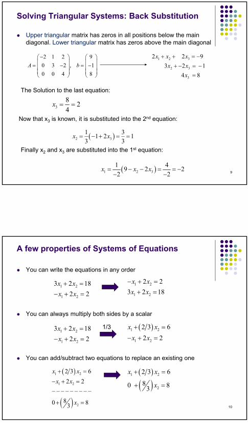
Solving Triangular Systems: Back Substitution

Upper triangular matrix has zeros in all positions below the main diagonal. Lower triangular matrix has zeros above the main diagonal

2 1 2 9

0 3 2 , 1

0 0 4 8

A b

1 2 3

2 3

3

2 2 9

3 2 1

4 8

x x x

x x

x

3

82

4x

2 3

1 31 2 1

3 3x x

1 2 3

1 49 2 2

2 2x x x

The Solution to the last equation:

Now that x3 is known, it is substituted into the 2nd equation:

Finally x2 and x3 are substituted into the 1st equation:

9

A few properties of Systems of Equations

You can write the equations in any order

You can always multiply both sides by a scalar

You can add/subtract two equations to replace an existing one

1 2

1 2

2 2

3 2 18

x x

x x

1 2

1 2

3 2 18

2 2

x x

x x

1 2

1 2

2 3 6

2 2

x x

x x

1 2

1 2

3 2 18

2 2

x x

x x

1/3

1 2

1 2

2

2 3 6

2 2

80 83

x x

x x

x

1 2

2

2 3 6

80 83

x x

x

10

10/19/2011

6

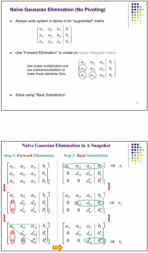
Naïve Gaussian Elimination (No Pivoting)

Always write system in terms of an “augmented” matrix

Use “Forward Elimination” to create an upper triangular matrix

Solve using “Back Substitution”

11 12 13 1

21 22 23 2

31 32 33 3

a a a b

a a a b

a a a b

11 12 13 1

21 22 23 2

31 32 33 3

a a a b

a a a b

a a a b

Use scalar multiplication and row subtraction/addition to make these elements Zero

11

333

22322

1131211

00

0

ba

baa

baaa

Naïve Gaussian Elimination in A Snapshot

Step 1: Forward Elimination

3333231

2232221

1131211

baaa

baaa

baaa

33332

22322

1131211

0

0

baa

baa

baaa

333

22322

1131211

00

0

ba

baa

baaa

Step 2: Back Substitution

333

22322

1131211

00

0

ba

baa

baaa

3x

2x

1x

333

22322

1131211

00

0

ba

baa

baaa

10/19/2011

7

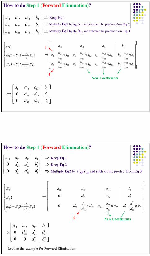
How to do Step 1 (Forward Elimination)?

3333231

2232221

1131211

baaa

baaa

baaa Keep Eq 1

Multiply Eq1 by a21/a11 and subtract the product from Eq 2

Multiply Eq1 by a31/a11 and subtract the product from Eq 3

133

122

1

11

31

11

21

Eqa

aEqEq

Eqa

aEqEq

Eq

111

31313

11

313312

11

313211

11

3131

111

21213

11

212312

11

212211

11

2121

1131211

ba

aba

a

aaa

a

aaa

a

aa

ba

aba

a

aaa

a

aaa

a

aa

baaa

0

0

New Coefficients

33332

22322

1131211

0

0

baa

baa

baaa

How to do Step 1 (Forward Elimination)?

233

2

1

22

32 Eqa

aEqEq

Eq

Eq

222

32323

22

323322

22

3232

22322

1131211

0

0

ba

aba

a

aaa

a

aa

baa

baaa

0 New Coefficients

33332

22322

1131211

0

0

baa

baa

baaa Keep Eq 1

Keep Eq 2

Multiply Eq2 by a’32/a’22 and subtract the product from Eq 3

333

22322

1131211

00

0

ba

baa

baaa

Look at the example for Forward Elimination

10/19/2011

8

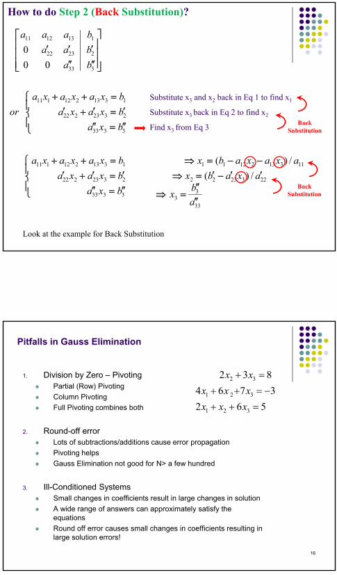
How to do Step 2 (Back Substitution)?

Substitute x3 and x2 back in Eq 1 to find x1

Substitute x3 back in Eq 2 to find x2

Find x3 from Eq 3

Look at the example for Back Substitution

333

22322

1131211

00

0

ba

baa

baaa

3333

2323222

1313212111

bxa

bxaxa

bxaxaxa

or

33

33

2232322

1131321211

3333

2323222

1313212111

/)(

/)(

a

bx

axabx

axaxabx

bxa

bxaxa

bxaxaxa

Back Substitution

Back Substitution

Pitfalls in Gauss Elimination

1. Division by Zero – Pivoting Partial (Row) Pivoting

Column Pivoting

Full Pivoting combines both

2. Round-off error Lots of subtractions/additions cause error propagation

Pivoting helps

Gauss Elimination not good for N> a few hundred

3. Ill-Conditioned Systems Small changes in coefficients result in large changes in solution

A wide range of answers can approximately satisfy the equations

Round off error causes small changes in coefficients resulting in large solution errors!

2 3

1 2 3

1 2 3

2 3 8

4 6 7 3

2 6 5

x x

x x x

x x x

16

10/19/2011

9

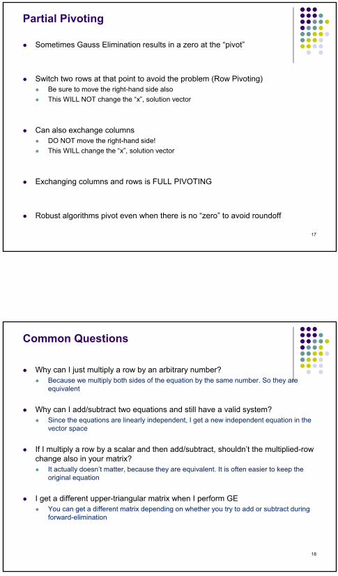
Partial Pivoting

Sometimes Gauss Elimination results in a zero at the “pivot”

Switch two rows at that point to avoid the problem (Row Pivoting) Be sure to move the right-hand side also

This WILL NOT change the “x”, solution vector

Can also exchange columns DO NOT move the right-hand side!

This WILL change the “x”, solution vector

Exchanging columns and rows is FULL PIVOTING

Robust algorithms pivot even when there is no “zero” to avoid roundoff

17

Common Questions

Why can I just multiply a row by an arbitrary number? Because we multiply both sides of the equation by the same number. So they are

equivalent

Why can I add/subtract two equations and still have a valid system? Since the equations are linearly independent, I get a new independent equation in the

vector space

If I multiply a row by a scalar and then add/subtract, shouldn’t the multiplied-row change also in your matrix? It actually doesn’t matter, because they are equivalent. It is often easier to keep the

original equation

I get a different upper-triangular matrix when I perform GE You can get a different matrix depending on whether you try to add or subtract during

forward-elimination

18

10/19/2011

10

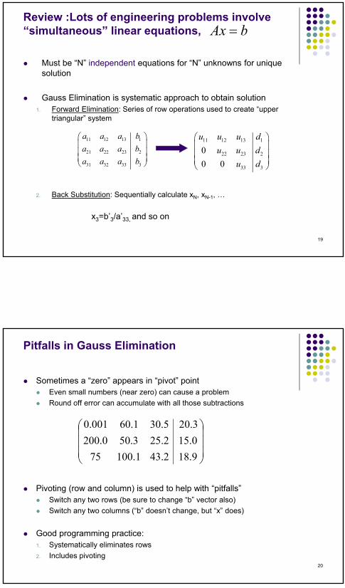
Review :Lots of engineering problems involve “simultaneous” linear equations,

Must be “N” independent equations for “N” unknowns for unique solution

Gauss Elimination is systematic approach to obtain solution1. Forward Elimination: Series of row operations used to create “upper

triangular” system

2. Back Substitution: Sequentially calculate xN, xN-1, …

bAx

11 12 13 1

21 22 23 2

31 32 33 3

a a a b

a a a b

a a a b

11 12 13 1

22 23 2

33 3

0

0 0

u u u d

u u d

u d

x3=b’3/a’33, and so on

19

Pitfalls in Gauss Elimination

Sometimes a “zero” appears in “pivot” point Even small numbers (near zero) can cause a problem

Round off error can accumulate with all those subtractions

Pivoting (row and column) is used to help with “pitfalls” Switch any two rows (be sure to change “b” vector also)

Switch any two columns (“b” doesn’t change, but “x” does)

Good programming practice: 1. Systematically eliminates rows

2. Includes pivoting

9.182.431.10075

0.152.253.500.200

3.205.301.60001.0

20

10/19/2011

11

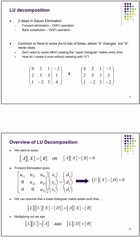
LU decomposition

2 steps in Gauss Elimination 1. Forward elimination – O(N3) operation

2. Back substitution – O(N2) operation

Common to have to solve Ax=b lots of times, where “b” changes but “A” never does

Don’t want to waste effort creating the “upper triangular” matrix every time

How do I create it once without messing with “b”?

4321

1352

2124

2321

3352

1124&

21

Overview of LU Decomposition

We want to solve

Forward Elimination gives

We can assume that a lower-triangular matrix exists such that….

Multiplying out we see

A X B 0A X B

0U X D

L U X D A X B

L U A L D B

11 21 31 1 1

22 23 2 2

33 3 3

0

0 0

u u u x d

u u x d

u x d

OR

AND22

10/19/2011

12

Overview of LU Decomposition

23

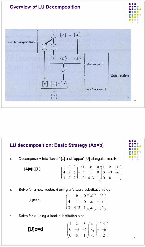
LU decomposition: Basic Strategy (Ax=b)

1. Decompose A into “lower” [L] and “upper” [U] triangular matrix:

[A]=[L][U]

1. Solve for a new vector, d using a forward substitution step:

[L]d=b

2. Solve for x, using a back substitution step:

[U]x=d

1 2 3 1 0 0 1 2 3

4 5 6 4 1 0 0 3 6

3 2 2 3 4 / 3 1 0 0 1

1

2

3

1 0 0 3

4 1 0 6

3 4 / 3 1 3

d

d

d

1

2

3

1 2 3 3

0 3 6 6

0 0 1 2

x

x

x

24

10/19/2011

13

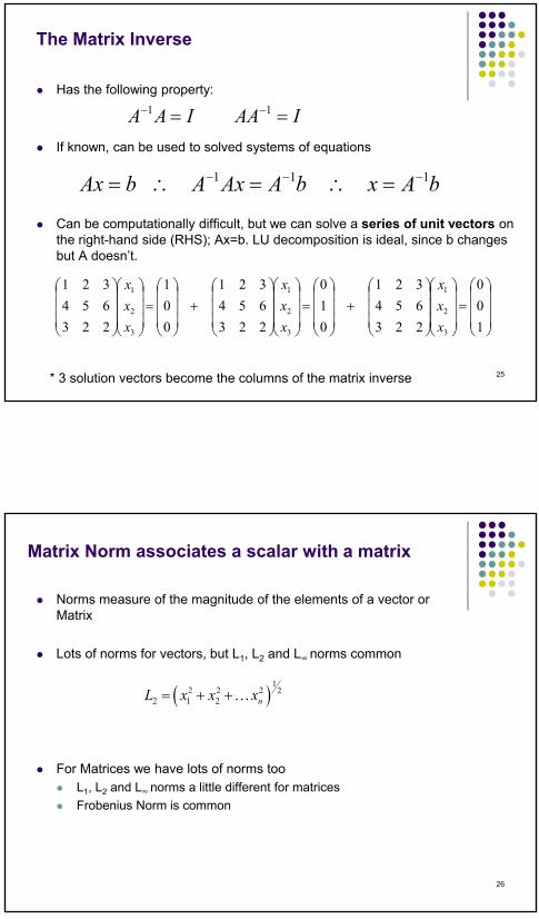
The Matrix Inverse

Has the following property:

If known, can be used to solved systems of equations

Can be computationally difficult, but we can solve a series of unit vectors on the right-hand side (RHS); Ax=b. LU decomposition is ideal, since b changes but A doesn’t.

IAAIAA 11

bAxbAAxAbAx 111

1

0

0

223

654

321

0

1

0

223

654

321

0

0

1

223

654

321

3

2

1

3

2

1

3

2

1

x

x

x

x

x

x

x

x

x

* 3 solution vectors become the columns of the matrix inverse 25

Matrix Norm associates a scalar with a matrix

Norms measure of the magnitude of the elements of a vector or Matrix

Lots of norms for vectors, but L1, L2 and L∞ norms common

For Matrices we have lots of norms too L1, L2 and L∞ norms a little different for matrices

Frobenius Norm is common

1

2 2 2 22 1 2 nL x x x

26

10/19/2011

14

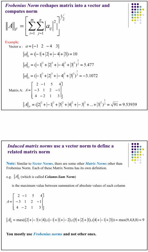
Frobenius Norm reshapes matrix into a vector and computes norm

12

2

1 1

m n

ijFi j

A a

Example: Vector a :

Matrix A:

]3421[ a

1072.3)3421(

477.5)3421(

10)3421(

3

13333

3

2

12222

2

1

a

a

a

3124

1213

4512

A

53939.991)3...34512( 2

1222222

FA

Induced matrix norms use a vector norm to define a related matrix norm

Note: Similar to Vector Norms, there are some other Matrix Norms other than Frobenius Norm. Each of these Matrix Norms has its own definition.

e.g. (which is called Column-Sum Norm)

is the maximum value between summation of absolute values of each column

1A

9)8,8,4,9max())314(),125(),211(),432max((

3124

1213

4512

1

A

A

You mostly use Frobenius norms and not other ones.

10/19/2011

15

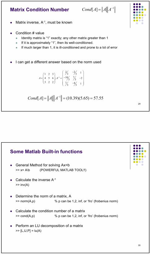
Matrix Condition Number

Matrix inverse, A-1, must be known

Condition # value Identity matrix is “1” exactly; any other matrix greater than 1

If it is approximately “1”, then its well-conditioned.

If much larger than 1, it is ill-conditioned and prone to a lot of error

I can get a different answer based on the norm used

1][ AAACond

1

2 2 13 31 2 310 74 5 6 ; 23 3

3 2 2 7 4 13 3

A A

1[ ] (10.39)(5.65) 57.55Cond A A A 29

Some Matlab Built-in functions

General Method for solving Ax=b>> x= A\b (POWERFUL MATLAB TOOL!!)

Calculate the inverse A-1

>> inv(A)

Determine the norm of a matrix, A>> norm(A,p) % p can be 1,2, inf, or ‘fro’ (frobenius norm)

Calculate the condition number of a matrix>> cond(A,p) % p can be 1,2, inf, or ‘fro’ (frobenius norm)

Perform an LU decomposition of a matrix>> [L,U,P] = lu(A)

30

10/19/2011

16

Direct Methods for solving systems of equations

Gauss Elimination and LU decomposition are direct (elimination) methods Forward elimination to get upper triangular matrix

Substitution to solve for x-vector

Some pitfalls and drawbacks to direct methods Slow for systems larger than a few hundred (elimination is an O(N3) process)

Roundoff error can propagate for large equations even with pivoting

Need an alternative for large equations (>1000)

31

Indirect (Iterative) Methods offer alternative to elimination

Idea: Guess a vector x(0) and systematically refine the root

Sort of like fixed-point iteration Write each of the “N” equations explicitly in terms of x1,x2, etc.

Solve for each new xi using old guess values

3 Iterative methods (that are quite similar) Jacobi

Gauss-Seidel

Successive (Over)-Relaxation (SOR)

32

10/19/2011

17

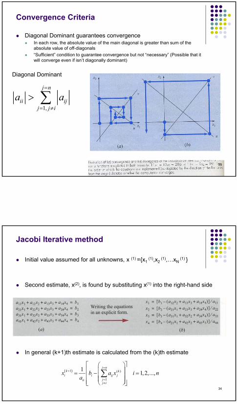
Convergence Criteria

Diagonal Dominant guarantees convergence In each row, the absolute value of the main diagonal is greater than sum of the

absolute value of off-diagonals

“Sufficient” condition to guarantee convergence but not “necessary” (Possible that it will converge even if isn’t diagonally dominant)

1,

j n

ii ijj j i

a a

Diagonal Dominant

33

Jacobi Iterative method

Initial value assumed for all unknowns, x (1) ={x1 (1),x2

(1),…xN (1) }

Second estimate, x(2), is found by substituting x(1) into the right-hand side

In general (k+1)th estimate is calculated from the (k)th estimate

1 ( )

1

11,2,...,

j nk ki i ij j

jiij i

x b a x i na

34

10/19/2011

18

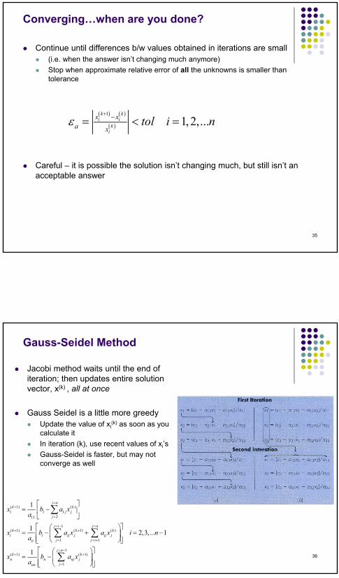
Converging…when are you done?

Continue until differences b/w values obtained in iterations are small (i.e. when the answer isn’t changing much anymore)

Stop when approximate relative error of all the unknowns is smaller than tolerance

Careful – it is possible the solution isn’t changing much, but still isn’t an acceptable answer

1

1, 2,...k ki i

ki

x xa x

tol i n

35

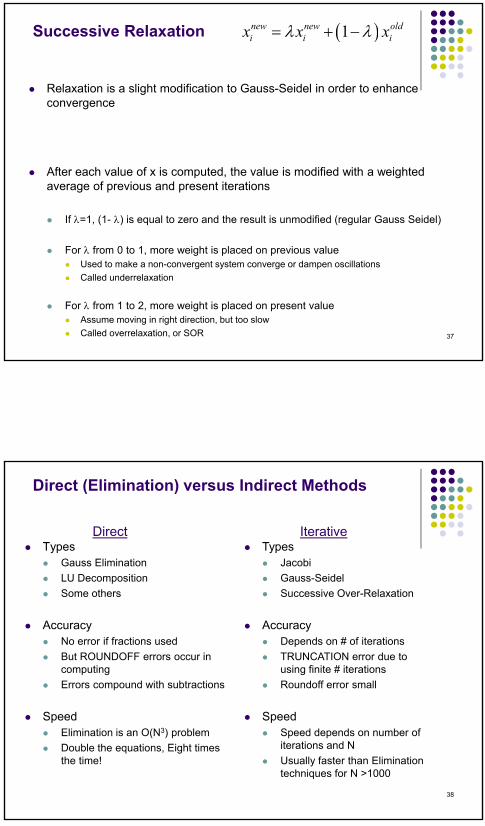
Gauss-Seidel Method

Jacobi method waits until the end of iteration; then updates entire solution vector, x(k) , all at once

Gauss Seidel is a little more greedy Update the value of xi

(k) as soon as you calculate it

In iteration (k), use recent values of xi’s

Gauss-Seidel is faster, but may not converge as well

( 1) ( )1 1 1

211

1( 1) ( 1) ( )

1 1

1( 1) ( 1)

1

1

12,3,... 1

1

j nk k

j jj

j i j nk k ki i ij j ij j

j j iii

j nk kn n nj j

jnn

x b a xa

x b a x a x i na

x b a xa

36

10/19/2011

19

Successive Relaxation

Relaxation is a slight modification to Gauss-Seidel in order to enhance convergence

After each value of x is computed, the value is modified with a weighted average of previous and present iterations

If =1, (1- ) is equal to zero and the result is unmodified (regular Gauss Seidel)

For from 0 to 1, more weight is placed on previous value Used to make a non-convergent system converge or dampen oscillations

Called underrelaxation

For from 1 to 2, more weight is placed on present value Assume moving in right direction, but too slow

Called overrelaxation, or SOR

1new new oldi i ix x x

37

Direct (Elimination) versus Indirect Methods

Types Gauss Elimination

LU Decomposition

Some others

Accuracy No error if fractions used

But ROUNDOFF errors occur in computing

Errors compound with subtractions

Speed Elimination is an O(N3) problem

Double the equations, Eight times the time!

Types Jacobi

Gauss-Seidel

Successive Over-Relaxation

Accuracy Depends on # of iterations

TRUNCATION error due to using finite # iterations

Roundoff error small

Speed Speed depends on number of

iterations and N

Usually faster than Elimination techniques for N >1000

Direct Iterative

38

10/19/2011

20

Review… Systems of Linear Equations

Common in Science and Engineering (and college football!)

Direct Methods – error dominated by roundoff Gauss Elimination

LU decomposition

Iterative Methods – error dominated by truncation Jacobi

Gauss Seidel (w/ or w/o relaxation)

39

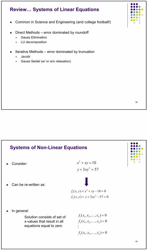
Systems of Non-Linear Equations

Consider:

Can be re-written as:

In general:

2

2

10

3 57

x xy

y xy

21

22

( , ) 10 0

( , ) 3 57 0

f x y x xy

f x y y xy

1 1 2

2 1 2

1 2

( , , , ) 0

( , , , ) 0

( , , , ) 0

n

n

n n

f x x x

f x x x

f x x x

Solution consists of set of x-values that result in all equations equal to zero

40

10/19/2011

21

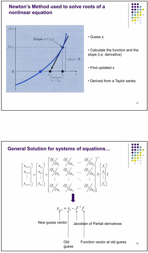
Newton’s Method used to solve roots of a nonlinear equation

• Guess x

• Calculate the function and the slope (i.e. derivative)

• Find updated x

• Derived from a Taylor series

41

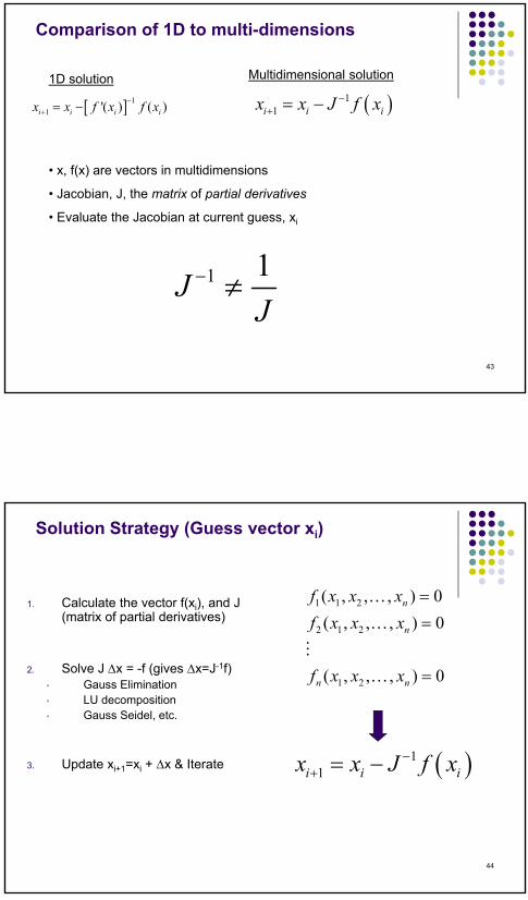
General Solution for systems of equations…

1

1 1 1

1 21, 1 1, 1

2 2 22, 1 2, 2

1 2

, 1 ,

1 2

ni i

i in

n i n i nn n n

n

f f fx x xx x f

f f fx x fx x x

x x ff f fx x x

11i ix x J f

New guess vector

Old guess

Jacobian of Partial derivatives

Function vector at old guess 42

(- )

10/19/2011

22

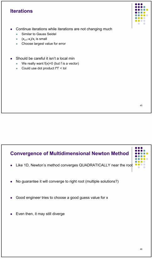
Comparison of 1D to multi-dimensions

11i i ix x J f x 1

1 '( ) ( )i i i ix x f x f x

1D solution Multidimensional solution

• x, f(x) are vectors in multidimensions

• Jacobian, J, the matrix of partial derivatives

• Evaluate the Jacobian at current guess, xi

1 1J

J

43

Solution Strategy (Guess vector xi)

1. Calculate the vector f(xi), and J (matrix of partial derivatives)

2. Solve J x = -f (gives x=J-1f)• Gauss Elimination• LU decomposition• Gauss Seidel, etc.

3. Update xi+1=xi + x & Iterate 11i i ix x J f x

1 1 2

2 1 2

1 2

( , , , ) 0

( , , , ) 0

( , , , ) 0

n

n

n n

f x x x

f x x x

f x x x

44

10/19/2011

23

Iterations

Continue iterations while iterations are not changing much Similar to Gauss Seidel

(xi+1-xi)/xi is small

Choose largest value for error

Should be careful it isn’t a local min We really want f(x)=0 (but f is a vector)

Could use dot product f*f’ < tol

45

Convergence of Multidimensional Newton Method

Like 1D, Newton’s method converges QUADRATICALLY near the root

No guarantee it will converge to right root (multiple solutions?)

Good engineer tries to choose a good guess value for x

Even then, it may still diverge

46