CH2. The Principles of Eddy Current Testing 2.1. Introduction

The eddy current testing method is a form of electromagnetic nondestructive testing based on the principles of electromagnetic induction. The physicals of eddy current testing are shown in figure 2.1. The Maxwell-Ampere law states that an alternating current sets up a time varying magnetic field. When a primary coil excited with an alternating current is placed in close proximity to a conducting surface, the alternating primary magnetic fields from the probe interact with the law. This induced voltage produces eddy currents in the material witch, by Lenz's Law (楞次定律), set up secondary magnetic fields that oppose the ones producing them. The eddy currents, thus, are analogous to a mutually coupled secondary circuit in witch the current flows in a circular direction opposite that of the current in the coil. This mutual inductance causes a change in the impedance of the coil because the load of the secondary circuit, now the eddy currents in the specimen, are referred, or "reflected", back to the primary coil. For instance, the resistive component is a measure of the energy losses within the material since the eddy currents represent a resistive load. Hence, as a coil is brought close to a non-ferromagnetic conductive material (非鐵磁性材料) its resistance, the real component of its impedance, increases.

1

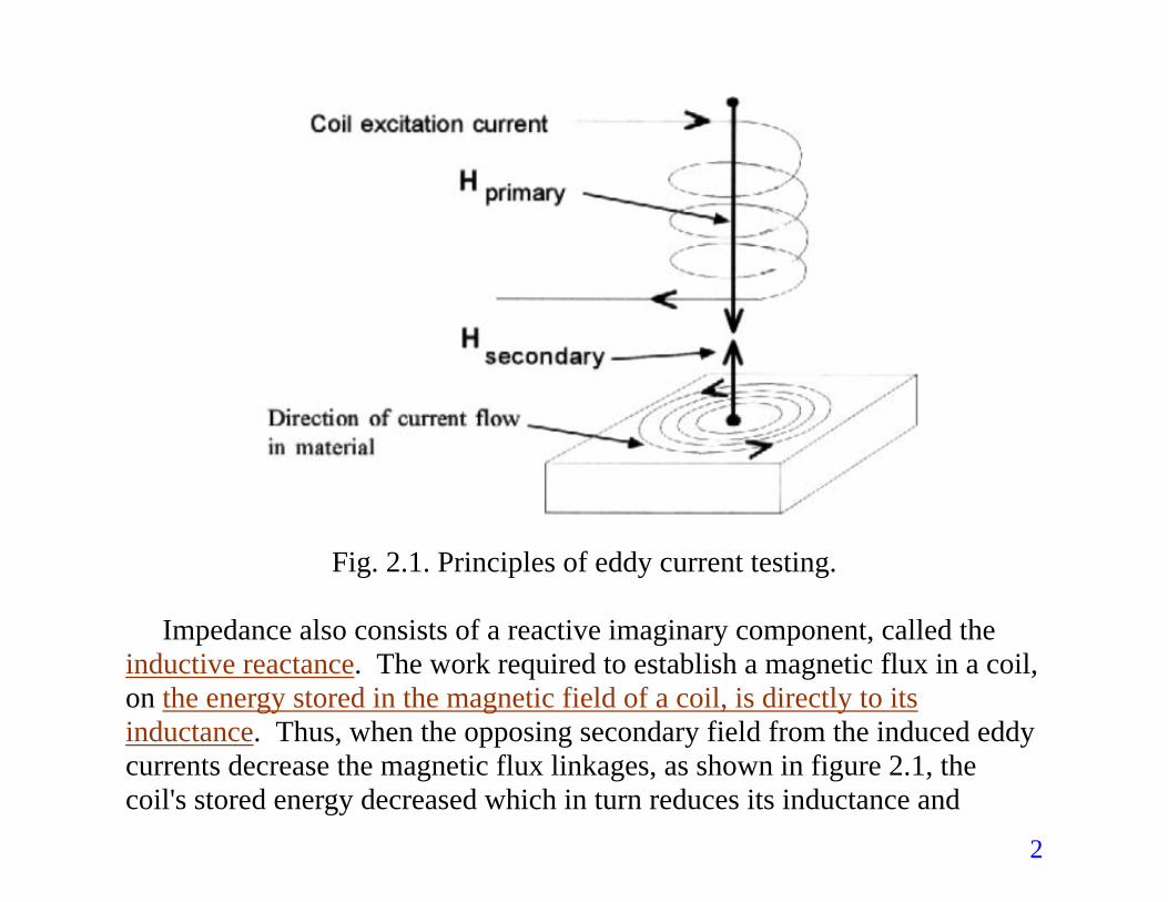
Fig. 2.1. Principles of eddy current testing.

Impedance also consists of a reactive imaginary component, called the

inductive reactance. The work required to establish a magnetic flux in a coil, on the energy stored in the magnetic field of a coil, is directly to its inductance. Thus, when the opposing secondary field from the induced eddy currents decrease the magnetic flux linkages, as shown in figure 2.1, the coil's stored energy decreased which in turn reduces its inductance and 2

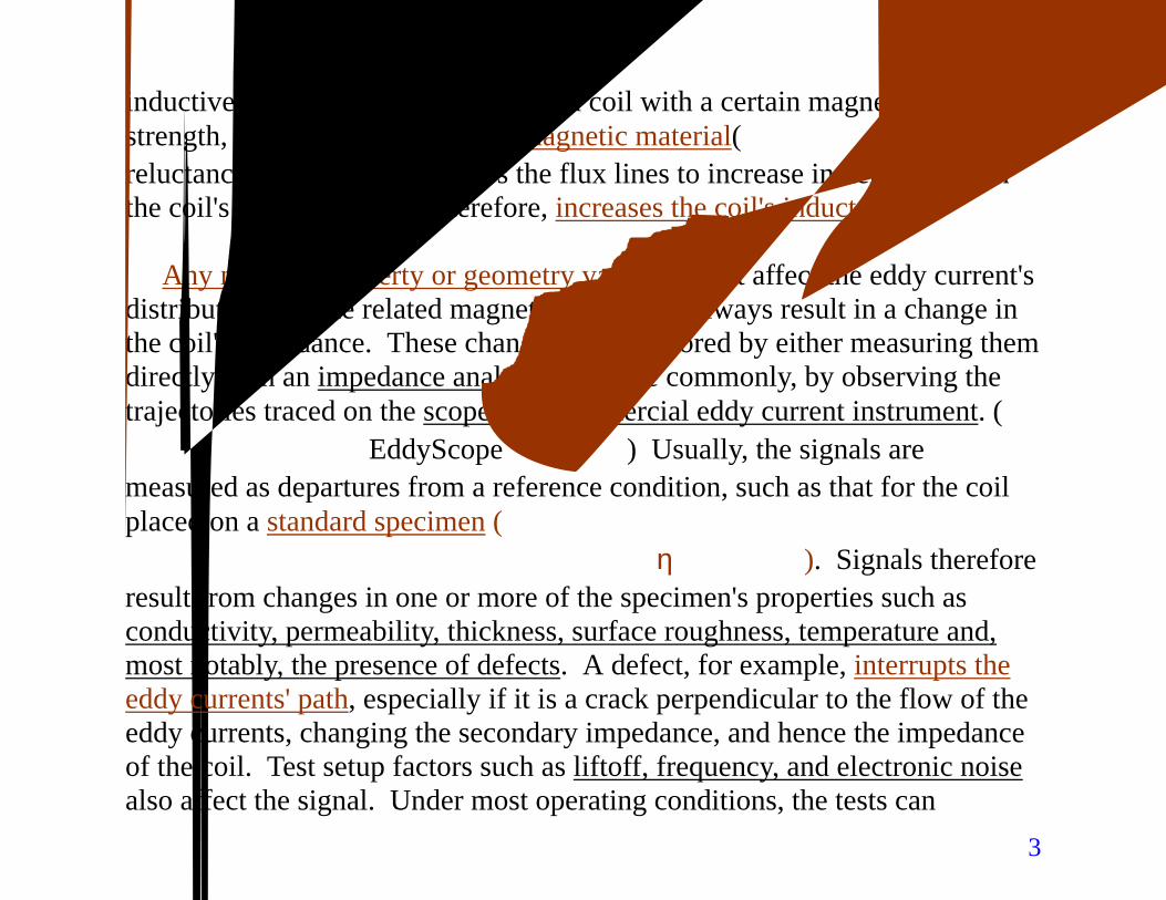
inductive reactance. However, when a coil with a certain magnetic field strength, H, is placed over a ferromagnetic material(鐵磁性材料), the lower reluctance in the material allows the flux lines to increase in density within the coil's windings. This, therefore, increases the coil's inductance.

Any material property or geometry variances that affect the eddy current's distribution and the related magnetic fields will always result in a change in the coil's impedance. These changes are monitored by either measuring them directly with an impedance analyzer or, more commonly, by observing the trajectories traced on the scope of a commercial eddy current instrument. (一般以阻抗分析儀或 EddyScope觀察紀錄) Usually, the signals are measured as departures from a reference condition, such as that for the coil placed on a standard specimen (若無理論值可驗證，則需有標準樣本作為比對，一般工場採用此法，可以想見需有多少樣本！). Signals therefore result from changes in one or more of the specimen's properties such as conductivity, permeability, thickness, surface roughness, temperature and, most notably, the presence of defects. A defect, for example, interrupts the eddy currents' path, especially if it is a crack perpendicular to the flow of the eddy currents, changing the secondary impedance, and hence the impedance of the coil. Test setup factors such as liftoff, frequency, and electronic noise also affect the signal. Under most operating conditions, the tests can 3

differentiate between various factors and material properties if they each produce a different signal response. For example, commercial eddy scopes will display relatively distinctive trajectories for different types of deviations. This allows the instrument to be setup in a way that separates an unwanted signal, such as that caused from liftoff, from the signal of interest, such as a flaw. Recorded signals can also be processed later by removing the noisy responses known to be caused by certain factors.

Commercial eddy current instruments are almost exclusively used in a

relative nature where reference standards are used to set the normal operating point. A material similar to the standard is tested by observing the signals that deviate from the reference condition; these indicate flaws or other property changes. A good understanding of these signals and how an instrument detects and displays them is necessary to develop a simple calibration method that would make quantitative impedance measurements possible. Consequently, commercial instruments would be able to perform quantitative NDE (QNDE), such as is now performed with an impedance analyzer in conjunction with an applicable eddy current theory.

4

2.2. Theory of Eddy Current Phenomenon

Electromagnetic phenomenon for time varying conditions are governed by Maxwell's equations as follows:

tBE

∂∂

−=×∇ (2.1)

∂

tDJH

∂+=×∇ (2.2)

0=⋅∇ B (2.3)

ρ=⋅∇ D (2.4)

The constitutive relations for an isotropic, linear and homogeneous

medium are given as HB µ= (2.5) ED ε= (2.6) EJ σ= (2.7)

where

5

µ = the magnetic permeability in henrys per meter(H/m) ε = the electric permittivity in farads per meter (F/m), and σ = the electric conductivity in seimens per meter (S/m).

Since the divergence of B is zero from equation (2.3), B can be expressed as the curl of another vector, called the magnetic vector potential (MVP) A, given by

.AB ×∇= (2.8) Combining this with equation (2.1) gives

tAE

∂∂

×−∇=×∇ (2.9)

or

0=

∂∂

+×∇tAE (2.10)

Since an irrotational field can be replaced with the gradient of a scalar

6

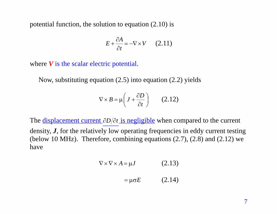
potential function, the solution to equation (2.10) is

VtAE ×−∇=

∂∂

+ (2.11)

where V is the scalar electric potential.

Now, substituting equation (2.5) into equation (2.2) yields

∂∂

+=×∇tDJB µ (2.12)

The displacement current tD ∂∂ is negligible when compared to the current density, J, for the relatively low operating frequencies in eddy current testing (below 10 MHz). Therefore, combining equations (2.7), (2.8) and (2.12) we have

JA µ=×∇×∇ (2.13)

Eµσ= (2.14) 7

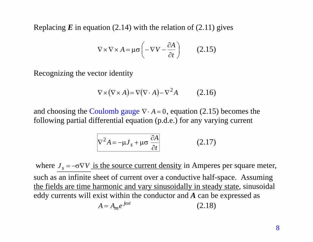
Replacing E in equation (2.14) with the relation of (2.11) gives

∂∂

−∇−=×∇×∇tAVA µσ (2.15)

Recognizing the vector identity

( ) ( ) AAA 2∇−⋅∇∇=×∇×∇ (2.16) and choosing the Coulomb gauge , equation (2.15) becomes the following partial differential equation (p.d.e.) for any varying current

0=⋅∇ A

tAJA s ∂

∂+−=∇ µ2 µσ (2.17)

where VJ s ∇−= σ is the source current density in Amperes per square meter, such as an infinite sheet of current over a conductive half-space. Assuming the fields are time harmonic and vary sinusoidally in steady state, sinusoidal eddy currents will exist within the conductor and A can be expressed as

tjeAA ω= m (2.18)

8

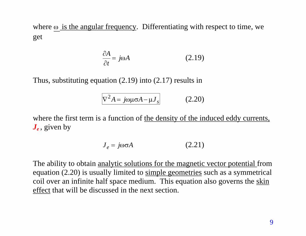
where ω is the angular frequency. Differentiating with respect to time, we get

AjtA

ω=∂∂ (2.19)

Thus, substituting equation (2.19) into (2.17) results in

sJAjA µωµσ −=∇2 (2.20) where the first term is a function of the density of the induced eddy currents, Je , given by

AjJe ωσ= (2.21) The ability to obtain analytic solutions for the magnetic vector potential from equation (2.20) is usually limited to simple geometries such as a symmetrical coil over an infinite half space medium. This equation also governs the skin effect that will be discussed in the next section.

9

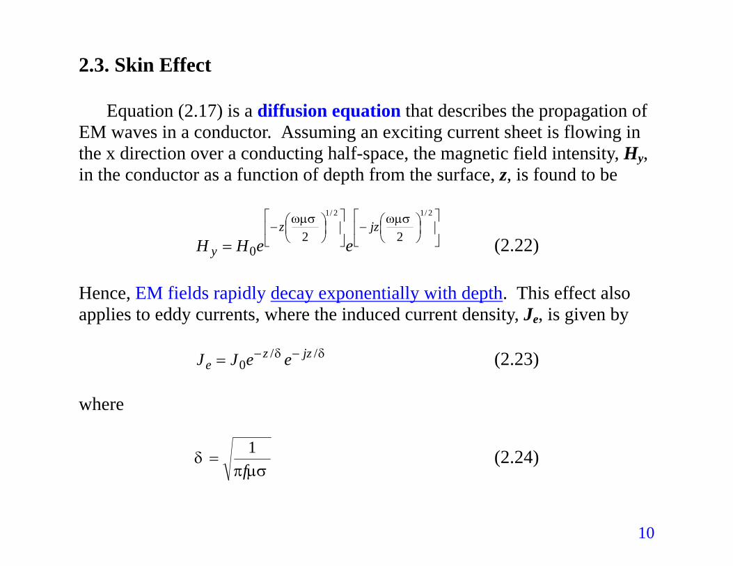
2.3. Skin Effect

Equation (2.17) is a diffusion equation that describes the propagation of EM waves in a conductor. Assuming an exciting current sheet is flowing in the x direction over a conducting half-space, the magnetic field intensity, Hy, in the conductor as a function of depth from the surface, z, is found to be

−

−

=

2/12/1

220

ωµσωµσ jzz

y eeHH (2.22) Hence, EM fields rapidly decay exponentially with depth. This effect also applies to eddy currents, where the induced current density, Je, is given by

δδ //0

jzze eeJJ −−= (2.23)

where

µσπδ

f1

= (2.24)

10

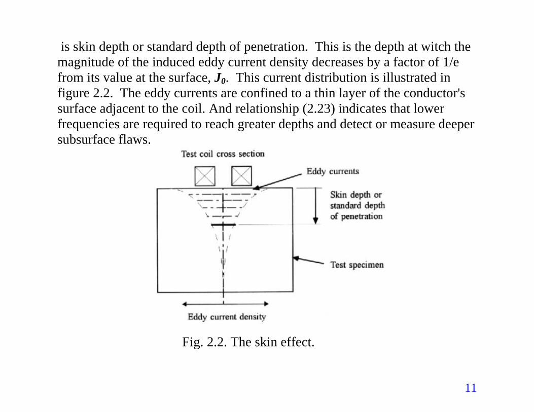
is skin depth or standard depth of penetration. This is the depth at witch the magnitude of the induced eddy current density decreases by a factor of 1/e from its value at the surface, J0. This current distribution is illustrated in figure 2.2. The eddy currents are confined to a thin layer of the conductor's surface adjacent to the coil. And relationship (2.23) indicates that lower frequencies are required to reach greater depths and detect or measure deeper subsurface flaws.

Fig. 2.2. The skin effect.

11

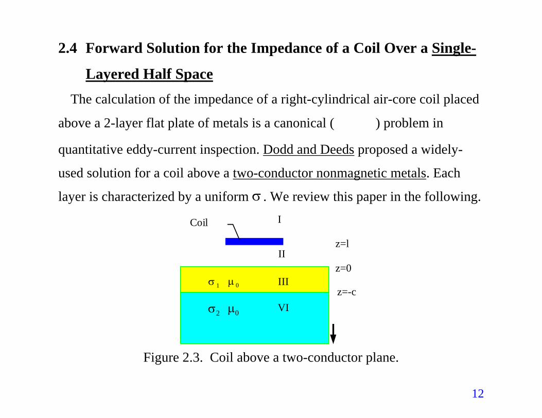
2.4 Forward Solution for the Impedance of a Coil Over a Single-

Layered Half Space The calculation of the impedance of a right-cylindrical air-core coil placed

above a 2-layer flat plate of metals is a canonical (標準的) problem in

quantitative eddy-current inspection. Dodd and Deeds proposed a widely-

used solution for a coil above a two-conductor nonmagnetic metals. Each

layer is characterized by a uniform . We review this paper in the following. σ

III

VI

I

IIz=0

z=-c

z=l

µ 0σ 1

µ0σ2

Coil

Figure 2.3. Coil above a two-conductor plane.

12

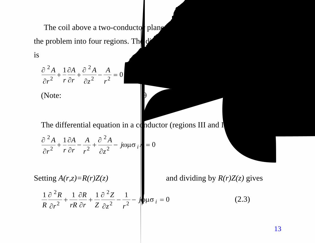
The coil above a two-conductor plane is shown in Fig. 2.3. We have divided

the problem into four regions. The differential equation in air (regions I and II)

is

0122

2

2

2=−++

rA

zA

rA

rrA

∂

∂∂∂

∂

∂. (圓柱座標) (2.1)

(Note: 由於對稱，所以與角度θ無關；空氣之σ=0，所以無 ) Aj iωµσ

The differential equation in a conductor (regions III and IV) is

012

2

22

2=−+−+ Aj

zA

rA

rA

rrA

iωµσ∂

∂∂∂

∂

∂ (2.2)

Setting A(r,z)=R(r)Z(z) （分離變數法）and dividing by R(r)Z(z) gives

0111122

2

2

2=−−++ ij

rzZ

ZrR

rRrR

Rωµσ

∂

∂∂∂

∂

∂ (2.3)

13

We write for the z dependence

ijconstz

ZZ

ωµσα∂

∂+== 2

2

21 , (2.4)

or

ii jzjz BeAeZ ωµσαωµσα −+ +=22 + . (2.5)

We define

ii jωµσαα +≡ 2 . (2.6)

Equation (2.3) then becomes

0111 222

2=+−+

∂∂

∂

∂

rrR

rRrR

Rα (2.7)

The is a first-order Bessel equation and has the solutions

( ) ( rDYrCJR αα 11 += ) (2.8)

Note: Bessel functions arise in solving differential equations for systems with

cylindrical symmetry.

14

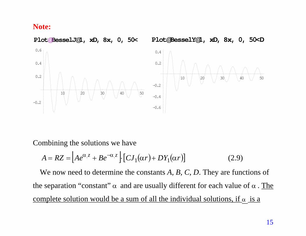
Note:

Plot BesselJ 1, x , x, 0, 50 Plot BesselY 1, x , x, 0, 50 @ @ D 8 < @ @ D 8 <D

10 20 30 40 50

-0.2

0.2

0.4

0.6

10 20 30 40 50

-0.6

-0.4

-0.2

0.2

0.4

Combining the solutions we have

[ ] ( ) ( )[ ]rDYrCJBeAeRZA zzii αααα

11 +⋅+== − (2.9)

We now need to determine the constants A, B, C, D. They are functions of

the separation “constant” and are usually different for each value of . α α The

complete solution would be a sum of all the individual solutions, if α is a

15

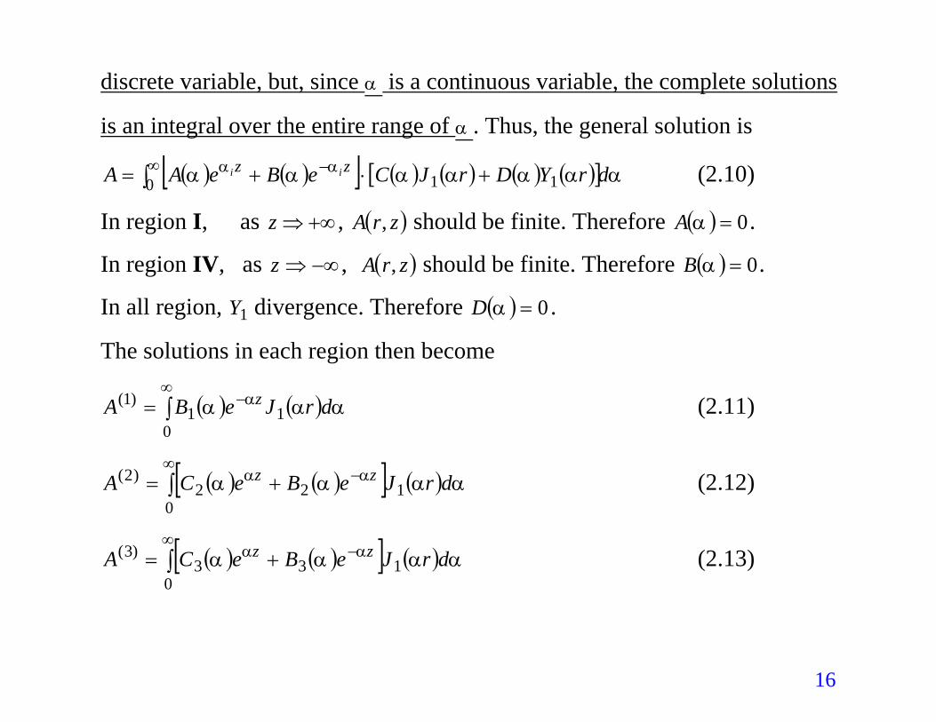
discrete variable, but, since α is a continuous variable, the complete solutions

is an integral over the entire range of α . Thus, the general solution is

[ ] r

D

( ) ( ) ( ) ( ) ( ) ( )[ ] ααααααα αα drYDJCeBeAA zz ii∫∞ − +⋅+= 0 11 (2.10)

In region I, as , ) should be finite. Therefore . +∞⇒z ( zrA , ( ) 0=αA

In region IV, as , ) should be finite. Therefore . −∞⇒z ( zrA , ( ) 0=αB

In all region, divergence. Therefore . 1Y ( ) 0=α

The solutions in each region then become

( ) ( )∫∞

−=0

11)1( ααα α drJeBA z (2.11)

( ) ( )[ ] ( )∫∞

−+=0

122)2( αααα αα drJeBeCA zz (2.12)

( ) ( )[ ] ( )∫∞

−+=0

133)3( αααα αα drJeBeCA zz (2.13)

16

( ) ( )∫∞

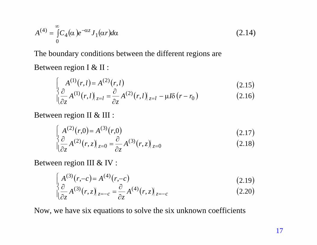
−=0

14)4( ααα α drJeCA z (2.14)

The boundary conditions between the different regions are

Between region I & II :

( ) ( )

( ) ( ) ( )

−−=

=

== 0)2()1(

)2()1(

,,

,,

rrIlrAz

lrAz

lrAlrA

lzlz δµ∂∂

∂∂

( )( )16.2

15.2

Between region II & III :

( ) ( )

( ) ( )

=

=

== 0)3(

0)2(

)3()2(

,,

0,0,

zz zrAz

zrAz

rArA

∂∂

∂∂

( )( )18.2

17.2

Between region III & IV :

( ) ( )

( ) ( )

=

−=−

−=−= czcz zrAz

zrAz

crAcrA

,,

,,)4()3(

)4()3(

∂∂

∂∂

( )( )20.2

19.2

Now, we have six equations to solve the six unknown coefficients

17

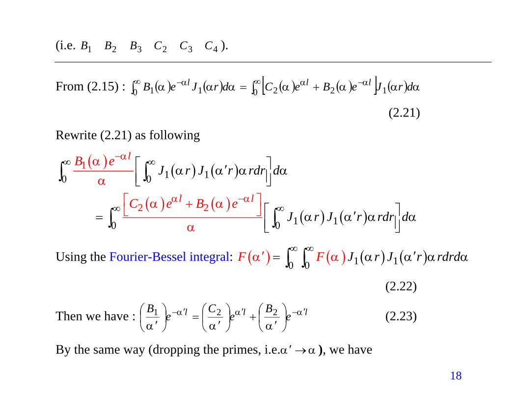
(i.e. ). 432321 CCCBBB

From (2.15) : ( ) ( ) ( ) ( )[ ] ( )∫∫∞ −∞ − += 0 1220 11 ααααααα ααα drJeBeCdrJeB lll

(2.21)

Rewrite (2.21) as following

( )

( ) ( )( ) ( )

2 2

l

l l

B e

C e B e

α

α α

α

α α

−

−∞ ∞

+ ∫ ∫

( ) ( )F α α=′

( ) ( )1 10 0

1 100

1 J r J r rdr d

J r J r rdr d

α α α α

α α

α

αα α

∞ ∞ ′

′=

∫ ∫

Using the Fourier-Bessel integral: ( ) ( )1 10 0J r J r r rF d dα α α α

∞ ∞′∫ ∫

(2.22)

Then we have : lll eB

eC

eB ααα

ααα′−′′−

′+

′=

′221 (2.23)

By the same way (dropping the primes, i.e. ), we have αα →′

18

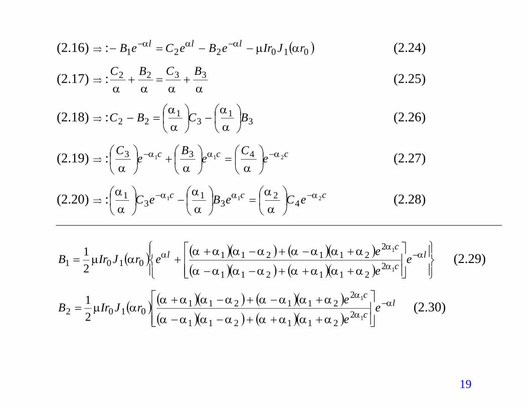
(2.16) ⇒ : ) (2.24) ( 010221 rJIreBeCeB lll αµααα −−=− −−

(2.17) ⇒ :αααα

3322 BCBC+=+ (2.25)

(2.18) ⇒ : 31

31

22 BCBC

−

=−

αα

αα (2.26)

(2.19) ⇒ : ccc eC

eB

eC

211 433 ααα

ααα−−

=

+

(2.27)

(2.20) ⇒ : ccc eCeBeC 2114

23

13

1 ααα

αα

αα

αα −−

=

−

(2.28)

( ) ( )( ) ( )( )( )( ) ( )( )

+++−−

+−+−++= − l

c

cl e

ee

erJIrB αα

αα

αααααααα

αααααααααµ

1

1

2211211

2211211

0101 21

(2.29)

( ) ( )( ) ( )( )( )( ) ( )( )

lc

ce

e

erJIrB α

α

α

αααααααα

αααααααααµ −

+++−−

+−+−+=

1

1

2211211

2211211

0102 21 (2.30)

19

( ) ( )( )( ) ( )( )

+++−−

−=

−

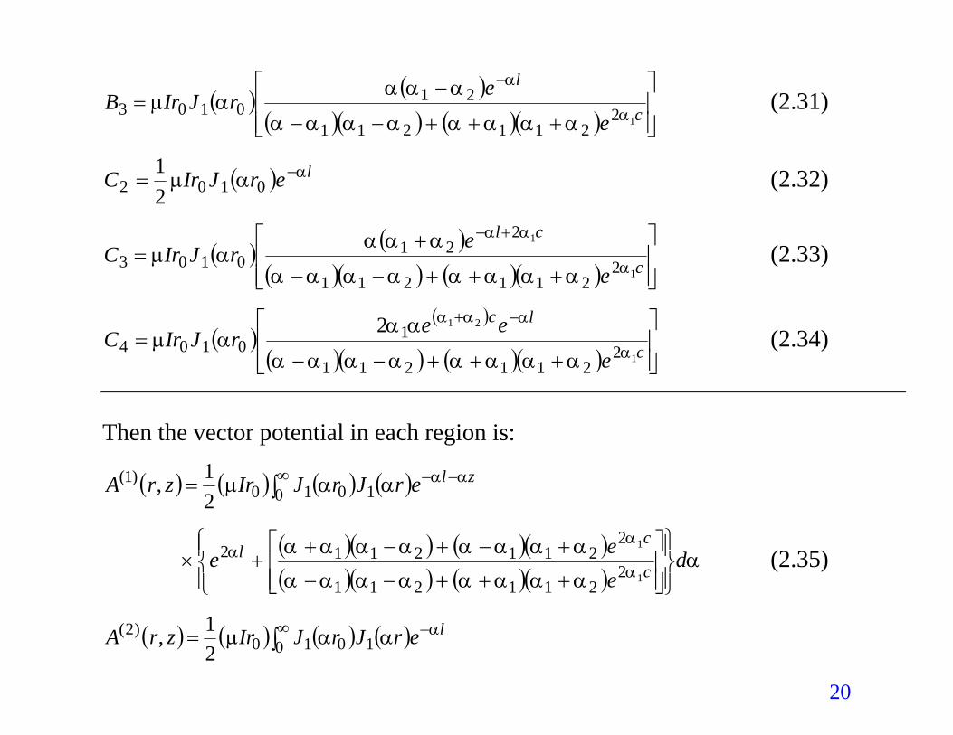
c

l

ee

rJIrB12

211211

210103 α

α

αααααααα

ααααµ (2.31)

( ) lerJIrC ααµ −= 0102 21 (2.32)

( ) ( )( )( ) ( )( )

+++−−

+=

+−

c

cl

e

erJIrC

1

1

2211211

221

0103 α

αα

αααααααα

ααααµ (2.33)

( )( )

( )( ) ( )( )

+++−−=

−+

c

lc

e

eerJIrC

1

21

2211211

10104

2α

ααα

αααααααα

αααµ (2.34)

Then the vector potential in each region is:

( ) ( ) ( ) ( )∫∞ −−= 0 1010

)1(21, zlerJrJIrzrA ααααµ

( )( ) ( )( )( )( ) ( )( )

ααααααααα

ααααααααα

αα d

eee c

cl

+++−−

+−+−++×

1

1

2211211

22112112 (2.35)

( ) ( ) ( ) ( )∫∞ −= 0 1010

)2(21, lerJrJIrzrA αααµ

20

( )( ) ( )( )( )( ) ( )( )

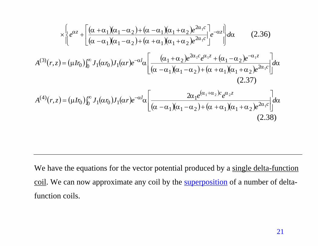
ααααααααα

αααααααα αα

αα de

eee z

c

cz

+++−−

+−+−++× −

1

1

2211211

2211211 (2.36)

( ) ( ) ( ) ( ) ( ) ( )( )( ) ( )( )

ααααααααα

αααααααµ α

αααα d

eeeeerJrJIrzrA c

zzcl∫

∞−

−

+++−−

−++= 0 2

211211

212

211010

)3(1

111

,

(2.37)

( ) ( ) ( ) ( )( )

( )( ) ( )( )α

αααααααα

ααααµ α

αααα d

eeeerJrJIrzrA c

zcl∫

∞+

−

+++−−= 0 2

211211

11010

)4(1

2212,

(2.38)

We have the equations for the vector potential produced by a single delta-function

coil. We can now approximate any coil by the superposition of a number of delta-

function coils.

21

( ) ( ) ( ) ( )∫ ∫∑∑ =====

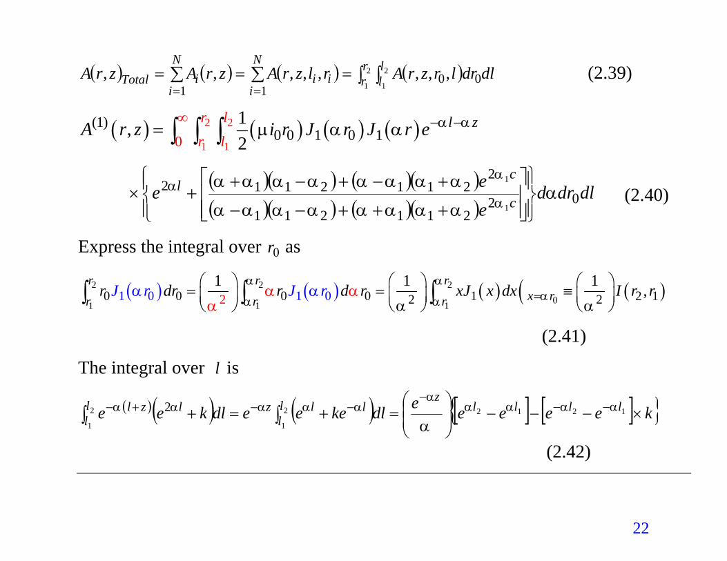
2

1

2

100

11,,,,,,,, r

rll

N

iii

N

iiTotal dldrlrzrArlzrAzrAzrA (2.39)

( ) ( ) ( ) ( )2

1 1

(1)0 0 1 0 10

,2r l

l zA r z i r J r J r e α αµ α α − −= ∫ ∫ 2 1r l∞∫

( )( ) ( )( )( )( ) ( )( )

dldrdeee c

cl

02211211

22112112

1

1

ααααααααα

ααααααααα

αα

+++−−

+−+−++× (2.40)

Express the integral over as 0r

( ) ( ) ( ) ( ( )2 2 201 1 1

0 0 0 0 1 2 121 0 12 0 21 1 1 ,

r r rx rr r r

r dr r d r xJ x dx I r rJ r J rα α

αα αα ααα αα

α=

= = ≡ ∫ ∫ ∫

(2.41)

The integral over is l

( )( ) ( ) [ ] [ ]{ }keeeeedlkeeedlkee llllz

ll

llzll

lzl ×−−−

=+=+ −−

−−−+− ∫∫ 12122

1

2

1

2 ααααα

ααααα

α

(2.42)

22

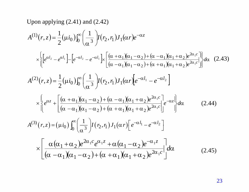
Upon applying (2.41) and (2.42)

( ) ( ) ( ) ( )∫∞ −

= 0 11230

)1( ,121, zerJrrIizrA αα

αµ

[ ] [ ] ( )( ) ( )( )( )( ) ( )( )

ααααααααα

ααααααααα

ααααα d

eeeeee c

cllll

+++−−

+−+−+×−−−× −−

1

11212

2211211

2211211 (2.43)

( ) ( ) ( ) ( )[ ]∫∞ −− −

= 0 11230

)2( 21,121, ll eerJrrIizrA ααα

αµ

( )( ) ( )( )( )( ) ( )( )

ααααααααα

αααααααα αα

αα de

eee z

c

cz

+++−−

+−+−++× −

1

1

2211211

2211211 (2.44)

( ) ( ) ( ) ( ) 1 2(3)0 2 1 130

1, , l lA r z i I r r J r e eα αµ αα

∞ − − = − ∫

( ) ( )( )( ) ( )( )

ααααααααα

ααααααα

αααd

eeee

c

zzc

+++−−

−++×

−

1

111

2211211

212

21 (2.45)

23

( ) ( ) ( ) ( )[ ]∫∞ −− −

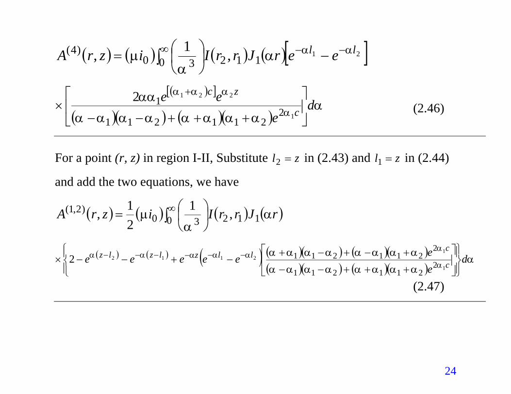
= 0 11230

)4( 21,1, ll eerJrrIizrA αααα

µ

( )[ ]

( )( ) ( )( )α

αααααααα

ααα

αααd

eee

c

zc

+++−−×

+

1

221

2211211

12 (2.46)

For a point (r, z) in region I-II, Substitute in (2.43) and in (2.44)

and add the two equations, we have

zl =2 zl =1

( ) ( ) ( ) ( )∫∞

= 0 11230

)2,1( ,121, rJrrIizrA α

αµ

( ) ( ) ( ) ( )( ) ( )( )( )( ) ( )( )

ααααααααα

ααααααααα

αααααα d

eeeeeee c

cllzlzlz

+++−−

+−+−+−+−−× −−−−−−

1

12112

2211211

22112112

(2.47)

24

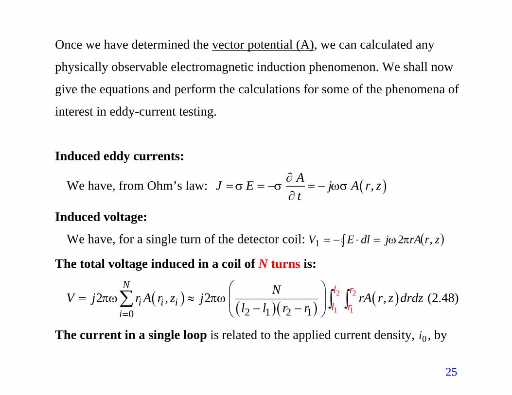
Once we have determined the vector potential (A), we can calculated any

physically observable electromagnetic induction phenomenon. We shall now

give the equations and perform the calculations for some of the phenomena of

interest in eddy-current testing.

Induced eddy currents:

We have, from Ohm’s law: ( ),AJ E j A rt

∂σ σ ωσ

∂= = − = − z

Induced voltage:

We have, for a single turn of the detector coil: ( )zrrAjdlEV ,21 πω=⋅−= ∫

The total voltage induced in a coil of N turns is:

( ) ( )( ) ( )2 2

1 12 1 2 102 , 2 ,

N

i i ii

l r

l rNV j r A r z j rA r z drd

l l r rπω πω

=

= ≈ − −

∑ ∫ ∫ z (2.48)

The current in a single loop is related to the applied current density, , by 0i

25

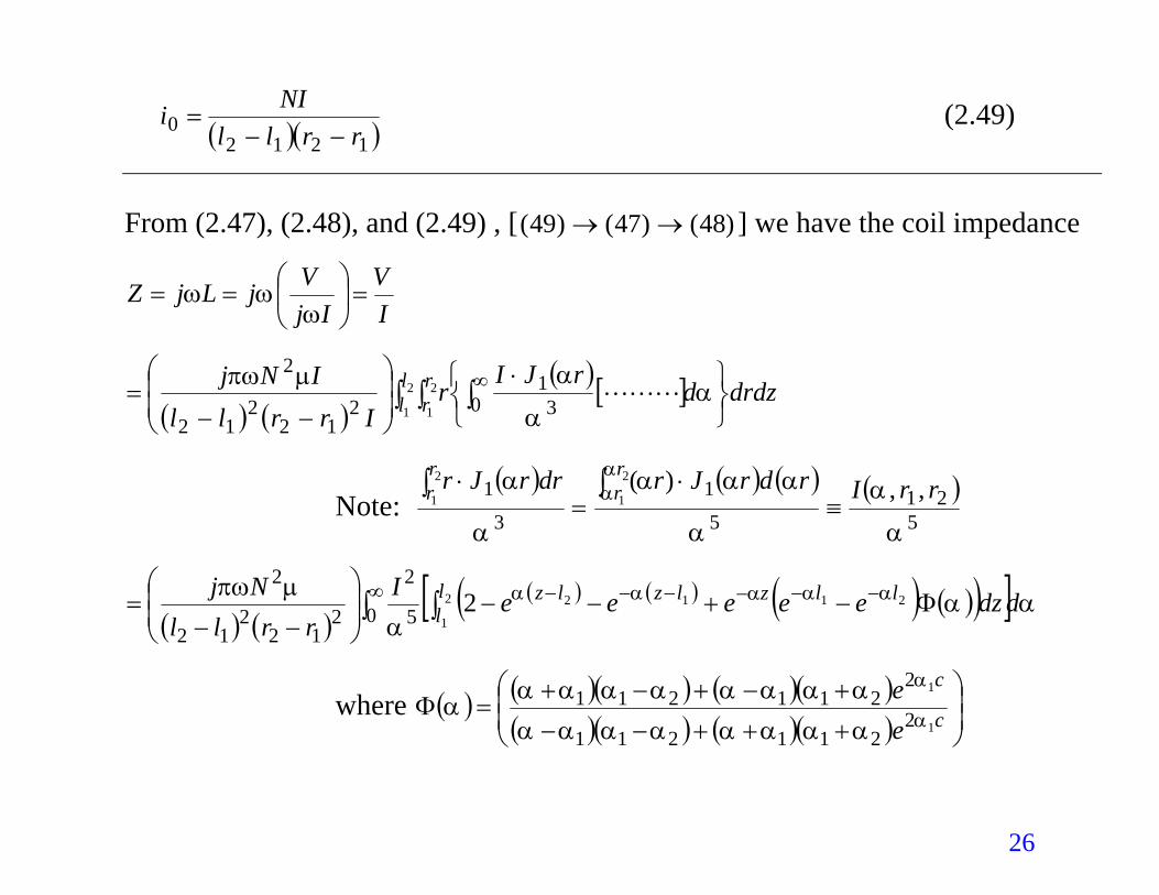
)( )( 1212

0 rrllNIi

−−= (2.49)

From (2.47), (2.48), and (2.49) , [ ] we have the coil impedance )48()47()49( →→

IV

IjVjLjZ =

==

ωωω

( ) ( )( )[ ]∫ ∫ ∫

⋅

−−= ∞2

1

2

1 0 31

212

212

2ll

rr drdzd

rJIr

IrrllINj

αα

αµπω

Note: ( ) ( ) ( ) ( )

521

51

31 ,,)(2

1

2

1

α

α

α

ααα

α

α αα rrIrdrJrdrrJr r

rrr ≡

⋅=

⋅ ∫∫

( ) ( )( ) ( ) ( ) ( )( )[ ] αα

αµπω ααααα ddzeeeeeI

rrllNj l

lllzlzlz∫ ∫

∞ −−−−−− Φ−+−−

−−= 0 5

2

212

212

22

1

21122

where ( ) ( )( ) ( )( )( )( ) ( )( )

+++−−

+−+−+= c

c

ee

1

1

2211211

2211211

α

α

αααααααα

αααααααααΦ

26

( ) ( )( ) ( ) ( ) ( ) ( )[ ]{ } αααα

α

ωπµ α dAellrrIrrll

Nj ll Φ+−+−−−

= −−−∞∫ 222,1

12112120

252

122

12

2

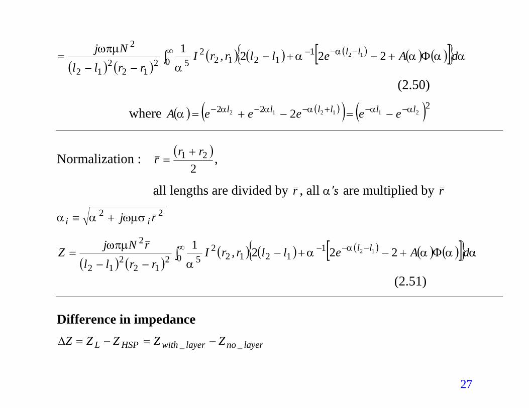
(2.50)

where ( ) ( )( ) ( )222 21121 2 llllll eeee αααααα −−+−−− −=−+= 2eA

Normalization : ( )2

21 rrr

+= ,

all lengths are divided by r , all are multiplied by sα ′ r 22 rj ii ωµσαα +≡

( ) ( )( ) ( ) ( ) ( ) ( )[ ]{ } αααα

α

ωπµ α dAellrrIrrll

rNjZ ll Φ+−+−−−

= −−−∞∫ 222,1

12112120

252

122

12

2

(2.51)

Difference in impedance

layernolayerwithHSPL ZZZZZ __ −=−=∆

27

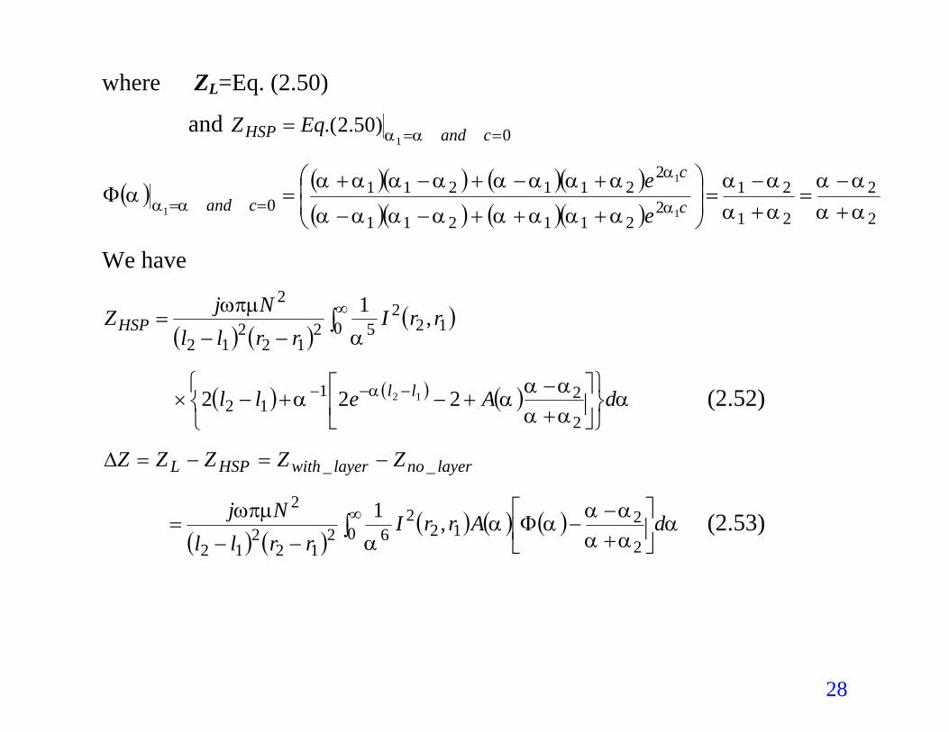
where ZL=Eq. (2.50)

and 01)50.2.( === candEq ααHSPZ

( ) ( )( ) ( )( )( )( ) ( )( ) 2

2

21

212

211211

2211211

0 1

1

1 αααα

αααα

αααααααα

ααααααααα

α

α

αα +−

=+−

=

+++−−

+−+−+=Φ == c

c

cand e

e

We have

( ) ( )( )120

252

122

12

2,1 rrI

rrllNjZHSP ∫

∞

−−=

αωπµ

( ) ( ) ( ) ααααα

αα α dAell ll

+−

+−+−× −−−

2

2112 222 12 (2.52)

layernolayerwithHSPL ZZZZZ __ −=−=∆

( ) ( )( ) ( ) ( ) α

αααα

ααα

ωπµ dArrIrrll

Nj

+−

−Φ−−

= ∫∞

2

2120

262

122

12

2,1 (2.53)

28

2.5 Review of Moulder et al.

In the following section, we will review the paper by Moulder et al. and

show how to apply Dodd and Deeds’ solutions to the eddy current

measurements.

Moulder et al. describe a robust method that uses eddy-current

measurements to determine the conductivity and thickness of aluminum and

copper layers on various substrate metals and that of free-standing foils of

aluminum, and the thickness and conductivity of free-standing foils of

aluminum. The impedance was measured for air-core and ferrite-core coils

either in the presence or the absence of the layer at frequencies ranging from

1 kHz to 1 MHz. The thickness and conductivity of the metallic layers were

inferred by matching the data taken with an air-core coil to the exact solution

derived Dodd and Deeds [5] using a least-squares norm. The inference was

absolute in the sense that no calibration was required. Both the thickness and

29

conductivity can be determined accurately and simultaneously if the ratio of

the layer thickness to the coil radius is between 0.20 and 0.50. For thinner

samples, one has to know the thickness to determine the conductivity, or vice

versa.

30

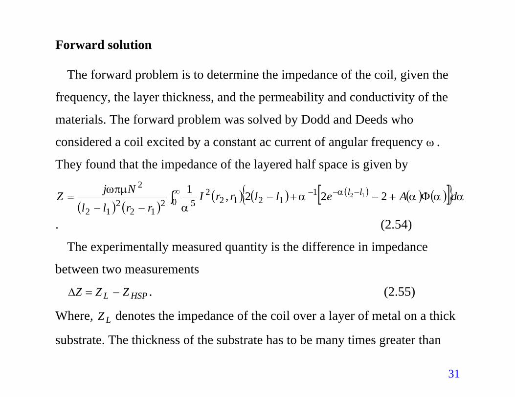
Forward solution

The forward problem is to determine the impedance of the coil, given the

frequency, the layer thickness, and the permeability and conductivity of the

materials. The forward problem was solved by Dodd and Deeds who

considered a coil excited by a constant ac current of angular frequency .

They found that the impedance of the layered half space is given by

ω

( ) ( )( ) ( ) ( ) ( ) ( )[ ]{ } αααα

α

ωπµ α dAellrrIrrll

NjZ ll Φ+−+−−−

= −−−∞∫ 222,1

12112120

252

122

12

2

. (2.54)

The experimentally measured quantity is the difference in impedance

between two measurements

HSPL ZZZ −=∆ . (2.55)

Where, denotes the impedance of the coil over a layer of metal on a thick

substrate. The thickness of the substrate has to be many times greater than LZ

31

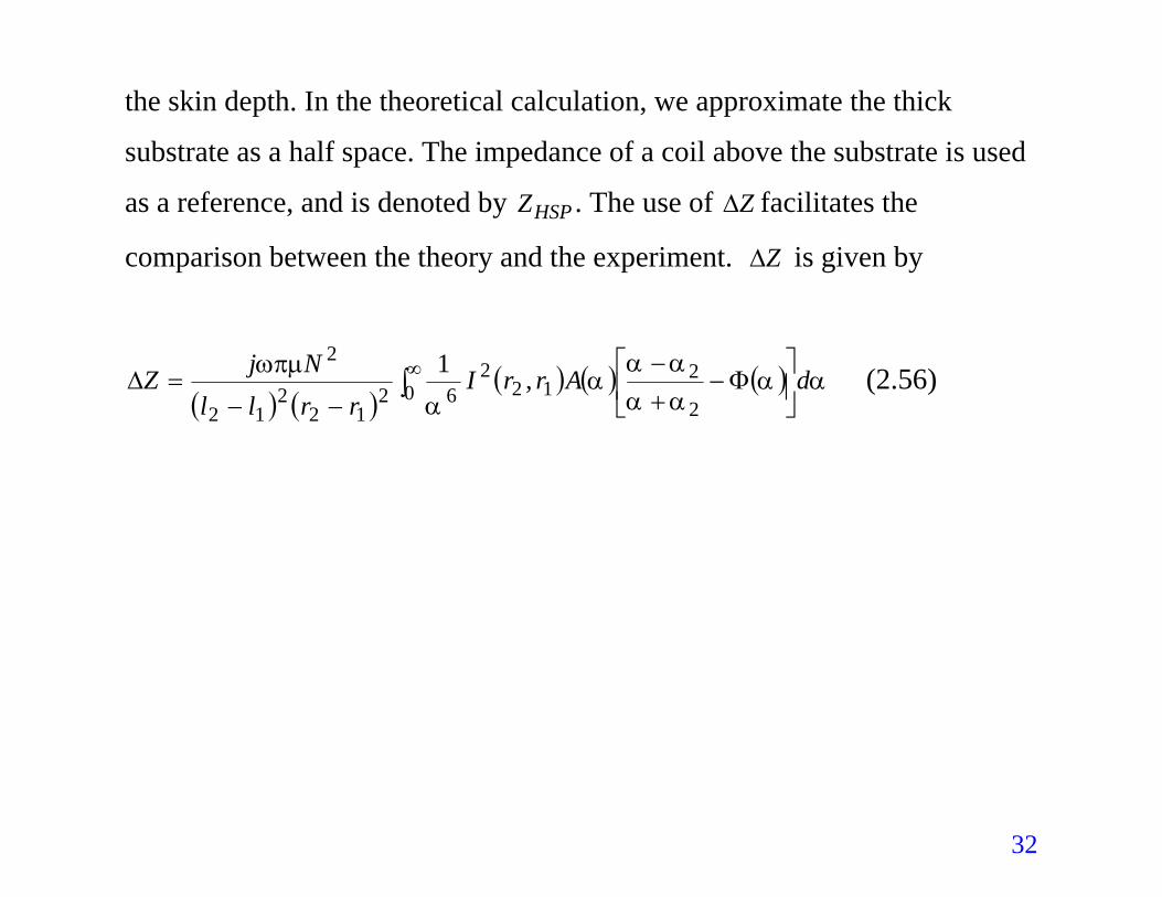
the skin depth. In the theoretical calculation, we approximate the thick

substrate as a half space. The impedance of a coil above the substrate is used

as a reference, and is denoted by . The use of facilitates the

comparison between the theory and the experiment. is given by HSPZ Z∆

∆Z

( )αΦAr12 ,

( ) ( )( ) ( ) α

αααα

αα

ωπµ drIrrll

NjZ

−

+−

−−=∆ ∫

∞

2

20

262

122

12

2 1 (2.56)

32

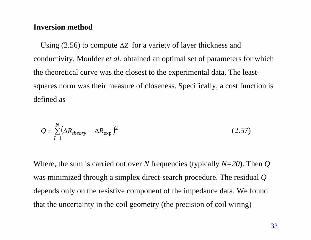
Inversion method

Using (2.56) to compute for a variety of layer thickness and

conductivity, Moulder et al. obtained an optimal set of parameters for which

the theoretical curve was the closest to the experimental data. The least-

squares norm was their measure of closeness. Specifically, a cost function is

defined as

Z∆

( )∑=

∆−∆≡N

Itheory RRQ

1

2exp (2.57)

Where, the sum is carried out over N frequencies (typically N=20). Then Q

was minimized through a simplex direct-search procedure. The residual Q

depends only on the resistive component of the impedance data. We found

that the uncertainty in the coil geometry (the precision of coil wiring)

33

strongly affects the reactive (inductive) components of the impedance.

Consequently, they focused the inversion efforts on , which seemed to be

less sensitive to these model errors.

R∆

34