Embed Size (px)
Citation preview
The Islamic University of Gaza
Faculty of Engineering
Civil Engineering Department
Numerical AnalysisECIV 3306
Chapter 18
Interpolation
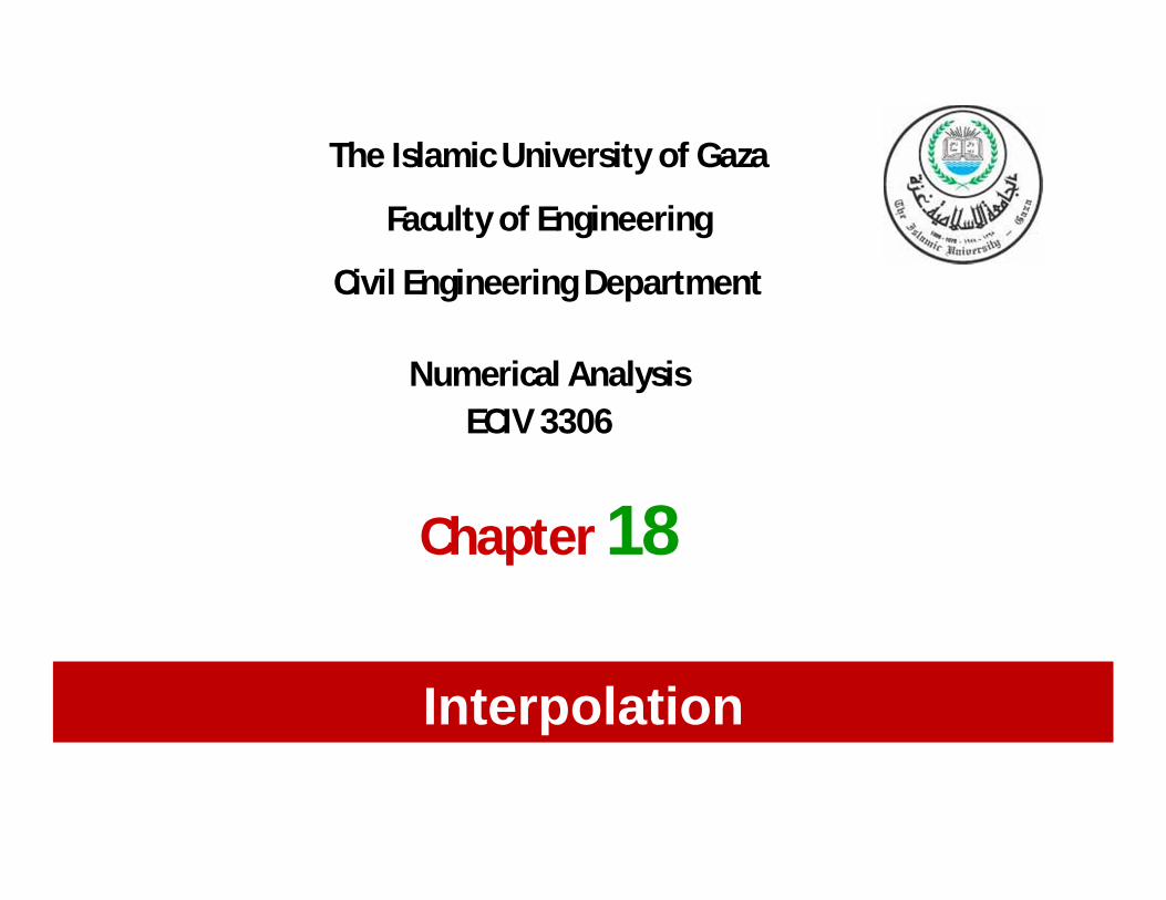
IntroductionThe most common method for Estimation ofintermediate values between precise data pointsis polynomial interpolation. :
Polynomial interpolation is used when the pointdetermined are very precise. The curverepresenting the behavior has to pass throughevery point.There is one and only one nth-order polynomialthat fits n+1 points
nn xaxaxaaxf 2
210)(
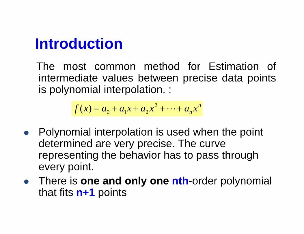
Introduction
First order (linear) 3rd order (cubic)2nd order (quadratic)
n = 2 n = 3 n = 4
Introduction
There are a variety of mathematical formats inwhich this polynomial can be expressed:
The Newton polynomial (sec. 18.1)
The Lagrange polynomial (sec. 18.2)
Lagrange Interpolating Polynomials
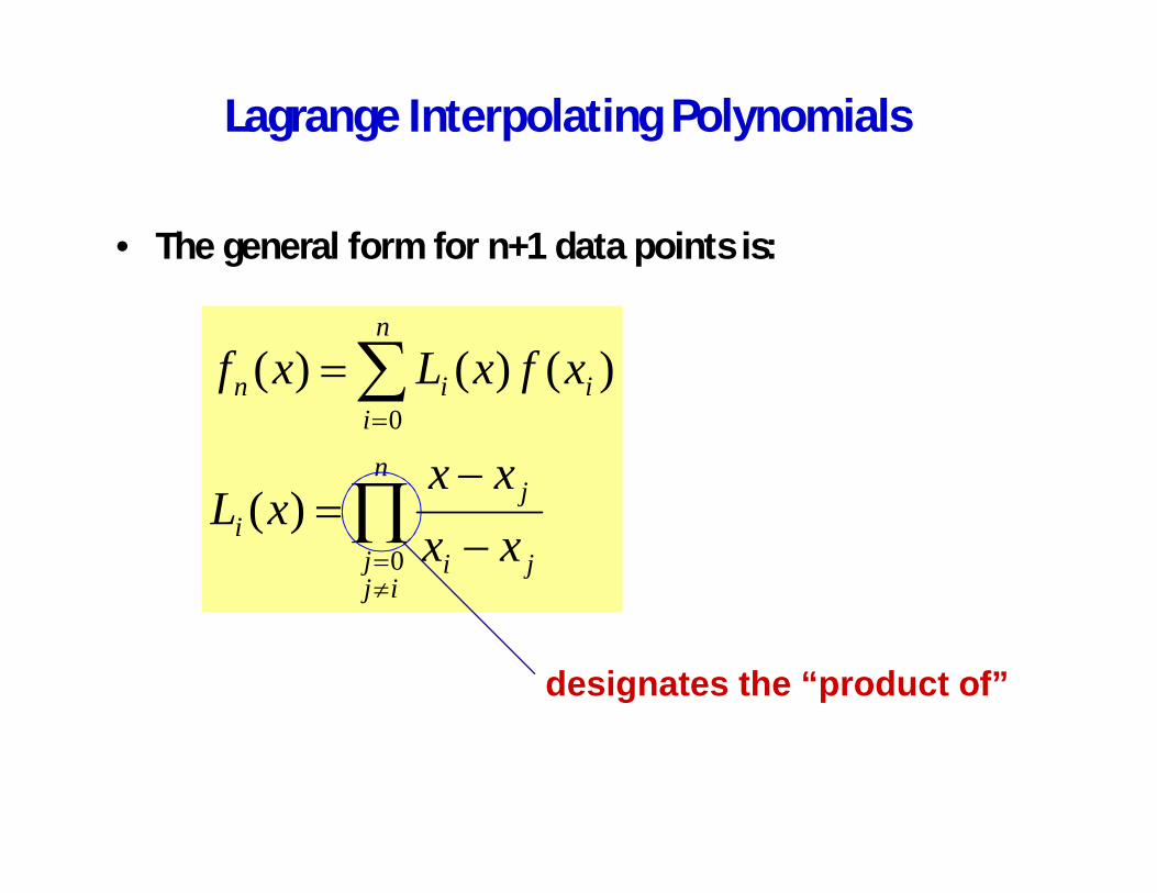
• The general form for n+1 data points is:
n
ijj ji
ji
n
iiin
xxxx
xL
xfxLxf
0
0
)(
)()()(
designates the “product of”
Lagrange Interpolating Polynomials
)()()( 101
00
10
11 xf
xxxxxf
xxxxxf
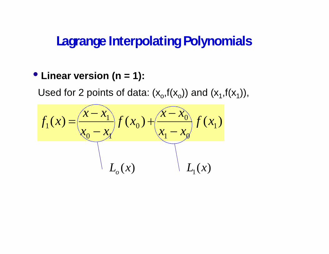
• Linear version (n = 1):Used for 2 points of data: (xo,f(xo)) and (x1,f(x1)),
)(xLo )(1 xL
Lagrange Interpolating Polynomials
1,)(1 jxL
)(
)(
)()(
21202
10
12101
20
02010
212
xfxxxx
xxxx
xfxxxxxxxx
xfxxxx
xxxxxf
2,)(2 jxL
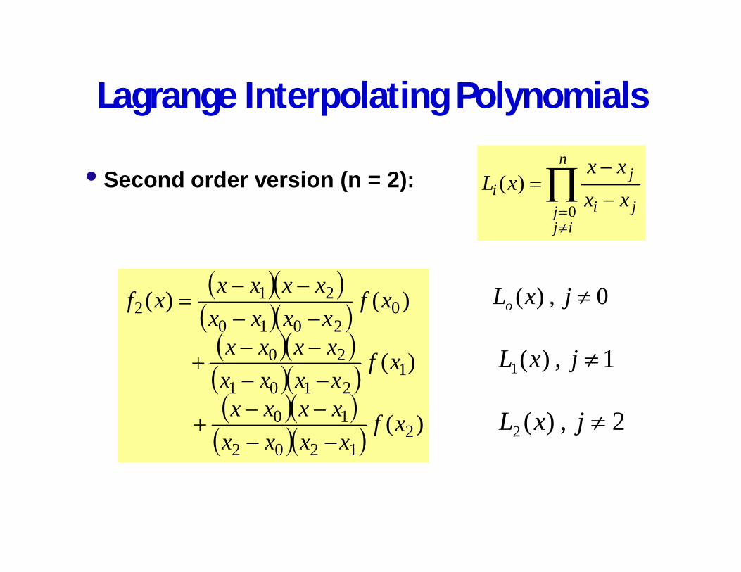
• Second order version (n = 2):
0,)( jxLo
n
ijj ji
ji xx
xxxL
0
)(
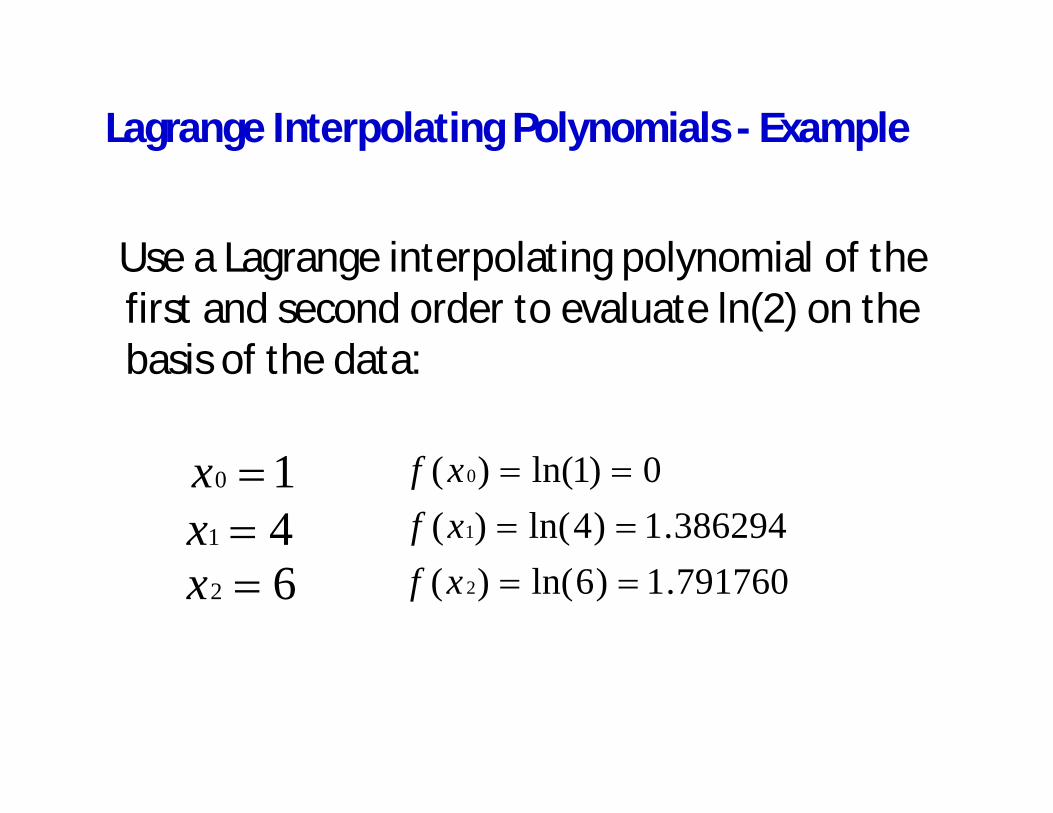
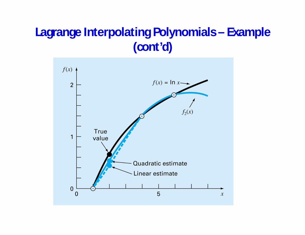
Lagrange Interpolating Polynomials - Example
Use a Lagrange interpolating polynomial of thefirst and second order to evaluate ln(2) on thebasis of the data:
10x 0)1ln()( 0xf
41x62x
386294.1)4ln()( 1xf791760.1)6ln()( 2xf
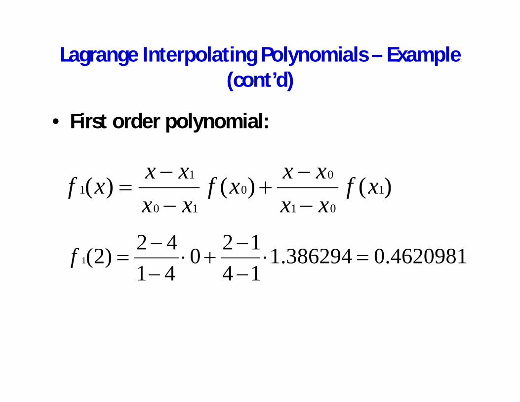
Lagrange Interpolating Polynomials – Example(cont’d)
• First order polynomial:
)()()( 101
00
10
11 xf
xxxxxf
xxxxxf
4620981.0386294.114120
4142)2(1f
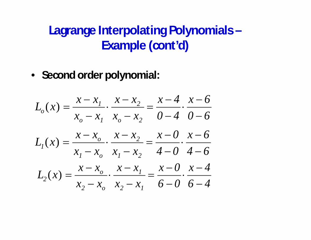
Lagrange Interpolating Polynomials –Example (cont’d)
• Second order polynomial:
606x
404x
xxxx
xxxxxL
2o
2
1o
1o )(
646x
040x
xxxx
xxxxxL
21
2
o1
o1 )(
464x
060x
xxxx
xxxxxL
12
1
o2
o2 )(
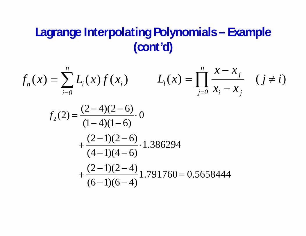
Lagrange Interpolating Polynomials – Example(cont’d)
5658444.0791760.1)46)(16()42)(12(
386294.1)64)(14()62)(12(
0)61)(41()62)(42()2(2f
n
0iiin xfxLxf )()()( )()( ij
xxxx
xLn
0j ji
ji
Lagrange Interpolating Polynomials – Example(cont’d)
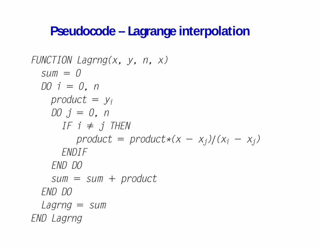
Pseudocode – Lagrange interpolation
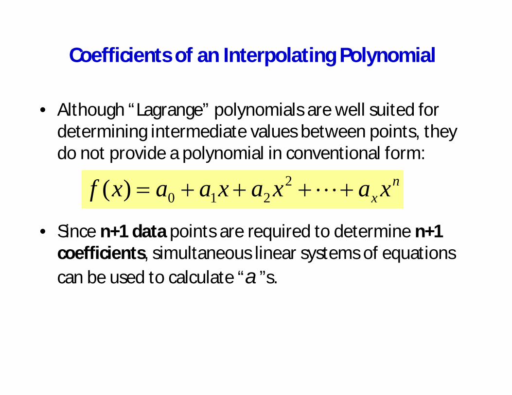
Coefficients of an Interpolating Polynomial
• Although “Lagrange” polynomials are well suited fordetermining intermediate values between points, theydo not provide a polynomial in conventional form:
• Since n+1 data points are required to determine n+1coefficients, simultaneous linear systems of equationscan be used to calculate “a”s.
nx xaxaxaaxf 2
210)(
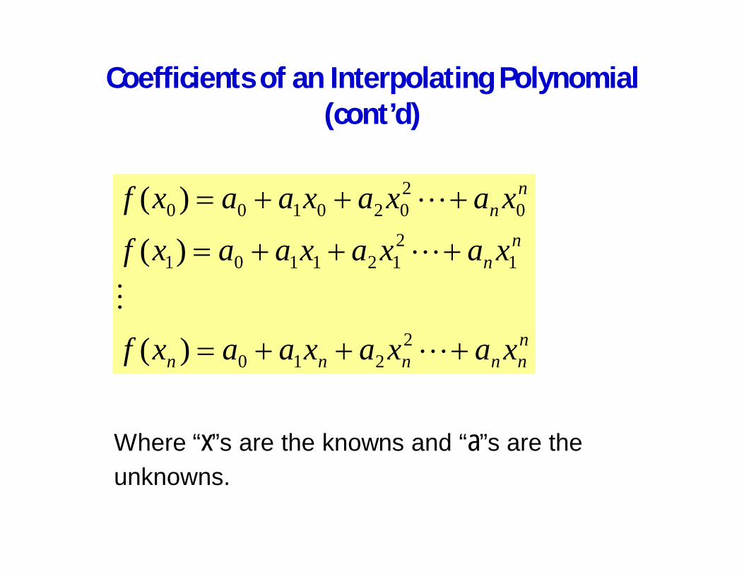
Coefficients of an Interpolating Polynomial(cont’d)
nnnnnn
nn
nn
xaxaxaaxf
xaxaxaaxfxaxaxaaxf
2210
12121101
02020100
)(
)(
)(
Where “x”s are the knowns and “a”s are theunknowns.
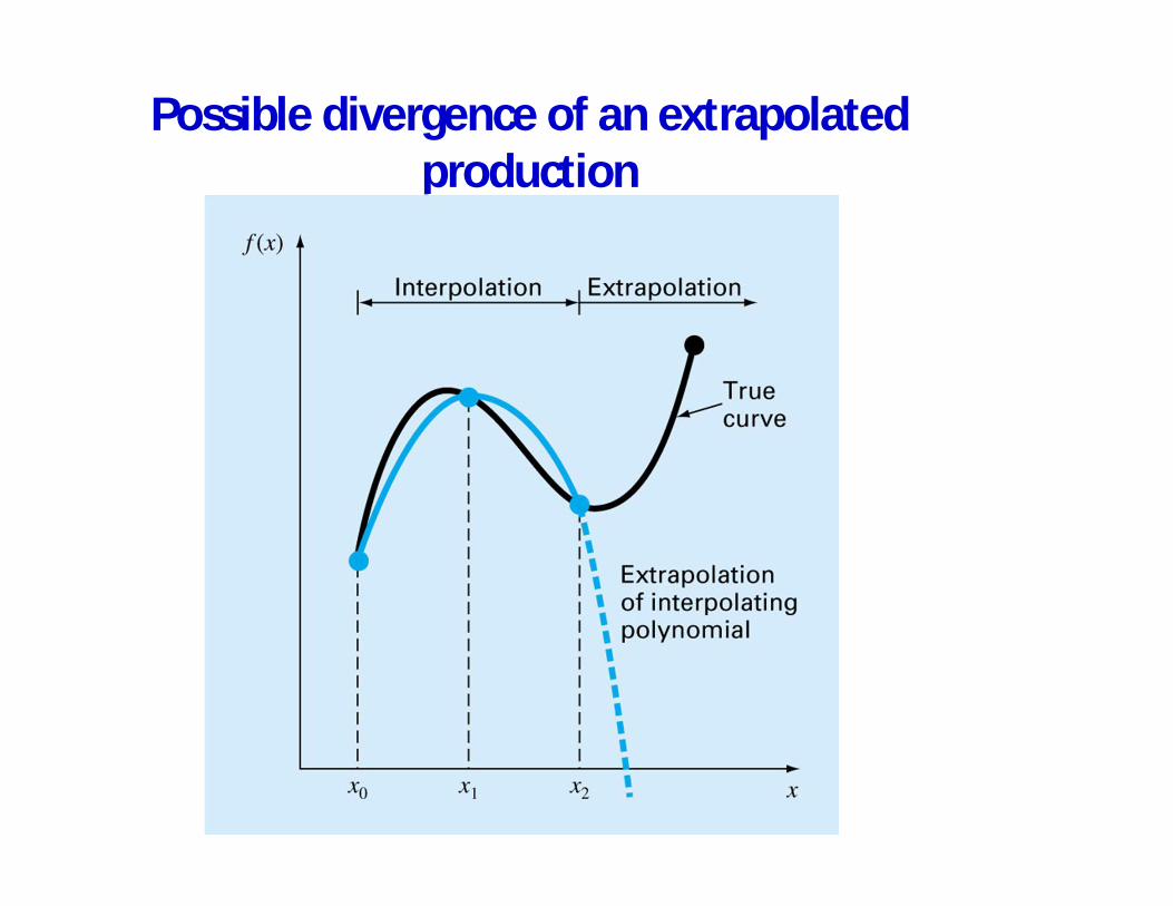
Possible divergence of an extrapolatedproduction
Spline Interpolation
• Polynomials are the most common choice ofinterpolants.
• There are cases where polynomials can lead toerroneous results because of round off error andovershoot.
• Alternative approach is to apply lower-orderpolynomials to subsets of data points. Suchconnecting polynomials are called spline functions.
18
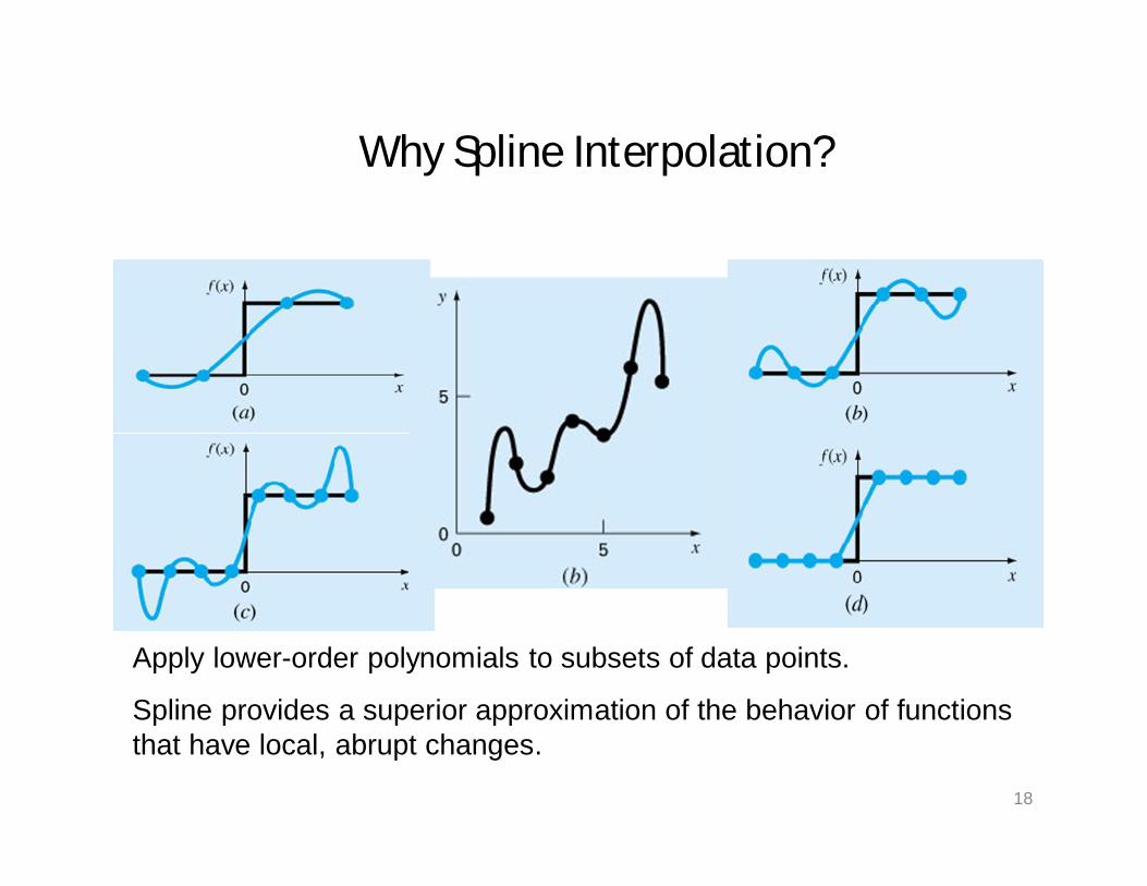
Why Spline Interpolation?
Apply lower-order polynomials to subsets of data points.
Spline provides a superior approximation of the behavior of functionsthat have local, abrupt changes.
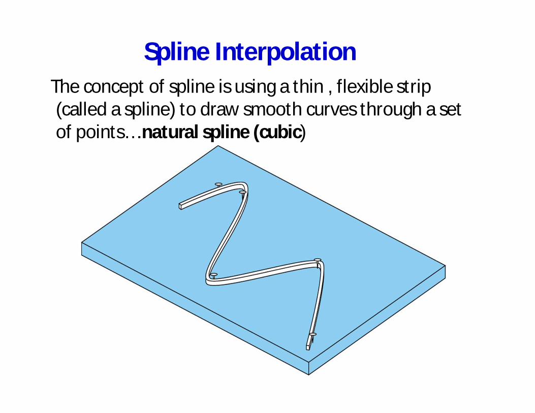
Spline InterpolationThe concept of spline is using a thin , flexible strip(called a spline) to draw smooth curves through a setof points….natural spline (cubic)
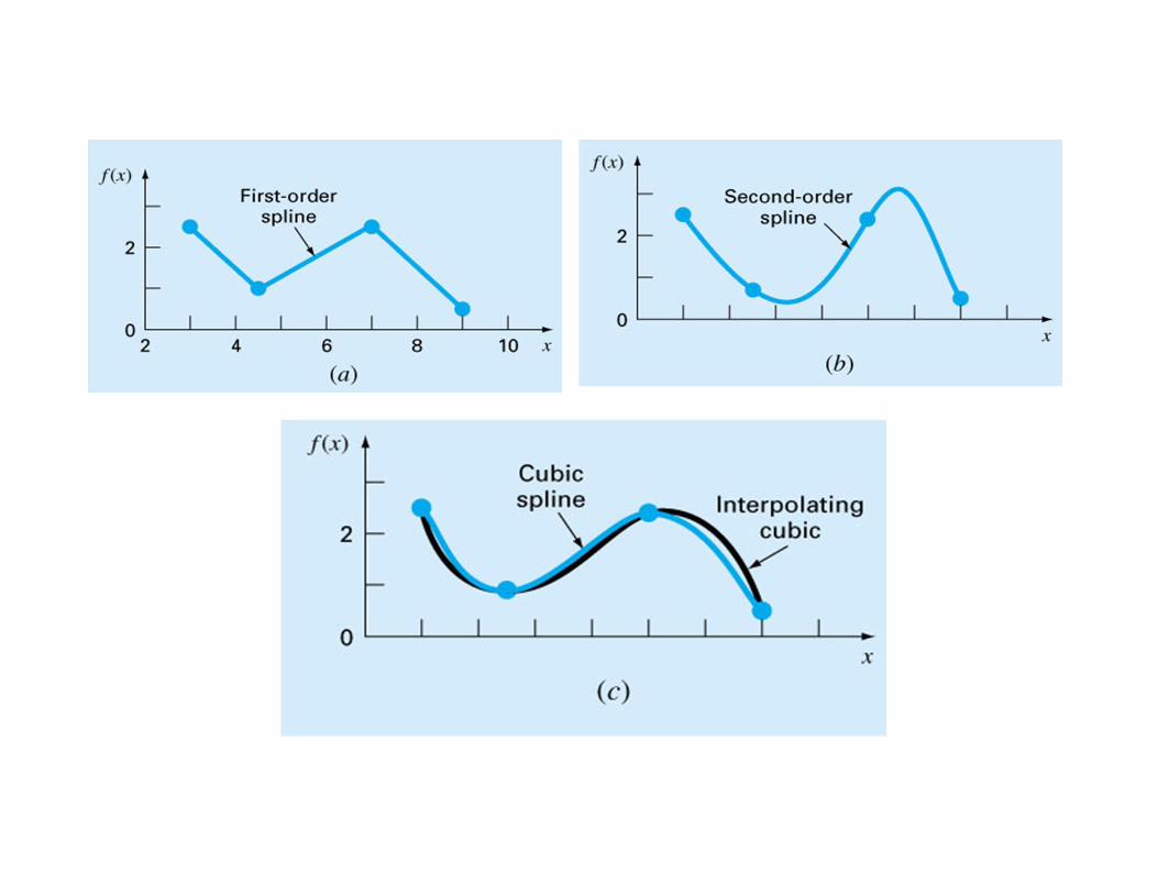
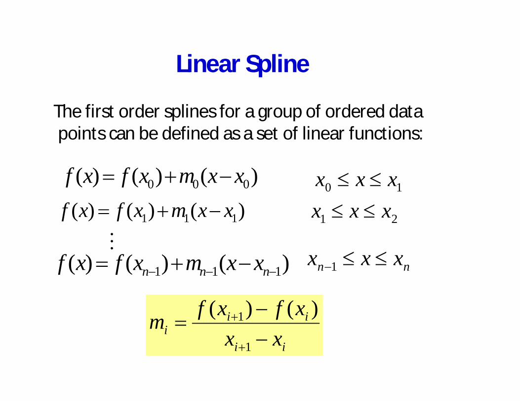
Linear Spline
The first order splines for a group of ordered datapoints can be defined as a set of linear functions:
ii
iii xx
xfxfm1
1 )()(
)()()( 000 xxmxfxf10 xxx
)()()( 111 xxmxfxf 21 xxx
)()()( 111 nnn xxmxfxf nn xxx 1
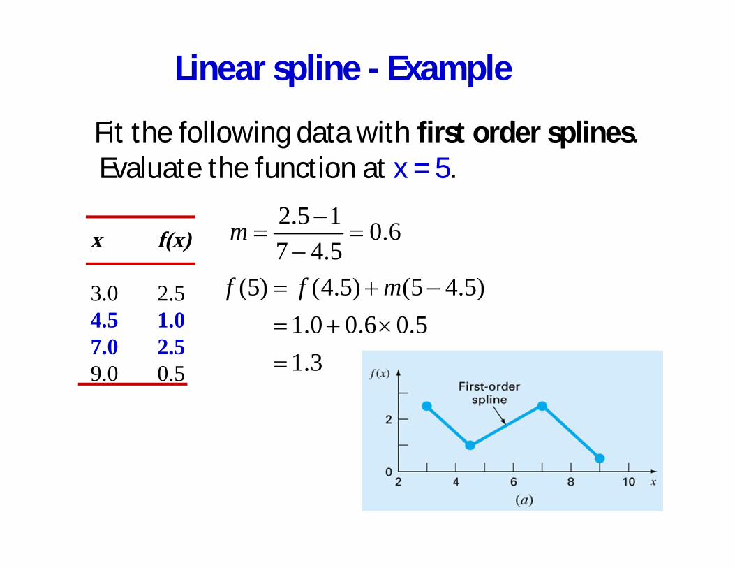
Linear spline - Example
Fit the following data with first order splines.Evaluate the function at x = 5.
x f(x)
3.0 2.54.5 1.07.0 2.59.0 0.5
6.05.4715.2m
3.15.06.00.1
)5.45()5.4()5( mff
Linear Spline
• The main disadvantage of linear spline is that they arenot smooth. At the data points where 2 splines meetscalled (a knot), the slope changes abruptly.
• The first derivative of the function is discontinuous atthese points.
• Using higher order polynomial splines ensuresmoothness at the knots by equating derivatives atthese points.
Quadratic Splines
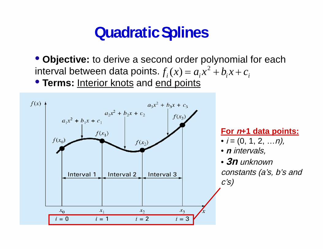
iiii cxbxaxf 2)(• Objective: to derive a second order polynomial for eachinterval between data points.• Terms: Interior knots and end points
For n+1 data points:• i = (0, 1, 2, …n),• n intervals,• 3n unknownconstants (a’s, b’s andc’s)
Quadratic Splines
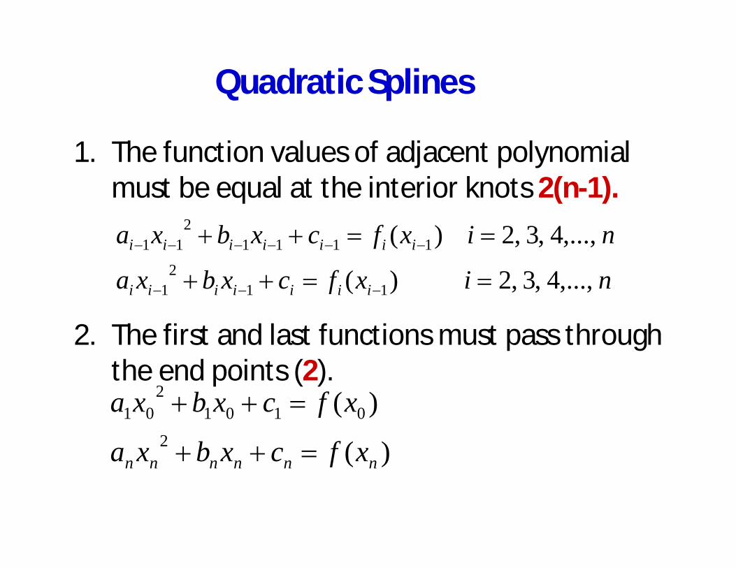
1. The function values of adjacent polynomialmust be equal at the interior knots 2(n-1).
2. The first and last functions must pass throughthe end points (2).
nixfcxbxa
nixfcxbxa
iiiiiii
iiiiiii
,...,4,3,2)(
,...,4,3,2)(
112
1
11112
11
)(
)(2
01012
01
nnnnnn xfcxbxa
xfcxbxa
Quadratic Splines
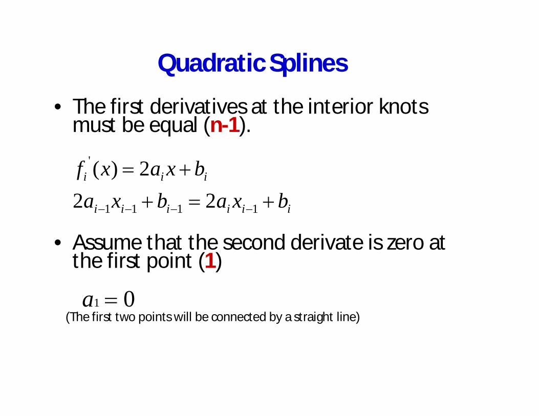
• The first derivatives at the interior knotsmust be equal (n-1).
• Assume that the second derivate is zero atthe first point (1)
(The first two points will be connected by a straight line)
iiiiii
iii
bxabxabxaxf
1111
'
222)(
01a
Quadratic Splines - Example
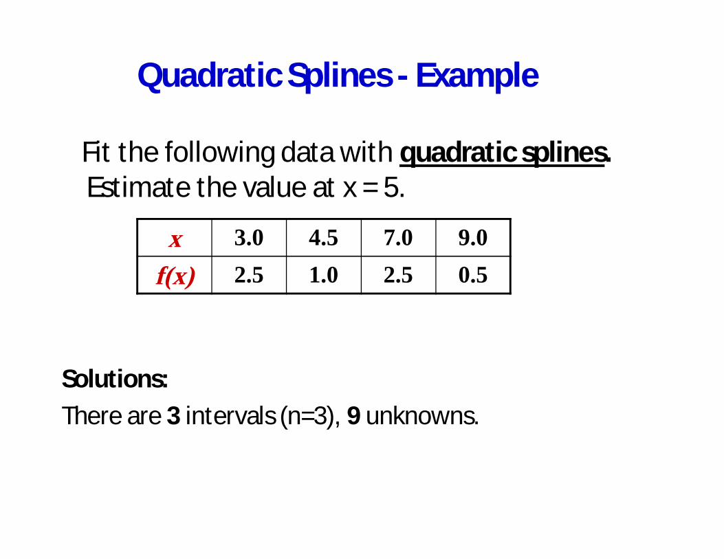
Fit the following data with quadratic splines.Estimate the value at x = 5.
Solutions:There are 3 intervals (n=3), 9 unknowns.
x 3.0 4.5 7.0 9.0f(x) 2.5 1.0 2.5 0.5
Quadratic Splines - Example
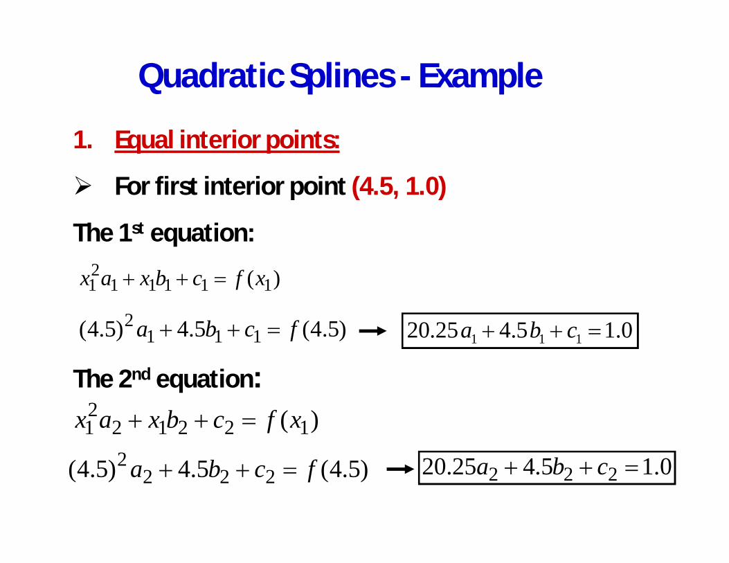
1. Equal interior points:
For first interior point (4.5, 1.0)
The 1st equation:
The 2nd equation:)( 12212
21 xfcbxax
0.15.425.20 111 cba
)( 1111121 xfcbxax
)5.4(5.4)5.4( 1112 fcba
0.15.425.20 222 cba)5.4(5.4)5.4( 2222 fcba
Quadratic Splines - Example
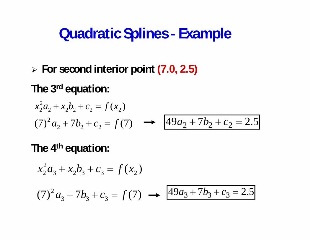
For second interior point (7.0, 2.5)
The 3rd equation:
The 4th equation:
5.2749 222 cba
5.2749 333 cba
)( 2222222 xfcbxax
)7(7)7( 2222 fcba
)( 2332322 xfcbxax
)7(7)7( 3332 fcba
Quadratic Splines - Example
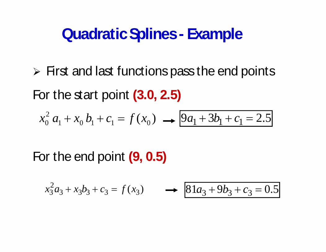
First and last functions pass the end points
For the start point (3.0, 2.5)
For the end point (9, 0.5)
5.239 111 cba
5.0981 333 cba
)( 0110120 xfcbxax
)( 3333323 xfcbxax
Quadratic Splines - Example
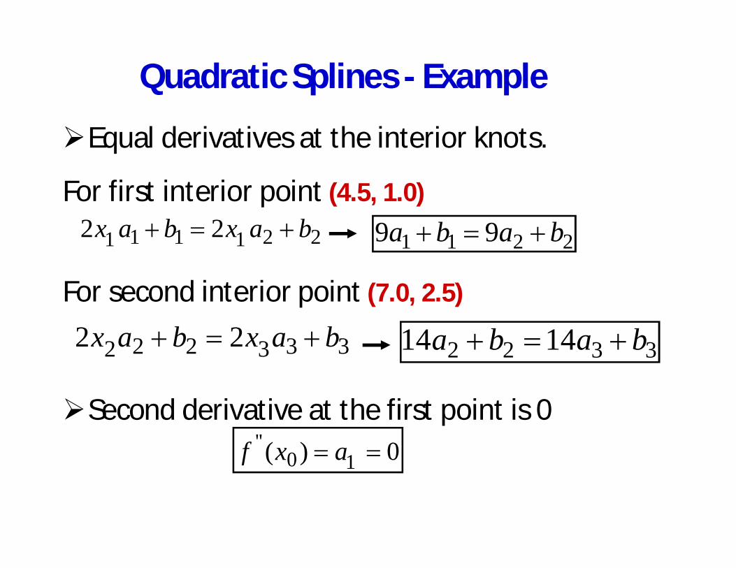
Equal derivatives at the interior knots.
For first interior point (4.5, 1.0)
For second interior point (7.0, 2.5)
Second derivative at the first point is 00)( 10
'' axf
2211 99 baba221111 22 baxbax
3322 1414 baba333222 22 baxbax
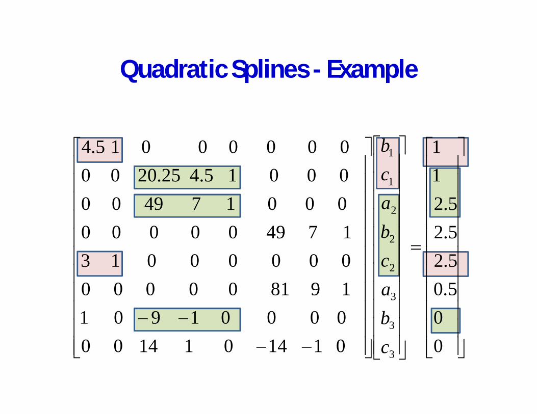
Quadratic Splines - Example
00
5.05.25.25.2
11
01140114000000190119810000000000013174900000
00017490000015.425.200000000015.4
3
3
3
2
2
2
1
1
cbacbacb
Quadratic Splines - Example
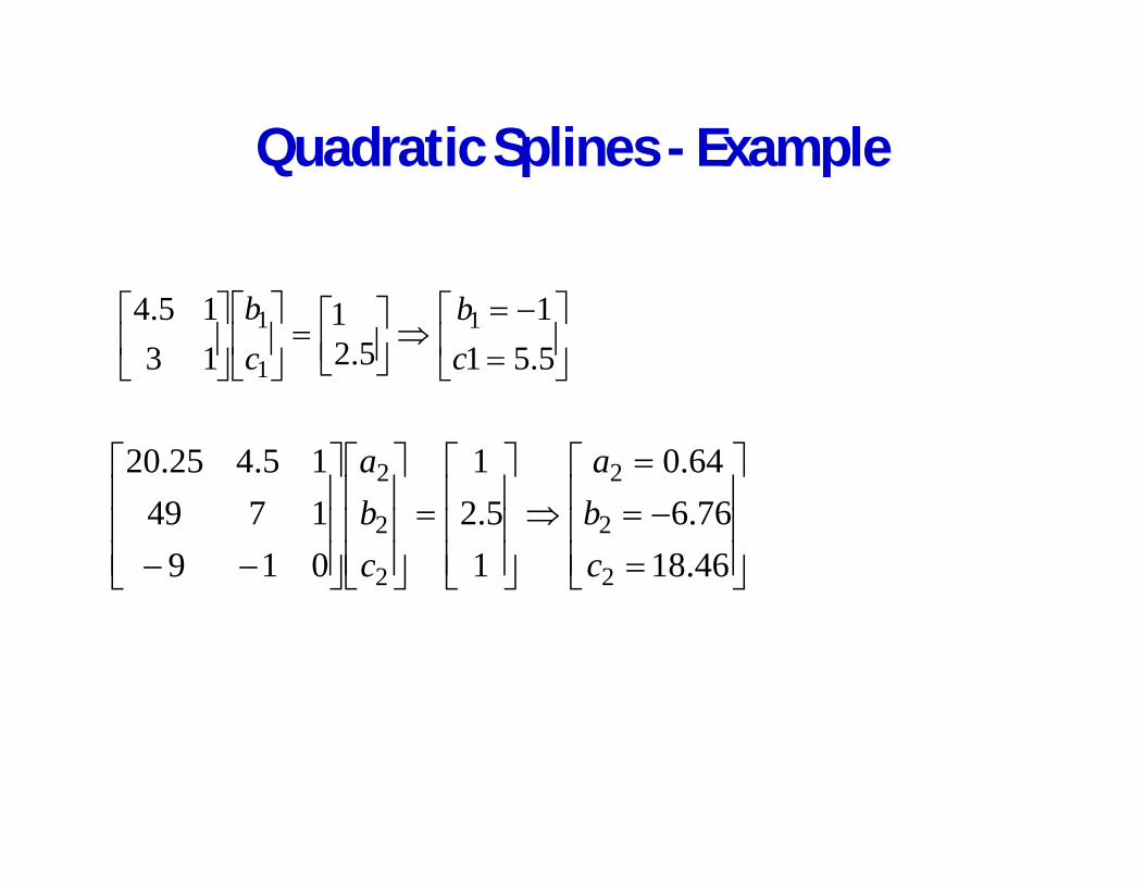
5.511
5.21
1315.4 1
1
1
cb
cb
46.1876.664.0
15.2
1
019174915.425.20
2
2
2
2
2
2
cba
cba
Quadratic Splines - Example
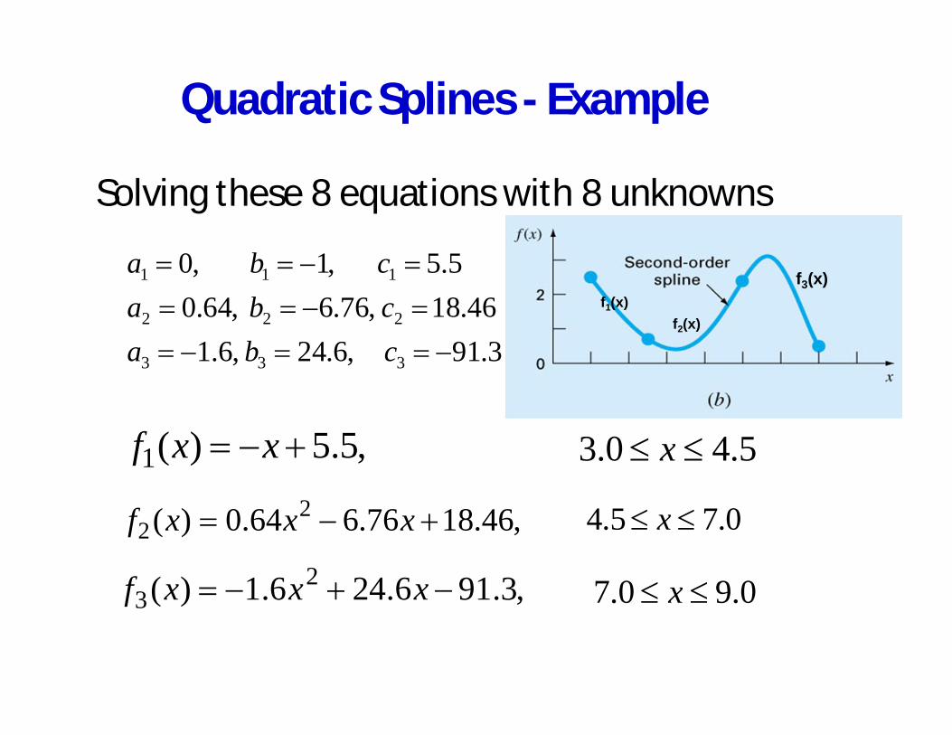
Solving these 8 equations with 8 unknowns
3.91,6.24,6.146.18,76.6,64.0
5.5,1,0
333
222
111
cbacbacba
,5.5)(1 xxf 5.40.3 x
,46.1876.664.0)( 22 xxxf 0.75.4 x
,3.916.246.1)( 23 xxxf 0.90.7 x
f1(x)f2(x)
f3(x)
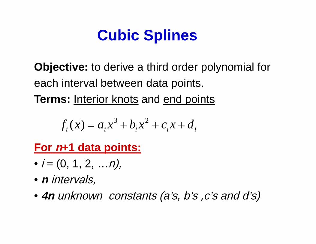
Cubic Splines
iiiii dxcxbxaxf 23)(
Objective: to derive a third order polynomial foreach interval between data points.Terms: Interior knots and end points
For n+1 data points:• i = (0, 1, 2, …n),• n intervals,• 4n unknown constants (a’s, b’s ,c’s and d’s)
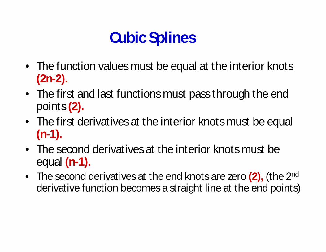
Cubic Splines
• The function values must be equal at the interior knots(2n-2).
• The first and last functions must pass through the endpoints (2).
• The first derivatives at the interior knots must be equal(n-1).
• The second derivatives at the interior knots must beequal (n-1).
• The second derivatives at the end knots are zero (2), (the 2nd
derivative function becomes a straight line at the end points)
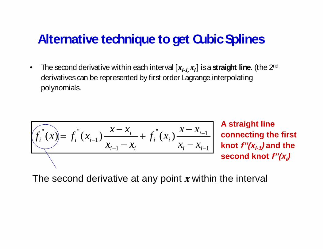
Alternative technique to get Cubic Splines
• The second derivative within each interval [xi-1, xi ] is a straight line. (the 2nd
derivatives can be represented by first order Lagrange interpolatingpolynomials.
1
1''
11
'''' )()()(ii
iii
ii
iiii xx
xxxfxx
xxxfxfA straight lineconnecting the firstknot f’’(xi-1) and thesecond knot f’’(xi)
The second derivative at any point x within the interval
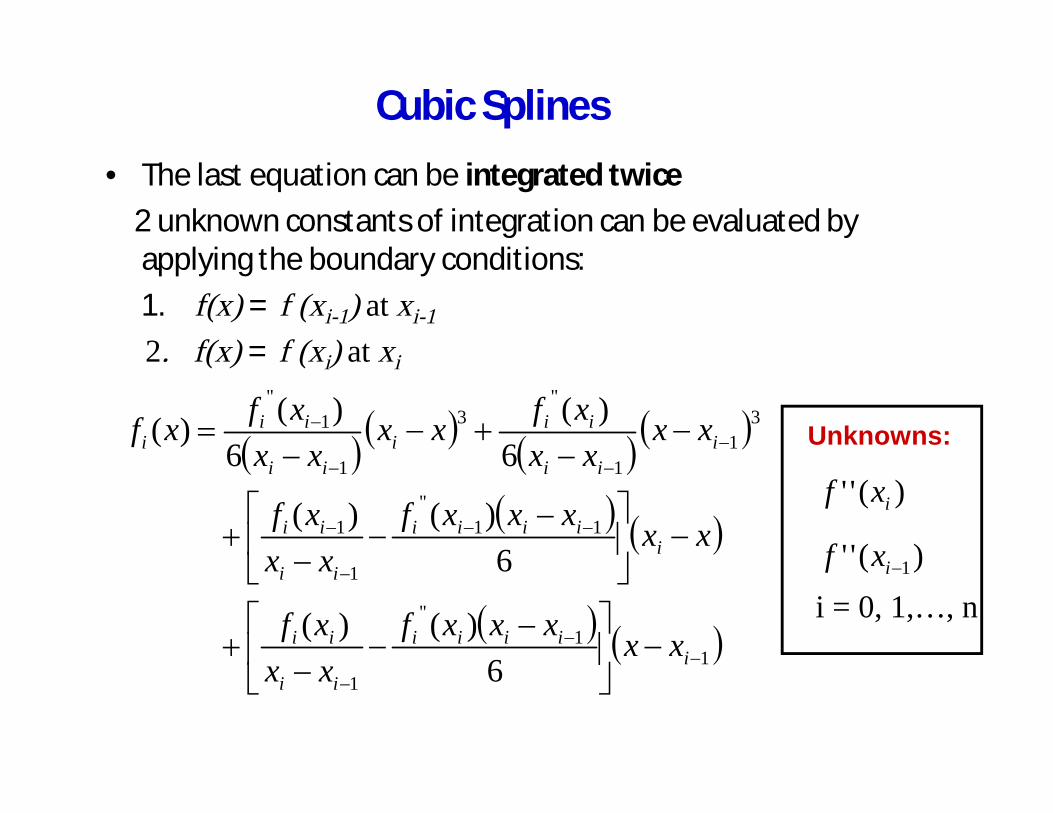
Cubic Splines• The last equation can be integrated twice
2 unknown constants of integration can be evaluated byapplying the boundary conditions:1. f(x) = f (xi-1) at xi-1
2. f(x) = f (xi) at xi
11
''
1
11''
1
1
31
1
''3
1
1''
6)()(
6)()(
6)(
6)()(
iiiii
ii
ii
iiiii
ii
ii
iii
iii
ii
iii
xxxxxfxxxf
xxxxxfxx
xf
xxxx
xfxxxx
xfxf
)('' ixf
Unknowns:
)('' 1ixfi = 0, 1,…, n
Cubic Splines
)()(6
)()(6)()(
)()(2)()(
11
11
1''
1
''111
''1
iiii
iiii
iii
iiiiii
xfxfxx
xfxfxx
xfxx
xfxxxfxx
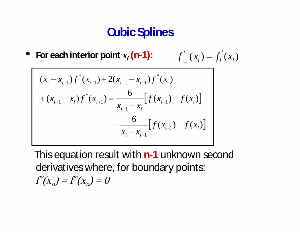
• For each interior point xi (n-1):
This equation result with n-1 unknown secondderivatives where, for boundary points:
(xo) = f (xn) = 0
)()( ''1 iii xfxf
i
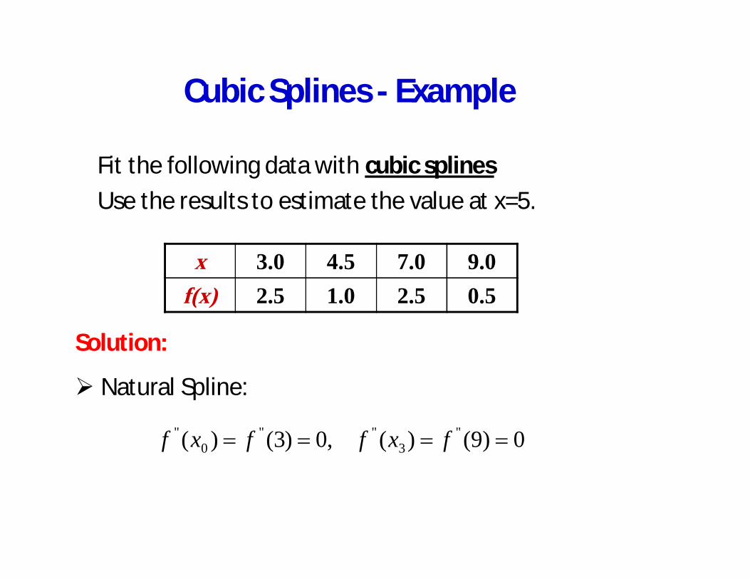
Cubic Splines - Example
Fit the following data with cubic splinesUse the results to estimate the value at x=5.
Solution:
Natural Spline:
x 3.0 4.5 7.0 9.0f(x) 2.5 1.0 2.5 0.5
0)9()(,0)3()( ''3
''''0
'' fxffxf
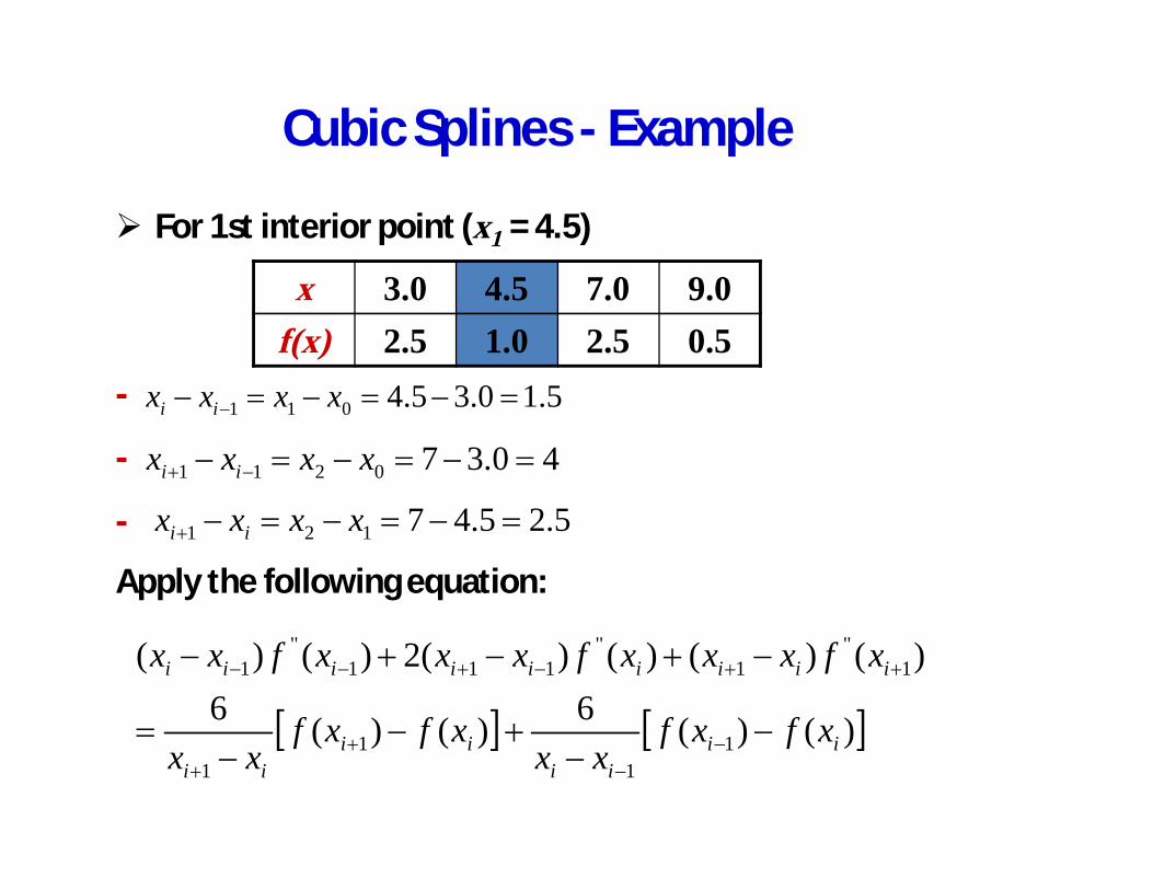
Cubic Splines - Example
For 1st interior point (x1 = 4.5)
-
-
-Apply the following equation:
)()(6)()(6)()()()(2)()(
11
11
1''
1''
111''
1
iiii
iiii
iiiiiiiii
xfxfxx
xfxfxx
xfxxxfxxxfxx
x 3.0 4.5 7.0 9.0f(x) 2.5 1.0 2.5 0.5
5.10.35.4011 xxxx ii
5.25.47121 xxxx ii
40.370211 xxxx ii
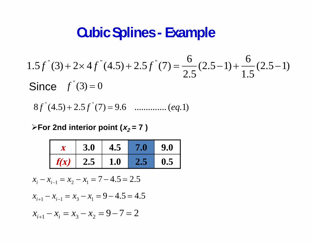
Cubic Splines - Example
)15.2(5.1
6)15.2(5.2
6)7(5.2)5.4(42)3(5.1 '''''' fff
0)3(''f
)1.(..............6.9)7(5.2)5.4(8 '''' eqff
x 3.0 4.5 7.0 9.0f(x) 2.5 1.0 2.5 0.5
Since
For 2nd interior point (x2 = 7 )
5.25.47121 xxxx ii
5.45.491311 xxxx ii
279231 xxxx ii
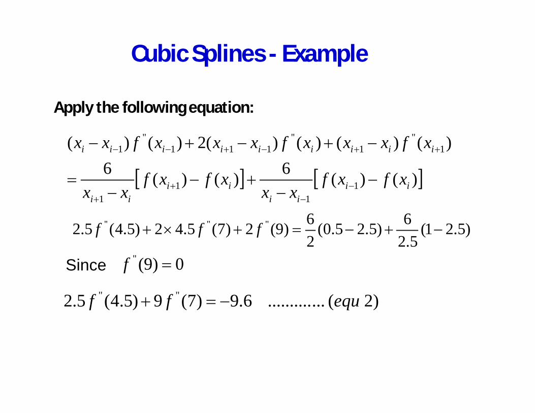
Cubic Splines - Example
Apply the following equation:
)()(6)()(6)()()()(2)()(
11
11
1''
1''
111''
1
iiii
iiii
iiiiiiiii
xfxfxx
xfxfxx
xfxxxfxxxfxx
)5.21(5.2
6)5.25.0(26)9(2)7(5.42)5.4(5.2 '''''' fff
Since 0)9(''f
)2(.............6.9)7(9)5.4(5.2 '''' equff
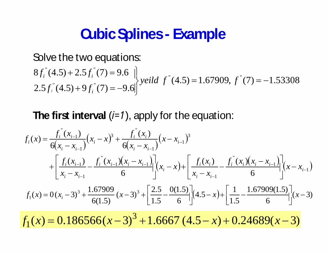
Cubic Splines - ExampleSolve the two equations:
The first interval (i=1), apply for the equation:
53308.1)7(,67909.1)5.4(6.9)7(9)5.4(5.2
6.9)7(5.2)5.4(8 ''''''''
''''
ffyeildffff
i
ii
i
11
''
1
11''
1
1
31
1
''3
1
1''
6)()(
6)()(
6)(
6)()(
iiiii
ii
iii
iiii
ii
ii
iii
iii
ii
iii
xxxxxfxxxfxxxxxf
xxxf
xxxx
xfxxxx
xfxf
)3(24689.0)5.4(6667.1)3(186566.0)( 31 xxxxf
)3(6
)5.1(67909.15.1
15.46
)5.1(05.15.2)3(
)5.1(667909.1)3(0)( 33
1 xxxxxf i
Cubic Splines - Example
)5.4(6
)5.2(53308.15.25.2
76
)5.2(67909.15.2
1)5.4()5.2(6
53308.1)7()5.2(6
67909.1)( 332
x
xxxxf
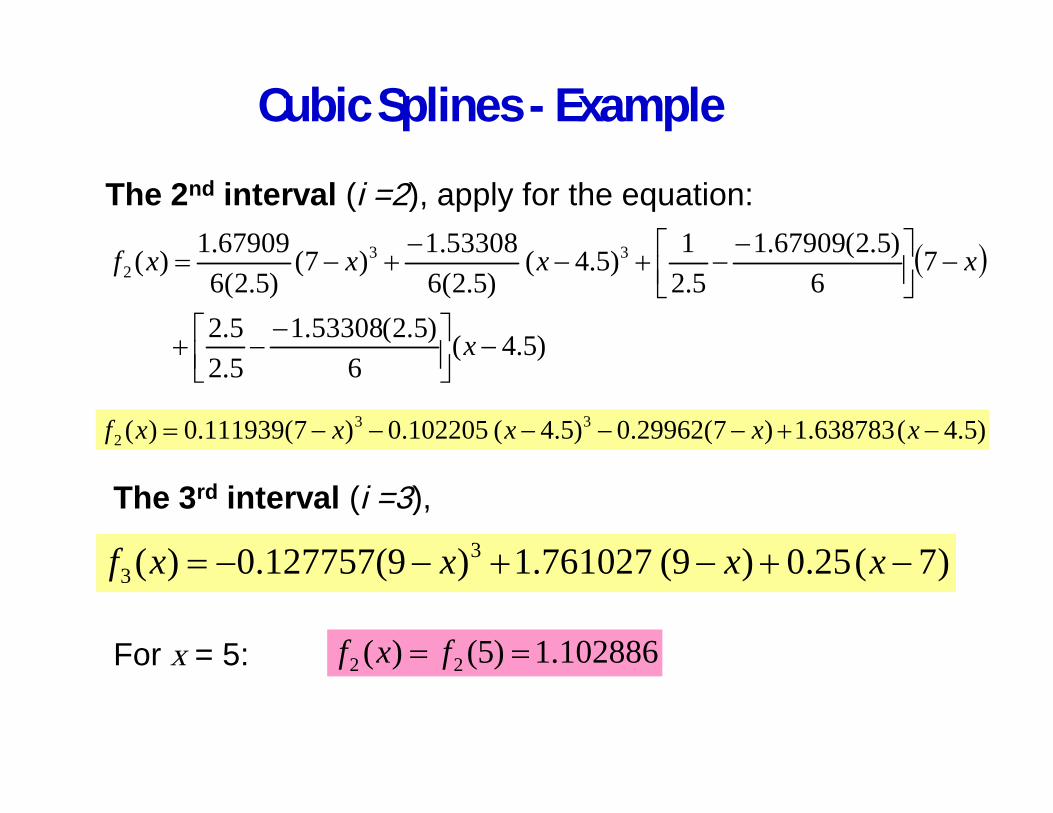
)5.4(638783.1)7(29962.0)5.4(102205.0)7(111939.0)( 332 xxxxxf
)7(25.0)9(761027.1)9(127757.0)( 33 xxxxf
102886.1)5()( 22 fxf
The 2nd interval (i =2), apply for the equation:
The 3rd interval (i =3),
For x = 5: