8-1

Regression with Panel Data (SW Ch. 10)

A panel dataset contains observations on multiple entities (individuals), where each entity is observed at two or more points in time.

Examples: • Data on 420 California school districts in 1999 and

again in 2000, for 840 observations total. • Data on 50 U.S. states, each state is observed in 3

years, for a total of 150 observations. • Data on 1000 individuals, in four different months,

for 4000 observations total.

8-2

Notation for panel data A double subscript distinguishes entities (states) and time periods (years)

i = entity (state), n = number of entities,

so i = 1,…,n t = time period (year), T = number of time periods

so t =1,…,T Data: Suppose we have 1 regressor. The data are:

(Xit, Yit), i = 1,…,n, t = 1,…,T

8-3

Panel data notation, ctd. Panel data with k regressors:

(X1it, X2it,…,Xkit, Yit), i = 1,…,n, t = 1,…,T

n = number of entities (states) T = number of time periods (years) Some jargon…

• Another term for panel data is longitudinal data • balanced panel: no missing observations • unbalanced panel: some entities (states) are not

observed for some time periods (years)

8-4

Why are panel data useful? With panel data we can control for factors that:

• Vary across entities (states) but do not vary over time • Could cause omitted variable bias if they are omitted • are unobserved or unmeasured – and therefore cannot

be included in the regression using multiple regression Here’s the key idea:

If an omitted variable does not change over time, then any changes in Y over time cannot be caused by the omitted variable.

8-5

Example of a panel data set: Traffic deaths and alcohol taxes

Observational unit: a year in a U.S. state

• 48 U.S. states, so n = of entities = 48 • 7 years (1982,…, 1988), so T = # of time periods = 7 • Balanced panel, so total # observations = 7×48 = 336

Variables: • Traffic fatality rate (# traffic deaths in that state in

that year, per 10,000 state residents) • Tax on a case of beer • Other (legal driving age, drunk driving laws, etc.)

8-6

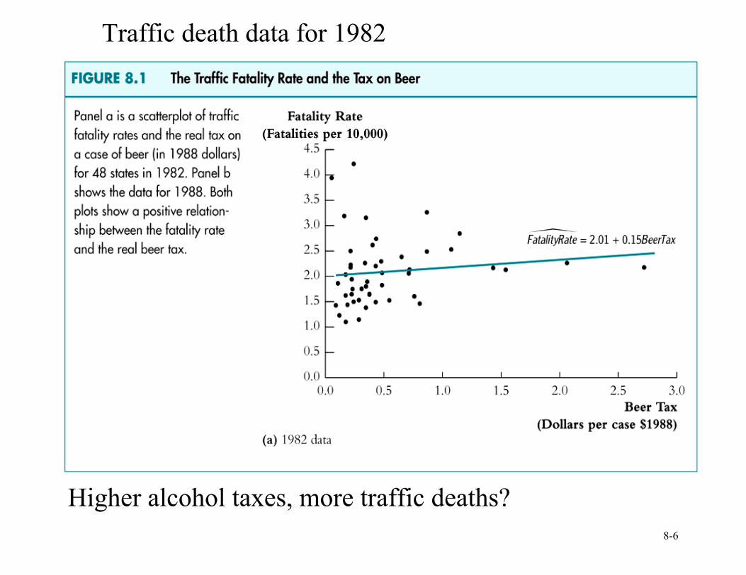
Traffic death data for 1982

Higher alcohol taxes, more traffic deaths?

8-7

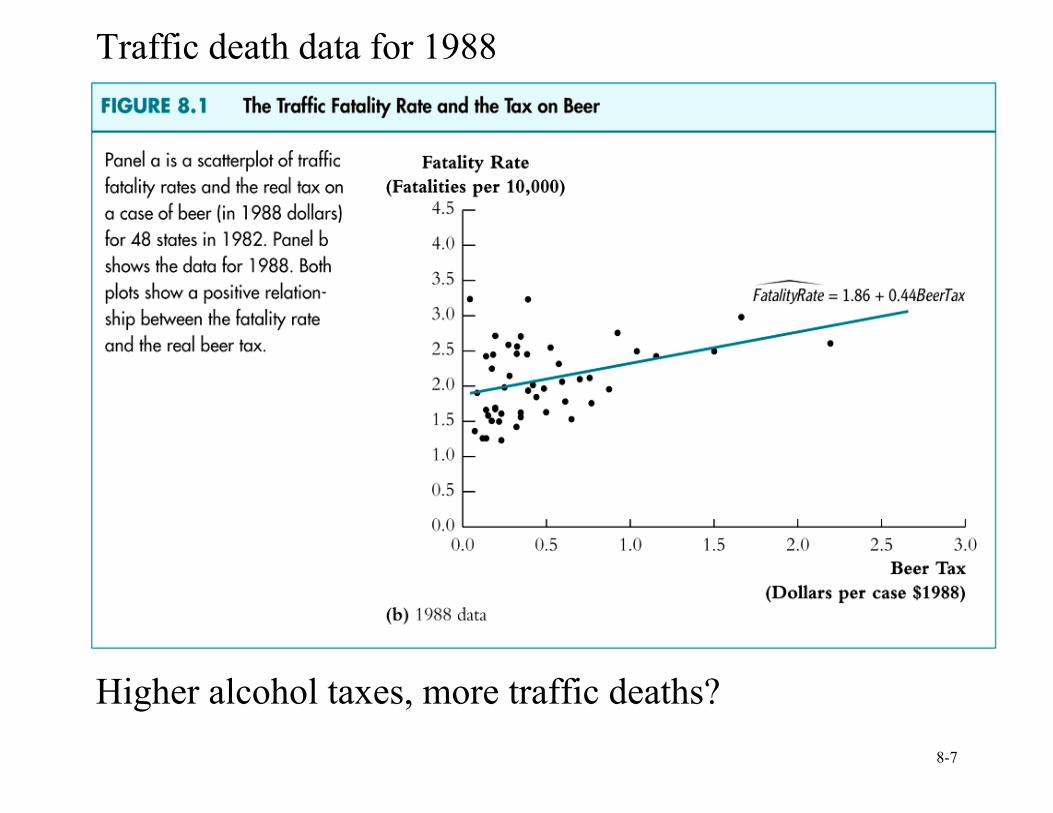
Traffic death data for 1988

Higher alcohol taxes, more traffic deaths?

8-8

Why might there be more traffic deaths in states that have higher alcohol taxes? Other factors that determine traffic fatality rate:

• Quality (age) of automobiles • Quality of roads • “Culture” around drinking and driving • Density of cars on the road

8-9

These omitted factors could cause omitted variable bias. Example #1: traffic density. Suppose:

(i) High traffic density means more traffic deaths (ii) (Western) states with lower traffic density have

lower alcohol taxes • Then the two conditions for omitted variable bias are

satisfied. Specifically, “high taxes” could reflect “high traffic density” (so the OLS coefficient would be biased positively – high taxes, more deaths)

• Panel data lets us eliminate omitted variable bias when the omitted variables are constant over time within a given state.

8-10

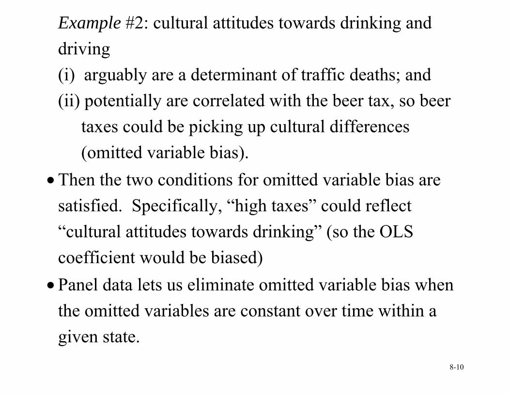
Example #2: cultural attitudes towards drinking and driving (i) arguably are a determinant of traffic deaths; and (ii) potentially are correlated with the beer tax, so beer

taxes could be picking up cultural differences (omitted variable bias).

• Then the two conditions for omitted variable bias are satisfied. Specifically, “high taxes” could reflect “cultural attitudes towards drinking” (so the OLS coefficient would be biased)

• Panel data lets us eliminate omitted variable bias when the omitted variables are constant over time within a given state.

8-11

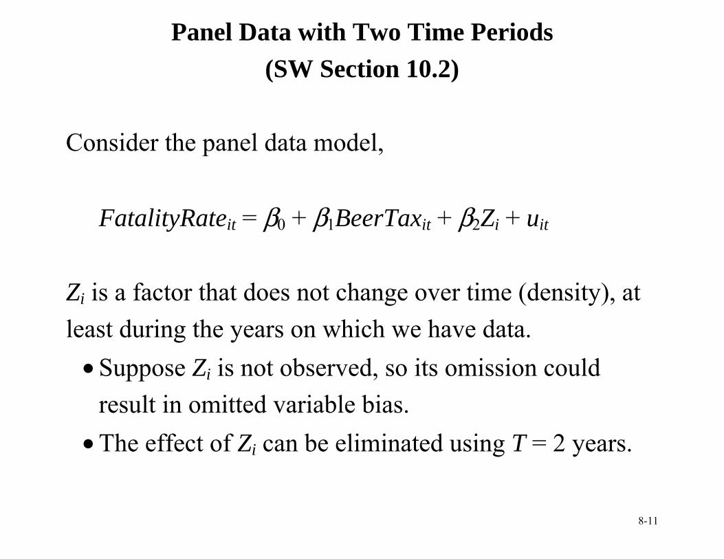
Panel Data with Two Time Periods (SW Section 10.2)

Consider the panel data model,

FatalityRateit = β0 + β1BeerTaxit + β2Zi + uit Zi is a factor that does not change over time (density), at least during the years on which we have data.

• Suppose Zi is not observed, so its omission could result in omitted variable bias.

• The effect of Zi can be eliminated using T = 2 years.

8-12

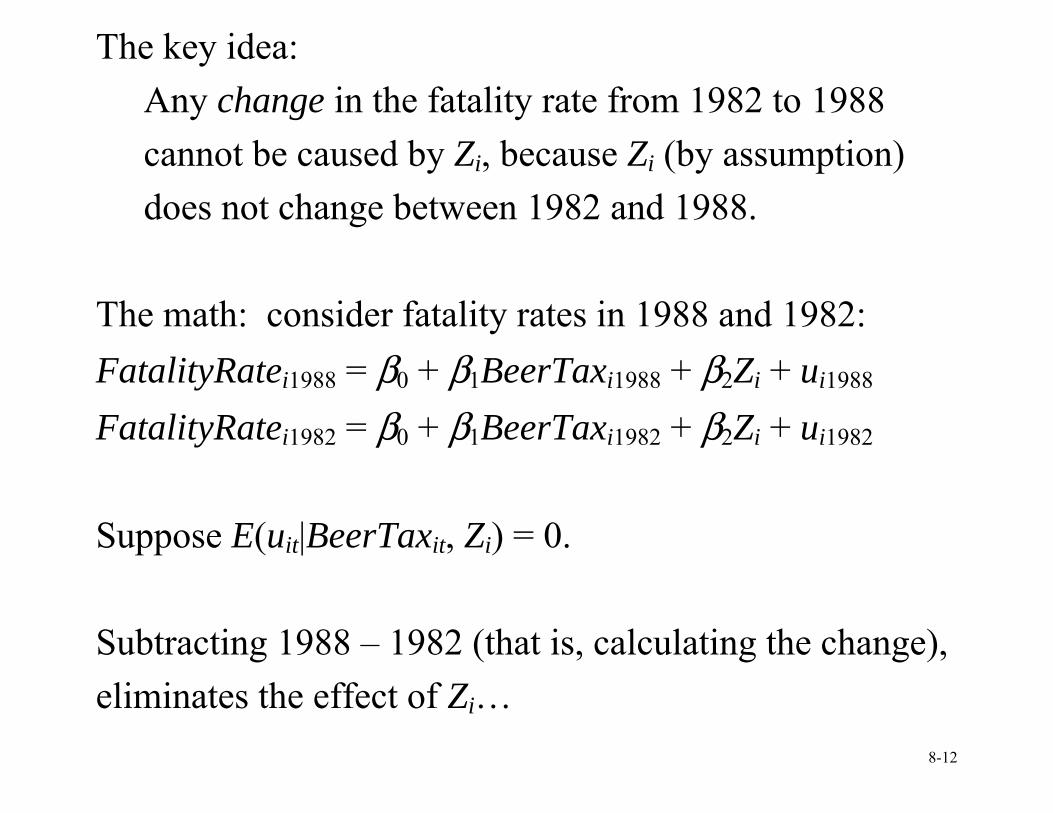
The key idea: Any change in the fatality rate from 1982 to 1988 cannot be caused by Zi, because Zi (by assumption) does not change between 1982 and 1988.

The math: consider fatality rates in 1988 and 1982: FatalityRatei1988 = β0 + β1BeerTaxi1988 + β2Zi + ui1988 FatalityRatei1982 = β0 + β1BeerTaxi1982 + β2Zi + ui1982 Suppose E(uit|BeerTaxit, Zi) = 0. Subtracting 1988 – 1982 (that is, calculating the change), eliminates the effect of Zi…

8-13

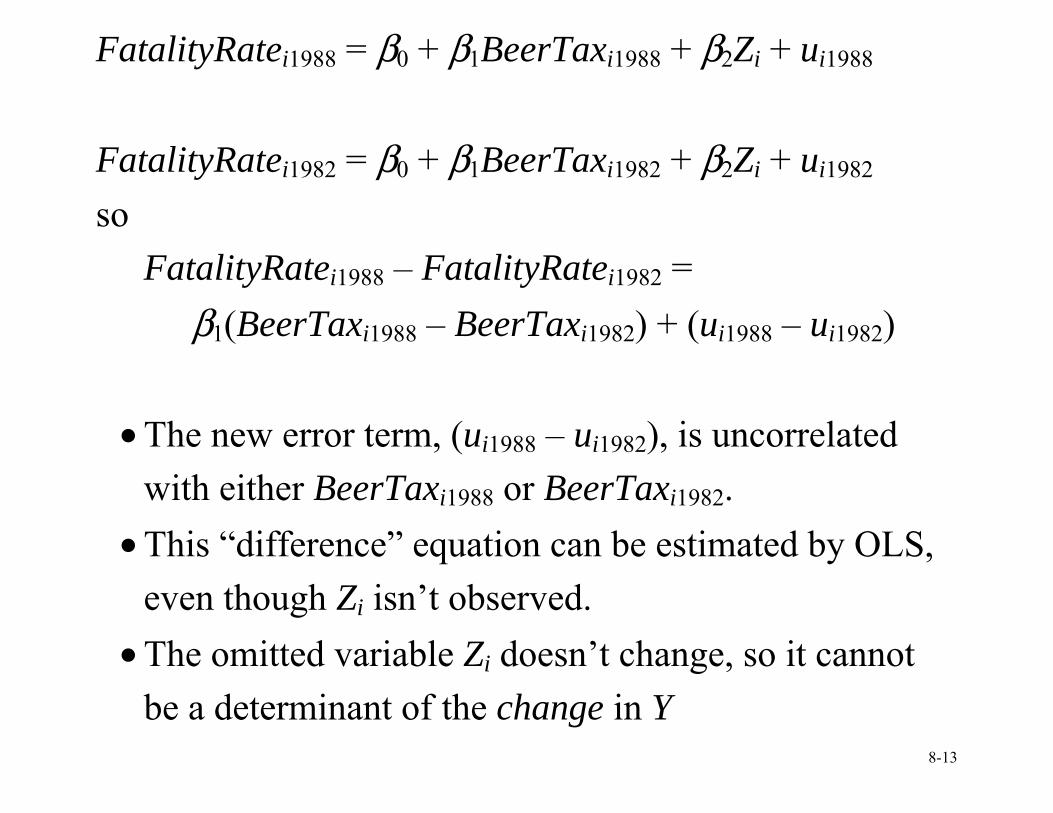
FatalityRatei1988 = β0 + β1BeerTaxi1988 + β2Zi + ui1988 FatalityRatei1982 = β0 + β1BeerTaxi1982 + β2Zi + ui1982 so

FatalityRatei1988 – FatalityRatei1982 = β1(BeerTaxi1988 – BeerTaxi1982) + (ui1988 – ui1982)

• The new error term, (ui1988 – ui1982), is uncorrelated with either BeerTaxi1988 or BeerTaxi1982.

• This “difference” equation can be estimated by OLS, even though Zi isn’t observed.

• The omitted variable Zi doesn’t change, so it cannot be a determinant of the change in Y

8-14

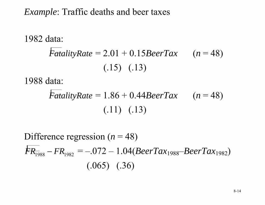
Example: Traffic deaths and beer taxes 1982 data:

FatalityRate = 2.01 + 0.15BeerTax (n = 48)

(.15) (.13) 1988 data:

FatalityRate = 1.86 + 0.44BeerTax (n = 48)

(.11) (.13) Difference regression (n = 48)

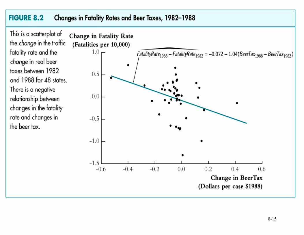
1988 1982FR FR− = –.072 – 1.04(BeerTax1988–BeerTax1982) (.065) (.36)

8-15

8-16

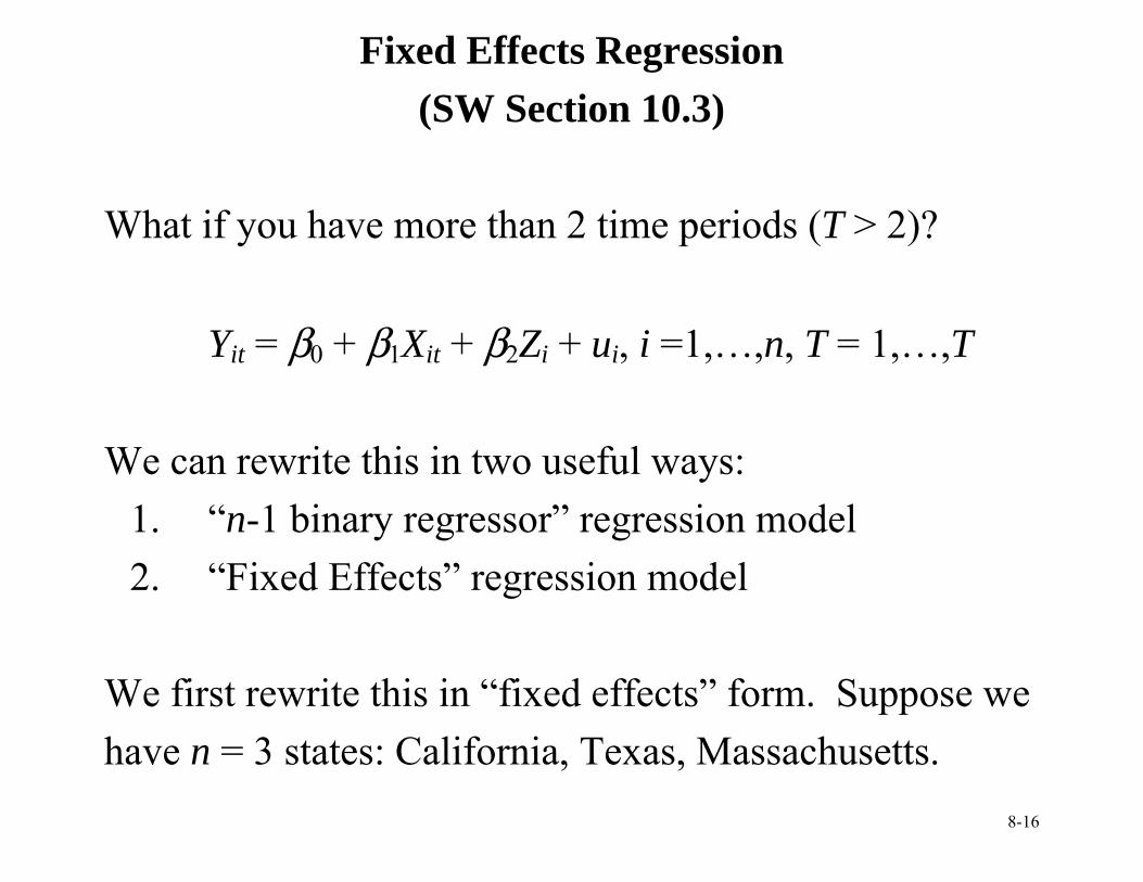
Fixed Effects Regression (SW Section 10.3)

What if you have more than 2 time periods (T > 2)?

Yit = β0 + β1Xit + β2Zi + ui, i =1,…,n, T = 1,…,T We can rewrite this in two useful ways:

1. “n-1 binary regressor” regression model 2. “Fixed Effects” regression model

We first rewrite this in “fixed effects” form. Suppose we have n = 3 states: California, Texas, Massachusetts.

8-17

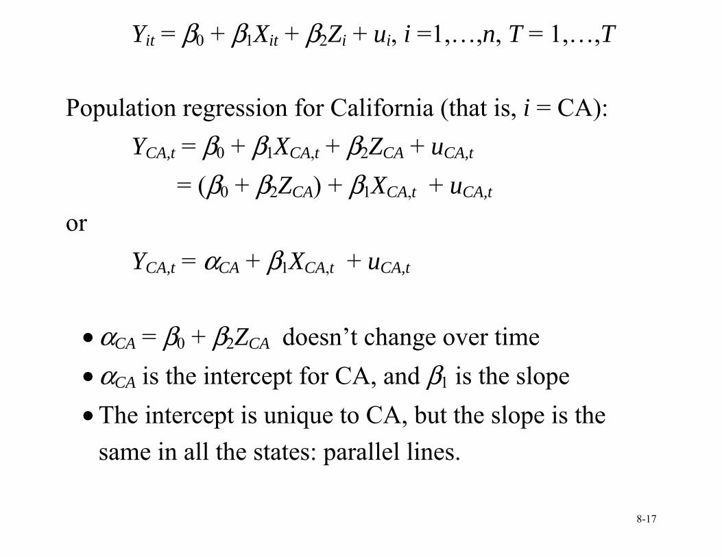
Yit = β0 + β1Xit + β2Zi + ui, i =1,…,n, T = 1,…,T Population regression for California (that is, i = CA):

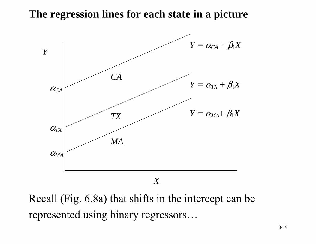
YCA,t = β0 + β1XCA,t + β2ZCA + uCA,t = (β0 + β2ZCA) + β1XCA,t + uCA,t or YCA,t = αCA + β1XCA,t + uCA,t

• αCA = β0 + β2ZCA doesn’t change over time • αCA is the intercept for CA, and β1 is the slope • The intercept is unique to CA, but the slope is the

same in all the states: parallel lines.

8-18

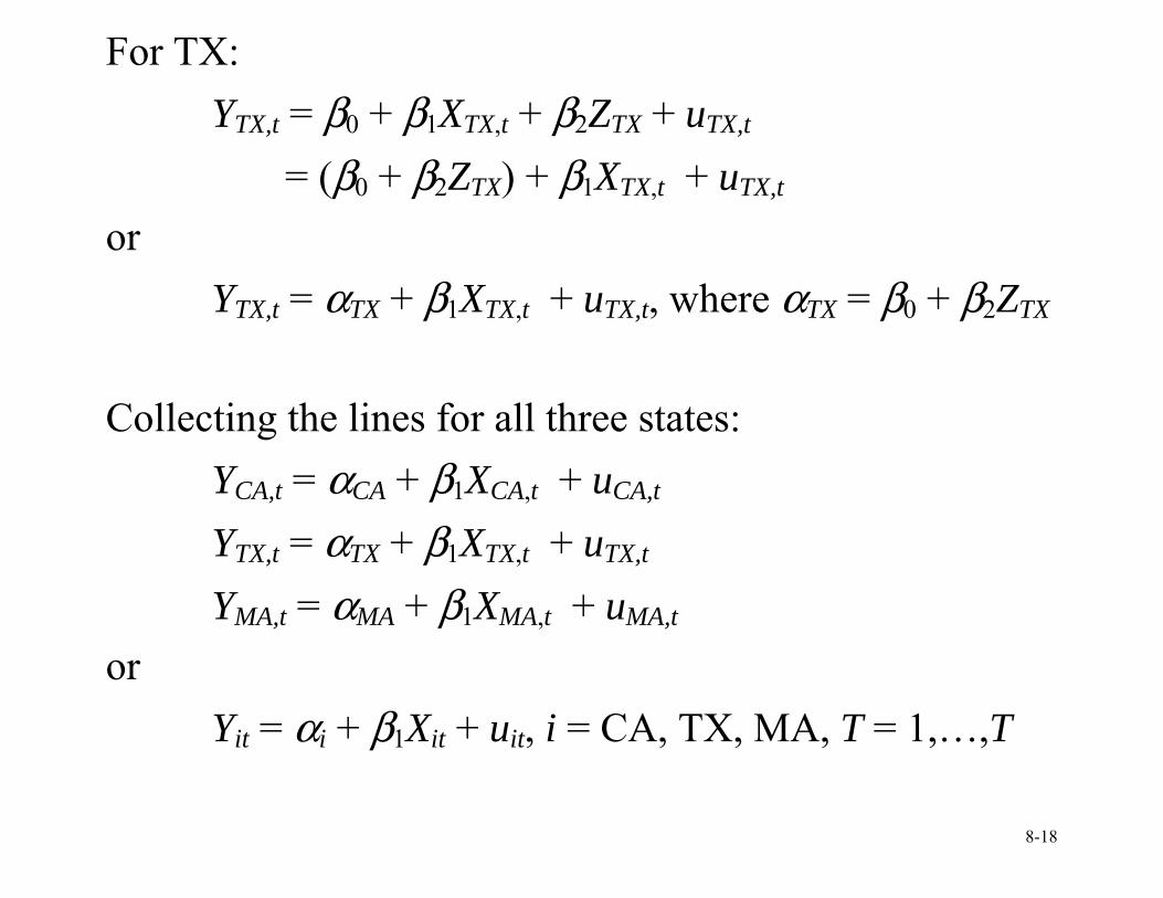
For TX: YTX,t = β0 + β1XTX,t + β2ZTX + uTX,t

= (β0 + β2ZTX) + β1XTX,t + uTX,t or YTX,t = αTX + β1XTX,t + uTX,t, where αTX = β0 + β2ZTX Collecting the lines for all three states: YCA,t = αCA + β1XCA,t + uCA,t YTX,t = αTX + β1XTX,t + uTX,t

YMA,t = αMA + β1XMA,t + uMA,t or Yit = αi + β1Xit + uit, i = CA, TX, MA, T = 1,…,T

8-19

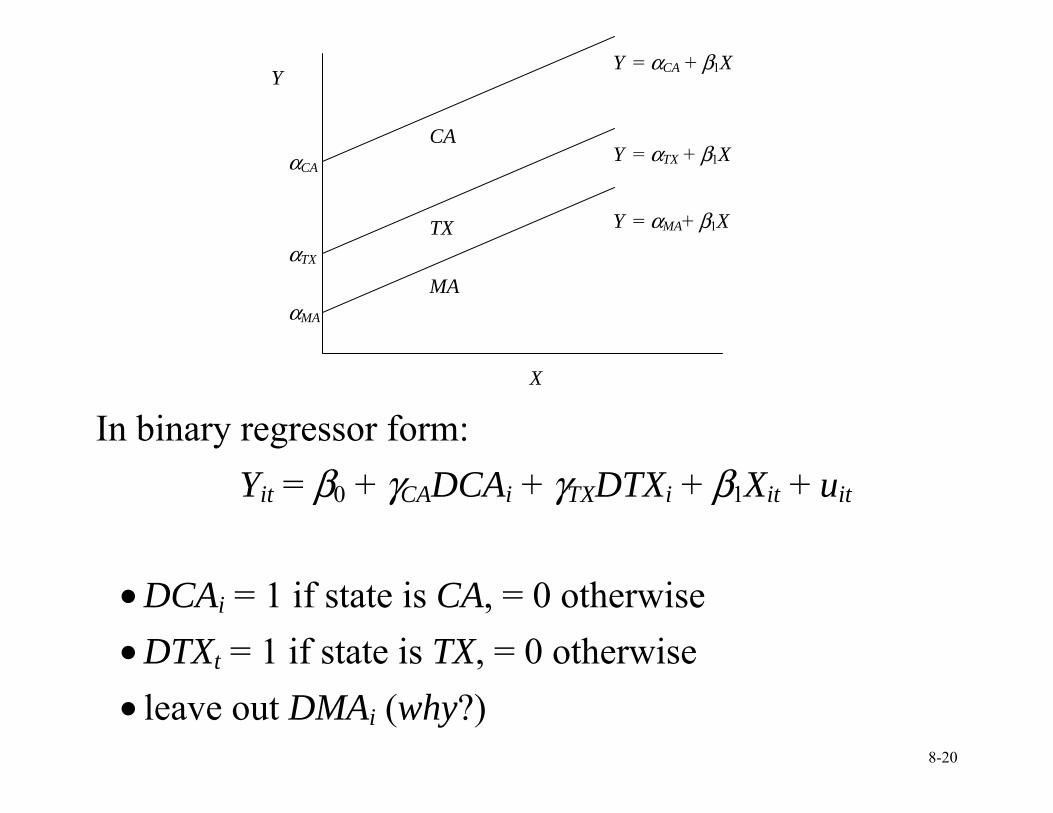
The regression lines for each state in a picture

Recall (Fig. 6.8a) that shifts in the intercept can be represented using binary regressors…

Y = αCA + β1X

Y = αTX + β1X

Y = αMA+ β1X

αMA

αTX

αCA

Y

X

MA

TX

CA

8-20

In binary regressor form:

Yit = β0 + γCADCAi + γTXDTXi + β1Xit + uit

• DCAi = 1 if state is CA, = 0 otherwise • DTXt = 1 if state is TX, = 0 otherwise • leave out DMAi (why?)

Y = αCA + β1X

Y = αTX + β1X

Y = αMA+ β1X

αMA

αTX

αCA

Y

X

MA

TX

CA

8-21

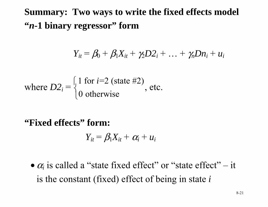
Summary: Two ways to write the fixed effects model “n-1 binary regressor” form

Yit = β0 + β1Xit + γ2D2i + … + γnDni + ui

where D2i = 1 for =2 (state #2)0 otherwise

i⎧⎨⎩

, etc.

“Fixed effects” form:

Yit = β1Xit + αi + ui • αi is called a “state fixed effect” or “state effect” – it

is the constant (fixed) effect of being in state i

8-22

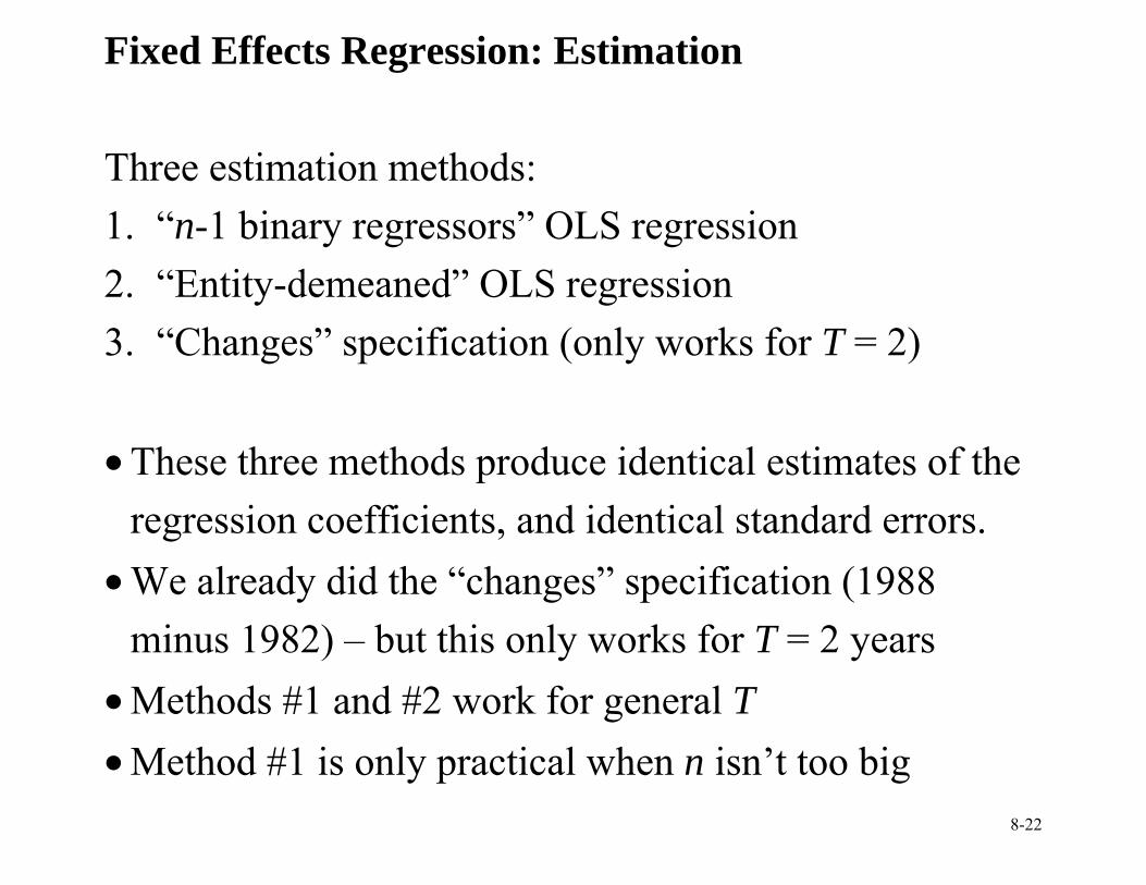
Fixed Effects Regression: Estimation Three estimation methods: 1. “n-1 binary regressors” OLS regression 2. “Entity-demeaned” OLS regression 3. “Changes” specification (only works for T = 2) • These three methods produce identical estimates of the

regression coefficients, and identical standard errors. • We already did the “changes” specification (1988

minus 1982) – but this only works for T = 2 years • Methods #1 and #2 work for general T • Method #1 is only practical when n isn’t too big

8-23

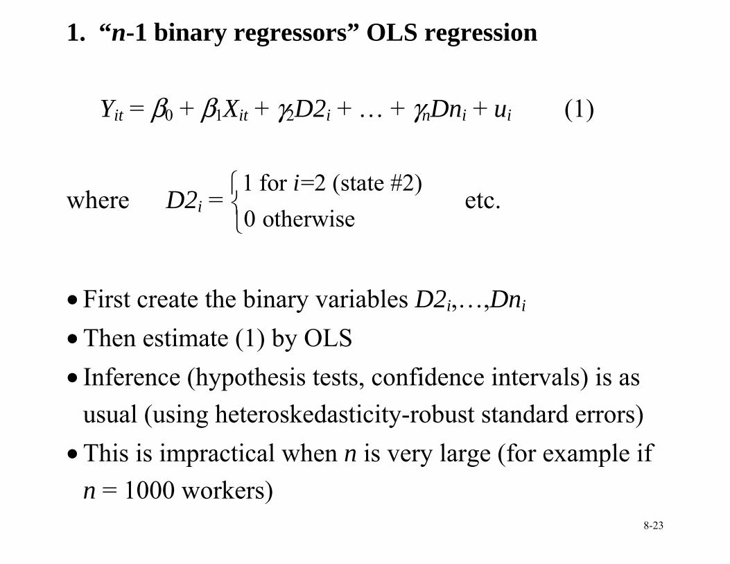
1. “n-1 binary regressors” OLS regression

Yit = β0 + β1Xit + γ2D2i + … + γnDni + ui (1)

where D2i = 1 for =2 (state #2)0 otherwise

i⎧⎨⎩

etc.

• First create the binary variables D2i,…,Dni • Then estimate (1) by OLS • Inference (hypothesis tests, confidence intervals) is as

usual (using heteroskedasticity-robust standard errors) • This is impractical when n is very large (for example if

n = 1000 workers)

8-24

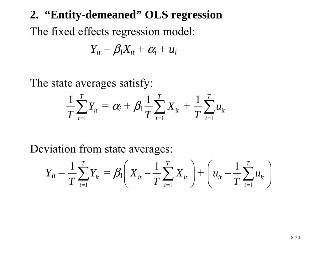
2. “Entity-demeaned” OLS regression The fixed effects regression model:

Yit = β1Xit + αi + ui The state averages satisfy:

1

1 T

itt

YT =∑ = αi + β1

1

1 T

itt

XT =∑ +

1

1 T

itt

uT =∑

Deviation from state averages:

Yit – 1

1 T

itt

YT =∑ = β1

1

1 T

it itt

X XT =

⎛ ⎞−⎜ ⎟⎝ ⎠

∑ + 1

1 T

it itt

u uT =

⎛ ⎞−⎜ ⎟⎝ ⎠

∑

8-25

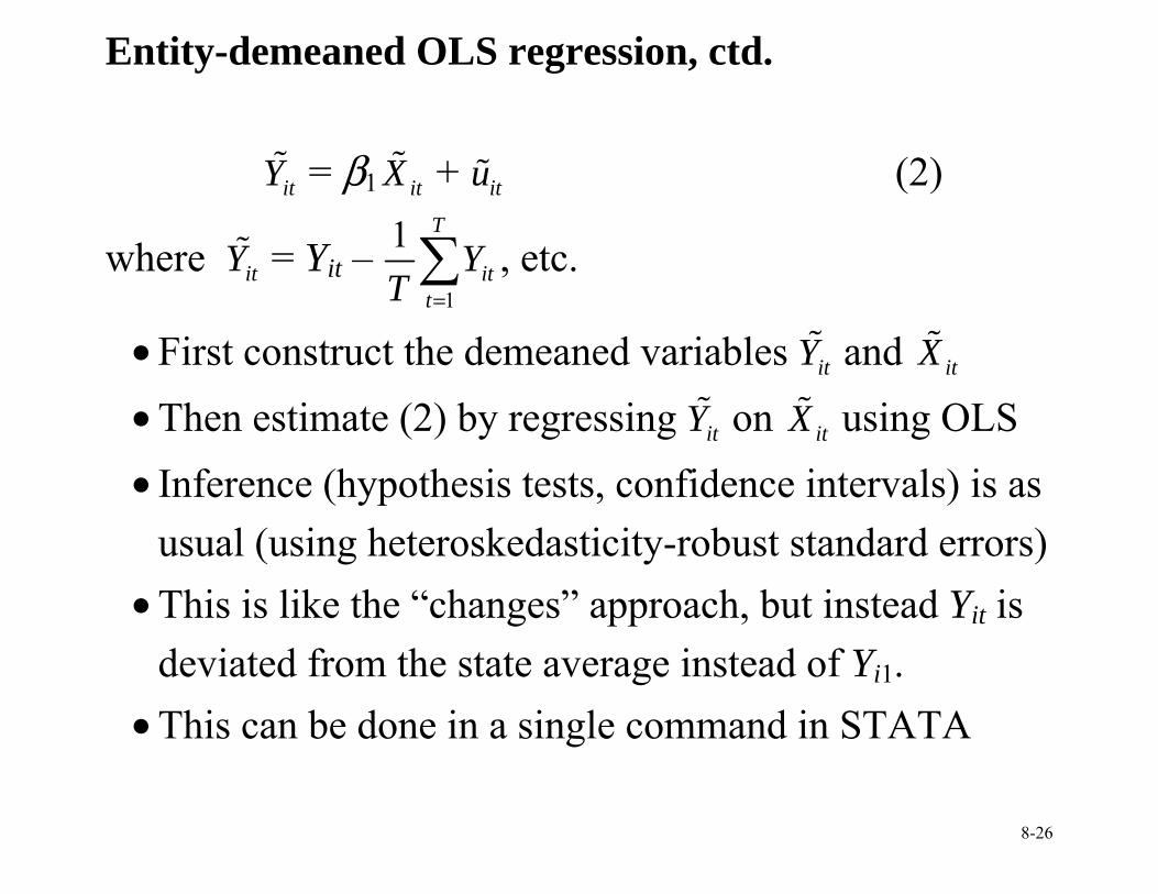
Entity-demeaned OLS regression, ctd.

Yit – 1

1 T

itt

YT =∑ = β1

1

1 T

it itt

X XT =

⎛ ⎞−⎜ ⎟⎝ ⎠

∑ + 1

1 T

it itt

u uT =

⎛ ⎞−⎜ ⎟⎝ ⎠

∑

or

itY% = β1 itX% + itu%

where itY% = Yit – 1

1 T

itt

YT =∑ and itX% = Xit –

1

1 T

itt

XT =∑

• For i=1 and t = 1982, itY% is the difference between the

fatality rate in Alabama in 1982, and its average value in Alabama averaged over all 7 years.

8-26

Entity-demeaned OLS regression, ctd.

itY% = β1 itX% + itu% (2)

where itY% = Yit – 1

1 T

itt

YT =∑ , etc.

• First construct the demeaned variables itY% and itX% • Then estimate (2) by regressing itY% on itX% using OLS • Inference (hypothesis tests, confidence intervals) is as

usual (using heteroskedasticity-robust standard errors) • This is like the “changes” approach, but instead Yit is

deviated from the state average instead of Yi1. • This can be done in a single command in STATA

8-27

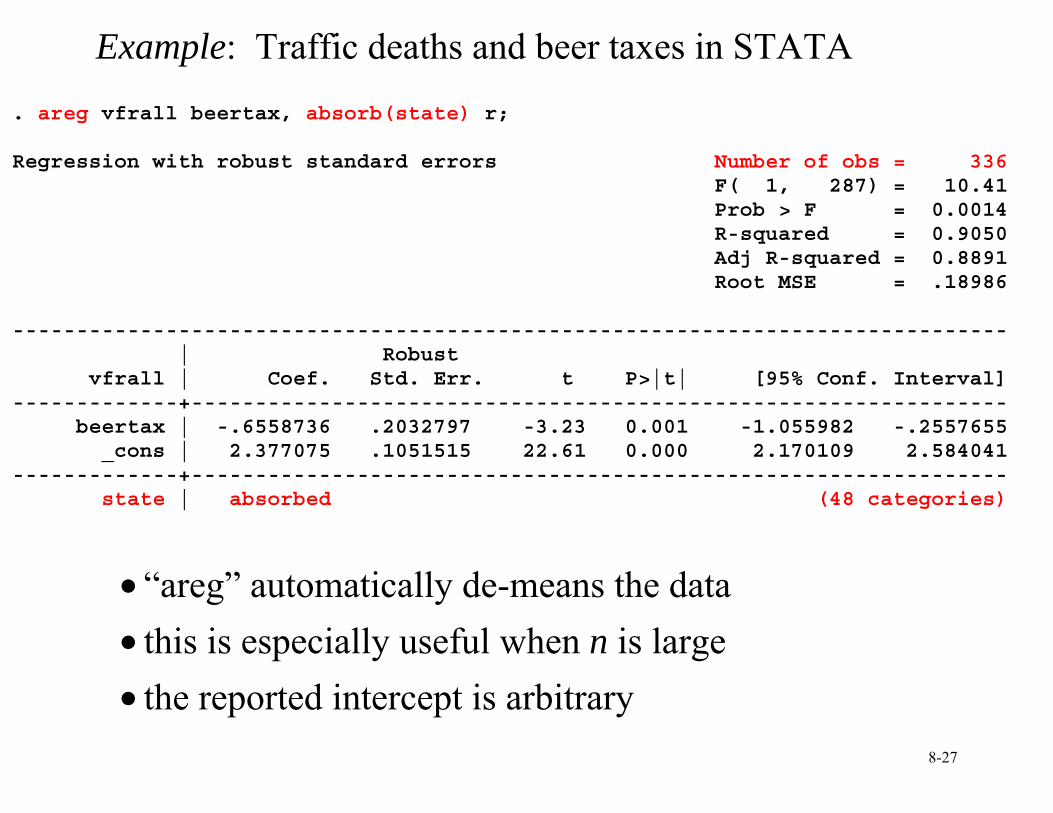
Example: Traffic deaths and beer taxes in STATA . areg vfrall beertax, absorb(state) r; Regression with robust standard errors Number of obs = 336 F( 1, 287) = 10.41 Prob > F = 0.0014 R-squared = 0.9050 Adj R-squared = 0.8891 Root MSE = .18986 ------------------------------------------------------------------------------ | Robust vfrall | Coef. Std. Err. t P>|t| [95% Conf. Interval] -------------+---------------------------------------------------------------- beertax | -.6558736 .2032797 -3.23 0.001 -1.055982 -.2557655 _cons | 2.377075 .1051515 22.61 0.000 2.170109 2.584041 -------------+---------------------------------------------------------------- state | absorbed (48 categories)

• “areg” automatically de-means the data • this is especially useful when n is large • the reported intercept is arbitrary

8-28

Example, ctd. For n = 48, T = 7:

FatalityRate = –.66BeerTax + State fixed effects (.20)

• Should you report the intercept? • How many binary regressors would you include to

estimate this using the “binary regressor” method? • Compare slope, standard error to the estimate for the

1988 v. 1982 “changes” specification (T = 2, n = 48):

1988 1982FR FR− = –.072 – 1.04(BeerTax1988–BeerTax1982) (.065) (.36)

8-29

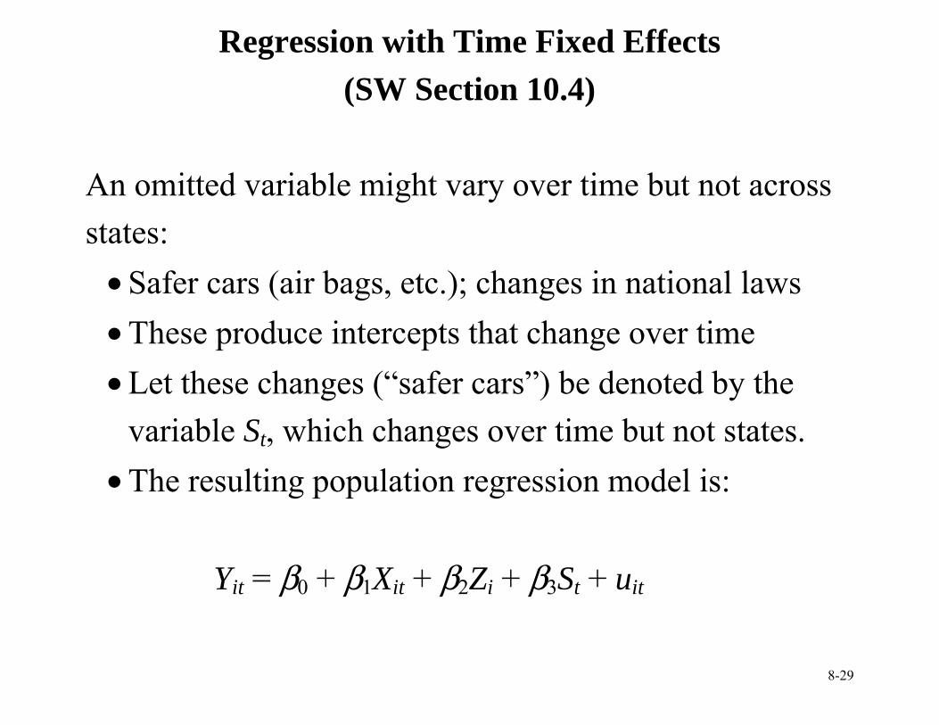
Regression with Time Fixed Effects (SW Section 10.4)

An omitted variable might vary over time but not across states:

• Safer cars (air bags, etc.); changes in national laws • These produce intercepts that change over time • Let these changes (“safer cars”) be denoted by the

variable St, which changes over time but not states. • The resulting population regression model is:

Yit = β0 + β1Xit + β2Zi + β3St + uit

8-30

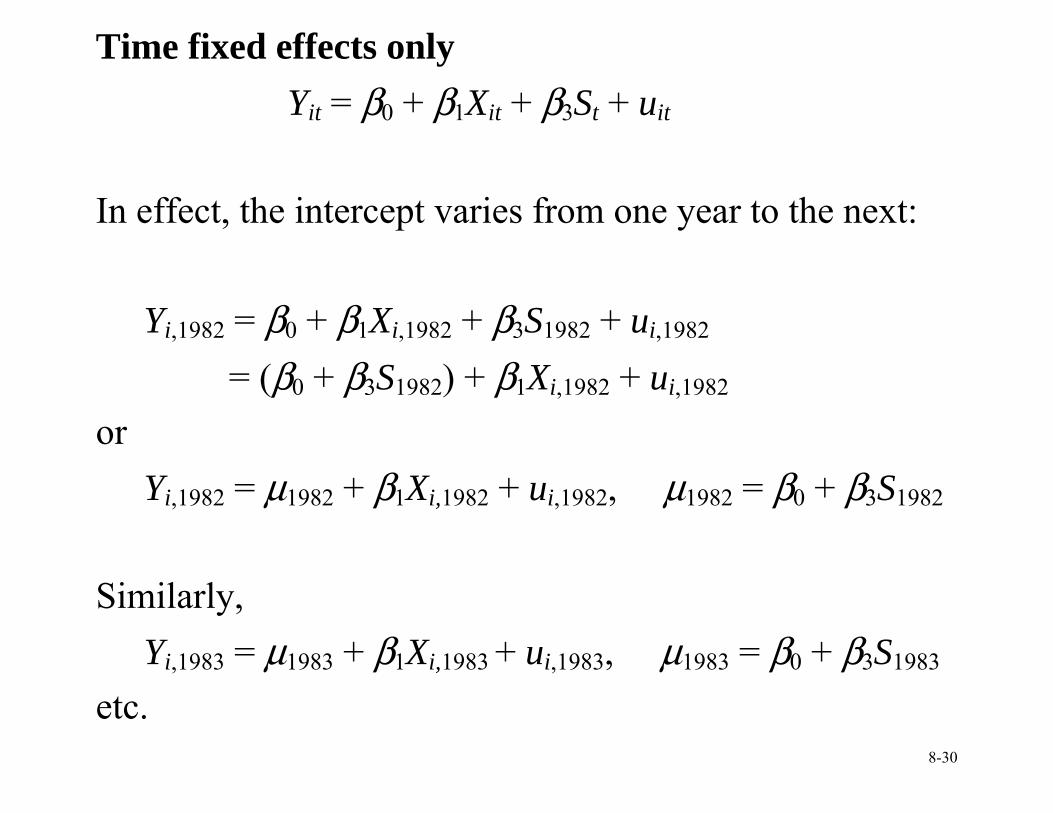
Time fixed effects only Yit = β0 + β1Xit + β3St + uit

In effect, the intercept varies from one year to the next:

Yi,1982 = β0 + β1Xi,1982 + β3S1982 + ui,1982

= (β0 + β3S1982) + β1Xi,1982 + ui,1982

or Yi,1982 = µ1982 + β1Xi,1982 + ui,1982, µ1982 = β0 + β3S1982

Similarly,

Yi,1983 = µ1983 + β1Xi,1983 + ui,1983, µ1983 = β0 + β3S1983 etc.

8-31

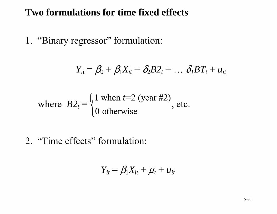
Two formulations for time fixed effects 1. “Binary regressor” formulation:

Yit = β0 + β1Xit + δ2B2t + … δTBTt + uit

where B2t = 1 when =2 (year #2)0 otherwise

t⎧⎨⎩

, etc.

2. “Time effects” formulation:

Yit = β1Xit + µt + uit

8-32

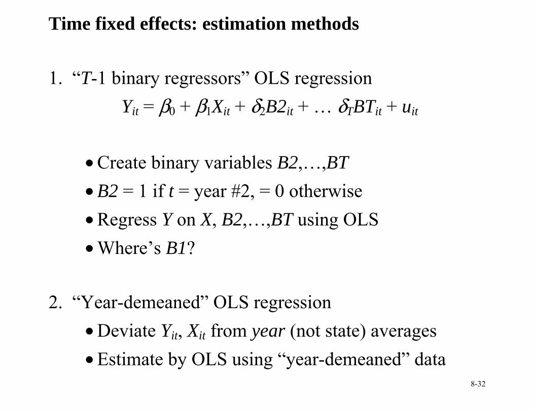
Time fixed effects: estimation methods 1. “T-1 binary regressors” OLS regression

Yit = β0 + β1Xit + δ2B2it + … δTBTit + uit • Create binary variables B2,…,BT • B2 = 1 if t = year #2, = 0 otherwise • Regress Y on X, B2,…,BT using OLS • Where’s B1?

2. “Year-demeaned” OLS regression

• Deviate Yit, Xit from year (not state) averages • Estimate by OLS using “year-demeaned” data

8-33

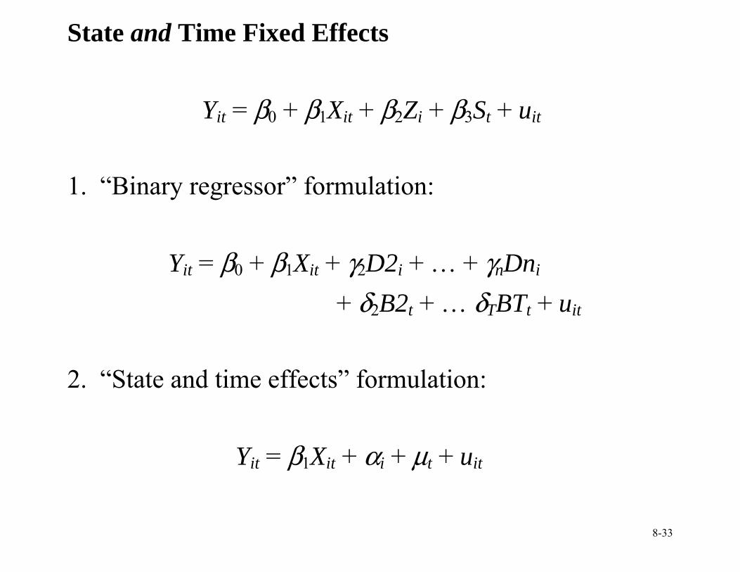
State and Time Fixed Effects

Yit = β0 + β1Xit + β2Zi + β3St + uit 1. “Binary regressor” formulation:

Yit = β0 + β1Xit + γ2D2i + … + γnDni + δ2B2t + … δTBTt + uit

2. “State and time effects” formulation:

Yit = β1Xit + αi + µt + uit

8-34

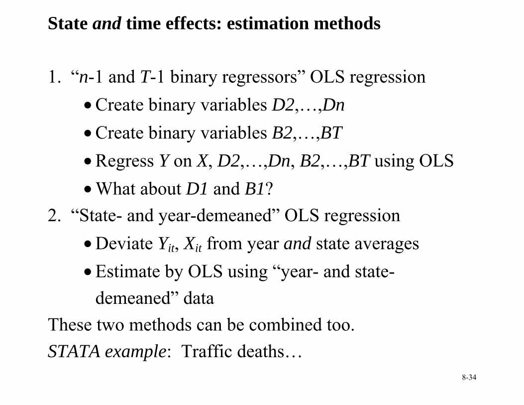
State and time effects: estimation methods 1. “n-1 and T-1 binary regressors” OLS regression

• Create binary variables D2,…,Dn • Create binary variables B2,…,BT • Regress Y on X, D2,…,Dn, B2,…,BT using OLS • What about D1 and B1?

2. “State- and year-demeaned” OLS regression • Deviate Yit, Xit from year and state averages • Estimate by OLS using “year- and state-

demeaned” data These two methods can be combined too. STATA example: Traffic deaths…

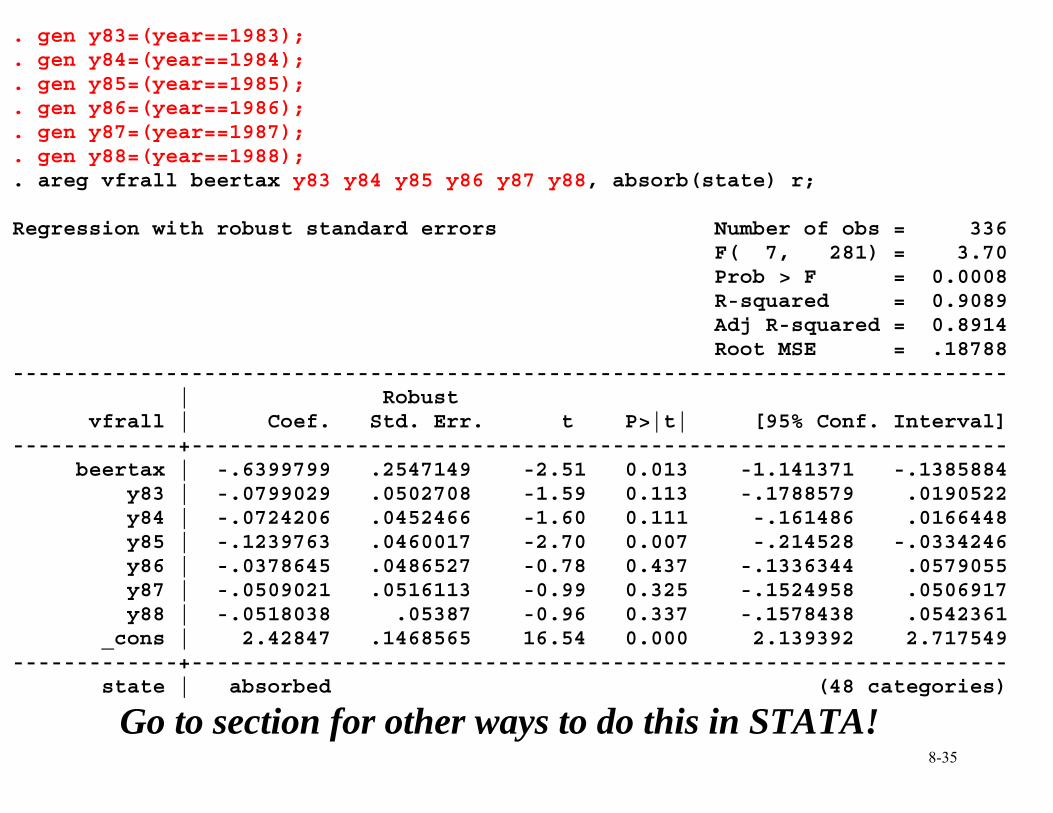
8-35

. gen y83=(year==1983);

. gen y84=(year==1984);

. gen y85=(year==1985);

. gen y86=(year==1986);

. gen y87=(year==1987);

. gen y88=(year==1988);

. areg vfrall beertax y83 y84 y85 y86 y87 y88, absorb(state) r; Regression with robust standard errors Number of obs = 336 F( 7, 281) = 3.70 Prob > F = 0.0008 R-squared = 0.9089 Adj R-squared = 0.8914 Root MSE = .18788 ------------------------------------------------------------------------------ | Robust vfrall | Coef. Std. Err. t P>|t| [95% Conf. Interval] -------------+---------------------------------------------------------------- beertax | -.6399799 .2547149 -2.51 0.013 -1.141371 -.1385884 y83 | -.0799029 .0502708 -1.59 0.113 -.1788579 .0190522 y84 | -.0724206 .0452466 -1.60 0.111 -.161486 .0166448 y85 | -.1239763 .0460017 -2.70 0.007 -.214528 -.0334246 y86 | -.0378645 .0486527 -0.78 0.437 -.1336344 .0579055 y87 | -.0509021 .0516113 -0.99 0.325 -.1524958 .0506917 y88 | -.0518038 .05387 -0.96 0.337 -.1578438 .0542361 _cons | 2.42847 .1468565 16.54 0.000 2.139392 2.717549 -------------+---------------------------------------------------------------- state | absorbed (48 categories)

Go to section for other ways to do this in STATA!

8-36

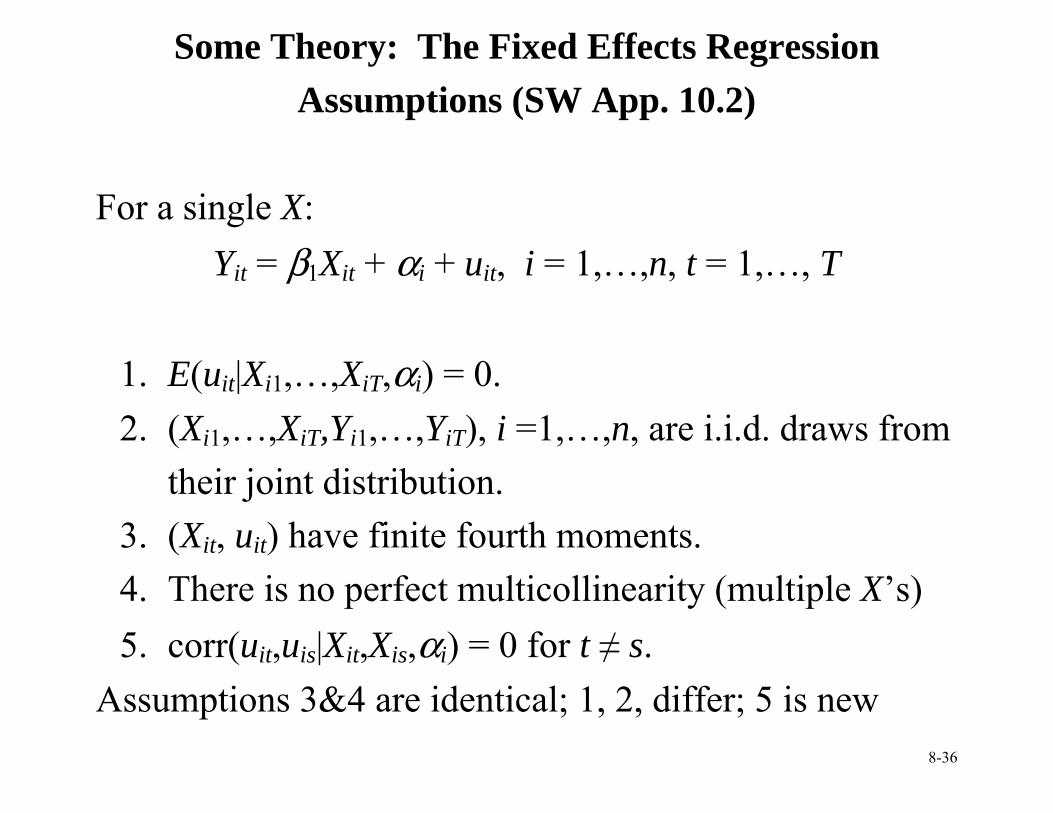
Some Theory: The Fixed Effects Regression Assumptions (SW App. 10.2)

For a single X:

Yit = β1Xit + αi + uit, i = 1,…,n, t = 1,…, T

1. E(uit|Xi1,…,XiT,αi) = 0. 2. (Xi1,…,XiT,Yi1,…,YiT), i =1,…,n, are i.i.d. draws from

their joint distribution. 3. (Xit, uit) have finite fourth moments. 4. There is no perfect multicollinearity (multiple X’s) 5. corr(uit,uis|Xit,Xis,αi) = 0 for t ≠ s.

Assumptions 3&4 are identical; 1, 2, differ; 5 is new

8-37

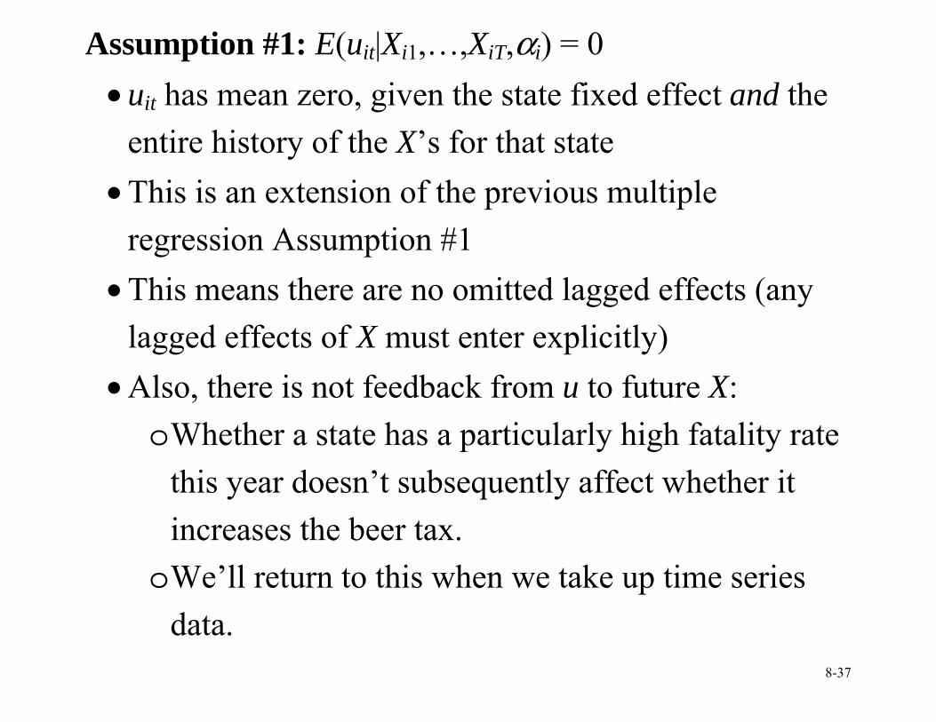
Assumption #1: E(uit|Xi1,…,XiT,αi) = 0 • uit has mean zero, given the state fixed effect and the

entire history of the X’s for that state • This is an extension of the previous multiple

regression Assumption #1 • This means there are no omitted lagged effects (any

lagged effects of X must enter explicitly) • Also, there is not feedback from u to future X:

o Whether a state has a particularly high fatality rate this year doesn’t subsequently affect whether it increases the beer tax.

o We’ll return to this when we take up time series data.

8-38

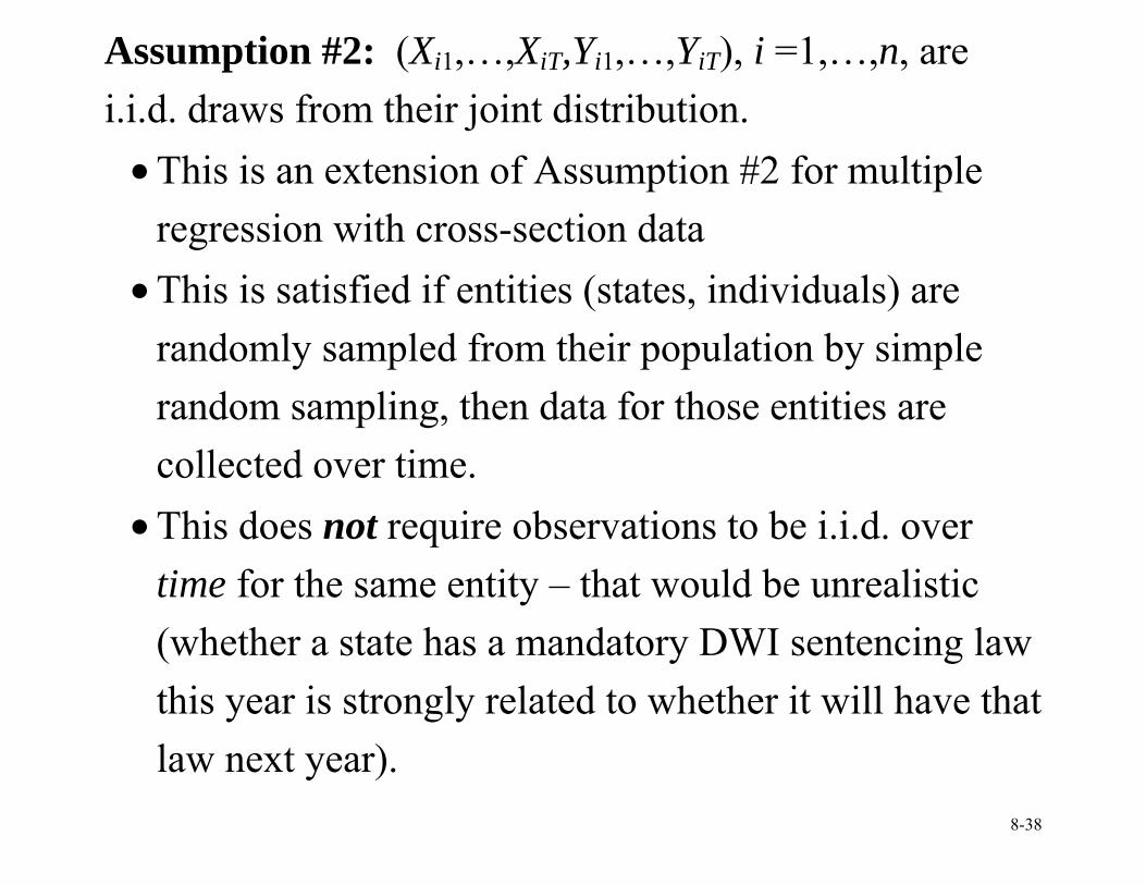
Assumption #2: (Xi1,…,XiT,Yi1,…,YiT), i =1,…,n, are i.i.d. draws from their joint distribution.

• This is an extension of Assumption #2 for multiple regression with cross-section data

• This is satisfied if entities (states, individuals) are randomly sampled from their population by simple random sampling, then data for those entities are collected over time.

• This does not require observations to be i.i.d. over time for the same entity – that would be unrealistic (whether a state has a mandatory DWI sentencing law this year is strongly related to whether it will have that law next year).

8-39

Assumption #5: corr(uit,uis|Xit,Xis,αi) = 0 for t ≠ s • This is new. • This says that (given X), the error terms are

uncorrelated over time within a state. • For example, uCA,1982 and uCA,1983 are uncorrelated • Is this plausible? What enters the error term?

o Especially snowy winter o Opening major new divided highway o Fluctuations in traffic density from local economic

conditions • Assumption #5 requires these omitted factors entering

uit to be uncorrelated over time, within a state.

8-40

What if Assumption #5 fails: corr(uit,uis|Xit,Xis,αi) ≠0? • A useful analogy is heteroskedasticity. • OLS panel data estimators of β1 are unbiased,

consistent • The OLS standard errors will be wrong – usually the

OLS standard errors understate the true uncertainty • Intuition: if uit is correlated over time, you don’t have

as much information (as much random variation) as you would were uit uncorrelated.

• This problem is solved by using “heteroskedasticity and autocorrelation-consistent standard errors” – we return to this when we focus on time series regression

8-41

Application: Drunk Driving Laws and Traffic Deaths (SW Section 10.5)

Some facts

• Approx. 40,000 traffic fatalities annually in the U.S. • 1/3 of traffic fatalities involve a drinking driver • 25% of drivers on the road between 1am and 3am

have been drinking (estimate) • A drunk driver is 13 times as likely to cause a fatal

crash as a non-drinking driver (estimate)

8-42

Drunk driving laws and traffic deaths, ctd. Public policy issues

• Drunk driving causes massive externalities (sober drivers are killed, etc. etc.) – there is ample justification for governmental intervention

• Are there any effective ways to reduce drunk driving? If so, what?

• What are effects of specific laws: o mandatory punishment o minimum legal drinking age o economic interventions (alcohol taxes)

8-43

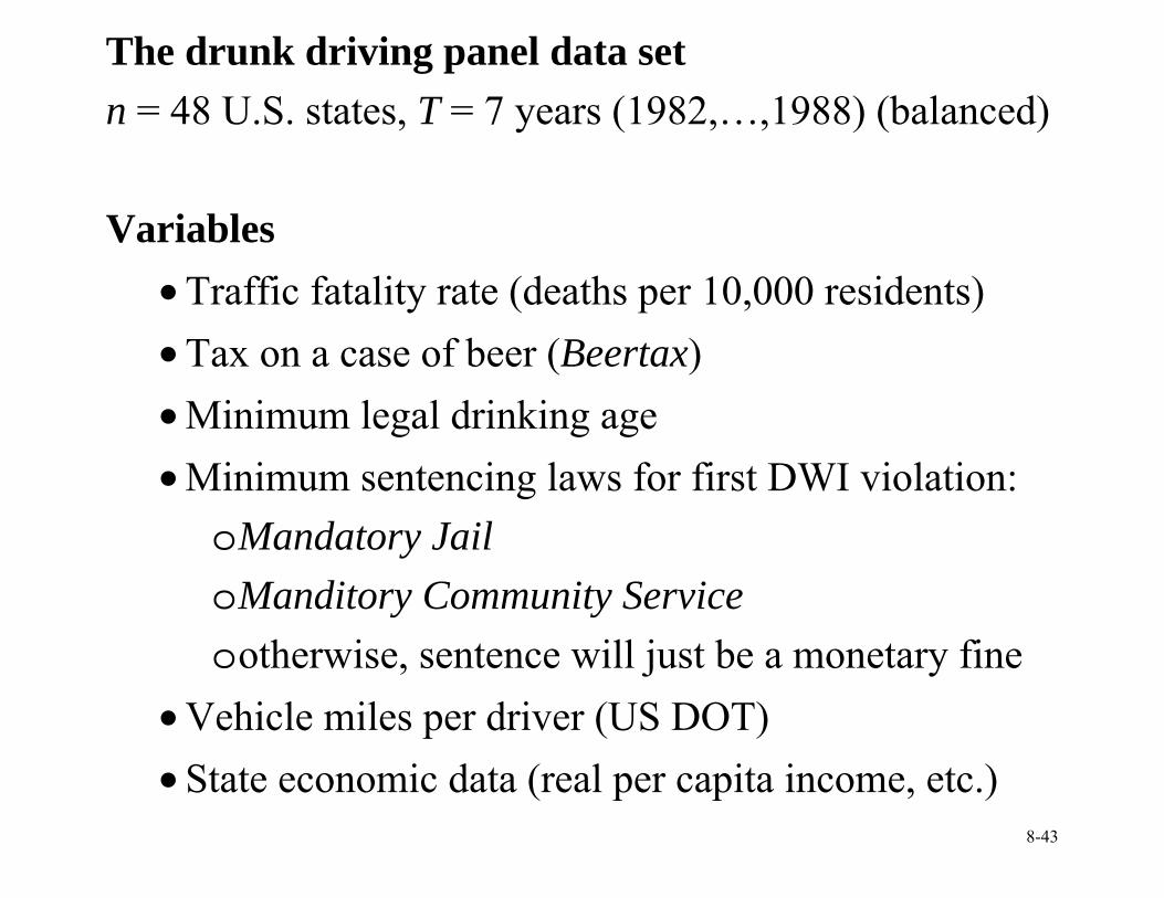
The drunk driving panel data set n = 48 U.S. states, T = 7 years (1982,…,1988) (balanced) Variables

• Traffic fatality rate (deaths per 10,000 residents) • Tax on a case of beer (Beertax) • Minimum legal drinking age • Minimum sentencing laws for first DWI violation:

o Mandatory Jail o Manditory Community Service o otherwise, sentence will just be a monetary fine

• Vehicle miles per driver (US DOT) • State economic data (real per capita income, etc.)

8-44

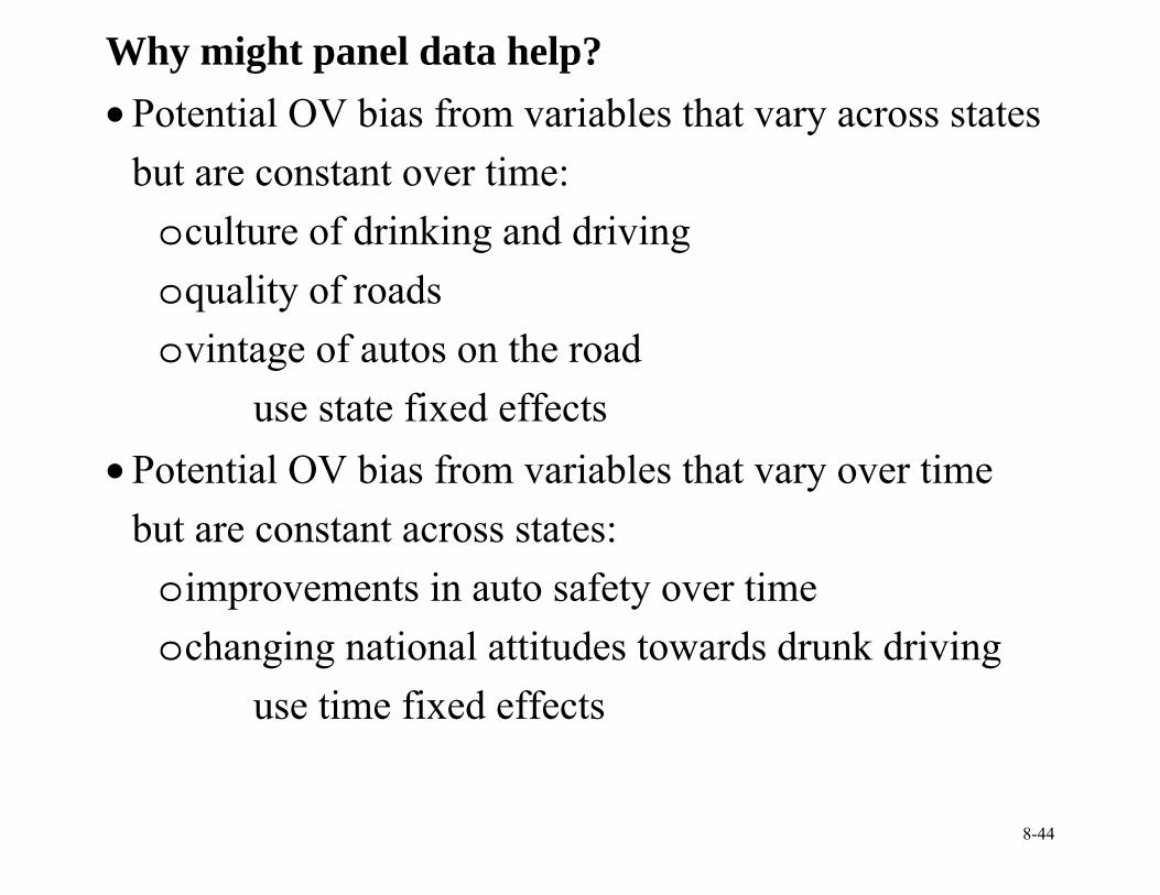
Why might panel data help? • Potential OV bias from variables that vary across states

but are constant over time: o culture of drinking and driving o quality of roads o vintage of autos on the road

� use state fixed effects • Potential OV bias from variables that vary over time

but are constant across states: o improvements in auto safety over time o changing national attitudes towards drunk driving

� use time fixed effects

8-45

8-46

8-47

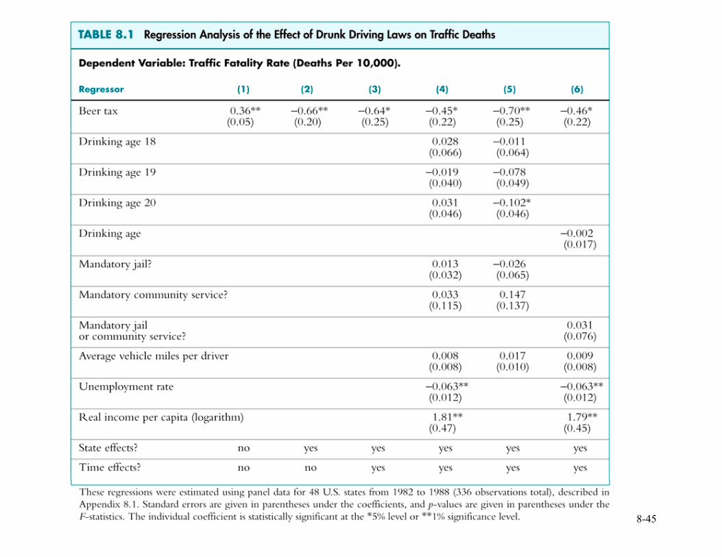
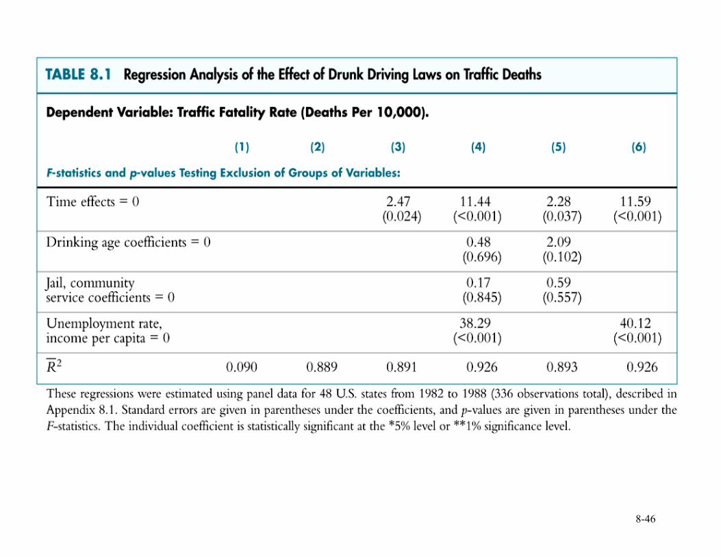
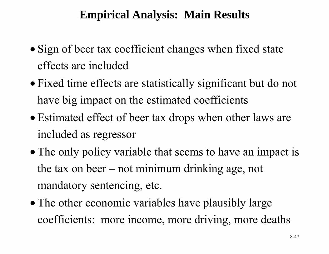
Empirical Analysis: Main Results • Sign of beer tax coefficient changes when fixed state

effects are included • Fixed time effects are statistically significant but do not

have big impact on the estimated coefficients • Estimated effect of beer tax drops when other laws are

included as regressor • The only policy variable that seems to have an impact is

the tax on beer – not minimum drinking age, not mandatory sentencing, etc.

• The other economic variables have plausibly large coefficients: more income, more driving, more deaths

8-48

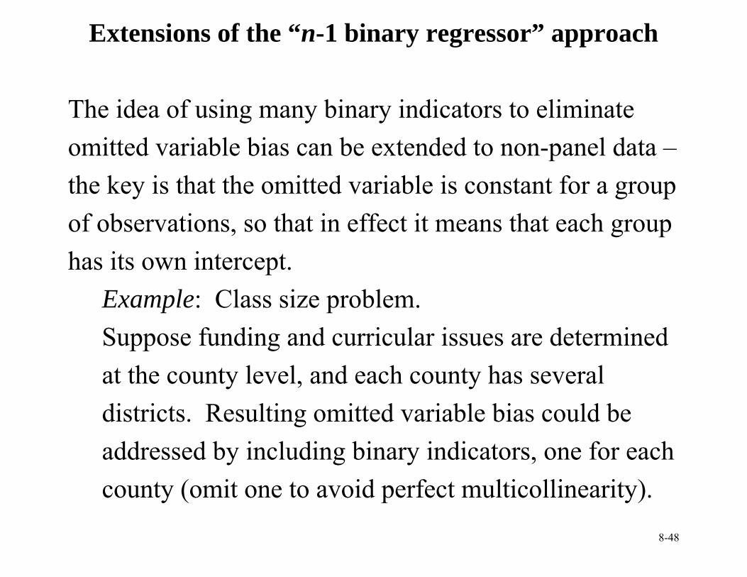
Extensions of the “n-1 binary regressor” approach The idea of using many binary indicators to eliminate omitted variable bias can be extended to non-panel data – the key is that the omitted variable is constant for a group of observations, so that in effect it means that each group has its own intercept.

Example: Class size problem. Suppose funding and curricular issues are determined at the county level, and each county has several districts. Resulting omitted variable bias could be addressed by including binary indicators, one for each county (omit one to avoid perfect multicollinearity).

8-49

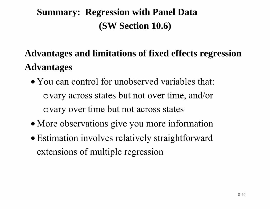
Summary: Regression with Panel Data (SW Section 10.6)

Advantages and limitations of fixed effects regression Advantages

• You can control for unobserved variables that: o vary across states but not over time, and/or o vary over time but not across states

• More observations give you more information • Estimation involves relatively straightforward

extensions of multiple regression

8-50

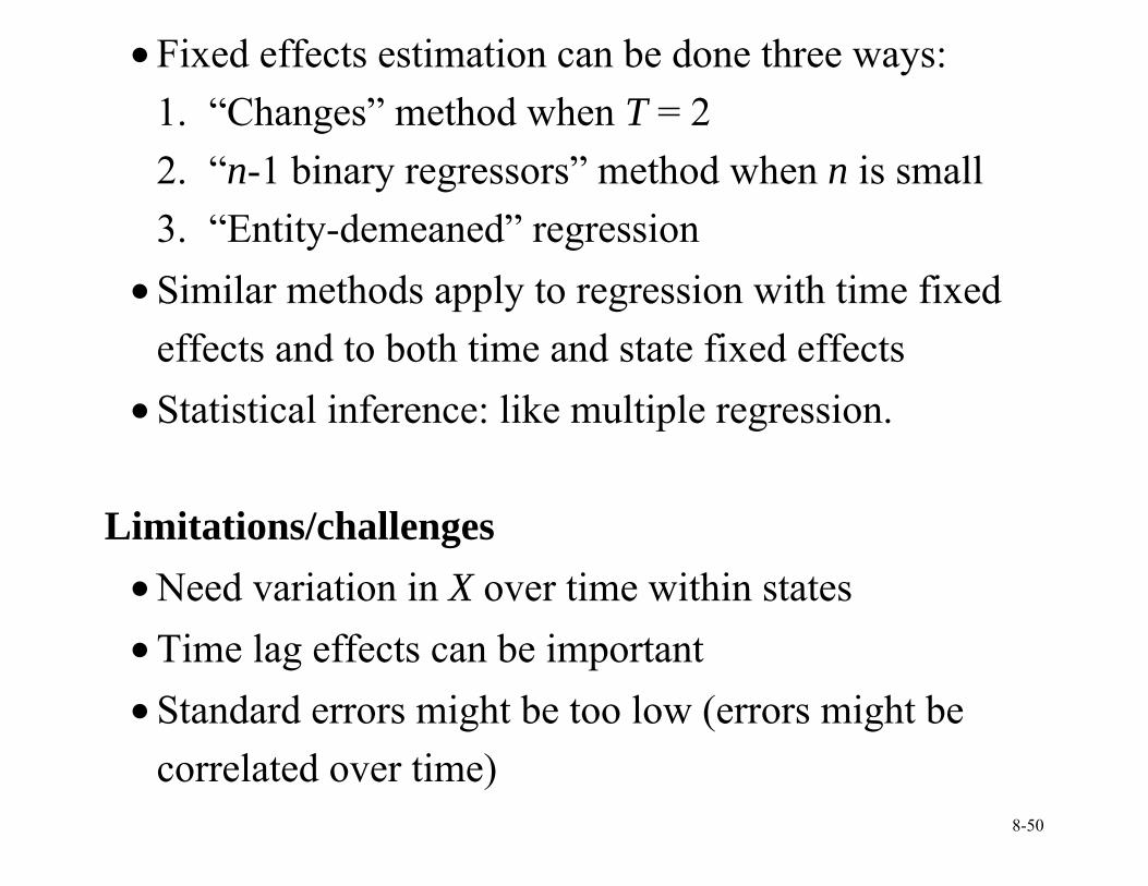
• Fixed effects estimation can be done three ways: 1. “Changes” method when T = 2 2. “n-1 binary regressors” method when n is small 3. “Entity-demeaned” regression

• Similar methods apply to regression with time fixed effects and to both time and state fixed effects

• Statistical inference: like multiple regression. Limitations/challenges

• Need variation in X over time within states • Time lag effects can be important • Standard errors might be too low (errors might be

correlated over time)