Ch 6Sampling and Analog-to-Digital Conversion

ENGR 4323/5323Digital and Analog Communication

Engineering and PhysicsUniversity of Central Oklahoma

Dr. Mohamed Bingabr

Chapter Outline

• Sampling Theorem

• Pulse Code Modulation (PCM)

• Digital Telephony: PCM IN T1 Carrier Systems

• Digital Multiplexing

• Differential Pulse Code Modulation (DPCM)

• Adaptive Differential PCM (ADPCM)

• Delta Modulation

• Vocoders and Video Compression2

Sampling Theorem

Sampling is the first step in converting a continuous signal to a

digital signal.

Sampling Theorem determines the minimum number of

samples needed to reconstruct perfectly the continuous signal

again from its samples.

Sampling Theorem: A continuous function x(t) bandlimited to B

Hz can be reconstructed from its samples if it was sampled at

rate equal or greater than 2 B samples per second. If the

sampling rate equals 2 B then it is called the Nyquist rate.3

Sampling Theorem

4

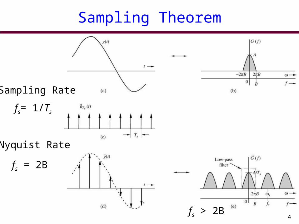
Sampling Rate

fs = 2B

fs= 1/Ts

Nyquist Rate

fs > 2B

Sampling Theorem

5

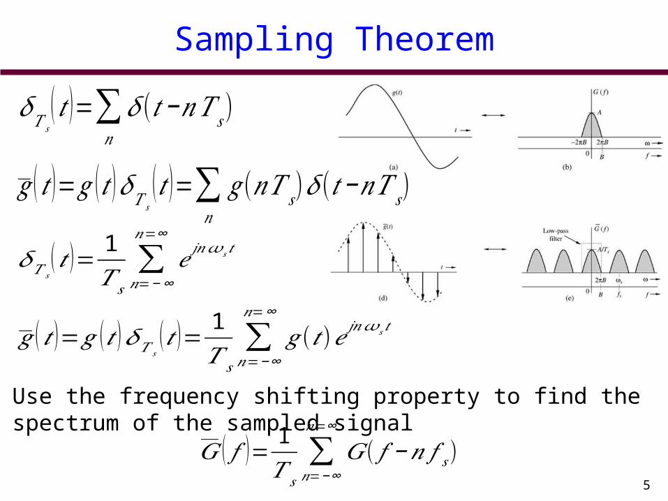
𝛿𝑇 𝑠(𝑡 )=∑

𝑛

𝛿(𝑡−𝑛𝑇 𝑠)

𝑔 (𝑡 )=𝑔 (𝑡 )𝛿𝑇 𝑠(𝑡 )=∑

𝑛

𝑔(𝑛𝑇 𝑠)𝛿(𝑡−𝑛𝑇 𝑠)

𝛿𝑇 𝑠(𝑡 )= 1

𝑇 𝑠∑

𝑛=−∞

𝑛=∞

𝑒 𝑗𝑛𝜔 𝑠𝑡

𝑔 (𝑡 )=𝑔 (𝑡 )𝛿𝑇 𝑠(𝑡 )= 1

𝑇 𝑠∑𝑛=− ∞

𝑛=∞

𝑔(𝑡)𝑒 𝑗𝑛 𝜔𝑠𝑡

Use the frequency shifting property to find the spectrum of the sampled signal

𝐺 ( 𝑓 )= 1𝑇 𝑠

∑𝑛=− ∞

𝑛=∞

𝐺( 𝑓 −𝑛 𝑓 𝑠)

Reconstruction from Uniform Samples

6

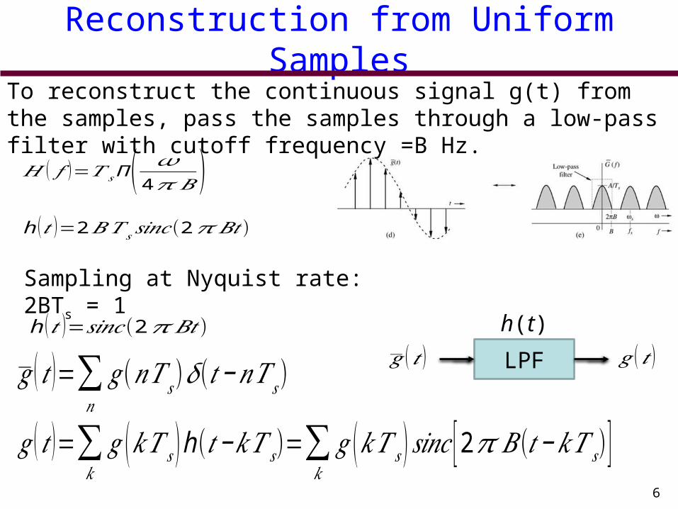
𝐻 ( 𝑓 )=𝑇 𝑠Π ( 𝜔4𝜋 𝐵 )

h (𝑡 )=2𝐵𝑇 𝑠𝑠𝑖𝑛𝑐(2𝜋 𝐵𝑡)

To reconstruct the continuous signal g(t) from the samples, pass the samples through a low-pass filter with cutoff frequency =B Hz.

h (𝑡 )=𝑠𝑖𝑛𝑐(2𝜋 𝐵𝑡 )

Sampling at Nyquist rate: 2BTs = 1

LPF𝑔 (𝑡 )=∑𝑛

𝑔(𝑛𝑇 𝑠)𝛿(𝑡−𝑛𝑇 𝑠)𝑔 (𝑡 ) 𝑔 (𝑡 )

𝑔 (𝑡 )=∑𝑘

𝑔 (𝑘𝑇 𝑠 ) h (𝑡−𝑘𝑇 𝑠)=∑𝑘

𝑔 (𝑘𝑇 𝑠 )𝑠𝑖𝑛𝑐 [2𝜋 𝐵(𝑡−𝑘𝑇𝑠) ]

h(t)

Reconstruction from Uniform Samples

7

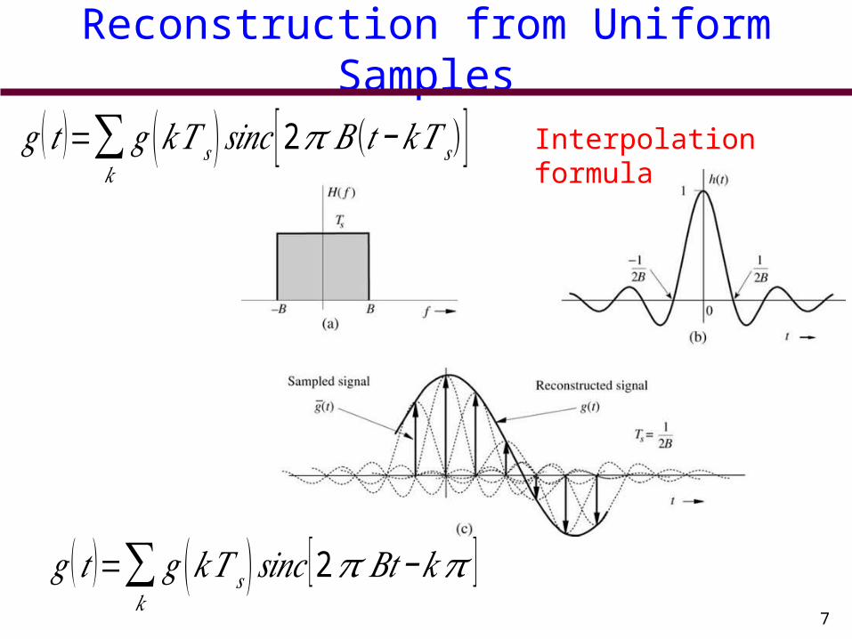
𝑔 (𝑡 )=∑𝑘

𝑔 (𝑘𝑇 𝑠 ) 𝑠𝑖𝑛𝑐 [ 2𝜋 𝐵𝑡−𝑘𝜋 ]

𝑔 (𝑡 )=∑𝑘

𝑔 (𝑘𝑇 𝑠 ) 𝑠𝑖𝑛𝑐 [2𝜋 𝐵(𝑡−𝑘𝑇 𝑠)] Interpolation formula

Example 6.1

8

Find a signal g(t) that is band-limited to B Hz and whose samples are g(0) = 1 and g(±Ts) = g(±2Ts) = g(±3Ts) =…= 0 where the sampling interval Ts is the Nyquist interval, that is Ts = 1/2B.

Practical Signal Reconstruction

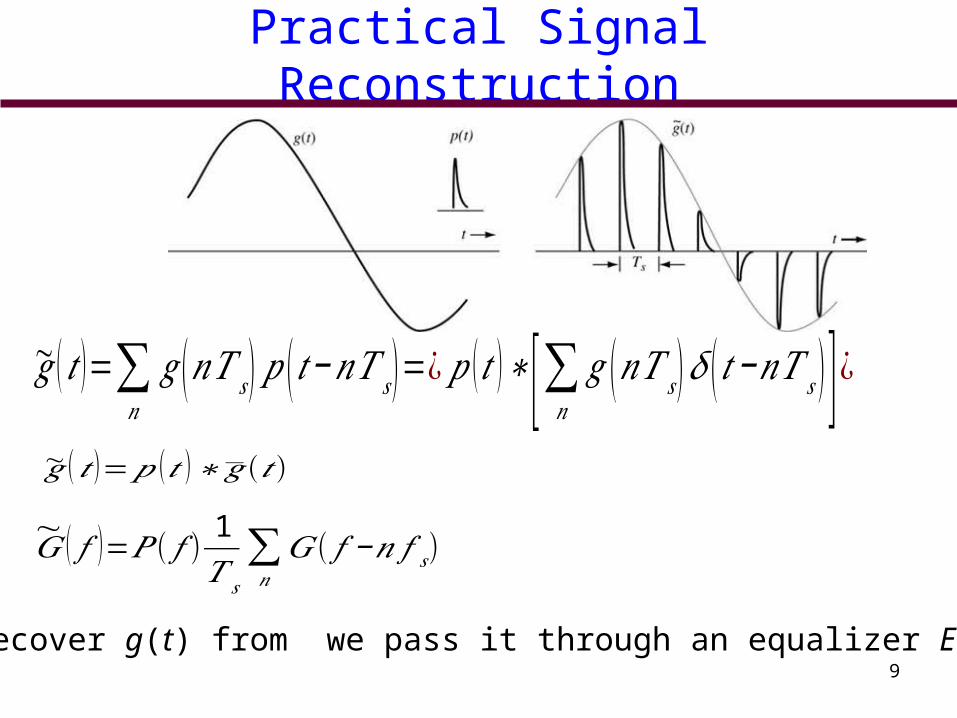
~𝑔 (𝑡 )=∑𝑛

𝑔 (𝑛𝑇 𝑠 )𝑝 ( 𝑡−𝑛𝑇 𝑠 )=¿𝑝 (𝑡 )∗[∑𝑛 𝑔 (𝑛𝑇 𝑠 ) 𝛿 ( 𝑡−𝑛𝑇 𝑠 ) ]¿~𝑔 (𝑡 )=𝑝 (𝑡 )∗𝑔 (𝑡)

~𝐺 ( 𝑓 )=𝑃 ( 𝑓 )

1𝑇 𝑠

∑𝑛

𝐺( 𝑓 −𝑛 𝑓 𝑠)

To recover g(t) from we pass it through an equalizer E( f )9

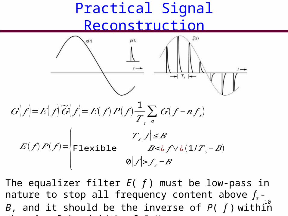
Practical Signal Reconstruction

𝐺 ( 𝑓 )=𝐸 ( 𝑓 )~𝐺 ( 𝑓 )=𝐸 ( 𝑓 )𝑃 ( 𝑓 )1𝑇 𝑠

∑𝑛

𝐺 ( 𝑓 −𝑛 𝑓 𝑠)

𝐸 ( 𝑓 )𝑃 ( 𝑓 )={ 𝑇 𝑠|𝑓 |≤𝐵Flexible      𝐵<¿ 𝑓∨¿(1 /𝑇 𝑠−𝐵)

0|𝑓 |> 𝑓 𝑠−𝐵

The equalizer filter E( f ) must be low-pass in nature to stop all frequency content above fs - B, and it should be the inverse of P( f ) within the signal bandwidth of B Hz.

10

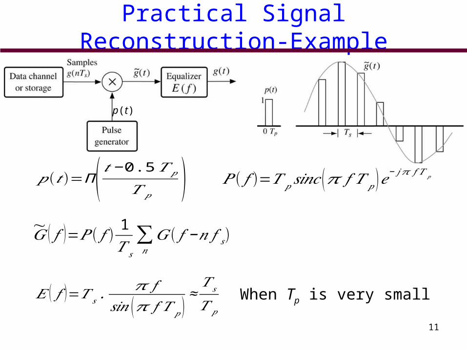
Practical Signal Reconstruction-Example

11

𝑝 (𝑡)=Π ( 𝑡− 0.5𝑇𝑝

𝑇 𝑝)

~𝐺 ( 𝑓 )=𝑃 ( 𝑓 )

1𝑇 𝑠

∑𝑛

𝐺( 𝑓 −𝑛 𝑓 𝑠)

𝑃 ( 𝑓 )=𝑇𝑝 𝑠𝑖𝑛𝑐 (𝜋 𝑓 𝑇 𝑝)𝑒− 𝑗 𝜋 𝑓 𝑇 𝑝

𝐸 ( 𝑓 )=𝑇 𝑠 .𝜋 𝑓

𝑠𝑖𝑛 (𝜋 𝑓 𝑇 𝑝)≈𝑇 𝑠

𝑇 𝑝

When Tp is very small

p(t)

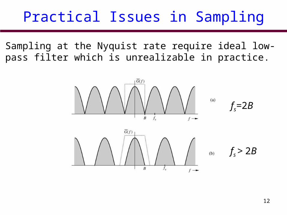
Practical Issues in Sampling

Sampling at the Nyquist rate require ideal low-pass filter which is unrealizable in practice.

fs=2B

fs > 2B

12

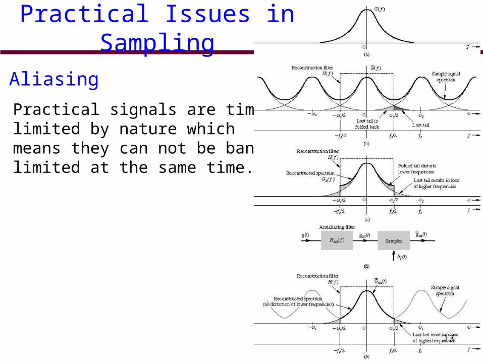
Aliasing

Practical signals are time-limited by nature which means they can not be band-limited at the same time.

Practical Issues in Sampling

13

Maximum Information Rate

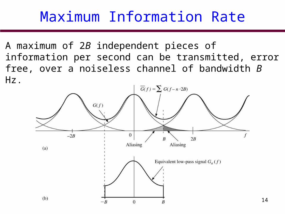
A maximum of 2B independent pieces of information per second can be transmitted, error free, over a noiseless channel of bandwidth B Hz.

14

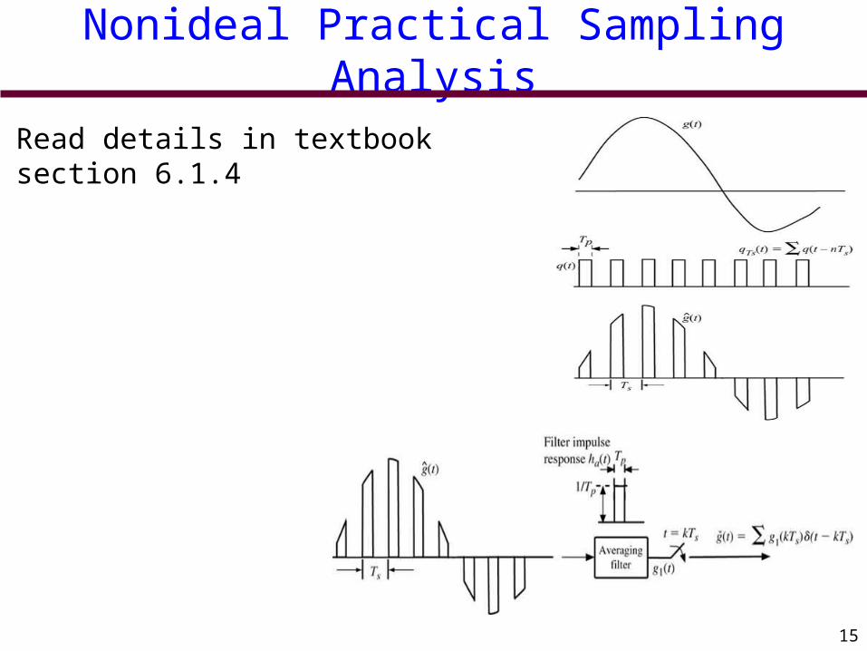
Nonideal Practical Sampling Analysis

Read details in textbook section 6.1.4

15

Sampling Theorem and Pulse Modulation

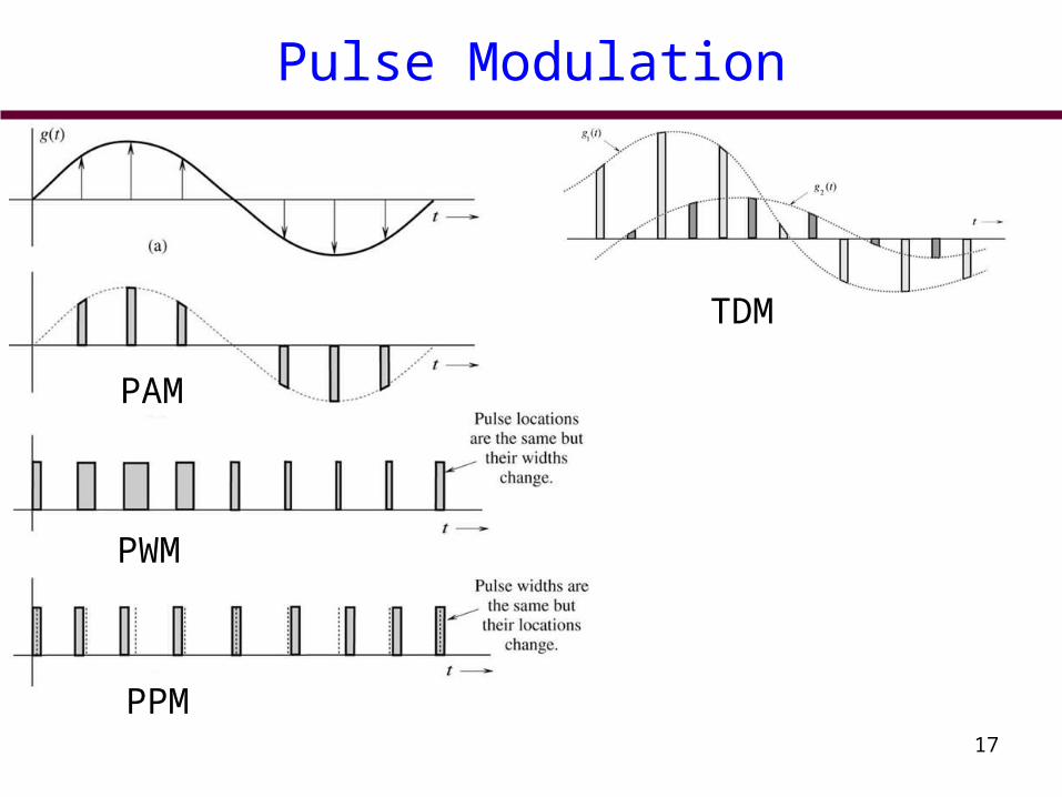
The continuous signal g(t) is sampled, and sample values are used to modify certain parameters (amplitude, width, position) of a periodic pulse train.

Techniques for communication using pulse modulation:

1- Pulse Amplitude Modulation (PAM)

2- Pulse Width Modulation (PWM)

3- Pulse Position Modulation (PPM)

4- Pulse Code Modulation (PCM)

5- Time Division Multiplexing (TDM)

16

Pulse Modulation

TDM

PWM

PAM

PPM17

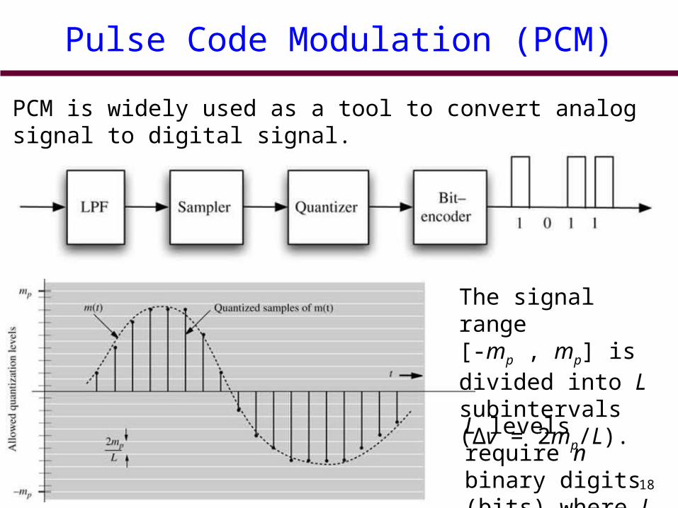
Pulse Code Modulation (PCM)

PCM is widely used as a tool to convert analog signal to digital signal.

The signal range [-mp , mp] is divided into L subintervals (Δv = 2mp/L).

L levels require n binary digits (bits) where L = 2n. 18

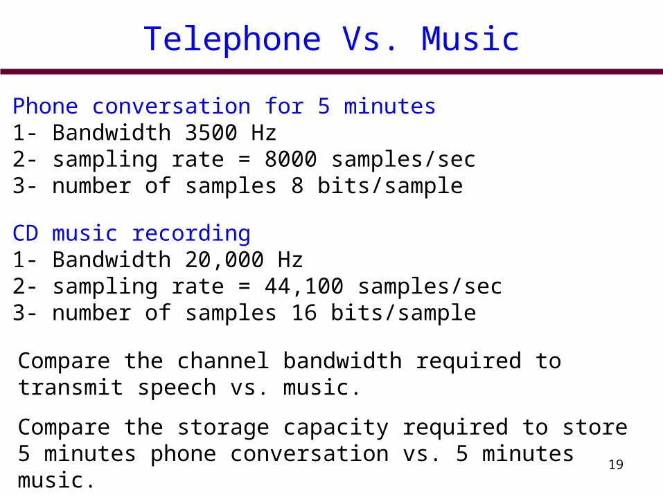
Telephone Vs. Music

Phone conversation for 5 minutes1- Bandwidth 3500 Hz2- sampling rate = 8000 samples/sec3- number of samples 8 bits/sample

CD music recording1- Bandwidth 20,000 Hz2- sampling rate = 44,100 samples/sec3- number of samples 16 bits/sample

Compare the channel bandwidth required to transmit speech vs. music.

Compare the storage capacity required to store 5 minutes phone conversation vs. 5 minutes music.

19

Advantage of Digital Communication

1) Withstand channel noise and distortion much better than analog.

2) With regenerative repeater it is possible to transmit over long distance.

3) Digital hardware implementation is flexible4) Digital coding provide further error reduction, high fidelity and

privacy.5) Easier to multiplex several digital signals.6) More efficient in exchanging SNR for bandwidth.7) Digital signal storage is relatively easy and inexpensive.8) Reproduction with digital messages is reliable without

deterioration.9) Cost of digital hardware is cheaper and continue to decrease.

20

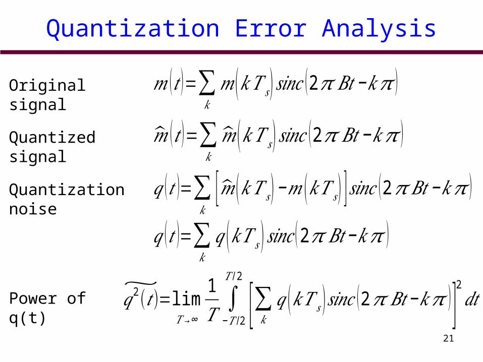
Quantization Error Analysis

Original signal 𝑚 (𝑡 )=∑𝑘

𝑚 (𝑘𝑇 𝑠 ) 𝑠𝑖𝑛𝑐 (2𝜋 𝐵𝑡−𝑘𝜋 )

Quantized signal �̂� (𝑡 )=∑𝑘

�̂� (𝑘𝑇 𝑠 ) 𝑠𝑖𝑛𝑐 (2𝜋 𝐵𝑡−𝑘𝜋 )

Quantization noise 𝑞 (𝑡 )=∑𝑘

[�̂� (𝑘𝑇 𝑠 )−𝑚 (𝑘𝑇 𝑠 ) ]𝑠𝑖𝑛𝑐 (2𝜋 𝐵𝑡−𝑘 𝜋 )

𝑞 (𝑡 )=∑𝑘

𝑞 (𝑘𝑇 𝑠 )𝑠𝑖𝑛𝑐 (2𝜋 𝐵𝑡−𝑘𝜋 )

Power of q(t)~𝑞2(𝑡)= lim

𝑇 → ∞

1𝑇 ∫

−𝑇 /2

𝑇 /2

[∑𝑘 𝑞 (𝑘𝑇 𝑠 ) 𝑠𝑖𝑛𝑐 (2𝜋 𝐵𝑡−𝑘𝜋 ) ]2𝑑𝑡

21

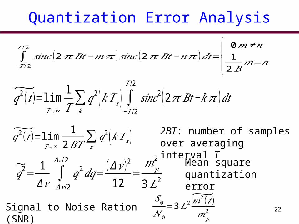
Quantization Error Analysis

∫−𝑇 /2

𝑇 /2

𝑠𝑖𝑛𝑐 (2𝜋 𝐵𝑡−𝑚𝜋 ) 𝑠𝑖𝑛𝑐 (2𝜋 𝐵𝑡−𝑛𝜋 )𝑑𝑡={ 0𝑚≠𝑛1

2𝐵𝑚=𝑛

~𝑞2(𝑡)= lim

𝑇 → ∞

1𝑇∑

𝑘

𝑞2 (𝑘𝑇 𝑠 ) ∫−𝑇 /2

𝑇 /2

𝑠𝑖𝑛𝑐2 (2𝜋 𝐵𝑡−𝑘𝜋 )𝑑𝑡

~𝑞2(𝑡)= lim

𝑇 → ∞

12𝐵𝑇 ∑

𝑘

𝑞2 (𝑘𝑇 𝑠 ) 2BT: number of samples over averaging interval T

Mean square quantization error

~𝑞2= 1

∆ 𝑣 ∫− ∆𝑣 /2

∆ 𝑣/2

𝑞2𝑑𝑞=(∆𝑣 )2

12=𝑚𝑝

2

3𝐿2

𝑆0

𝑁0

=3𝐿2

~𝑚2(𝑡)𝑚𝑝

2Signal to Noise Ration (SNR) 22

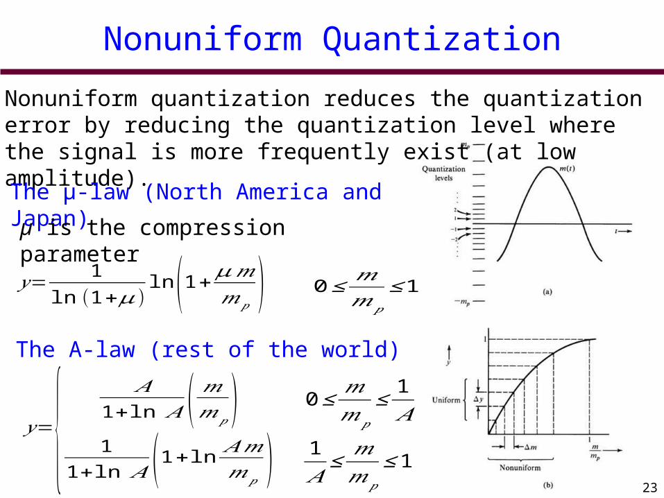
Nonuniform Quantization

Nonuniform quantization reduces the quantization error by reducing the quantization level where the signal is more frequently exist (at low amplitude).

The µ-law (North America and Japan)

𝑦=1

ln (1+𝜇)ln(1+

𝜇𝑚𝑚𝑝

) 0 ≤𝑚𝑚𝑝

≤ 1

The A-law (rest of the world)

𝑦={ 𝐴1+ ln 𝐴 ( 𝑚𝑚𝑝

)1

1+ln 𝐴 (1+ ln𝐴𝑚𝑚𝑝

)0 ≤

𝑚𝑚𝑝

≤1𝐴

1𝐴

≤𝑚𝑚𝑝

≤ 123

µ is the compression parameter

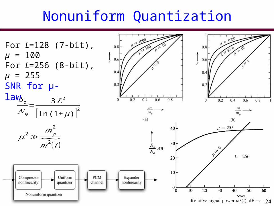
Nonuniform Quantization

SNR for µ-law𝑆0

𝑁0

= 3𝐿2

[ ln (1+ μ )]2

𝜇2≫𝑚𝑝

2

~𝑚2(𝑡)

24

For L=128 (7-bit), µ = 100For L=256 (8-bit), µ = 255

Transmission Bandwidth

B : Signal bandwidth in HzL : Quantization Leveln : Number of bits per samplefs : Samples per secondBT: Transmission Channel Bandwidth

fs = 2*Bn = log2 L Number of bits per second = 2*B*nBT = Number of bits per second /2;BT = B*n

Usually the sampling rate is higher than the Nyquest rate 2B to improve signal to noise ratio (SNR). 25

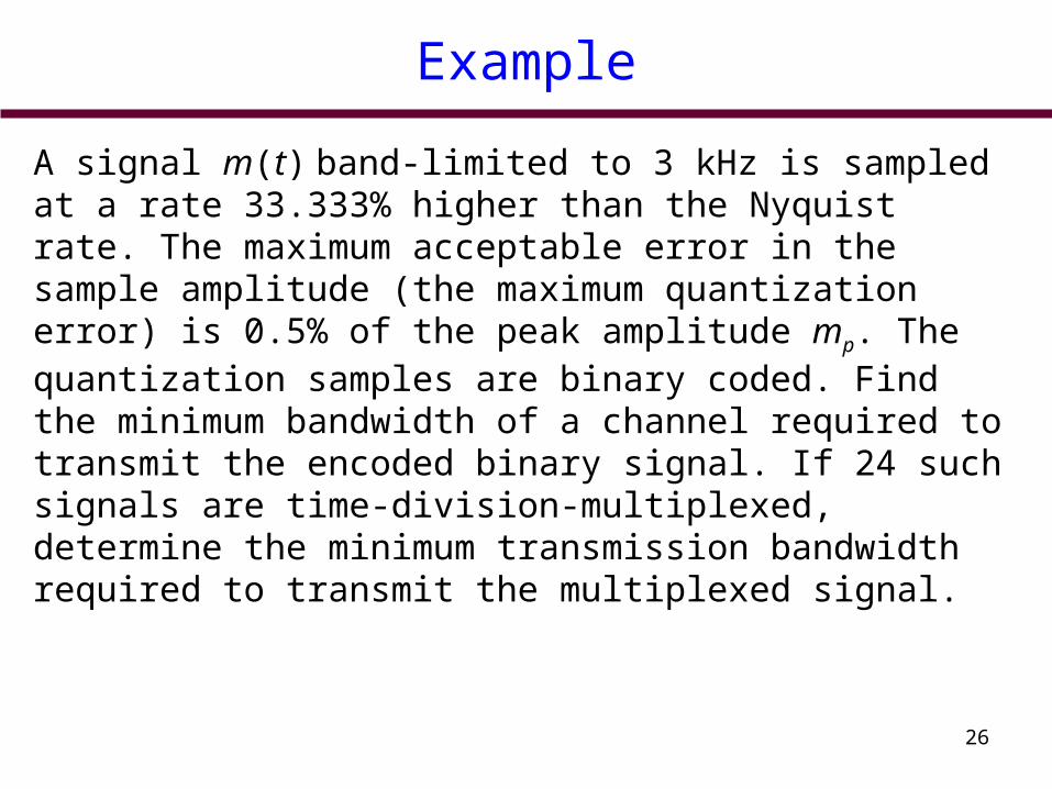
Example

A signal m(t) band-limited to 3 kHz is sampled at a rate 33.333% higher than the Nyquist rate. The maximum acceptable error in the sample amplitude (the maximum quantization error) is 0.5% of the peak amplitude mp. The quantization samples are binary coded. Find the minimum bandwidth of a channel required to transmit the encoded binary signal. If 24 such signals are time-division-multiplexed, determine the minimum transmission bandwidth required to transmit the multiplexed signal.

26

Channel Bandwidth and SNR

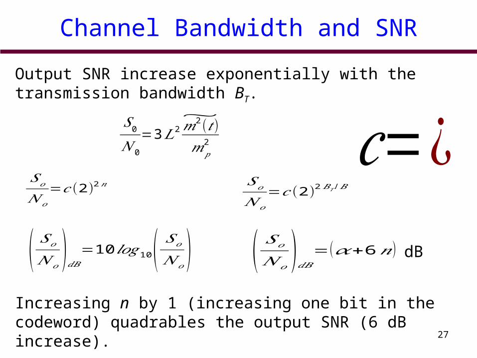
Output SNR increase exponentially with the transmission bandwidth BT.

𝑆𝑜

𝑁𝑜

=𝑐 (2)2𝑛

𝑐=¿𝑆𝑜

𝑁𝑜

=𝑐 (2)2 𝐵𝑇 /𝐵

( 𝑆𝑜

𝑁𝑜)𝑑𝐵

=10 𝑙𝑜𝑔10( 𝑆𝑜

𝑁 𝑜) ( 𝑆𝑜

𝑁𝑜)𝑑𝐵

=(𝛼+6𝑛) dB

Increasing n by 1 (increasing one bit in the codeword) quadrables the output SNR (6 dB increase).

27

𝑆0

𝑁0

=3𝐿2

~𝑚2(𝑡)𝑚𝑝

2

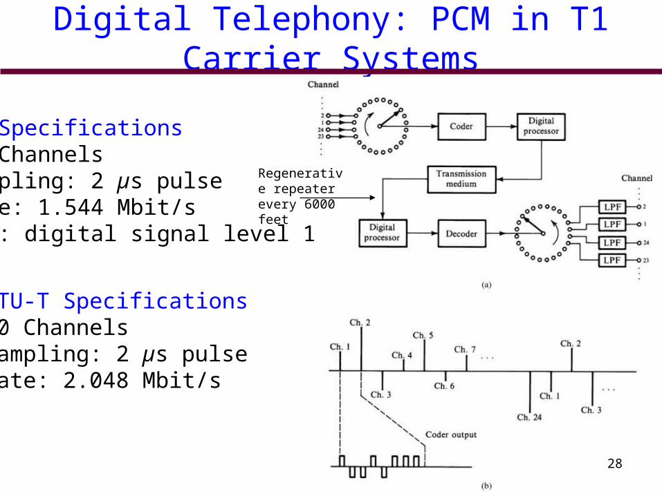
Digital Telephony: PCM in T1 Carrier Systems

Regenerative repeater every 6000 feet

T1 Specifications24 ChannelsSampling: 2 µs pulseRate: 1.544 Mbit/sDS1: digital signal level 1

ITU-T Specifications30 ChannelsSampling: 2 µs pulseRate: 2.048 Mbit/s

28

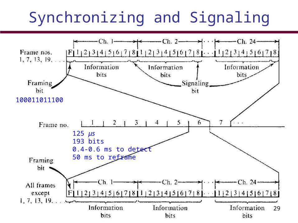
Synchronizing and Signaling

29

100011011100

125 μs193 bits0.4-0.6 ms to detect50 ms to reframe

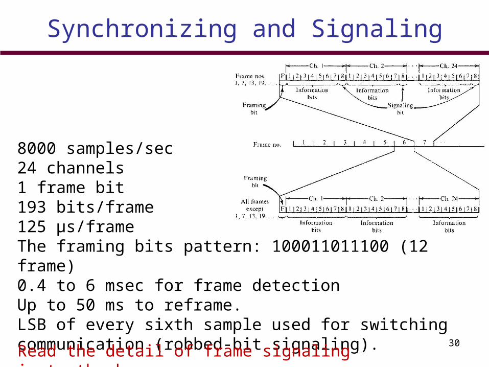
Synchronizing and Signaling

8000 samples/sec24 channels1 frame bit193 bits/frame125 µs/frameThe framing bits pattern: 100011011100 (12 frame)0.4 to 6 msec for frame detectionUp to 50 ms to reframe.LSB of every sixth sample used for switching communication (robbed-bit signaling).

Read the detail of frame signaling in textbook30

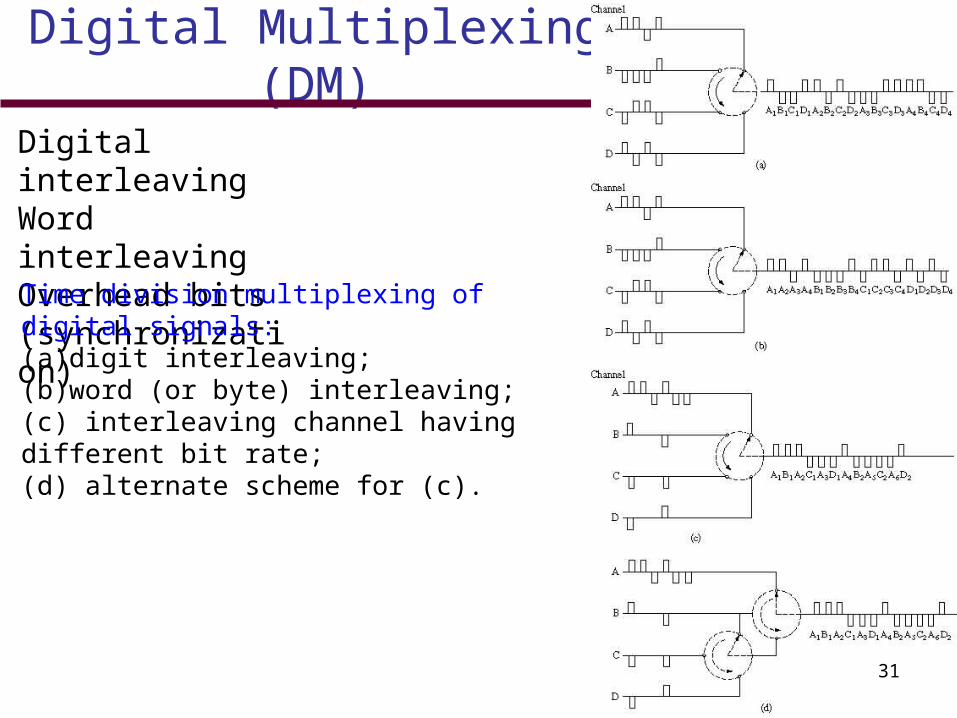
Digital Multiplexing (DM)

Digital interleavingWord interleavingOverhead bits (synchronization)

Time division multiplexing of digital signals: (a) digit interleaving; (b) word (or byte) interleaving;(c) interleaving channel having different bit rate; (d) alternate scheme for (c).

31

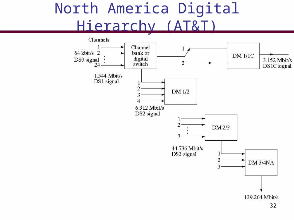
North America Digital Hierarchy (AT&T)

32

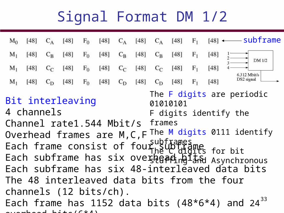
Signal Format DM 1/2

Bit interleaving4 channelsChannel rate1.544 Mbit/sOverhead frames are M,C,FEach frame consist of four subframe Each subframe has six overhead bitsEach subframe has six 48-interleaved data bitsThe 48 interleaved data bits from the four channels (12 bits/ch). Each frame has 1152 data bits (48*6*4) and 24 overhead bits(6*4).Efficiency =1152/1176=98%

The F digits are periodic 01010101F digits identify the framesThe M digits 0111 identify subframesThe C digits for bit stuffing and Asynchronous

33

subframe

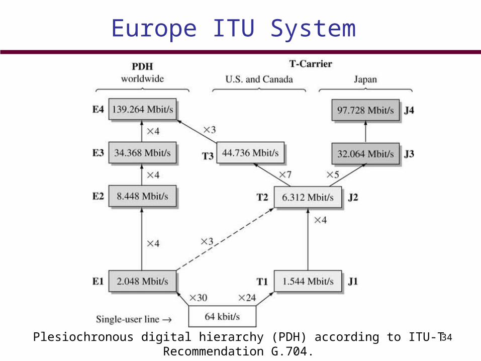
Europe ITU System

Plesiochronous digital hierarchy (PDH) according to ITU-T Recommendation G.704.34

Differential Pulse Code Modulation (DPCM)

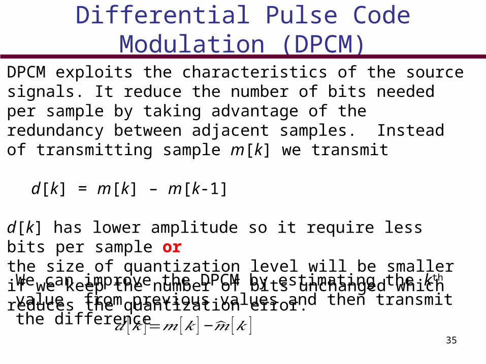
DPCM exploits the characteristics of the source signals. It reduce the number of bits needed per sample by taking advantage of the redundancy between adjacent samples. Instead of transmitting sample m[k] we transmit

d[k] = m[k] – m[k-1]

d[k] has lower amplitude so it require less bits per sample or the size of quantization level will be smaller if we keep the number of bits unchanged which reduces the quantization error.

We can improve the DPCM by estimating the kth value from previous values and then transmit the difference

35𝑑 [𝑘 ]=𝑚 [𝑘 ] −�̂� [𝑘 ]

Differential Pulse Code Modulation (DPCM)

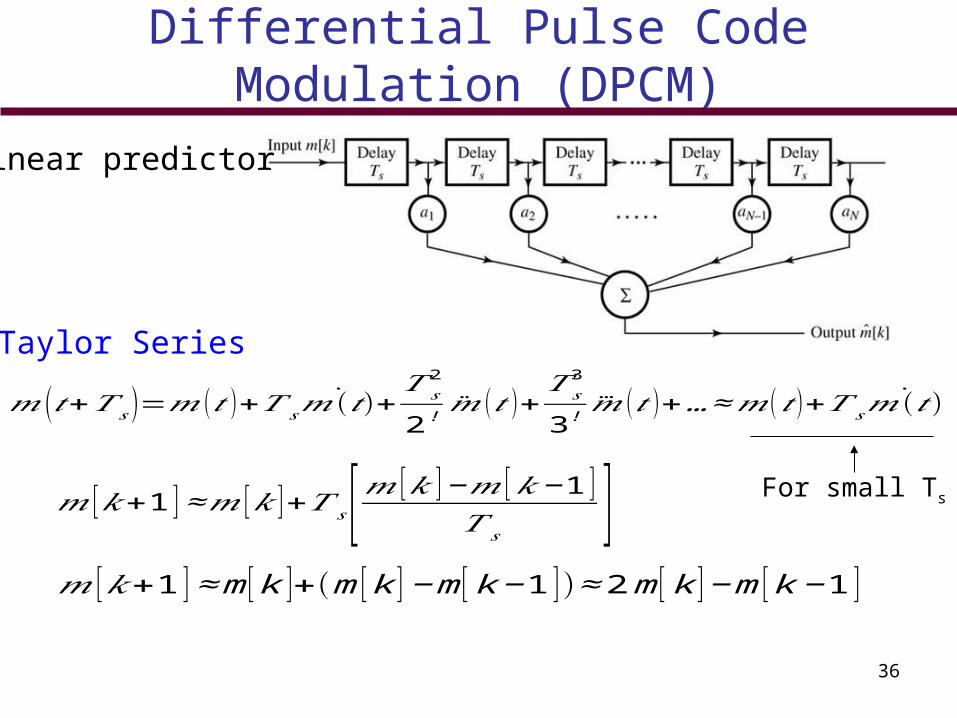
Linear predictor

𝑚 (𝑡+𝑇 𝑠 )=𝑚 (𝑡 )+𝑇 𝑠˙𝑚(𝑡)+

𝑇 𝑠2

2! �̈� (𝑡 )+𝑇 𝑠

3

3! �⃛� (𝑡 )+…≈𝑚 (𝑡 )+𝑇 𝑠˙𝑚(𝑡)

𝑚 [𝑘+1 ] ≈𝑚 [𝑘 ]+𝑇 𝑠 [𝑚 [𝑘 ] −𝑚 [𝑘−1 ]𝑇 𝑠 ]

𝑚 [𝑘+1 ] ≈ m [ k ]+(m [ k ] −m [ k − 1 ])≈ 2 m [ k ] −m [ k −1 ]

36

Taylor Series

For small Ts

Analysis of DPCM

37

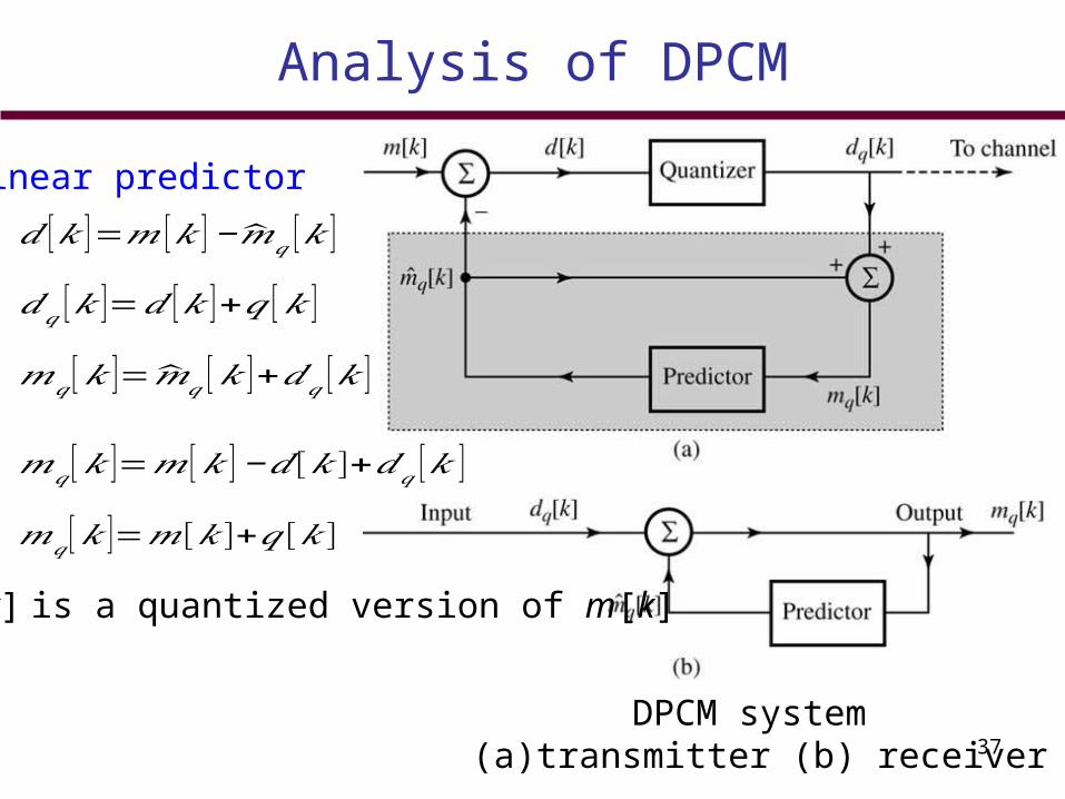
Linear predictor

𝑑 [𝑘 ]=𝑚 [𝑘 ] −�̂�𝑞 [𝑘 ]

𝑑𝑞 [𝑘 ]=𝑑 [𝑘 ]+𝑞 [𝑘 ]

𝑚𝑞 [𝑘 ]=�̂�𝑞 [𝑘 ]+𝑑𝑞 [𝑘 ]

𝑚𝑞 [𝑘 ]=𝑚 [𝑘 ] −𝑑 [𝑘 ]+𝑑𝑞 [𝑘 ]

𝑚𝑞 [𝑘 ]=𝑚[𝑘]+𝑞 [𝑘]

mq[k] is a quantized version of m[k]

DPCM system (a) transmitter (b) receiver

Adaptive Differential PCM (ADPCM)

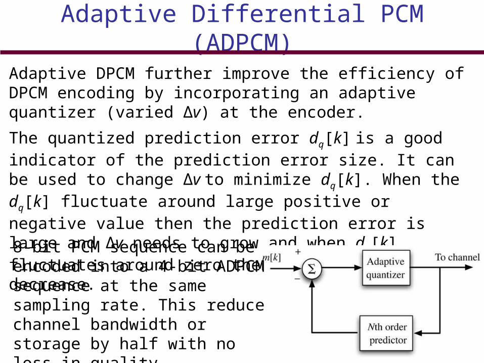
Adaptive DPCM further improve the efficiency of DPCM encoding by incorporating an adaptive quantizer (varied Δv) at the encoder.

The quantized prediction error dq[k] is a good indicator of the prediction error size. It can be used to change Δv to minimize dq[k]. When the dq[k] fluctuate around large positive or negative value then the prediction error is large and Δv needs to grow and when dq[k] fluctuates around zero then Δv needs to decrease.

8-bit PCM sequence can be encoded into a 4-bit ADPCM sequence at the same sampling rate. This reduce channel bandwidth or storage by half with no loss in quality.

Delta Modulation (DM)

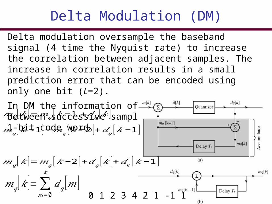
Delta modulation oversample the baseband signal (4 time the Nyquist rate) to increase the correlation between adjacent samples. The increase in correlation results in a small prediction error that can be encoded using only one bit (L=2).

In DM the information of the difference between successive samples is transmitted by a 1-bit code word.

𝑚𝑞 [𝑘 ]=𝑚𝑞 [𝑘−1 ]+𝑑𝑞 [𝑘 ]

𝑚𝑞 [𝑘−1 ]=𝑚𝑞 [𝑘−2 ]+𝑑𝑞 [𝑘− 1 ]

𝑚𝑞 [𝑘 ]=𝑚𝑞 [𝑘− 2 ]+𝑑𝑞 [𝑘 ]+𝑑𝑞 [𝑘− 1 ]

𝑚𝑞 [𝑘 ]=∑𝑚=0

𝑘

𝑑𝑞 [𝑚 ]0 1 2 3 4 2 1 -1 1

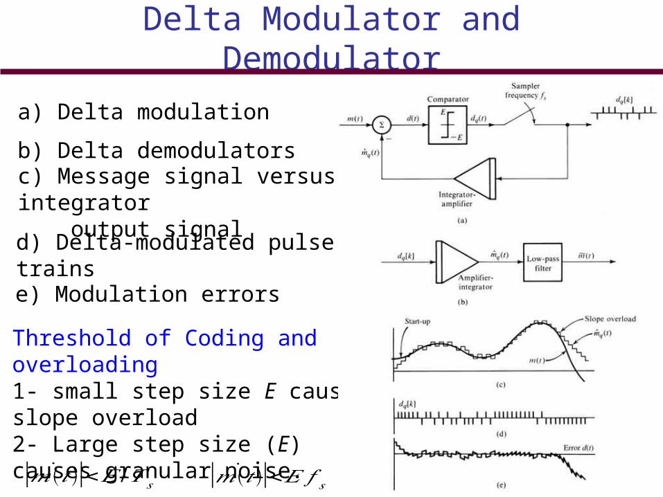
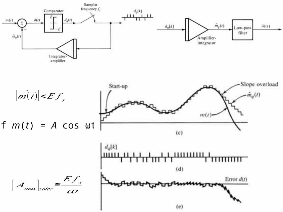
Delta Modulator and Demodulator

a) Delta modulation

b) Delta demodulators

c) Message signal versus integrator output signal

d) Delta-modulated pulse trains

e) Modulation errors

Threshold of Coding and overloading1- small step size E causes slope overload2- Large step size (E) causes granular noise.

| ˙𝑚 (𝑡)|<𝐸 /𝑇 𝑠 | ˙𝑚 (𝑡)|<𝐸 𝑓 𝑠

41

| ˙𝑚 (𝑡)|<𝐸 𝑓 𝑠

If m(t) = A cos ωt

[ 𝐴𝑚𝑎𝑥 ]𝑣𝑜𝑖𝑐𝑒≅𝐸 𝑓 𝑠𝜔

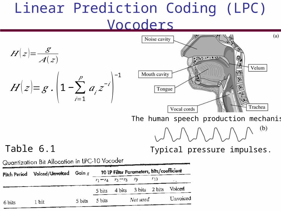
Linear Prediction Coding (LPC) Vocoders

Table 6.1

The human speech production mechanism.

Typical pressure impulses.

𝐻 (𝑧 )= 𝑔𝐴(𝑧)

𝐻 (𝑧 )=𝑔 .(1−∑𝑖=1

𝑝

𝑎𝑖 𝑧−𝑖)

− 1

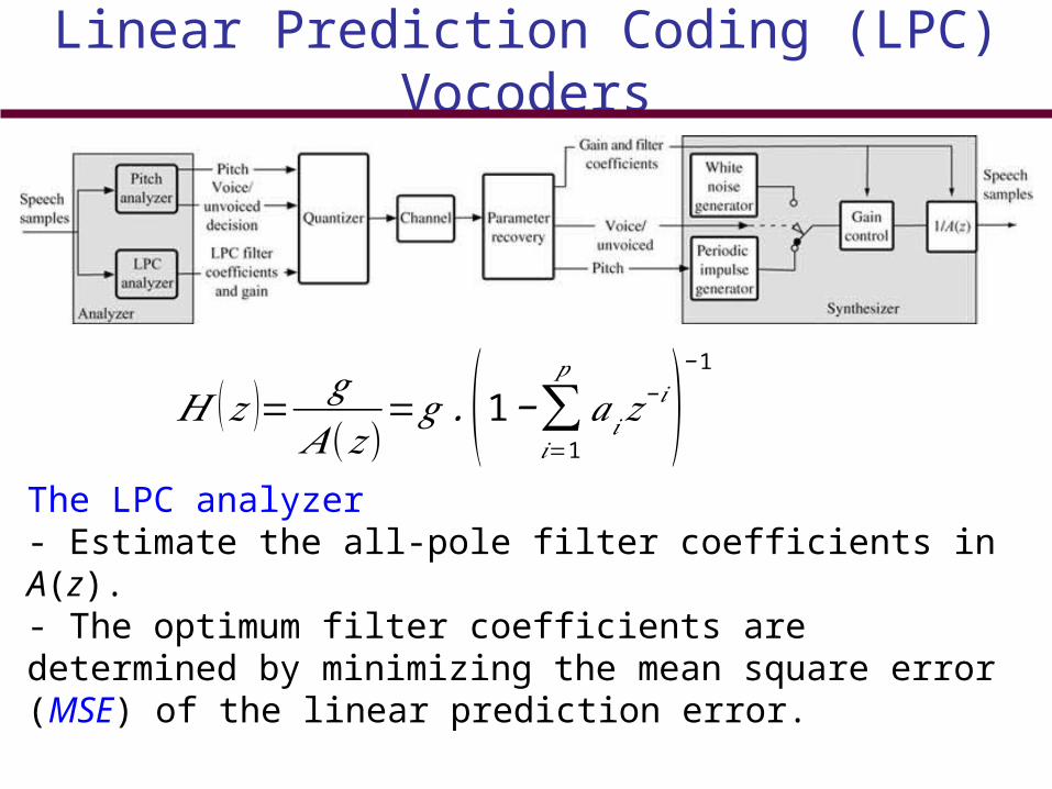
Linear Prediction Coding (LPC) Vocoders

The LPC analyzer - Estimate the all-pole filter coefficients in A(z).- The optimum filter coefficients are determined by minimizing the mean square error (MSE) of the linear prediction error.

𝐻 (𝑧 )= 𝑔𝐴(𝑧)

=𝑔 .(1 −∑𝑖=1

𝑝

𝑎𝑖𝑧−𝑖)

−1

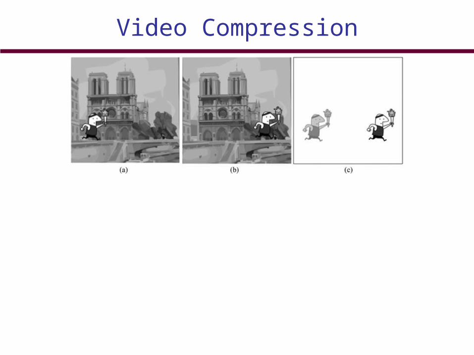
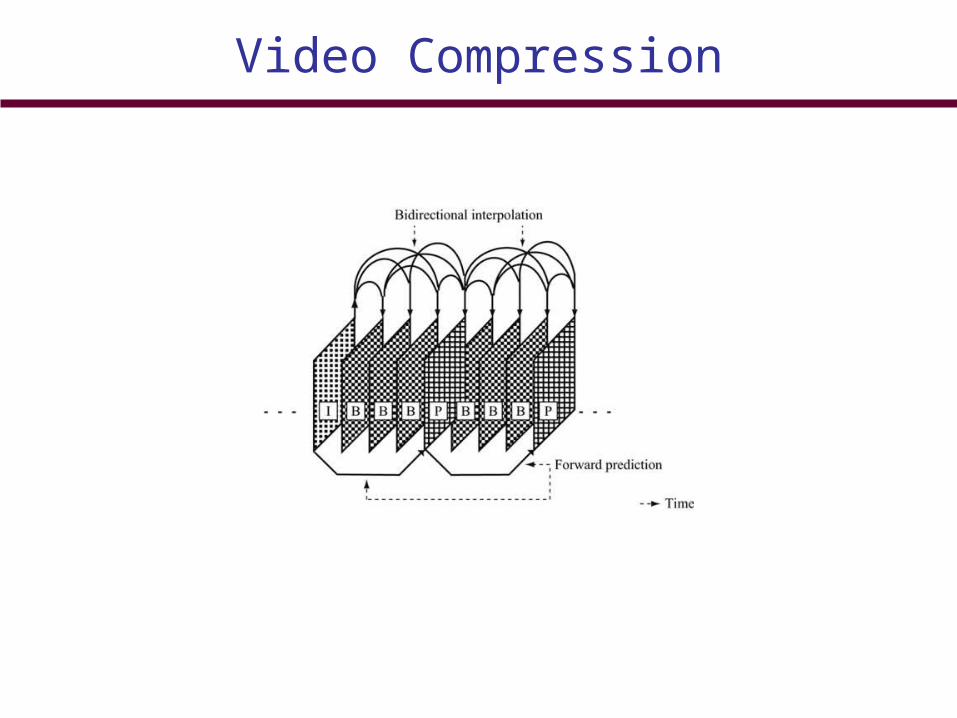
Video Compression

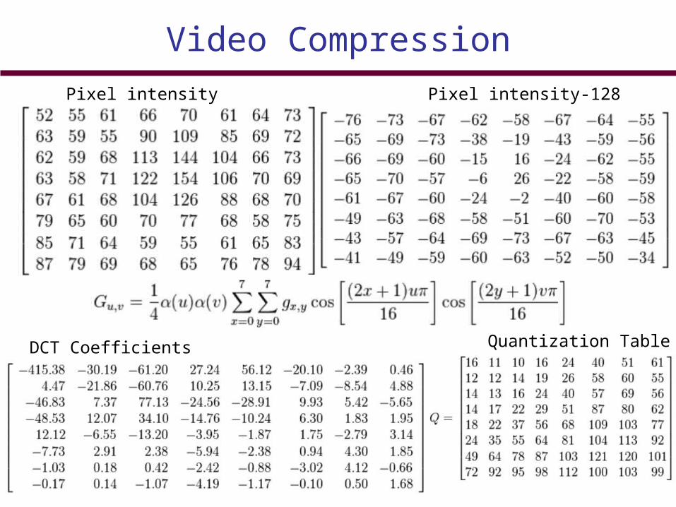
Video Compression

Pixel intensity Pixel intensity-128

DCT Coefficients Quantization Table

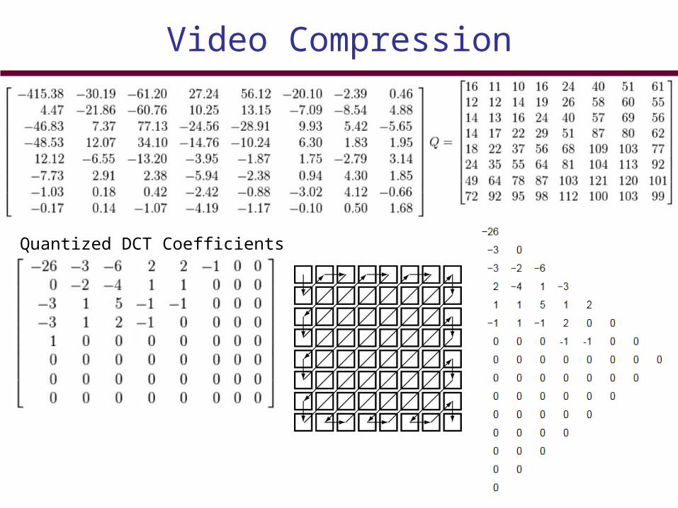
Video Compression

Quantized DCT Coefficients

Video Compression