Embed Size (px)
DESCRIPTION
Ch 5. Profile HMMs for sequence families. Biological sequence analysis: Probabilistic models of proteins and nucleic acids Richard Durbin Sean R. Eddy Anders Krogh Graeme Mitchison. Contents. Components of profile HMMs HMMs from multiple alignments Searching with profile HMMs - PowerPoint PPT Presentation
Citation preview

SNU BioIntelligence Lab. (http://bi.snu.ac.kr) 1
Ch 5. Profile HMMs for sequence families
Biological sequence analysis: Probabilistic models of proteins and nucleic acids
Richard DurbinSean R. EddyAnders KroghGraeme Mitchison
SNU BioIntelligence Lab. (http://bi.snu.ac.kr) 2
Contents
• Components of profile HMMs• HMMs from multiple alignments• Searching with profile HMMs• Variants for non-global alignments• More on estimation probabilities• Optimal model construction• Weighting training sequences
SNU BioIntelligence Lab. (http://bi.snu.ac.kr) 3
Introduction
• Interest on sequence families• Profile HMMs
– Consensus modeling• Theory about inference, learning of profile HM
Ms
SNU BioIntelligence Lab. (http://bi.snu.ac.kr) 4
• figure 5.1
SNU BioIntelligence Lab. (http://bi.snu.ac.kr) 5
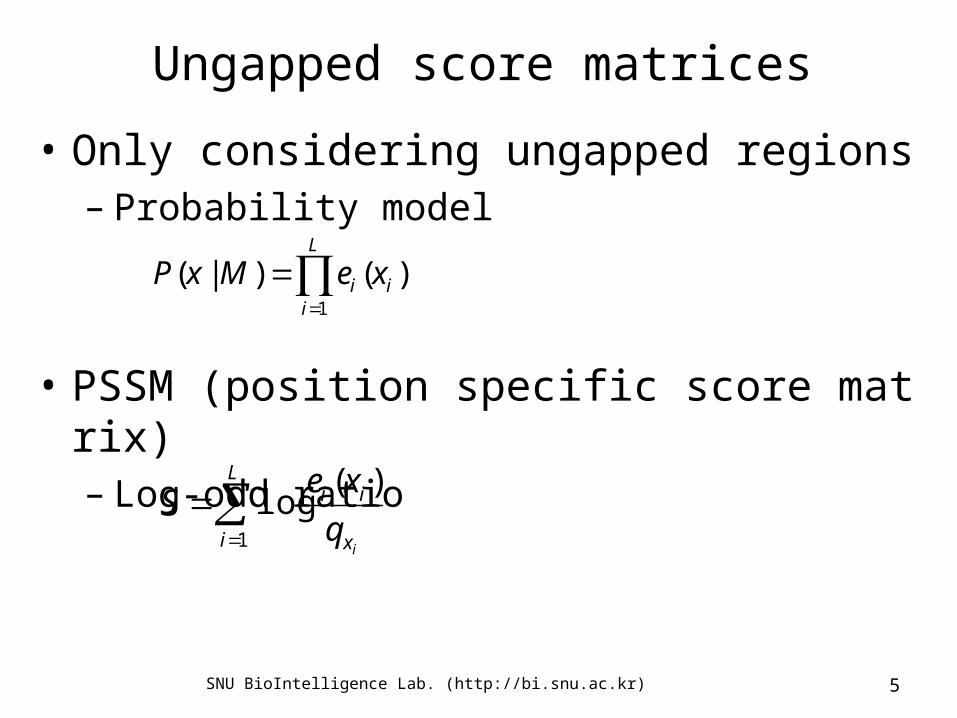
Ungapped score matrices
• Only considering ungapped regions– Probability model
• PSSM (position specific score matrix)– Log-odd ratio
L
iii xeMxP
1
)()|(
L
i x
ii
iq
xeS
1
)(log
SNU BioIntelligence Lab. (http://bi.snu.ac.kr) 6
Components of profile HMMs (1)
• Consideration of gaps– Henikoff & Henikoff [1991]
• Combining the multiple ungapped block models
– Allowing gaps at each position using the same gap scores (g) at each position
• Profile HMMs– Repetitive structure of states– Different probabilities in each position– Full probabilistic model for sequences in the sequ
ence family
SNU BioIntelligence Lab. (http://bi.snu.ac.kr) 7
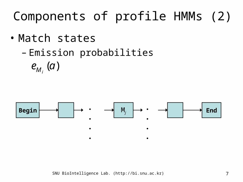
Components of profile HMMs (2)
• Match states– Emission probabilities
Begin Mj End....
..
..
)(aeiM
SNU BioIntelligence Lab. (http://bi.snu.ac.kr) 8
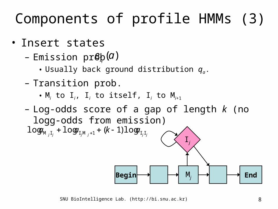
Components of profile HMMs (3)
• Insert states– Emission prob.
• Usually back ground distribution qa.
– Transition prob.• Mi to Ii, Ii to itself, Ii to Mi+1
– Log-odds score of a gap of length k (no logg-odds from emission)
Begin Mj End
Ij
)(I aei
jjjjjjakaa II1MIIM log)1(loglog
SNU BioIntelligence Lab. (http://bi.snu.ac.kr) 9
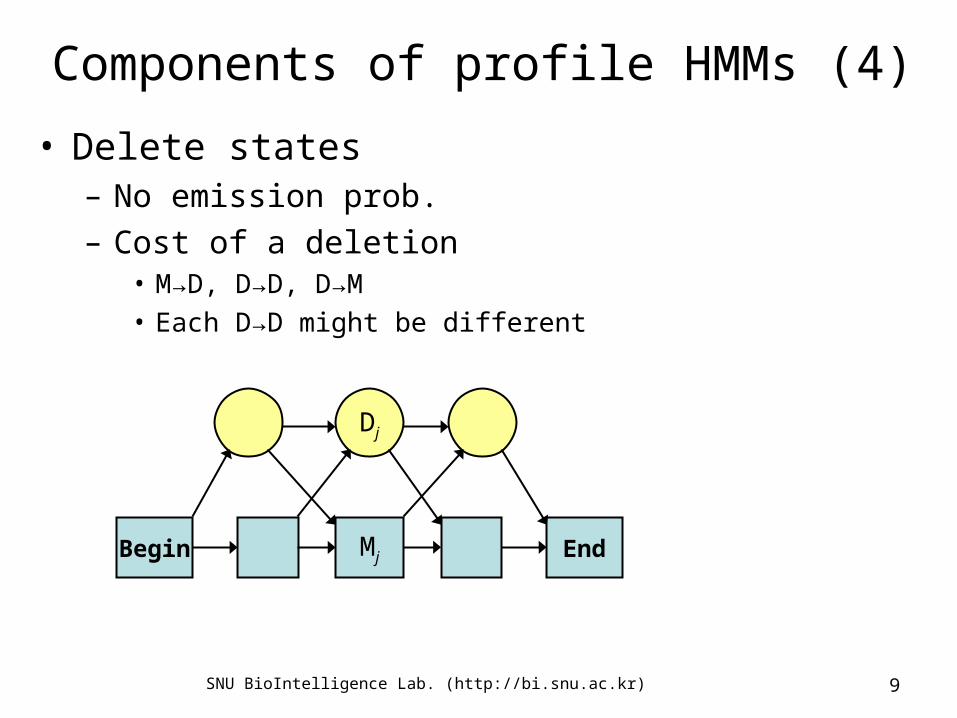
Components of profile HMMs (4)
• Delete states– No emission prob.– Cost of a deletion
• M→D, D→D, D→M• Each D→D might be different
Begin Mj End
Dj
SNU BioIntelligence Lab. (http://bi.snu.ac.kr) 10
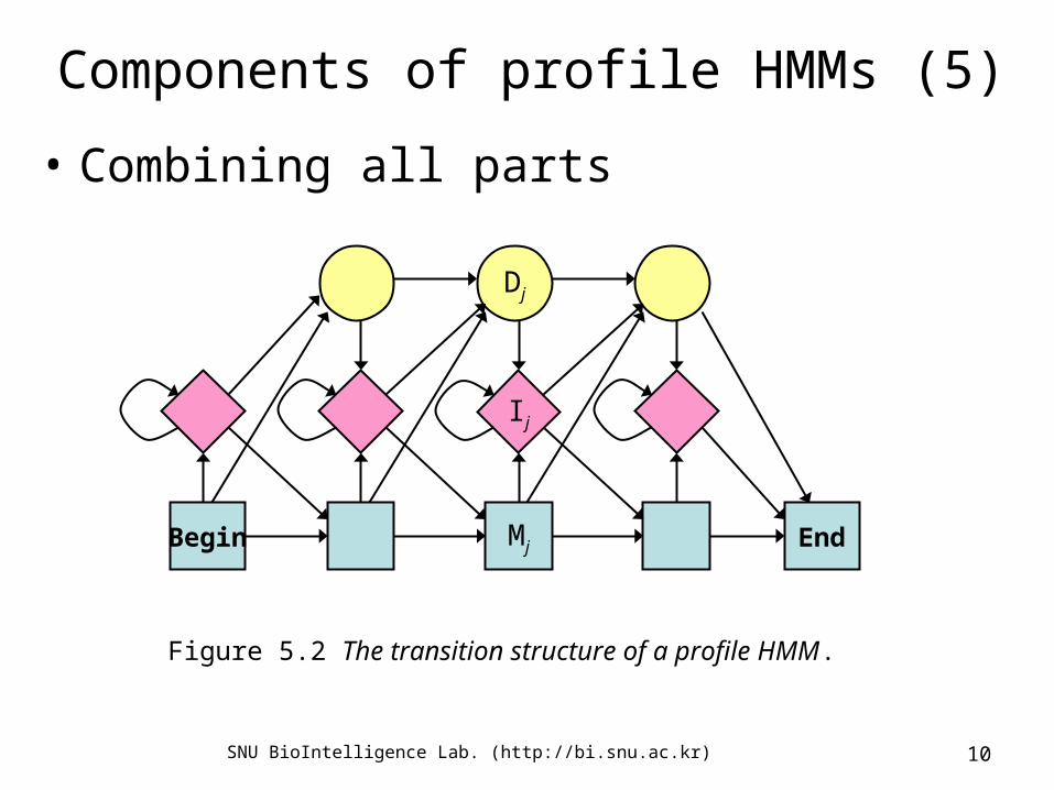
Components of profile HMMs (5)
• Combining all parts
Begin Mj End
Ij
Dj
Figure 5.2 The transition structure of a profile HMM.
SNU BioIntelligence Lab. (http://bi.snu.ac.kr) 11
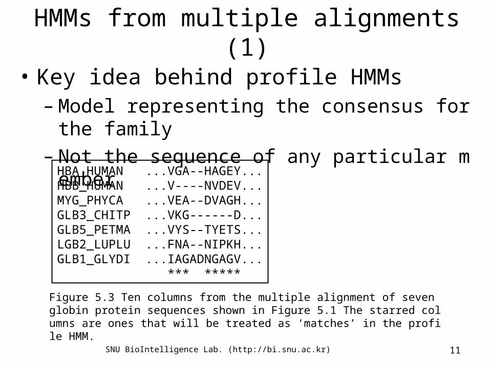
HMMs from multiple alignments (1)
• Key idea behind profile HMMs– Model representing the consensus for the family– Not the sequence of any particular member
HBA_HUMAN ...VGA--HAGEY...HBB_HUMAN ...V----NVDEV...MYG_PHYCA ...VEA--DVAGH...GLB3_CHITP ...VKG------D...GLB5_PETMA ...VYS--TYETS...LGB2_LUPLU ...FNA--NIPKH...GLB1_GLYDI ...IAGADNGAGV... *** *****
Figure 5.3 Ten columns from the multiple alignment of seven globin protein sequences shown in Figure 5.1 The starred columns are ones that will be treated as ‘matches’ in the profile HMM.

SNU BioIntelligence Lab. (http://bi.snu.ac.kr) 12
HMMs from multiple alignments (2)
• Non-probabilistic profiles– Gribskov, Mclachlan & Eisenberg [1987]
• Score for residue a in column 1
– Disadvantages• More conserved region might be corrupted.• Intuition about the likelihood can’t be maintained.• The score for gaps do not behave as expected.
),I(7
1),F(
7
1),V(
7
5asasas
SNU BioIntelligence Lab. (http://bi.snu.ac.kr) 13
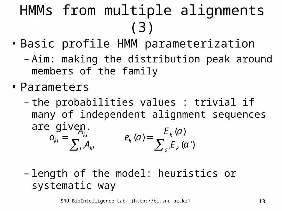
HMMs from multiple alignments (3)
• Basic profile HMM parameterization– Aim: making the distribution peak around
members of the family
• Parameters– the probabilities values : trivial if many of
independent alignment sequences are given.
– length of the model: heuristics or systematic way
'' ' )'(
)()(
a k
kk
l kl
klkl aE
aEae
A
Aa

SNU BioIntelligence Lab. (http://bi.snu.ac.kr) 14
HMMs from multiple alignments (4)
• Figure 5.4
SNU BioIntelligence Lab. (http://bi.snu.ac.kr) 15
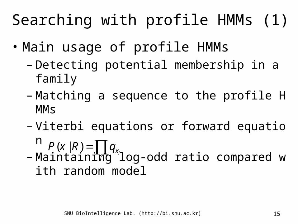
Searching with profile HMMs (1)
• Main usage of profile HMMs– Detecting potential membership in a family– Matching a sequence to the profile HMMs– Viterbi equations or forward equation– Maintaining log-odd ratio compared with random
model
i
xiqRxP )|(
SNU BioIntelligence Lab. (http://bi.snu.ac.kr) 16
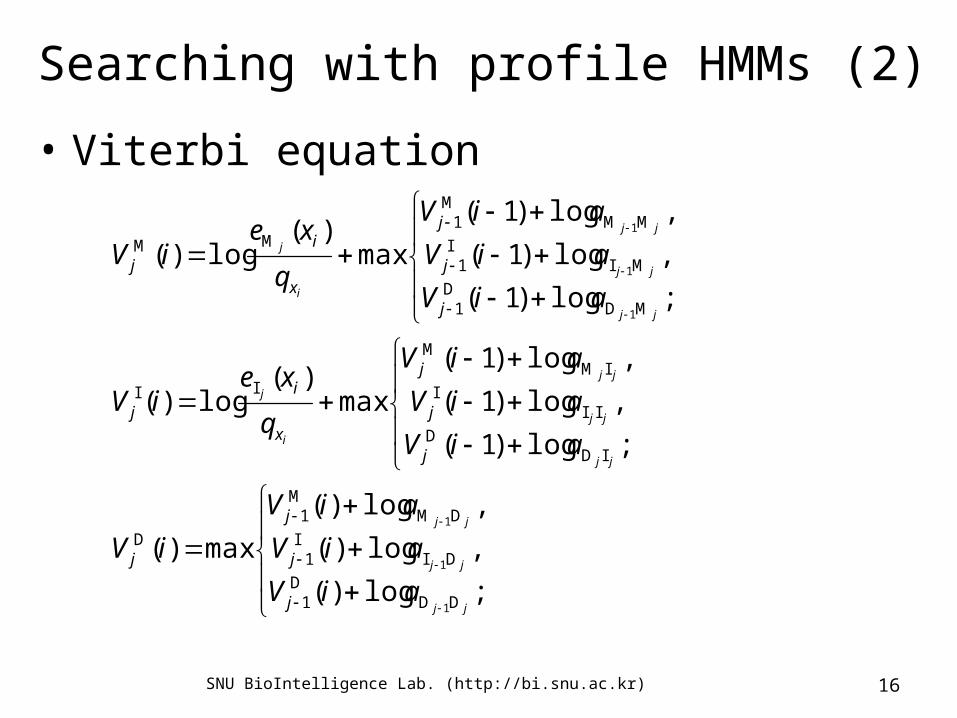
Searching with profile HMMs (2)
• Viterbi equation
;log)(
,log)(
,log)(
max)(
;log)1(
,log)1(
,log)1(
max)(
log)(
;log)1(
,log)1(
,log)1(
max)(
log)(
DDD
1
DII
1
DMM
1
D
IDD
III
IMM
II
MDD
1
MII
1
MMM
1MM
1
1
1
1
1
1
jj
jj
jj
jj
jj
jj
i
j
jj
jj
jj
i
j
aiV
aiV
aiV
iV
aiV
aiV
aiV
q
xeiV
aiV
aiV
aiV
q
xeiV
j
j
j
j
j
j
j
x
i
j
j
j
j
x
i
j
SNU BioIntelligence Lab. (http://bi.snu.ac.kr) 17
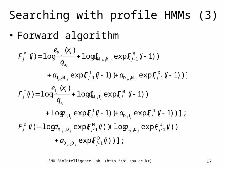
Searching with profile HMMs (3)
• Forward algorithm
))];(exp(
))(exp(log))(exp(log[)(
))];1(exp())1(exp(log
))1(exp(log[)(
log)(
))];1(exp())1(exp(
))1(exp(log[)(
log)(
D1DD
I1DI
M1DM
D
DID
III
MIM
II
D1MD
I1MI
M1MM
MM
1
11
11
1
iFa
iFaiFaiF
iFaiFa
iFaq
xeiF
iFaiFa
iFaq
xeiF
j
jjj
jj
jx
i
j
jj
jx
i
j
jj
jjjj
jjjj
jj
i
j
jjjj
jj
i
j
SNU BioIntelligence Lab. (http://bi.snu.ac.kr) 18
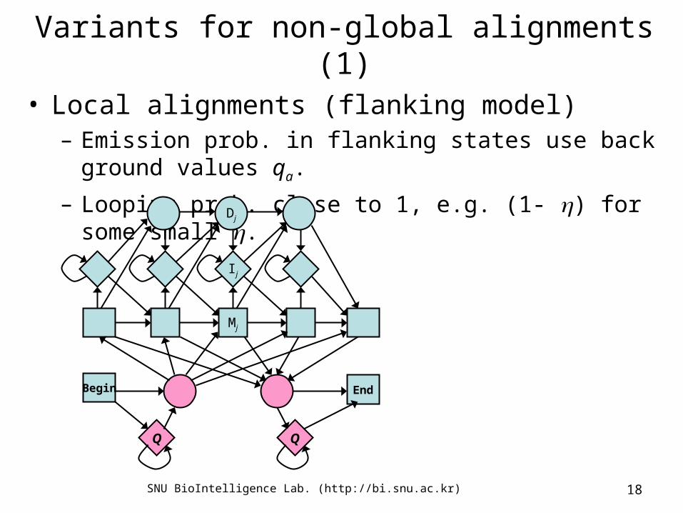
Variants for non-global alignments (1)
• Local alignments (flanking model)– Emission prob. in flanking states use background values q
a.– Looping prob. close to 1, e.g. (1- ) for some small .
Mj
Ij
Dj
Begin End
Q Q
SNU BioIntelligence Lab. (http://bi.snu.ac.kr) 19
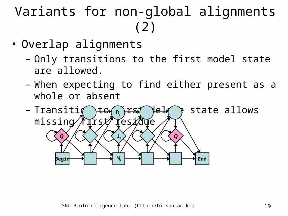
Variants for non-global alignments (2)
• Overlap alignments– Only transitions to the first model state are
allowed.– When expecting to find either present as a whole
or absent– Transition to first delete state allows missing first
residue
Begin Mj End
IjQ
Dj
Q
SNU BioIntelligence Lab. (http://bi.snu.ac.kr) 20
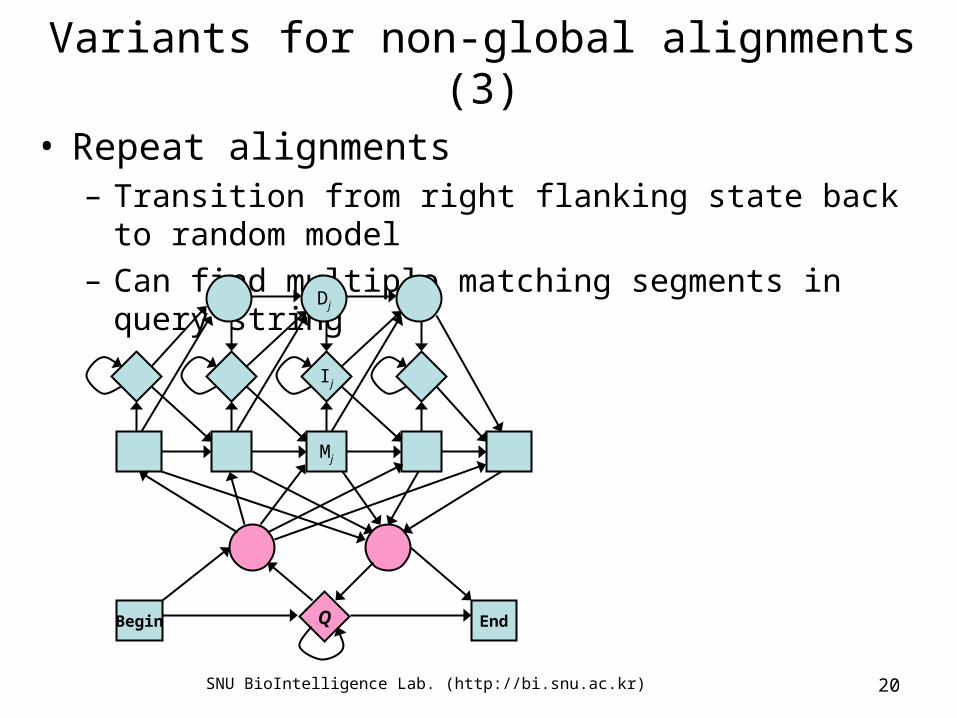
Variants for non-global alignments (3)
• Repeat alignments– Transition from right flanking state back to
random model– Can find multiple matching segments in query
string
Mj
Ij
Dj
Begin EndQ
SNU BioIntelligence Lab. (http://bi.snu.ac.kr) 21
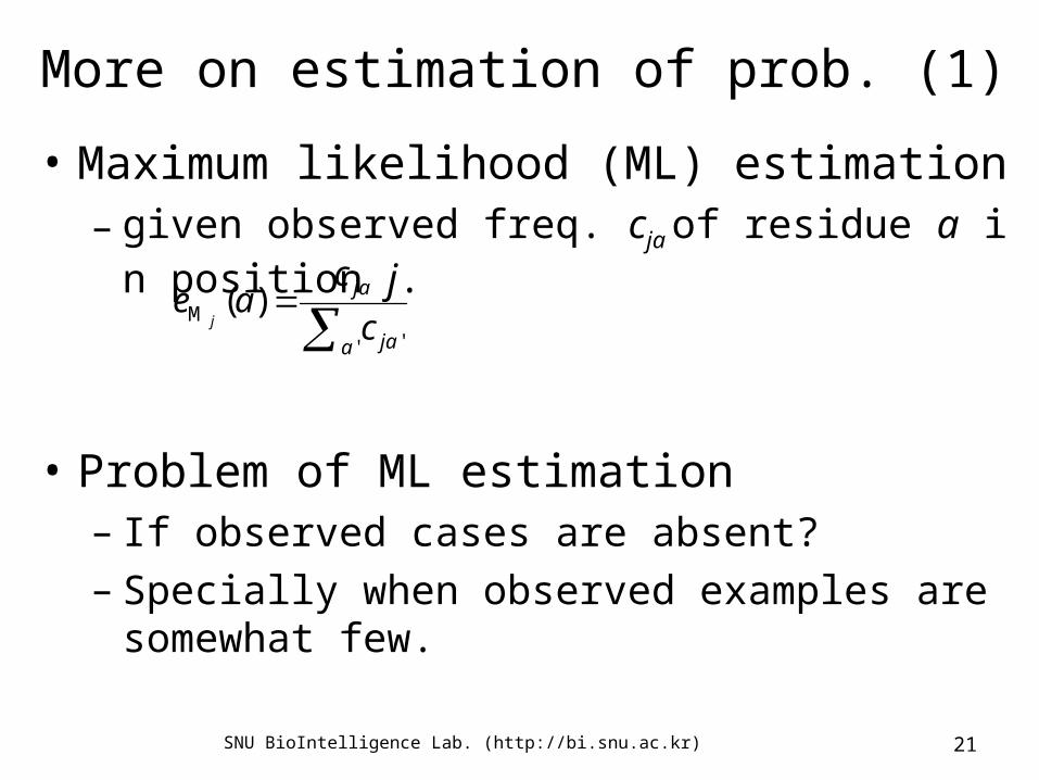
More on estimation of prob. (1)
• Maximum likelihood (ML) estimation– given observed freq. cja of residue a in position j.
• Problem of ML estimation– If observed cases are absent?– Specially when observed examples are somewhat
few.
' 'M )(
a ja
ja
c
cae
j

SNU BioIntelligence Lab. (http://bi.snu.ac.kr) 22
More on estimation of prob. (2)
• Simple pseudocounts– qa: background distribution– A: weight factor
– Laplace’s rule: Aqa = 1
• Bayesian framework– Dirichlet prior
' '
M )(a ja
aja
cA
Aqcae
j
)(
)()|()|(
DP
PDPDP
SNU BioIntelligence Lab. (http://bi.snu.ac.kr) 23
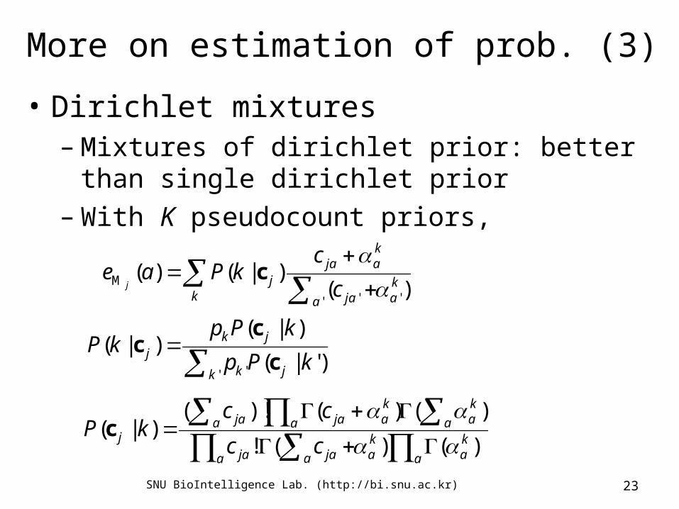
More on estimation of prob. (3)
• Dirichlet mixtures– Mixtures of dirichlet prior: better than single dirich
let prior– With K pseudocount priors,
)()|()(
'' 'M k
aa ja
kaja
kj c
ckPae
j
c
' ' )'|(
)|()|(
k jk
jkj kPp
kPpkP
c
cc
a
ka
kaa jaa ja
a
kaa
kajaa ja
j cc
cckP
)()(!
)()()!()|(
c
SNU BioIntelligence Lab. (http://bi.snu.ac.kr) 24
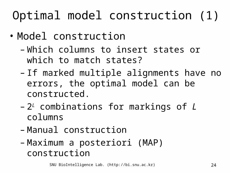
Optimal model construction (1)
• Model construction– Which columns to insert states or which to
match states?– If marked multiple alignments have no
errors, the optimal model can be constructed.
– 2L combinations for markings of L columns– Manual construction– Maximum a posteriori (MAP) construction
SNU BioIntelligence Lab. (http://bi.snu.ac.kr) 25
Optimal model construction (2)
beg M M M end
II II
D DD
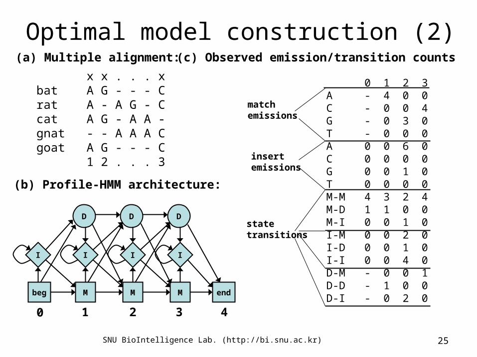
x x . . . xbat A G - - - Crat A - A G - Ccat A G - A A -gnat - - A A A Cgoat A G - - - C 1 2 . . . 3
(a) Multiple alignment:
(b) Profile-HMM architecture:
0 1 2 3 4
0 1 2 3A - 4 0 0C - 0 0 4G - 0 3 0T - 0 0 0A 0 0 6 0C 0 0 0 0G 0 0 1 0T 0 0 0 0M-M 4 3 2 4M-D 1 1 0 0M-I 0 0 1 0I-M 0 0 2 0I-D 0 0 1 0I-I 0 0 4 0D-M - 0 0 1D-D - 1 0 0D-I - 0 2 0
(c) Observed emission/transition counts
matchemissions
insertemissions
statetransitions
SNU BioIntelligence Lab. (http://bi.snu.ac.kr) 26
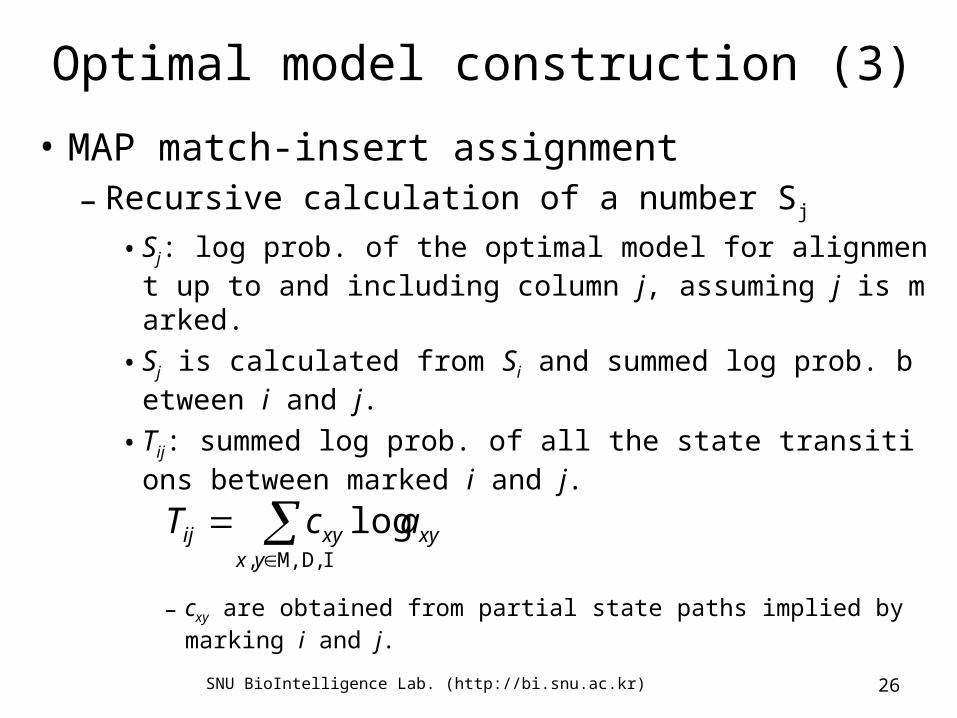
Optimal model construction (3)
• MAP match-insert assignment– Recursive calculation of a number Sj
• Sj: log prob. of the optimal model for alignment up to and including column j, assuming j is marked.
• Sj is calculated from Si and summed log prob. between i and j.
• Tij: summed log prob. of all the state transitions between marked i and j.
– cxy are obtained from partial state paths implied by marking i and j.
ID,M,,
logyx
xyxyij acT
SNU BioIntelligence Lab. (http://bi.snu.ac.kr) 27
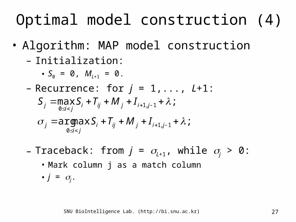
Optimal model construction (4)
• Algorithm: MAP model construction– Initialization:
• S0 = 0, ML+1 = 0.
– Recurrence: for j = 1,..., L+1:
– Traceback: from j = L+1, while j > 0:• Mark column j as a match column• j = j.
;maxarg
;max
1,10
1,10
jijijiji
j
jijijiji
j
IMTS
IMTSS

SNU BioIntelligence Lab. (http://bi.snu.ac.kr) 28
Weighting training sequences (1)
• Good random sample do you have?• “Assumption : all examples are
independent samples” might be incorrect
• Solutions– Weight sequences based on similarity

SNU BioIntelligence Lab. (http://bi.snu.ac.kr) 29
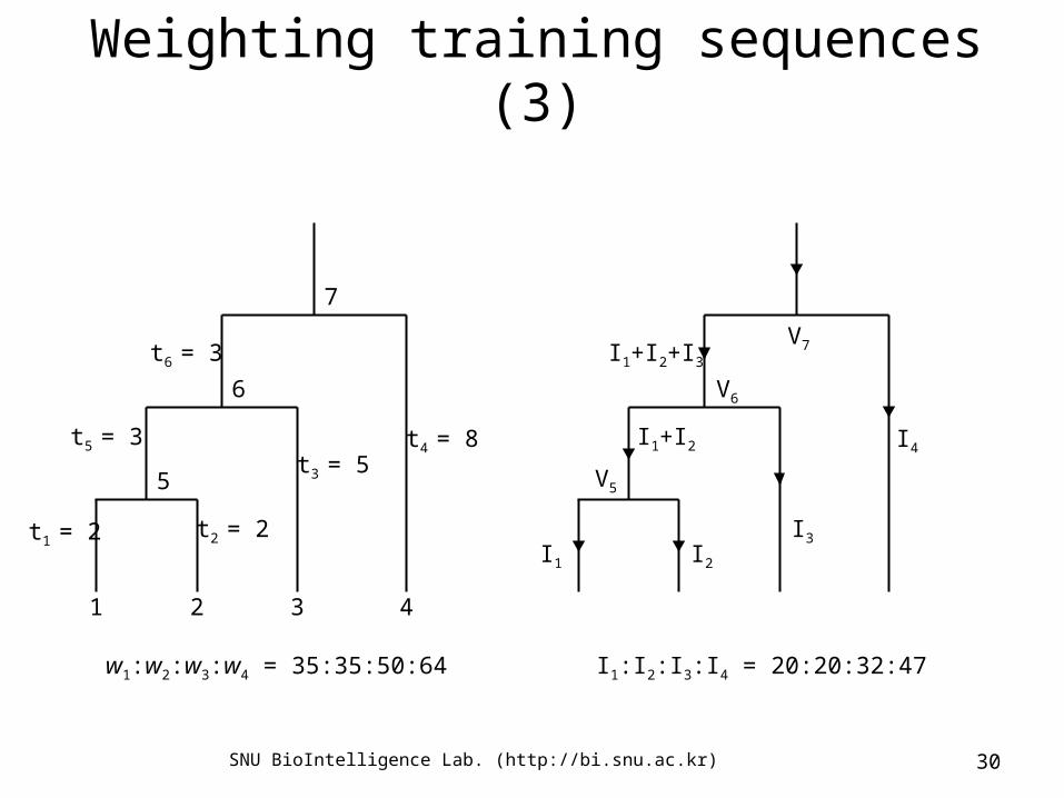
Weighting training sequences (2)
• Simple weighting schemes derived from a tree– Phylogenetic tree is given.
• [Thompson, Higgins & Gibson 1994b]– Kirchohoff’s law
• [Gerstein, Sonnhammer & Chothia 1994]
nk k
ini w
wtw
below leaves
SNU BioIntelligence Lab. (http://bi.snu.ac.kr) 30
Weighting training sequences (3)
t4 = 8t3 = 5
t2 = 2t1 = 2
t5 = 3
t6 = 3
5
6
7
1 2 3 4
I4I1+I2
I1+I2+I3
V5
V6
V7
I1 I2
I3
I1:I2:I3:I4 = 20:20:32:47w1:w2:w3:w4 = 35:35:50:64
SNU BioIntelligence Lab. (http://bi.snu.ac.kr) 31
Weighting training sequences (4)
• Root weights from Gaussian parameters– Influence of leaves on the root distr.– Altchul-Carroll-Lipman wieghts
• Make gaussian distr.• Mean : linearly combination of xi.• Combination weights represent the influences of leave
s.

SNU BioIntelligence Lab. (http://bi.snu.ac.kr) 32
Weighting training sequences (5)
t3
t2t1
4
x1 x2 x3
5
12
22211
2
)(
121 ),|4 nodeat ( t
xvxvx
eKLLxP
2211
21211221112121 )/(),/(),/(
xvxv
ttttttttvtttv
SNU BioIntelligence Lab. (http://bi.snu.ac.kr) 33
Weighting training sequences (6)
• Voronoi weights– Proportional to the volume of empty space– Sequence family in sequence space– Algorithm
• Random sample: choosing at kth position uniformly from the set of residues occurring kth position
• ni: count of samples closest to the ith family• ith weight
k ki nn /
SNU BioIntelligence Lab. (http://bi.snu.ac.kr) 34
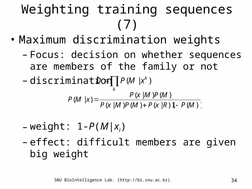
Weighting training sequences (7)
• Maximum discrimination weights– Focus: decision on whether sequences are
members of the family or not– discrimination
– weight: 1-P(M|xi)
– effect: difficult members are given big weight
k
kxMPD )|(
))(1)(|()()|(
)()|()|(
MPRxPMPMxP
MPMxPxMP
SNU BioIntelligence Lab. (http://bi.snu.ac.kr) 35
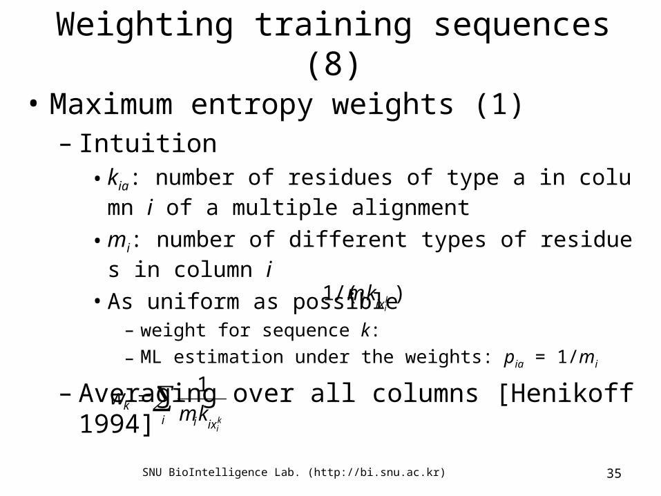
Weighting training sequences (8)
• Maximum entropy weights (1)– Intuition
• kia: number of residues of type a in column i of a multiple alignment
• mi: number of different types of residues in column i• As uniform as possible
– weight for sequence k:– ML estimation under the weights: pia = 1/mi
– Averaging over all columns [Henikoff 1994]
)/(1 kiixikm
i ixi
kki
kmw
1
SNU BioIntelligence Lab. (http://bi.snu.ac.kr) 36
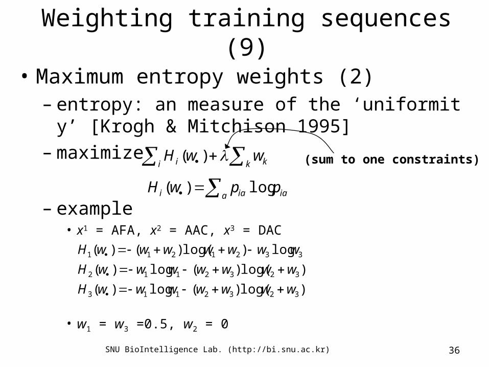
Weighting training sequences (9)
• Maximum entropy weights (2)– entropy: an measure of the ‘uniformity’ [Krogh &
Mitchison 1995]– maximize
– example• x1 = AFA, x2 = AAC, x3 = DAC
• w1 = w3 =0.5, w2 = 0
k ki i wwH )(
iaa iai ppwH log)(
(sum to one constraints)
)log()(log)(
)log()(log)(
log)log()()(
3232113
3232112
3321211
wwwwwwwH
wwwwwwwH
wwwwwwwH