1

Chapter 3. Occupational Employment Statistics

(Last updated December 2008) The Occupational Employment Statistics (OES) survey is a mail survey measuring occupational

employment and wage rates of wage and salary workers in nonfarm establishments in the 50

States and the District of Columbia. Guam, Puerto Rico, and the Virgin Islands are also

surveyed, but their data are not included in national estimates.

About 6.8 million in-scope establishments are stratified within their respective States by

substate area and industry. Substate areas include all officially defined metropolitan areas and

one or more residual balance-of-State areas (MSA/BOS areas). The North American Industry

Classification System (NAICS) is used to stratify establishments by industry.

The U.S. Bureau of Labor Statistics selects semiannual probability samples—referred to

as panels—of about 200,000 business establishments. Responses are obtained through mail,

telephone contact, and e-mail or other electronic means. Most respondents report their number of

employees by occupation across 12 wage bands. Currently, there are 97 different survey forms—

each used for a different set of industries—as well as a write-in form sent to the smallest

establishments. The Standard Occupational Classification (SOC) system is used to define

occupations.

Estimates of occupational employment and occupational wage rates are based on a rolling

six-panel (or 3-year) cycle. The final in-scope post-collection sample size when six panels are

combined is approximately 1.1 million establishments.

Background

In 1971, questionnaires were sent to 50,000 manufacturing establishments throughout the United

States, marking the beginning of the OES survey. This survey was conducted in cooperation with

the Employment and Training Administration and 15 State Workforce Agencies (SWAs). It was

designed to obtain national and State occupational employment estimates for the cooperating

States. Following the completion of the manufacturing survey, similar surveys were developed

for nonmanufacturing industries and State and local governments.

2

From 1988 to 1995, a new OES data collection method began with the compilation of

employment data by industry in a 3-year cycle. These data do not include wage information, data

by State or metropolitan area, or cross-industry data. Rather, they consist of industry-based

employment estimates by 2-digit and 3-digit Standard Industrial Classification (SIC) industry.

Each industry was surveyed once every 3 years. As a result, the 1988–1995 estimates are useful

mainly to data users interested in occupational staffing patterns for specific industries during this

period. Note that OES estimates are not available before 1988 or for the year 1996.

For the year 1996 the OES program began collecting occupational wage data, in addition to

occupational employment data, for every State. In addition, the program's 3-year survey cycle

was modified to collect data from all covered industries each year. In 1997 the OES program

began producing both industry-specific and cross-industry estimates of occupational employment

and wages. From 1997-2002, OES data from 400,000 establishments were collected annually

using an October, November, or December payroll reference period.

In 1999, the OES survey began using the U.S. Office of Management and Budget’s

(OMB) new occupational classification system—the Standard Occupational Classification (SOC)

system. (See http://www.bls.gov/soc/home.htm for information on the SOC system.) The SOC is

the first OMB-required occupational classification system for Federal statistical agencies. The

OES survey uses 22 major occupational groups from the SOC to categorize workers into 1 of

801 detailed occupations.

In 2002, the OES survey switched from the Standard Industrial Classification (SIC) system to the

North American Industry Classification System (NAICS). More information about NAICS can

be found at the BLS Web site http://www.bls.gov/bls/naics.htm or in the 2002 North American

Industry Classification System manual. Each establishment is assigned a 6-digit NAICS code

based on its primary activity. Also, starting with the 2002 survey, OES began collecting data

from 200,000 establishments semiannually using May and November reference periods.

Industrial scope and stratification

3

The survey covers the following NAICS industry sectors:

11 Logging (1133), support activities for crop production

(1151), and support activities for animal production (1152) only

21 Mining

22 Utilities

23 Construction

31-33 Manufacturing

42 Wholesale Trade

44-45 Retail Trade

48-49 Transportation and warehousing

51 Information

52 Finance and insurance

53 Real estate and rental and leasing

54 Professional, scientific, and technical services

55 Management of companies and enterprises

56 Administrative and support and waste management and

remediation services

61 Educational services

62 Health care and social assistance

71 Arts, entertainment, and recreation

72 Accommodation and food services

81 Other services, except public administration [private

households (814) are excluded]

99 Federal, State, and local government (OES designation)

These sectors are stratified into about 340 industry groups at the 4- or 5-digit NAICS level. Industry stratification is mostly at the 4-digit level. However, some 5-digit groups are used because of the heterogeneity of the 4-digit groups and the unique occupations found among the 5-digit industries.

4

Concepts

Establishment- An establishment is a single physical location at which economic activity occurs

(e.g., a store, a factory, a restaurant, etc.). Each establishment is assigned a six-digit NAICS

code. When a single physical location encompasses two or more distinct economic activities, it is

treated as two or more separate establishments if separate payroll records are available and

certain other criteria are met.

Employment- Employment refers to the number of workers who can be classified as full- or part-

time employees, including workers on paid vacations or other types of leave; salaried officers,

executives, and staff members of incorporated firms; employees temporarily assigned to other

units; and non-contract employees for whom the reporting unit is the permanent duty station,

regardless of whether that unit prepares their paychecks.

Occupations- Workers are classified into occupations on the basis of the work performed and the

skills required in each occupation. Employees are assigned to an occupation on the basis of the

work they perform and not on the basis of their education or training. For example, an employee

trained as an engineer but working as a drafter is reported as a drafter. An employee who

performs the duties of two or more occupations is reported in the occupation that requires the

highest level of skill or in the occupation in which the employee spends the most time if there is

no measurable difference in skill requirements. Working supervisors (those spending 20 percent

or more of their time doing work similar to the workers they supervise) are classified with the

workers they supervise. Workers receiving on-the-job training, apprentices, and trainees are

classified in the occupations for which they are being trained.

A wage is money that is paid or received for work or services performed in a specified period.

Base rate pay, cost-of-living allowances, guaranteed pay, hazardous-duty pay, incentive pay such

as commissions and production bonuses, tips, and on-call pay are included in a wage. Back pay,

jury duty pay, overtime pay, severance pay, shift differentials, nonproduction bonuses, employer

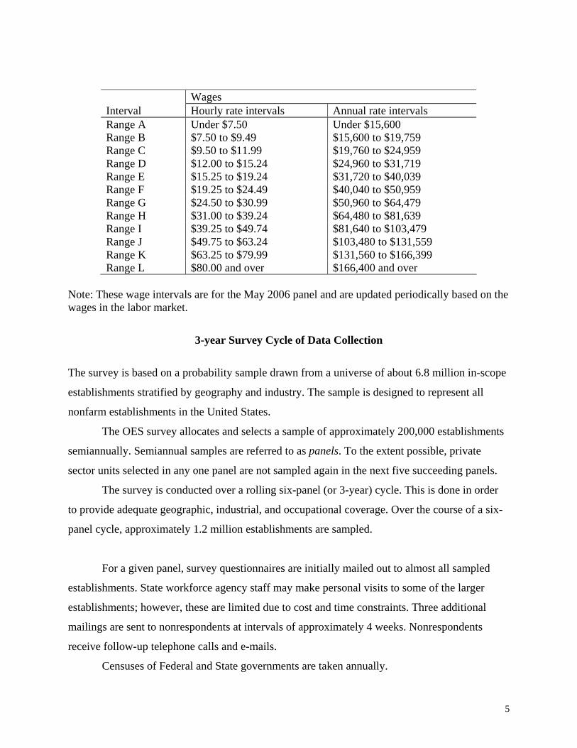
costs for supplementary benefits, and tuition reimbursements are excluded. Employers are asked

to classify each of their workers into an SOC occupation and one of the following 12 wage

intervals:

5

Wages Interval Hourly rate intervals Annual rate intervals Range A Under $7.50 Under $15,600 Range B $7.50 to $9.49 $15,600 to $19,759 Range C $9.50 to $11.99 $19,760 to $24,959 Range D $12.00 to $15.24 $24,960 to $31,719 Range E $15.25 to $19.24 $31,720 to $40,039 Range F $19.25 to $24.49 $40,040 to $50,959 Range G $24.50 to $30.99 $50,960 to $64,479 Range H $31.00 to $39.24 $64,480 to $81,639 Range I $39.25 to $49.74 $81,640 to $103,479 Range J $49.75 to $63.24 $103,480 to $131,559 Range K $63.25 to $79.99 $131,560 to $166,399 Range L $80.00 and over $166,400 and over

Note: These wage intervals are for the May 2006 panel and are updated periodically based on the wages in the labor market.

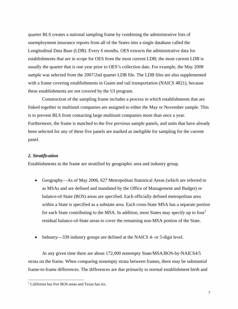
3-year Survey Cycle of Data Collection

The survey is based on a probability sample drawn from a universe of about 6.8 million in-scope

establishments stratified by geography and industry. The sample is designed to represent all

nonfarm establishments in the United States.

The OES survey allocates and selects a sample of approximately 200,000 establishments

semiannually. Semiannual samples are referred to as panels. To the extent possible, private

sector units selected in any one panel are not sampled again in the next five succeeding panels.

The survey is conducted over a rolling six-panel (or 3-year) cycle. This is done in order

to provide adequate geographic, industrial, and occupational coverage. Over the course of a six-

panel cycle, approximately 1.2 million establishments are sampled.

For a given panel, survey questionnaires are initially mailed out to almost all sampled

establishments. State workforce agency staff may make personal visits to some of the larger

establishments; however, these are limited due to cost and time constraints. Three additional

mailings are sent to nonrespondents at intervals of approximately 4 weeks. Nonrespondents

receive follow-up telephone calls and e-mails.

Censuses of Federal and State governments are taken annually.

6

• Through administrative records, the U.S. Office of Personnel Management and U.S.

Postal Service provide complete enumeration of Federal executive branch and postal

service employment annually for a June reference month. BLS processes employment

and wage information from these files. Data from only the most recent year are retained

for use in OES estimates.

• Every November, for each area, State governments provide a census of employment at

establishments, except for schools and hospitals. Data from only the most recent year are

retained for use in OES estimates.

• A probability sample is taken of local government establishments, except for hospitals, in

every State except Hawaii.

• A census of Hawaii’s local government is conducted annually each November. With the

exception of schools and hospitals, all local-government-owned establishments in Hawaii

are included.

• A census of public- and private-owned hospitals is taken over the 3-year period.

• A probability sample of schools owned by State or local government, as well as schools

in the private sector, is taken over the 3-year period.

Sampling Procedures

The five steps

The creation of the OES sample consists of five steps:

1. Frame Construction

The sampling frame, or universe, is a list of about 6.8 million in-scope nonfarm establishments

that file unemployment insurance (UI) reports to the State workforce agencies. Employers are

required by law to file these reports to the State where each establishment is located. Every

7

quarter BLS creates a national sampling frame by combining the administrative lists of

unemployment insurance reports from all of the States into a single database called the

Longitudinal Data Base (LDB). Every 6 months, OES extracts the administrative data for

establishments that are in scope for OES from the most current LDB; the most current LDB is

usually the quarter that is one year prior to OES’s collection date. For example, the May 2008

sample was selected from the 2007/2nd quarter LDB file. The LDB files are also supplemented

with a frame covering establishments in Guam and rail transportation (NAICS 4821), because

these establishments are not covered by the UI program.

Construction of the sampling frame includes a process in which establishments that are

linked together in multiunit companies are assigned to either the May or November sample. This

is to prevent BLS from contacting large multiunit companies more than once a year.

Furthermore, the frame is matched to the five previous sample panels, and units that have already

been selected for any of these five panels are marked as ineligible for sampling for the current

panel.

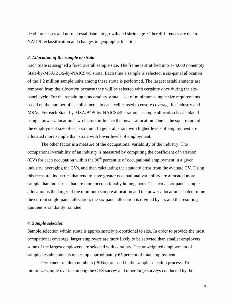
2. Stratification

Establishments in the frame are stratified by geographic area and industry group.

• Geography—As of May 2006, 627 Metropolitan Statistical Areas (which are referred to

as MSAs and are defined and mandated by the Office of Management and Budget) or

balance-of-State (BOS) areas are specified. Each officially defined metropolitan area

within a State is specified as a substate area. Each cross-State MSA has a separate portion

for each State contributing to the MSA. In addition, most States may specify up to four1

residual balance-of-State areas to cover the remaining non-MSA portion of the State.

• Industry—339 industry groups are defined at the NAICS 4- or 5-digit level.

At any given time there are about 172,000 nonempty State/MSA/BOS-by-NAICS4/5

strata on the frame. When comparing nonempty strata between frames, there may be substantial

frame-to-frame differences. The differences are due primarily to normal establishment birth and

1 California has five BOS areas and Texas has six.

8

death processes and normal establishment growth and shrinkage. Other differences are due to

NAICS reclassification and changes in geographic location.

3. Allocation of the sample to strata

Each State is assigned a fixed overall sample size. The frame is stratified into 174,000 nonempty

State-by-MSA/BOS-by-NAICS4/5 strata. Each time a sample is selected, a six-panel allocation

of the 1.2 million sample units among these strata is performed. The largest establishments are

removed from the allocation because they will be selected with certainty once during the six-

panel cycle. For the remaining noncertainty strata, a set of minimum sample size requirements

based on the number of establishments in each cell is used to ensure coverage for industry and

MSAs. For each State-by-MSA/BOS-by-NAICS4/5 stratum, a sample allocation is calculated

using a power allocation. Two factors influence the power allocation. One is the square root of

the employment size of each stratum. In general, strata with higher levels of employment are

allocated more sample than strata with lower levels of employment.

The other factor is a measure of the occupational variability of the industry. The

occupational variability of an industry is measured by computing the coefficient of variation

(CV) for each occupation within the 90th percentile of occupational employment in a given

industry, averaging the CVs, and then calculating the standard error from the average CV. Using

this measure, industries that tend to have greater occupational variability are allocated more

sample than industries that are more occupationally homogenous. The actual six-panel sample

allocation is the larger of the minimum sample allocation and the power allocation. To determine

the current single-panel allocation, the six-panel allocation is divided by six and the resulting

quotient is randomly rounded.

4. Sample selection

Sample selection within strata is approximately proportional to size. In order to provide the most

occupational coverage, larger employers are more likely to be selected than smaller employers;

some of the largest employers are selected with certainty. The unweighted employment of

sampled establishments makes up approximately 65 percent of total employment.

Permanent random numbers (PRNs) are used in the sample selection process. To

minimize sample overlap among the OES survey and other large surveys conducted by the

9

Bureau of Labor Statistics, each establishment is assigned a PRN. For each stratum, a specific

PRN value is designated as the “starting point” to select a sample. From this starting point, we

sequentially select the first n eligible establishments in the frame into the sample where n

denotes the number of establishments to be sampled.

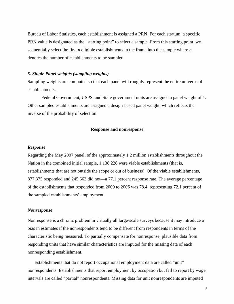
5. Single Panel weights (sampling weights)

Sampling weights are computed so that each panel will roughly represent the entire universe of

establishments.

Federal Government, USPS, and State government units are assigned a panel weight of 1.

Other sampled establishments are assigned a design-based panel weight, which reflects the

inverse of the probability of selection.

Response and nonresponse

Response

Regarding the May 2007 panel, of the approximately 1.2 million establishments throughout the

Nation in the combined initial sample, 1,138,228 were viable establishments (that is,

establishments that are not outside the scope or out of business). Of the viable establishments,

877,375 responded and 245,663 did not—a 77.1 percent response rate. The average percentage

of the establishments that responded from 2000 to 2006 was 78.4, representing 72.1 percent of

the sampled establishments’ employment.

Nonresponse

Nonresponse is a chronic problem in virtually all large-scale surveys because it may introduce a

bias in estimates if the nonrespondents tend to be different from respondents in terms of the

characteristic being measured. To partially compensate for nonresponse, plausible data from

responding units that have similar characteristics are imputed for the missing data of each

nonresponding establishment.

Establishments that do not report occupational employment data are called “unit”

nonrespondents. Establishments that report employment by occupation but fail to report by wage

intervals are called “partial” nonrespondents. Missing data for unit nonrespondents are imputed

10

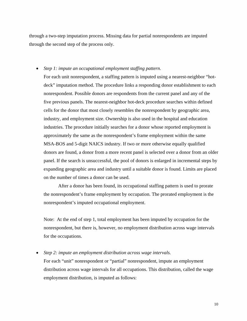
through a two-step imputation process. Missing data for partial nonrespondents are imputed

through the second step of the process only.

• Step 1: impute an occupational employment staffing pattern.

For each unit nonrespondent, a staffing pattern is imputed using a nearest-neighbor “hot-

deck” imputation method. The procedure links a responding donor establishment to each

nonrespondent. Possible donors are respondents from the current panel and any of the

five previous panels. The nearest-neighbor hot-deck procedure searches within defined

cells for the donor that most closely resembles the nonrespondent by geographic area,

industry, and employment size. Ownership is also used in the hospital and education

industries. The procedure initially searches for a donor whose reported employment is

approximately the same as the nonrespondent’s frame employment within the same

MSA-BOS and 5-digit NAICS industry. If two or more otherwise equally qualified

donors are found, a donor from a more recent panel is selected over a donor from an older

panel. If the search is unsuccessful, the pool of donors is enlarged in incremental steps by

expanding geographic area and industry until a suitable donor is found. Limits are placed

on the number of times a donor can be used.

After a donor has been found, its occupational staffing pattern is used to prorate

the nonrespondent’s frame employment by occupation. The prorated employment is the

nonrespondent’s imputed occupational employment.

Note: At the end of step 1, total employment has been imputed by occupation for the

nonrespondent, but there is, however, no employment distribution across wage intervals

for the occupations.

• Step 2: impute an employment distribution across wage intervals.

For each “unit” nonrespondent or “partial” nonrespondent, impute an employment

distribution across wage intervals for all occupations. This distribution, called the wage

employment distribution, is imputed as follows:

11

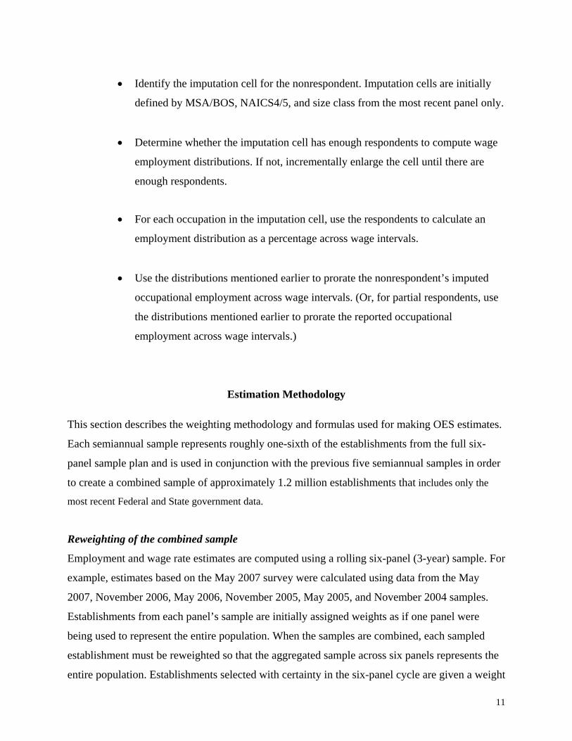
• Identify the imputation cell for the nonrespondent. Imputation cells are initially

defined by MSA/BOS, NAICS4/5, and size class from the most recent panel only.

• Determine whether the imputation cell has enough respondents to compute wage

employment distributions. If not, incrementally enlarge the cell until there are

enough respondents.

• For each occupation in the imputation cell, use the respondents to calculate an

employment distribution as a percentage across wage intervals.

• Use the distributions mentioned earlier to prorate the nonrespondent’s imputed

occupational employment across wage intervals. (Or, for partial respondents, use

the distributions mentioned earlier to prorate the reported occupational

employment across wage intervals.)

Estimation Methodology This section describes the weighting methodology and formulas used for making OES estimates.

Each semiannual sample represents roughly one-sixth of the establishments from the full six-

panel sample plan and is used in conjunction with the previous five semiannual samples in order

to create a combined sample of approximately 1.2 million establishments that includes only the

most recent Federal and State government data.

Reweighting of the combined sample

Employment and wage rate estimates are computed using a rolling six-panel (3-year) sample. For

example, estimates based on the May 2007 survey were calculated using data from the May

2007, November 2006, May 2006, November 2005, May 2005, and November 2004 samples.

Establishments from each panel’s sample are initially assigned weights as if one panel were

being used to represent the entire population. When the samples are combined, each sampled

establishment must be reweighted so that the aggregated sample across six panels represents the

entire population. Establishments selected with certainty in the six-panel cycle are given a weight

12

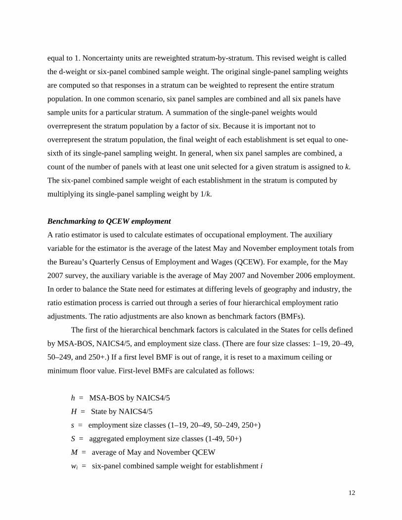
equal to 1. Noncertainty units are reweighted stratum-by-stratum. This revised weight is called

the d-weight or six-panel combined sample weight. The original single-panel sampling weights

are computed so that responses in a stratum can be weighted to represent the entire stratum

population. In one common scenario, six panel samples are combined and all six panels have

sample units for a particular stratum. A summation of the single-panel weights would

overrepresent the stratum population by a factor of six. Because it is important not to

overrepresent the stratum population, the final weight of each establishment is set equal to one-

sixth of its single-panel sampling weight. In general, when six panel samples are combined, a

count of the number of panels with at least one unit selected for a given stratum is assigned to k.

The six-panel combined sample weight of each establishment in the stratum is computed by

multiplying its single-panel sampling weight by 1/k.

Benchmarking to QCEW employment

A ratio estimator is used to calculate estimates of occupational employment. The auxiliary

variable for the estimator is the average of the latest May and November employment totals from

the Bureau’s Quarterly Census of Employment and Wages (QCEW). For example, for the May

2007 survey, the auxiliary variable is the average of May 2007 and November 2006 employment.

In order to balance the State need for estimates at differing levels of geography and industry, the

ratio estimation process is carried out through a series of four hierarchical employment ratio

adjustments. The ratio adjustments are also known as benchmark factors (BMFs).

The first of the hierarchical benchmark factors is calculated in the States for cells defined

by MSA-BOS, NAICS4/5, and employment size class. (There are four size classes: 1–19, 20–49,

50–249, and 250+.) If a first level BMF is out of range, it is reset to a maximum ceiling or

minimum floor value. First-level BMFs are calculated as follows:

h = MSA-BOS by NAICS4/5

H = State by NAICS4/5

s = employment size classes (1–19, 20–49, 50–249, 250+)

S = aggregated employment size classes (1-49, 50+)

M = average of May and November QCEW

wi = six-panel combined sample weight for establishment i

13

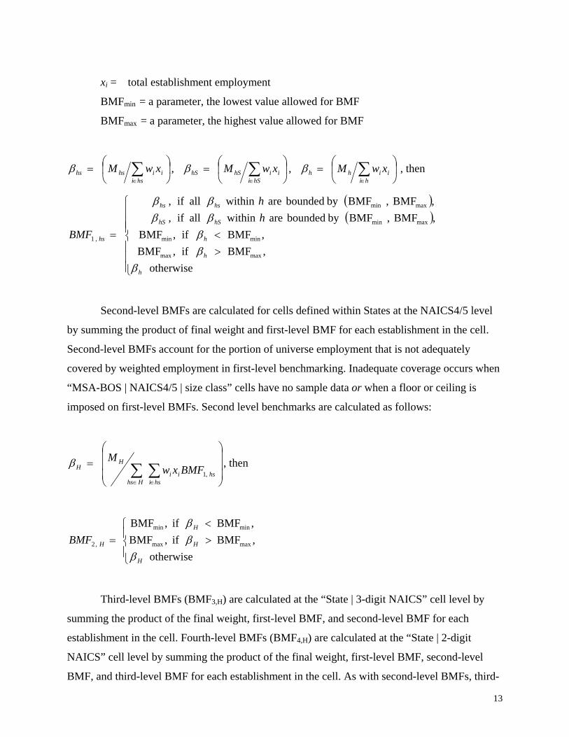
xi = total establishment employment

BMFmin = a parameter, the lowest value allowed for BMF

BMFmax = a parameter, the highest value allowed for BMF

⎟⎠

⎞⎜⎝

⎛= ∑∈hsi

iihshs xwMβ , ⎟⎠

⎞⎜⎝

⎛= ∑∈hSi

iihShS xwMβ , ⎟⎠

⎞⎜⎝

⎛= ∑∈hi

iihh xwMβ , then

( )( )

⎪⎪⎪

⎩

⎪⎪⎪

⎨

⎧

><=

otherwise,BMFif,BMF,BMFif,BMF

,BMF,BMFby boundedarewithinallif,,BMF,BMFby boundedarewithinallif,

maxmax

minmin

maxmin

maxmin

,1

h

h

h

hShS

hshs

hs

hh

BMF

βββββββ

Second-level BMFs are calculated for cells defined within States at the NAICS4/5 level

by summing the product of final weight and first-level BMF for each establishment in the cell.

Second-level BMFs account for the portion of universe employment that is not adequately

covered by weighted employment in first-level benchmarking. Inadequate coverage occurs when

“MSA-BOS | NAICS4/5 | size class” cells have no sample data or when a floor or ceiling is

imposed on first-level BMFs. Second level benchmarks are calculated as follows:

⎟⎟⎟

⎠

⎞

⎜⎜⎜

⎝

⎛= ∑ ∑

∈ ∈Hhs hsihsii

HH BMFxw

M,1

β , then

⎪⎩

⎪⎨

⎧><

=otherwise

,BMFif,BMF,BMFif,BMF

maxmax

minmin

,2

H

H

H

HBMFβ

ββ

Third-level BMFs (BMF3,H) are calculated at the “State | 3-digit NAICS” cell level by

summing the product of the final weight, first-level BMF, and second-level BMF for each

establishment in the cell. Fourth-level BMFs (BMF4,H) are calculated at the “State | 2-digit

NAICS” cell level by summing the product of the final weight, first-level BMF, second-level

BMF, and third-level BMF for each establishment in the cell. As with second-level BMFs, third-

14

and fourth-level BMFs are computed to account for inadequate coverage of the universe

employment.

A final benchmark factor, BMFi, is calculated for each establishment as the product of its

four hierarchical benchmark factors (BMFi = BMF1 * BMF2 * BMF3 * BMF4). A benchmark

weight value is then calculated as the product of the establishment’s six-panel combined sample

weight and final benchmark factor.

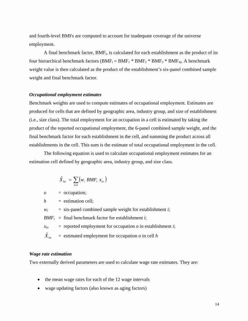
Occupational employment estimates

Benchmark weights are used to compute estimates of occupational employment. Estimates are

produced for cells that are defined by geographic area, industry group, and size of establishment

(i.e., size class). The total employment for an occupation in a cell is estimated by taking the

product of the reported occupational employment, the 6-panel combined sample weight, and the

final benchmark factor for each establishment in the cell, and summing the product across all

establishments in the cell. This sum is the estimate of total occupational employment in the cell.

The following equation is used to calculate occupational employment estimates for an

estimation cell defined by geographic area, industry group, and size class.

( )∑∈

=hi

ioiiho xBMFwX

o = occupation;

h = estimation cell;

wi = six-panel combined sample weight for establishment i;

BMFi = final benchmark factor for establishment i;

xio = reported employment for occupation o in establishment i;

hoX = estimated employment for occupation o in cell h

Wage rate estimation

Two externally derived parameters are used to calculate wage rate estimates. They are:

• the mean wage rates for each of the 12 wage intervals

• wage updating factors (also known as aging factors)

15

Wage rates of workers are reported to the OES survey as grouped data across 12

consecutive, nonoverlapping wage bands. Individual wage rates are not collected.

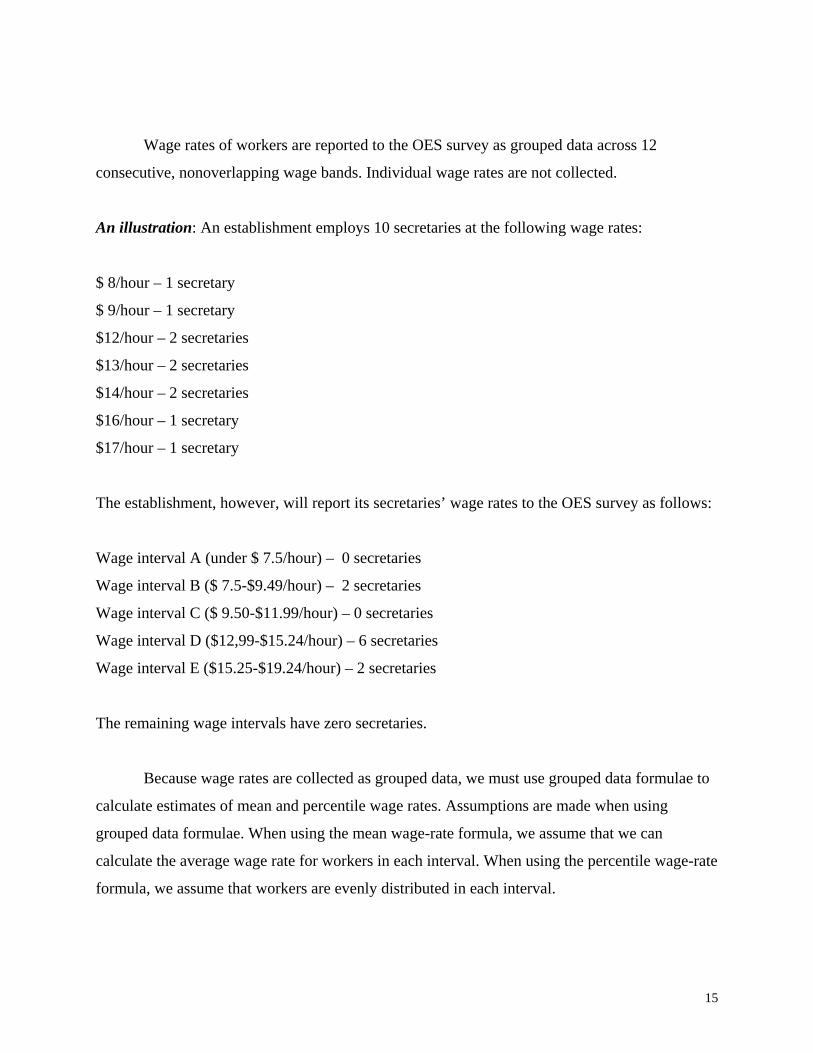
An illustration: An establishment employs 10 secretaries at the following wage rates:

$ 8/hour – 1 secretary

$ 9/hour – 1 secretary

$12/hour – 2 secretaries

$13/hour – 2 secretaries

$14/hour – 2 secretaries

$16/hour – 1 secretary

$17/hour – 1 secretary

The establishment, however, will report its secretaries’ wage rates to the OES survey as follows:

Wage interval A (under $ 7.5/hour) – 0 secretaries

Wage interval B ($ 7.5-$9.49/hour) – 2 secretaries

Wage interval C ($ 9.50-$11.99/hour) – 0 secretaries

Wage interval D ($12,99-$15.24/hour) – 6 secretaries

Wage interval E ($15.25-$19.24/hour) – 2 secretaries

The remaining wage intervals have zero secretaries.

Because wage rates are collected as grouped data, we must use grouped data formulae to

calculate estimates of mean and percentile wage rates. Assumptions are made when using

grouped data formulae. When using the mean wage-rate formula, we assume that we can

calculate the average wage rate for workers in each interval. When using the percentile wage-rate

formula, we assume that workers are evenly distributed in each interval.

16

Wage data from different panels are not equivalent in real-dollar terms because of

inflation and rising living costs. Consequently, wage data collected prior to the current survey

reference period have to be updated or aged to approximate that period.

Determining a mean wage rate for each interval

The mean hourly wage rate for all workers in any given wage interval is not computed using

grouped data collected by the OES survey. Rather, this value is calculated externally using data

from the Bureau’s National Compensation Survey (NCS). Although smaller than the OES survey

in terms of sample size, the NCS program, unlike OES, collects individual wage data. The mean

hourly wage rate for interval L (the upper, open-ended wage interval) is calculated without wage

data for pilots. This occupation is excluded because pilots work fewer hours than workers in

other occupations. Consequently, their hourly wage rates are much higher.

Wage aging process

Aging factors are developed from the Bureau’s Employment Cost Index (ECI) survey. The ECI

survey measures the rate of change in compensation for eleven major occupational groups on a

quarterly basis. Aging factors are used to adjust OES wage data from past survey reference

periods to the current survey reference period.

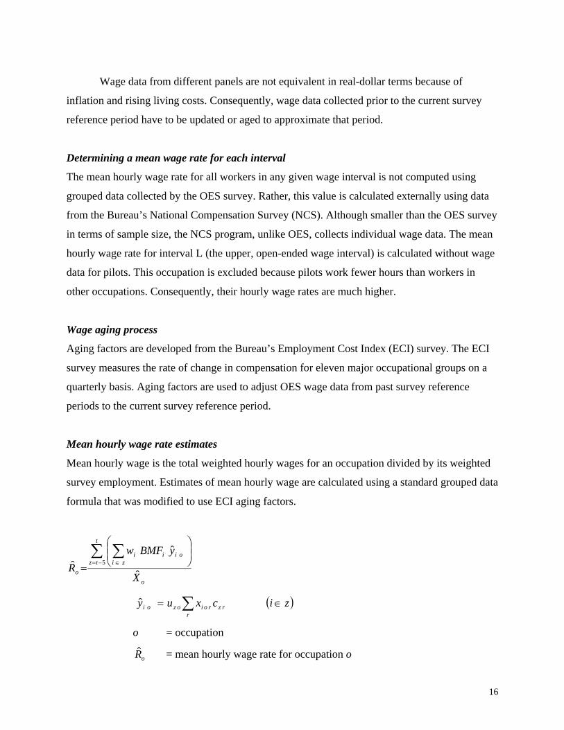
Mean hourly wage rate estimates

Mean hourly wage is the total weighted hourly wages for an occupation divided by its weighted

survey employment. Estimates of mean hourly wage are calculated using a standard grouped data

formula that was modified to use ECI aging factors.

o

t

tz zioiii

o X

yBMFwR ˆ

ˆˆ 5

∑ ∑−= ∈

⎟⎟⎠

⎞⎜⎜⎝

⎛

=

∑=r

rzroiozoi cxuy ( )zi∈

o = occupation

oR = mean hourly wage rate for occupation o

17

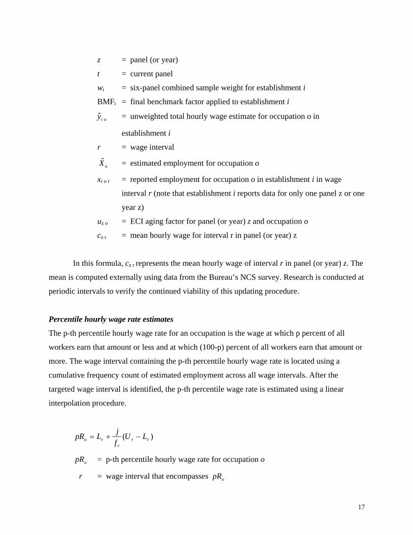
z = panel (or year)

t = current panel

wi = six-panel combined sample weight for establishment i

BMFi = final benchmark factor applied to establishment i

oiy = unweighted total hourly wage estimate for occupation o in

establishment i

r = wage interval

oX = estimated employment for occupation o

xi o r = reported employment for occupation o in establishment i in wage

interval r (note that establishment i reports data for only one panel z or one

year z)

uz o = ECI aging factor for panel (or year) z and occupation o

cz r = mean hourly wage for interval r in panel (or year) z

In this formula, cz r represents the mean hourly wage of interval r in panel (or year) z. The

mean is computed externally using data from the Bureau’s NCS survey. Research is conducted at

periodic intervals to verify the continued viability of this updating procedure.

Percentile hourly wage rate estimates

The p-th percentile hourly wage rate for an occupation is the wage at which p percent of all

workers earn that amount or less and at which (100-p) percent of all workers earn that amount or

more. The wage interval containing the p-th percentile hourly wage rate is located using a

cumulative frequency count of estimated employment across all wage intervals. After the

targeted wage interval is identified, the p-th percentile wage rate is estimated using a linear

interpolation procedure.

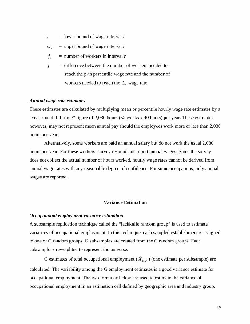
)( rrr

ro LUfjLpR −+=

opR = p-th percentile hourly wage rate for occupation o

r = wage interval that encompasses opR

18

rL = lower bound of wage interval r

rU = upper bound of wage interval r

rf = number of workers in interval r

j = difference between the number of workers needed to

reach the p-th percentile wage rate and the number of

workers needed to reach the rL wage rate

Annual wage rate estimates

These estimates are calculated by multiplying mean or percentile hourly wage rate estimates by a

“year-round, full-time” figure of 2,080 hours (52 weeks x 40 hours) per year. These estimates,

however, may not represent mean annual pay should the employees work more or less than 2,080

hours per year.

Alternatively, some workers are paid an annual salary but do not work the usual 2,080

hours per year. For these workers, survey respondents report annual wages. Since the survey

does not collect the actual number of hours worked, hourly wage rates cannot be derived from

annual wage rates with any reasonable degree of confidence. For some occupations, only annual

wages are reported.

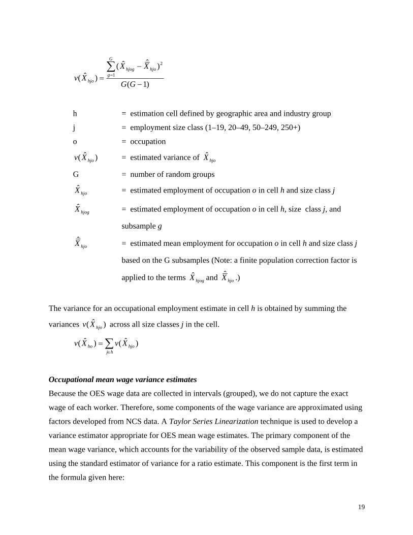
Variance Estimation Occupational employment variance estimation

A subsample replication technique called the “jackknife random group” is used to estimate

variances of occupational employment. In this technique, each sampled establishment is assigned

to one of G random groups. G subsamples are created from the G random groups. Each

subsample is reweighted to represent the universe.

G estimates of total occupational employment ( hjogX ) (one estimate per subsample) are

calculated. The variability among the G employment estimates is a good variance estimate for

occupational employment. The two formulae below are used to estimate the variance of

occupational employment in an estimation cell defined by geographic area and industry group.

19

)1(

)ˆˆ()ˆ( 1

2

−

−=∑=

GG

XXXv

G

ghjohjog

hjo

h = estimation cell defined by geographic area and industry group

j = employment size class (1–19, 20–49, 50–249, 250+)

o = occupation

)ˆ( hjoXv = estimated variance of hjoX

G = number of random groups

hjoX = estimated employment of occupation o in cell h and size class j

hjogX = estimated employment of occupation o in cell h, size class j, and

subsample g

hjoX = estimated mean employment for occupation o in cell h and size class j

based on the G subsamples (Note: a finite population correction factor is

applied to the terms hjogX and hjoX .)

The variance for an occupational employment estimate in cell h is obtained by summing the

variances )ˆ( hjoXv across all size classes j in the cell.

∑∈

=hj

hjoho XvXv )ˆ()ˆ(

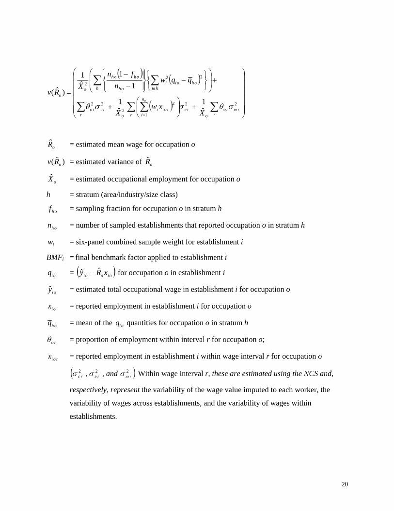
Occupational mean wage variance estimates

Because the OES wage data are collected in intervals (grouped), we do not capture the exact

wage of each worker. Therefore, some components of the wage variance are approximated using

factors developed from NCS data. A Taylor Series Linearization technique is used to develop a

variance estimator appropriate for OES mean wage estimates. The primary component of the

mean wage variance, which accounts for the variability of the observed sample data, is estimated

using the standard estimator of variance for a ratio estimate. This component is the first term in

the formula given here:

20

( ) ( )

( ) ⎟⎟⎟⎟⎟⎟

⎠

⎞

⎜⎜⎜⎜⎜⎜

⎝

⎛

+⎟⎟⎠

⎞⎜⎜⎝

⎛+

+⎟⎟⎠

⎞⎜⎜⎝

⎛

⎭⎬⎫

⎩⎨⎧

−⎪⎭

⎪⎬⎫

⎪⎩

⎪⎨⎧

−

−

=

∑ ∑∑∑

∑ ∑

=

∈

r rrro

ore

n

iroii

orrcro

h hiohoii

oh

ohoh

oo

Xxw

X

qqwn

fnX

Rvo

22

1

22

22

222

ˆ1

ˆ1

11

ˆ1

)ˆ(

ωσθσσθ

oR = estimated mean wage for occupation o

)ˆ( oRv = estimated variance of oR

oX = estimated occupational employment for occupation o

h = stratum (area/industry/size class)

ohf = sampling fraction for occupation o in stratum h

ohn = number of sampled establishments that reported occupation o in stratum h

iw = six-panel combined sample weight for establishment i

BMFi = final benchmark factor applied to establishment i

oiq = ( )oiooi xRy ˆˆ − for occupation o in establishment i

oiy = estimated total occupational wage in establishment i for occupation o

oix = reported employment in establishment i for occupation o

ohq = mean of the oiq quantities for occupation o in stratum h

roθ = proportion of employment within interval r for occupation o;

roix = reported employment in establishment i within wage interval r for occupation o

( )222 ,, rrerc and ωσσσ Within wage interval r, these are estimated using the NCS and,

respectively, represent the variability of the wage value imputed to each worker, the

variability of wages across establishments, and the variability of wages within

establishments.

21

Reliability of the Estimates

Estimates developed from a sample will differ from the results of a census. An estimate based on

a sample survey is subject to two types of error—sampling and nonsampling error. An estimate

based on a census is only subject to nonsampling error.

Nonsampling error

This type of error is attributable to several causes, such as: errors in the sampling frame; an

inability to obtain information for all establishments in the sample; differences in respondents'

interpretation of a survey question; an inability or unwillingness of the respondents to provide

correct information; errors made in recording, coding, or processing the data; and errors made in

imputing values for missing data. Explicit measures of the effects of nonsampling error are not

available.

Sampling errors

When a sample, rather than an entire population, is surveyed, estimates differ from the true

population values that they represent. This difference, or sampling error, occurs by chance, and

its variability is measured by the variance of the estimate or the standard error of the estimate

(the square root of the variance). The relative standard error is the ratio of the standard error to

the estimate itself.

Estimates of the sampling error affecting occupational employment and the mean wage

rate are provided for all employment and mean wage estimates to allow data users to determine

whether those statistics are reliable enough for their needs. Only a probability-based sample can

be used to calculate estimates of sampling error. The formulae used to estimate OES variances

are adaptations of formulae appropriate for the survey design used.

The particular sample used in the OES Survey for a panel is one of a large number of

many possible samples of the same size that could be selected using the same sample design.

Sample estimates from a given design are said to be unbiased when an average of the estimates

from all possible samples yields the true population value. In this case, the sample estimate and

its standard error can be used to construct confidence intervals, or ranges of values with known

probabilities of the true value falling within those ranges. To illustrate, if the process of selecting

a sample from the population is repeated many times, if each sample is surveyed under

22

essentially the same unbiased conditions, and if an estimate and a suitable estimate of its

standard error is made from each sample, then:

1. approximately 68 percent of the intervals from one standard error below to one standard

error above the estimate will include the true population value. This interval is called a

68-percent confidence interval.

2. approximately 90 percent of the intervals from 1.6 standard errors below to 1.6 standard

errors above the estimate will include the true population value. This interval is called a

90-percent confidence interval.

3. approximately 95 percent of the intervals from 2 standard errors below to 2 standard

errors above the estimate will include the true population value. This interval is called a

95-percent confidence interval.

4. almost all (99.7 percent) of the intervals from 3 standard errors below to 3 standard errors

above the estimate will include the true population value.

For example, suppose that an estimated occupational employment total is 5,000, with an

associated estimate of relative standard error of 2.0 percent. On the basis of these data, the

standard error of the estimate is 100 (2 percent of 5,000). To construct a 95-percent confidence

interval, add and subtract 200 (twice the standard error) from the estimate to create a range

spanning from 4,800 to 5,200. Approximately 95 percent of the intervals constructed in this

manner include the true occupational employment if survey methods are nearly unbiased.

Estimated standard errors do not indicate anything other than the magnitude of sampling

error. They are not intended to measure biases in the data or any other kind of nonsampling error.

Particular care should be exercised in the interpretation of small estimates or of small differences

between estimates when the sampling error is relatively large or the magnitude of the bias is

unknown.

Quality control measures

23

The OES survey is a Federal-State cooperative effort that enables States to conduct their

own surveys. A major concern regarding a cooperative program such as OES is the

accommodation of the needs of BLS and other Federal agencies, as well as State-specific

publication needs, despite limited resources while simultaneously standardizing survey

procedures across all 50 States, the District of Columbia, and the U.S. territories. Controlling

sources of nonsampling error in this decentralized environment can be difficult. One important

computerized quality control tool used by the OES survey is the Survey Processing and

Management (SPAM) system. It was developed to provide a consistent and automated

framework for survey processing and to reduce the workload for analysts at the State, regional,

and national levels.

To ensure standardized sampling methods in all areas, the sample is drawn in the national

office. Standardizing data processing activities such as validating the sampling frame, allocating

and selecting the sample, refining mailing addresses, addressing envelopes and mailers, editing

and updating questionnaires, conducting electronic review, producing management reports, and

calculating employment estimates have resulted in the overall standardization of the OES survey

methodology. This has reduced the number of errors in the data files as well as the time needed

to review them.

Other quality control measures used in the OES survey include:

• follow-up mail and telephone solicitations of nonresponding establishments, especially those

that are critical or large

• review of schedules to verify the accuracy and reasonableness of the reported data

• adjustments for atypical reporting units on the data file

• validation of the benchmark employment figures and of the benchmark factors

• validation of the analytical tables of estimates at the NAICS4/5 level

• response analysis studies conducted to assess respondents’ comprehension of the questionnaire

Confidentiality

BLS has a strict confidentiality policy which ensures that the survey sample composition, lists of

reporters, and names of respondents will be kept confidential. Additionally, the policy assures

24

respondents that published figures will not reveal the identity of any specific respondent and will

not allow the data of any specific respondent to be imputed. Each published estimate is screened

to ensure that it meets these confidentiality requirements. To further protect the confidentiality of

the data, the specific screening criteria are not listed in this publication.

Data Presentation

OES estimates are published on the BLS Web site at www.bls.gov/oes/#tables in HTML format.

Included are cross-industry data for the United States as a whole, for individual U.S. States, and

for metropolitan areas, along with U.S. estimates by 3-, 4- and some 5-digit NAICS levels for

industry data. Also provided are downloadable files in EXCEL format. The home page of the

OES program is www.bls.gov/oes. In addition, these tables provide the Relative Standard Error

(RSE) for appropriate estimates of employment and wages.

When updated estimates become available, a BLS news release makes an announcement

providing a summary of U.S. data. The OES program produces an annual publication that

highlights OES data for particular occupations, industries, States, and MSAs.

For additional information, contact the OES staff at (202) 691-6569 or send e-mail to

oesinfo@bls.gov.

Uses

For many years, the OES survey has been a major source of detailed occupational employment

data by industry for the Nation, for States, and for metropolitan areas. This survey provides

information for many data users, including individuals and organizations engaged in planning

vocational education programs, higher education programs, and employment and training

programs. OES data also are used to prepare information for career counseling, for job placement

activities performed at State Workforce Agencies, and for personnel planning and market

research conducted by private enterprises. OES data also is used by the Department of Labor’s

Foreign Labor Certification (FLC) program, which sets the minimum rate at which workers on

work visas in the United States must be paid.

25

Technical References

Executive Office of the President, Office of Management and Budget, Standard Occupational Classification--

Revision for 2010, Federal Register Notice, May 16, 2006

Executive Office of the President, Office of Management and Budget, North American Industry Classification

System, 2002

Executive Office of the President, Office of Management and Budget, Standard Occupational Classification

Manual, 2000

U.S. Department of Labor, Bureau of Labor Statistics, Revising the Standard Occupational Classification System,

Report 929, June 1999.

U.S. Department of Labor, Bureau of Labor Statistics, Occupational Employment and Wages, 1997,

Bulletin 2516, August 1999.

U.S. Department of Labor, Bureau of Labor Statistics, Occupational Employment and Wages, 1998,

Bulletin 2528, June 2000.

U.S. Department of Labor, Bureau of Labor Statistics, Occupational Employment and Wages, 1999,

Bulletin 2545, September 2001.

U.S. Department of Labor, Bureau of Labor Statistics, Occupational Employment and Wages, 2000,

Bulletin 2549, April 2002.

U.S. Department of Labor, Bureau of Labor Statistics, Occupational Employment and Wages, 2001,

Bulletin 2559, June 2003.

U.S. Department of Labor, Bureau of Labor Statistics, Occupational Employment and Wages, May 2003, Bulletin 2567, September 2004

26

U.S. Department of Labor, Bureau of Labor Statistics, Occupational Employment and Wages, May 2004,

Bulletin 2575, September 2005

U.S. Department of Labor, Bureau of Labor Statistics, Occupational Employment and Wages, May 2005,

Bulletin 2585, May 2007.