CFL LIGHT BULB (DIRECT INSTALL) Description of Measure A direct installed screw-based CFL bulb. “Direct installed” bulbs are either supplied to the builder for use in qualifying new homes or installed during the final inspection. Savings do not apply to bulbs that are placed in closets or non-living spaces (attics, unconditioned basements, etc.). Method for Calculating Energy Savings Annual Energy Savings = Δ Watts x Hours x 365/1000 Where: Δ Watts = 2.4 x CFL wattage. This represents an “incandescent to CFL” wattage ratio of 3.4 to 1.

Hours = 2.6 Hours per day (See Note 1)

365 = days per year For example, the annual savings for a 20 watt CFL:

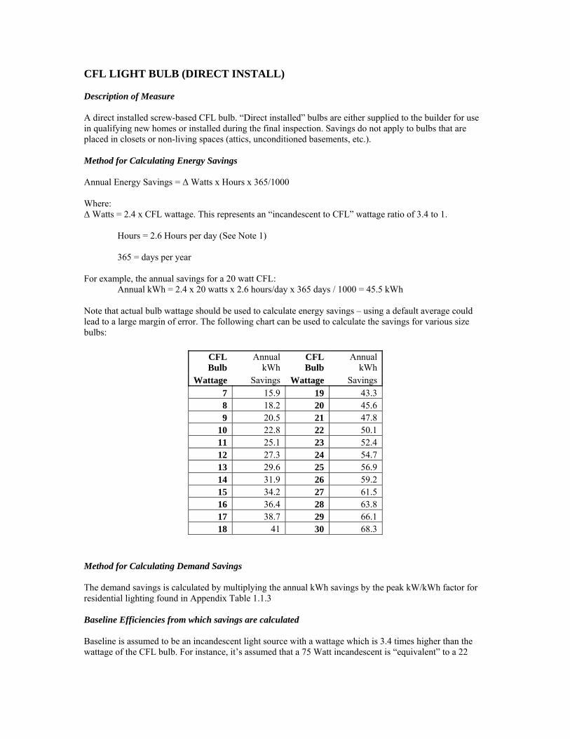
Annual kWh = 2.4 x 20 watts x 2.6 hours/day x 365 days / 1000 = 45.5 kWh Note that actual bulb wattage should be used to calculate energy savings – using a default average could lead to a large margin of error. The following chart can be used to calculate the savings for various size bulbs:

CFL Bulb

Annual kWh

CFL Bulb

Annual kWh

Wattage Savings Wattage Savings7 15.9 19 43.3 8 18.2 20 45.6 9 20.5 21 47.8

10 22.8 22 50.1 11 25.1 23 52.4 12 27.3 24 54.7 13 29.6 25 56.9 14 31.9 26 59.2 15 34.2 27 61.5 16 36.4 28 63.8 17 38.7 29 66.1 18 41 30 68.3

Method for Calculating Demand Savings The demand savings is calculated by multiplying the annual kWh savings by the peak kW/kWh factor for residential lighting found in Appendix Table 1.1.3 Baseline Efficiencies from which savings are calculated Baseline is assumed to be an incandescent light source with a wattage which is 3.4 times higher than the wattage of the CFL bulb. For instance, it’s assumed that a 75 Watt incandescent is “equivalent” to a 22

Watt CFL (22 x 3.4 = 75). For dimmable or three-way CFL bulbs, assume the highest wattage/setting when calculating the baseline equivalent. Compliance Efficiency from which incentives are calculated Energy Star CFL Bulb. Operating Hours 2.6 Hours per day from RLW 2003 Lighting Evaluation (Note 1). Incremental Cost $3.00 Non-Electric Benefits - Annual O&M Cost Adjustments $4.00 per bulb one time benefit. Estimate based on current cost of incandescent bulbs that would be used in place of one CFL. Notes & References Note 1. Northeast Utilities and United Illuminating Retail/Point of Purchase Lighting Program Impact Evaluation, RLW Analytics, April 2003.

CFL FXTURES (NEW HOMES) Description of Measure An Energy Star hardwired fluorescent fixture with pin based bulbs. Fixtures with screw-based (CFL) bulbs are treated as CFL bulbs for savings calculations. Method for Calculating Energy Savings Annual Energy Savings = Δ Watts x Hours x 365/1000 Where:

Δ Watts = 2.4 x fixture wattage (a 3.4 wattage conversion factor). Hours = 3.2 Hours per day (Note 1) 365 = days per year

For example, the annual savings for a 25 watt fixture:

Annual kWh = 2.4 x 25 watts x 3.2 hours/day x 365 days / 1000 = 70.1 kWh Method for Calculating Demand Savings The peak demand savings is calculated by multiplying the annual kWh by the peak demand factor for residential lighting found in Appendix Table 1.1.3 Baseline Efficiencies from which savings are calculated Incandescent fixture with a wattage equal to 3.4 times the wattage of the efficient fluorescent fixture. For dimmable or three-way CFL bulbs, assume the highest wattage/setting when calculating the baseline equivalent. Compliance Efficiency from which incentives are calculated Energy Star hard-wired fixture with equivalent lumen output. Operating Hours 3.2 hours per day from RLW 2003 Lighting Evaluation (Note 1). Incremental Cost $10 Non-Electric Benefits - Annual Fossil Fuel Savings Non-electric benefits have not been identified for this measure. Non-Electric Benefits - Annual O&M Cost Adjustments $14.00 (one-time benefit per fixture). Estimate based on added cost of using incandescent bulbs over the life of the measure. Notes & References Note 1. Northeast Utilities and United Illuminating Retail/Point of Purchase Lighting Program Impact Evaluation, RLW Analytics, April 2003.

SEER 14 MIN AC Description of Measure Central AC system with rated efficiency of 14 SEER or higher. Method for Calculating Energy Savings

A. New Construction: Annual Energy Savings = 500 x size (1/13 – 1/SEER) / 1000 Where:

500 = expected annual full-run hours (Note 1). Size = size of system in Btu 13 = assumed SEER (efficiency) of baseline equipment. SEER = rated SEER (efficiency) of efficient equipment

For example, for a 3 ton (36,000 Btu) 14 SEER system, the annual kWh savings would be = 500 x 36,000 x (1/13 – 1/14) / 1000 = 98.9 kWh. The following chart can be used as a reference to look up the savings for new units:

Size 14

SEER 15

SEER 16

SEER 17

SEER 1 ton 33 61.5 86.5 108.6 2 ton 65.9 123.1 173.1 217.2 3 ton 98.9 184.6 259.6 325.8 4 ton 131.9 246.2 346.2 434.4 5 ton 164.8 307.7 432.7 543

Expected annual kWh cooling savings for various sizes and efficiency of units Note 1: The above chart on energy savings also applies to the Ductless Mini Splits Heat Pump equipments. Note 2: For multi-speed units, a weighted average of the high speed and low speed efficiencies should be used. Assume 70% on low speed and 30% on high speed.

B. Early Retirement: If the contractor identifies an old central air unit still working and the customer agrees to replace it then a savings can be claimed for removing old unit and installing an Energy Star Unit. The following chart can be used as a reference to look up the savings for Early Retirement of old units: Annual Energy Savings = 500 x size (1/Old SEER – 1/New SEER) / 1000 Where:

500 = expected annual full-run hours (Note 1). Size = size of system in Btu Old SEER = Rated SEER (efficiency) of the old unit being replaced. New SEER = Rated SEER (efficiency) of efficient equipment.

Table: Annual Energy savings in kWh per ton

Old Existing Equipment SEER

7.0 7.5 8.0 8.5 9.0 9.5 10.0

13.0 395.60 338.46 288.46 244.34 205.13 170.04 138.46

13.5 412.70 355.56 305.56 261.44 222.22 187.13 155.56

14.0 428.57 371.43 321.43 277.31 238.10 203.01 171.43

14.5 443.35 386.21 336.21 292.09 252.87 217.79 186.21

15.0 457.14 400.00 350.00 305.88 266.67 231.58 200.00

15.5 470.05 412.90 362.90 318.79 279.57 244.48 212.90

New

Equ

ipm

ent S

EE

R

16.0 482.14 425.00 375.00 330.88 291.67 256.58 225.00 For early retirement, the measure life is 18 years. However, the first five years savings are based on the old unit verses an energy star unit (assumes unit would have been installed for another 5 years) and the remaining 13 years savings are based on the new energy star unit verses the baseline. For example, if a 3 ton SEER 8.0 unit was retired and replaced with a new SEER 15 unit, the lifetime savings would be 5x(1050 kWh) + 13x(184.6kWh)=3450 kWh. Note: Retirement savings may only be claimed if retirement is program induced. Method for Calculating Demand Savings Annual kW = size (1/11 – 1/New EER) / 1000 Where:

Size = size of system in Btu/hr EER for a baseline SEER 13 unit = 11 New EER = Rated EER (Energy Efficiency Ratio) of efficient equipment.

Baseline Efficiencies from which savings are calculated A 13 SEER (code minimum) system. Compliance Efficiency from which incentives are calculated 14 SEER or higher (Note 1). Operating Hours 500 hours per year. Incremental Cost $100 per SEER unit per ton above 13. For example, a 3 ton 15 SEER would have an assumed incremental cost of $600.

Non-Electric Benefits - Annual Fossil Fuel Savings Non-electric benefits have not been identified for this measure. Notes & References Note 1. Estimated based on Market Research for the Rhode Island, Massachusetts, and Connecticut Residential HVAC Market, RLW Analytics, December 2002, and supported by ASHRAE hours of use when corrected for oversizing.

HEAT PUMP Description of Measure A heat pump with a heating season performance factor (HSPF) of 8.5 or higher. Note only the heating savings is presented here; cooling savings from an efficient heat pump is the same as the cooling savings for an efficient air conditioner. Utilize methodology in measure 5.2.1 in this manual to determine cooling savings if unit is rated in SEER and 5.3.6 if unit is rated in EER. Method for Calculating Energy Savings

A. New Construction: Annual Energy (heating) Savings = 1,500 x Size (1/7.7 – 1/HSPF) / 1000 Where:

1,500 = estimated annual full-run hours Size = size of system in Btu 7.7 = assumed efficiency of baseline equipment (HSPF Baseline) HSPF = rated Heating Season Performance Factor of efficient equipment

For example, for a 3 ton (36,000 Btu) 9 HSPF system, the annual kWh savings would be = 1,500 x 36,000 x (1/7.7 – 1/9) / 1000 = 1,013 kWh. The following chart can be used as a reference to look up the savings for various sizes and efficiencies:

Size 8.5 9.0 9.5 1 ton 220 338 443 2 ton 440 675 886 3 ton 660 1,013 1,329 4 ton 880 1,351 1,772 5 ton 1,100 1,688 2,215

Expected annual kWh heating savings for various sizes and efficiency of units Note 1: The above chart on energy savings also applies to Ductless Mini Splits Heat Pump equipments. Note 2: For multi-speed units, a weighted average of the high speed and low speed efficiencies should be used. Assume 70% on low speed and 30% on high speed.

B. Early Retirement: The following Table shows the annual energy savings from the installation of old existing equipments with new Energy Star rated heat pumps. Where:

1,500 = Estimated annual full-run hours Size = Size of system in Btu Old HSPF = Heating Season Performance Factor of old existing equipment New HSPF = Heating Season Performance Factor of new Energy Star equipment

If unit heating efficiency is a COP then multiply COP by 3.41 to get HSPF Annual Energy (heating) Savings = 1,500 x Size (1/Old HSPF – 1/New HSPF) / 1000

Table: Annual energy savings in kWh per ton Old Existing Equipment HSPF

5.0 5.2 5.4 5.6 5.8 6.0 6.2 6.4 6.6 6.8 7.0

8.0 1350.0 1211.5 1083.3 964.3 853.4 750.0 653.2 562.5 477.3 397.1 321.4

8.2 1404.9 1266.4 1138.2 1019.2 908.3 804.9 708.1 617.4 532.2 451.9 376.3

8.4 1457.1 1318.7 1190.5 1071.4 960.6 857.1 760.4 669.6 584.4 504.2 428.6

8.6 1507.0 1368.5 1240.3 1121.3 1010.4 907.0 810.2 719.5 634.2 554.0 478.4

8.8 1554.5 1416.1 1287.9 1168.8 1058.0 954.5 857.8 767.0 681.8 601.6 526.0

New

Equ

ipm

ent H

SPF

9.0 1600.0 1461.5 1333.3 1214.3 1103.4 1000.0 903.2 812.5 727.3 647.1 571.4 For early retirement, the measure life is 18 years. However, the first five years savings are based on the old unit verses an energy star unit (assumes unit would have been installed for another 5 years) and the remaining 13 years savings are based on the new energy star unit verses the baseline. For example, if a 3 ton HSPF 6.0 unit was retired and replaced with a new HSPF 9.0 unit, the lifetime savings would be 5x(3000 kWh) + 13x(1013kWh)=3450 kWh. Note: Retirement savings may only be claimed if retirement is program induced.

C. Electric Resistance to Air Source Heat Pump Energy Savings: Table: Annual energy savings in kWh per ton replacing Electric Resistance HP to Energy Star rated Heat Pump.

Old Electric Resistance Unit

COP = 1 (HSPF = 3.4)

8 3028.6

8.2 3083.5

8.4 3135.7

8.6 3185.6

8.8 3233.1

New

Hea

t Pum

p H

SPF

9 3278.6 Method for Calculating Demand Savings The peak demand savings is calculated by multiplying the annual kWh savings by the peak kW/kWh factor for winter heating or summer cooling found in Appendix Table 1.1.3 Baseline Efficiencies from which savings are calculated 7.7 HSPF (code minimum) heat pump. In case of Retrofit the baseline for energy savings calculation is the HSPF rating of the old existing heat pump. Compliance Efficiency from which incentives are calculated 8.5 or higher HSPF heat pump (Note 1) Operating Hours 1500 hours per year

Incremental Cost $400 per ton. Non-Electric Benefits - Annual Fossil Fuel Savings Non-electric benefits have not been identified for this measure.

GEOTHERMAL HEAT PUMP Description of Measure Groumd source heat pump (GSHP) systems. GSHP systems (or “geothermal”), supply heating, cooling, and in some cases water heating (desuperheater or full hot water capability). The savings from those three end-uses are presented separately Method for Calculating Energy Savings The following table was developed from the results of “HVAC Systems in an Energy Star Home: Owning & Operating Costs”, Johnson Research, LLC. The values in the table are given in units per ton of installed cooling capacity.

Heating Consumption

Heating System Consumption Engineering Units Efficiencies

Electric Resistance 5,971 kWh/Ton 100% Air Source Heat Pump 2,504 kWh/Ton 7.7 HSPF Oil Furnace 265 Gallons/Ton 80% AFUE 195 kWh/Ton Gas Furnace 344 Therms/Ton 78% AFUE 240 kWh/Ton GSHP 1,660 kWh/Ton 4 COP Note: Tonnage based on cooling capacity of Geothermal Unit

Cooling Consumption and Summer Demand

System Cooling (kWh/Ton) Efficiency

Summer Demand (kW/Ton)

Electric Resistance 807 13 SEER 1.05 Air Source Heat Pump 807 13 SEER 1.05 Oil Furnace 807 13 SEER 1.05 Gas Furnace 807 13 SEER 1.05 GSHP 541 19.4 EER 0.65 Note: Tonnage based on cooling capacity

Water Heating Consumption System Consumption Units Electric Resistance 4,305 kWh Oil 154 Gallons Gas 215 Therms

Annual kWh savings = annual kWh Heating savings + annual kWh Cooling savings +annual kWh water heating savings The non-commissioning savings calculations below are shown for information only. Savings claimed by this measure will only be the commissioning savings calculated below. It is assumed that customers would have installed geothermal without program intervention.

1) Natural Gas Baseline. a) Heating (kWh) Savings = INCCAP*(240 – (1,660)*(4 /INCOP)) b) Cooling (kWh) Savings = INCCAP*(807 – (541)*(19.4 /INEER)) c) Water Heating (kWh) Savings = 0 – (4,305/INWHCOP) 2) Oil Baseline: a) Heating (kWh) Savings = INCCAP*(195 – (1,660)*(4 /INCOP)) b) Cooling (kWh) Savings = INCCAP*(807 – (541)*(19.4 /INEER)) c) Water Heating (kWh) Savings = 0 – (4,305/INWHCOP) 3) Electric Resistance Baseline: a) Heating (kWh) Savings = INCCAP*(5,971 – (1,660)*(4 /INCOP)) b) Cooling (kWh) Savings = INCCAP*(807 – (541)*(19.4 /INEER)) c) Water Heating (kWh) Savings = 4,304 – (4,305/INWHCOP) 4) Air Source Heat Pump Baseline: a) Heating (kWh) Savings = INCCAP*(2,504 – (1,660)*(4 /INCOP)) b) Cooling (kWh) Savings = INCCAP*(807 – (541)*(19.4 /INEER)) c) Water Heating (kWh) Savings = 4,304 – (4,305/INWHCOP) INCCAP = installed nominal cooling capacity in tons INCOP = GSHP’s rated heating efficiency in COP. System must be tested to verify unit is operating at rated efficiency. INEER = GSHP’s rated Cooling efficiency in EER. System must be tested to verify unit is operating at rated efficiency. INWHCOP = GSHP’s rated water heating efficiency in COP

Use 1 for electric resistance, use 1.2 for desuperheater The baseline is assumed to be GSHP. Therefore the only claimed savings from this measure would be from the commissioning requirement (and perhaps shell savings). Commissioning savings are assumed to be 10% of the theoretical usage: Heating kWh savings = (166 kWh/ton)(ICCAP)(4)/(INCOP) Cooling kWh savings = (54.1 kWh/ton)(ICCAP)(19.4)/(INEER)

Method for Calculating Demand Savings The savings calculations below are shown for information only. Savings claimed by this measure will only be the commissioning savings calculated above. It is assumed that customers would have installed geothermal without program intervention. For retrofit Projects: Summer Demand savings = Cooling (kW) savings + Water heating (kW) savings

a) Cooling (kW) savings = CF*INCCAP*(1.05 – 0.62*19.4/INEER)

b) Water Heating (kW) savings = (Water heating (kWh) savings) / 8,760 For New construction projects:

a) Cooling (kW) demand savings = CF*INCCAP*0.062*19.4/INEER CF = Residential central cooling coincidence factor Baseline Efficiencies from which savings are calculated It is assumed that the home would have a ground source heat pump without program intervention. However, it is assumed that the system would not be commissioned. Therefore, the baseline is an uncommissioned ground source heat pump, and savings is based on the commissioning (10%) savings (in addition to any shell savings through the Residential New Construction Program). System Replacement: The existing system will determine the heating and water heating baseline. Central air with a 13 SEER is the assuming cooling baseline. Incremental Cost Typically, incremental cost will range from $8,000 to $20,000 based on system size and system baseline. A rough estimate of incremental cost would be about $3,000 per ton. Non-Electric Benefits - Annual Fossil Fuel Savings Fossil Fuel savings = fossil fuel heating savings + Fossil fuel water heating savings Natural Gas Baseline:

Fossil fuel savings (therms) = INCCAP*344 + 215 Oil Baseline:

Fossil Fuel savings (gallons) = INCCAP*298 + 154

AC SYS TUNE-UP Description of Measure This measure applies to diagnostic tune-up using the Service Assistant and is based on the measured changes in the efficiency index (EI) as measured with the Service Assistant Tool. This savings estimate was developed by UI and CL&P in April, 2006. Method for Calculating Energy Savings Annual Energy Savings (kWh) = 12 x Capacity x EFLH x (1/EIb – 1/EIa)

SEER Capacity - Air conditioning units rated capacity in tons 12 - Conversion from tons to kBTU’s SEER - Seasonal energy efficiency ratio (nameplate) EIb – Efficiency index before (output from tool) EIa – Efficiency index after (output from tool) EFLH – Equivalent Full Load Hours (assumed to be 500) IMPORTANT – The following recommendations must be followed in order for savings from a tuneup to be valid.

1) On the occasion that only one reading is taken or EIa < EIb, the savings defaults to 0 and “deemed” savings is not claimed.

2) Minimum outdoor temperature must be 55 Degrees F and 65 Degrees F for a TXV System. “Tents” should not be used to increase the ambient temperature around the condensing unit.

3) System must be running for 10 – 15 minutes prior to taking the first (initial) reading. 4) Compressor must be fully loaded (high speed for multi-speed units) and running at steady state

efficiency. 5) A reasonable indoor load must be maintained throughout the test or the results. Therefore, return

air must be at least 65 degrees F wet bulb and/or 80 degrees F dry bulb temperature. 6) Units that have been tuned-up within measure life time period specified in Table 1.4 can not claim

additional (double-counted) savings since the savings has already been. Method for Calculating Demand Savings Demand Savings (kW) = 12 x Capacity x DF x (1/EIb – 1/EIa)

SEER x 0.875 DF – diversity factor 0.875 – Conversion from SEER to EER. Baseline Efficiencies from which savings are calculated The baseline efficiency is the nameplate SEER multiplied by the EIb. Compliance Efficiency from which incentives are calculated An HVAC system that has documented performance testing using the Service Assistant. Operating Hours The full load operating hours for CT are assumed to be 500 hours / year.

Total Cost The cost to the contractor for each tune-up is assumed to be $125, but costs may vary based on the contractor and geographic location. Also, $125 is assumed to be the minimum cost and is expected to only cover the diagnostic portion of the test in most situations. If significant problems are uncovered during the diagnostic portion of the test, the cost is expected to rise. Non-Electric Benefits - Annual Fossil Fuel Savings Non-electric benefits have not been identified for this measure.

DUCT SEALING Description of Measure Ducts sealed to reduce outside infiltration. Duct improvements (sealing) should be verified with duct blaster test at 25 Pa using an approved test method. Alternative test methods (subtraction method, flow hood method, delta Q, etc) will generally yield inconsistent results and are not permitted. Note that REM savings (5.4.1) and BOP savings (5.4.2) includes duct sealing savings. Therefore, this measure does NOT apply to homes that are already claiming savings as one of these measures. This is a stand-alone measure and is not intended to be applied to homes that fall into one of these tracks. Method for Calculating Energy Savings

A) New Construction: The results below are engineering estimates of expected savings from verified duct sealing for new construction. This savings does NOT apply to Energy Star Homes. For those homes, savings should be calculated using the UDRH (see 5.4.1 REM Savings).

Savings per 1000 Square Feet Conditioned Space

Duct Blaster Results (outside leakage per 100 sq ft conditioned space at 25 Pa)

Heating (MBtu)

Geothermal kWh Savings

Heating (kWh Fan

Savings) kWh

(Cooling) 8 3.1 227 25 101 7 3.9 286 31 127 6 4.7 344 38 152 5 5.5 403 44 177 4 6.3 461 50 203 3 7.0 513 56 228 2 7.8 571 62 253 1 8.6 630 69 279 0 9.4 689 75 304

B) Retrofit

Savings for existing ducts that are sealed. Savings must be verified by measuring outside duct leakage at 25 Pascals using standard duct blaster testing procedures.

Duct Blaster Savings at 25 Pa

Heating (MBtu)

Heating (Resistance)

Heating (Heat

Pumps) Heating

(Geothermal)

kWh Fan Heating Savings

kWh (Cooling)

Average Basement Leakage 5.2 1523 762 507 44 159Average Attic Leakage 8.1 2373 1187 791 65 234Average (basement and attic) 6.7 1948 974 649 55 197Savings for 100 CFM at 25 Pa duct leakage reduction

Method for Calculating Demand Savings The demand savings is calculated using peak factors found in Table 1.1.3 in the Appendix.

Baseline Efficiencies from which savings are calculated Ducts that have not been sealed. Compliance Efficiency from which incentives are calculated Duct sealed to reduce outside leakage. Incremental Cost Actual cost or $100 per 1000 square feet. Non-Electric Benefits - Annual Fossil Fuel Savings

A) New Construction: The heating savings (above) can be converted to appropriate fossil fuel units of measure Savings per 1000 Square feet Conditioned Space

Savings per 1000 Square Feet Conditioned Space

Duct Blaster Results (outside leakage per 100 sq ft conditioned space at 25 Pa)

Heating (MBtu) Gallons Oil Therms Gas

Gallons Propane

8 3.1 29.5 41.7 46.3 7 3.9 37.1 52.2 57.9 6 4.7 44.8 62.5 69.4 5 5.5 52.4 73.0 81.1 4 6.3 60.0 83.3 92.7 3 7.0 66.7 93.9 104.3 2 7.8 74.3 104.3 115.8 1 8.6 81.9 114.7 127.5 0 9.4 89.5 125.1 139.0

Estimated savings values are take into account average expected system efficiency of 75%. In addition, there may be some non-electric benefits due to better comfort and small system size. However, due to their indeterminate nature, it is difficult to rigorously quantify their value with reasonable certainty.

B) Retrofit

Duct Blaster Savings at 25 Pa

Heating (MBtu)

Gallons Oil

Therms Gas

Gallons Propane

Average Basement Leakage 5.2 50.0 70.0 77.8 Average Attic Leakage 8.1 76.9 107.6 119.6 Average (basement and attic) 6.7 63.5 88.9 98.7 Savings for 100 CFM at 25 Pa duct leakage reduction

Estimated savings values are take into account average expected system efficiency of 75%.

HEAT PUMP - DUCTLESS Description of Measure Ductless heat pumps. Method for Calculating Energy Savings Heating Savings is calculated using the lesser of the heating capacity of the unit(s) OR the load of the house, the region IV HSPF, and 1500 full load hours. Estimated heating savings should be compared with bill data for reasonableness. Annual Energy (heating) Savings = 1,500 x Size (1/HSPF(baseline) – 1/HSPF(new)) / 1000 Where:

1,500 = estimated annual full-run hours Size = size of system in Btu HSPF = Heating Season Performance Factor

Cooling savings is calculated using the rated SEER and 500 full load hours. Annual Energy (cooling) Savings = 500 x size (1/SEER(baseline) – 1/SEER(new)) / 1000 Where:

500 = expected annual full-run hours. Size = size of system in Btu SEER = Seasonal Energy Efficiency Ratio

Method for Calculating Demand Savings Demand Savings is calculated using the peak factors in Appendix Table 1.1.3 Baseline Efficiencies from which savings are calculated For retrofit, baseline efficiency is the actual existing efficiency for both heating and cooling. In situations where the actual baseline efficiency us unknown, use the following table:

Technology Baseline Retrofit Efficiency

Baseline New Construction

Electric Resistance Heating 3.41 HSPF N/A Heat Pump (heating) 5.0 HSPF 7.7 HSPF Window AC 7.5 EER/SEER 13 SEER Central AC (or heat pump) Cooling 10 SEER 13 SEER NO AC Present 0 (negative cooling savings) 13 SEER

Operating Hours 1500 hours heating 500 hours cooling Incremental Cost For retrofit, the incremental cost is assumed to be $4,000 + $2,000*(# of zones-1).

i.e. one zone costs $4,000, two zones cost $6,000 etc. A “zone” is a separate air handler regardless of the number of condensing units. For new construction, the incremental cost is $500 Non-Electric Benefits - Annual Fossil Fuel Savings Non-electric benefits have not been identified for this measure.

CFL BULBS (RETAIL) Description of Measure A screw-based (integrated ballast) compact fluorescent light bulb. Typical CFL wattage is between 9 and 23 watts. Method for Calculating Energy Savings Gross Annual Energy Savings = Δ Watts x Hours x 365/1000 Where:

Δ Watts = 2.4 x CFL wattage based on a 3.4 wattage ratio (Note 1). Hours = 2.6 Hours per day (Note 2). 365 = days per year

For example, the annual savings for a 20 watt CFL:

Annual kWh = 2.4 x 20 watts x 2.6 hours/day x 365 days / 1000 = 45.6 kWh Note that actual bulb wattage should be used to calculate energy savings. See the chart below for gross and net savings for bulbs of various wattages. The overall realization rate is 76% and includes the effects of spillover, free-ridership and installation rates (Note 2) The following chart can be used to look up gross (without impact factors) and net (with impact factors) savings for various size bulbs. The gross savings numbers were generated using the savings algorithm above and the net savings numbers were generated by applying the realization rate above to the gross savings:

CFL Bulb Wattage

Gross Annual

kWh Savings

Net Annual kWh

SavingsCFL Bulb

Wattage

Gross Annual

kWh Savings

Net Annual kWh

Savings 7 15.9 12.1 19 43.3 32.9 8 18.2 13.8 20 45.6 34.6 9 20.5 15.6 21 47.8 36.4

10 22.8 17.3 22 50.1 38.1 11 25.1 19.0 23 52.4 39.8 12 27.3 20.8 24 54.7 41.5 13 29.6 22.5 25 56.9 43.3 14 31.9 24.2 26 59.2 45.0 15 34.2 26.0 27 61.5 46.7 16 36.4 27.7 28 63.8 48.5 17 38.7 29.4 29 66.1 50.2 18 41.0 31.2 30 68.3 51.9

Gross and Net Annual Savings for bulbs. Note that the net savings in this chart assumes that sales data is available for the bulb.

Method for Calculating Demand Savings The demand savings is calculated by multiplying the annual kWh savings by the appropriate peak factors found in Appendix Table 1.1.3 Baseline Efficiencies from which savings are calculated Baseline is assumed to be an incandescent light source with a wattage which is 3.4 times higher than the wattage of the CFL bulb. For instance, it’s assumed that a 75 Watt incandescent is “equivalent” to a 22 Watt CFL (22 x 3.4 = 75). For dimmable or three-way CFL bulbs, assume the highest wattage/setting when calculating the baseline equivalent. Compliance Efficiency from which incentives are calculated Energy Star screw-based bulb with equivalent lumen output. Operating Hours 2.6 Hours per day estimate (Note 1). Incremental Cost $2.00 assumed average. Range is between $1 and $10, however most bulbs currently in the lighting program are towards the lower end of this price spectrum. Non-Electric Benefits - Annual O&M Cost Adjustments $4.00 per bulb one time benefit. Estimate based on current cost of incandescent bulbs that would be used in place of one CFL. Notes & References Note 1. Hours of use is an estimate based on various recent evaluation work including: CFL Metering Study, (California), KEMA Inc. 2005. Note 2. Northeast Utilities and United Illuminating Retail/Point of Purchase Lighting Program Impact Evaluation, RLW Analytics, April 2003. Note 3. In cases where sales data is not available, a 35% installation rate should be used (half of the current installation rate of 70%) based on an assumption that half of the bulbs with no sales data make it into the marketplace and produce savings.

PORTABLE LAMPS Description of Measure An Energy Star portable (plug type) light fixture with pin-based bulbs (i.e. table lamp, desk lamp, etc.). Note that torchieres are not included here; rather they are handled as a separate measure. Method for Calculating Energy Savings Annual Energy Savings = Δ Watts x Hours x 365/1000 Where:

Δ Watts = 2.4 x fixture wattage (3.4 wattage conversion factor). Hours = 3.2 Hours per day (Note 1) 365 = days per year

For example, the annual savings for a 25 watt fixture:

Annual kWh = 2.4 x 25 watts x 3.2 hours/day x 365 days / 1000 = 70.1 kWh Method for Calculating Demand Savings The peak demand savings is calculated by multiplying the annual kWh savings by the peak kW/kWh factor for residential lighting found in Appendix Table 1.1.3 Baseline Efficiencies from which savings are calculated Incandescent portable fixture with a wattage equal to 3.4 times the wattage of the efficient fluorescent fixture. For dimmable or three-way products, assume the highest wattage/setting when calculating the baseline equivalent. Compliance Efficiency from which incentives are calculated Energy Star lamp with equivalent lumen output. Operating Hours 3.2 hours per day from RLW 2003 Lighting Evaluation. Note 1. Incremental Cost $10 Non-Electric Benefits - Annual O&M Cost Adjustments $6.00 one-time benefit per fixture. Notes & References Note 1. Northeast Utilities and United Illuminating Retail/Point of Purchase Lighting Program Impact Evaluation, RLW Analytics, April 2003.

TORCHIERE Description of Measure Energy Star torchiere (fixture). Method for Calculating Energy Savings Annual Energy Savings = Δ Watts x Hours x 365/1000 (Note 1) Where:

Δ Watts = the lesser of 2.4 x fixture wattage (3.4 wattage conversion factor). or 190 – fixture Wattage (Note 2). Hours = 3.2 Hours per day 365 = days per year

For example, the annual savings for a 55 watt torchiere fixture:

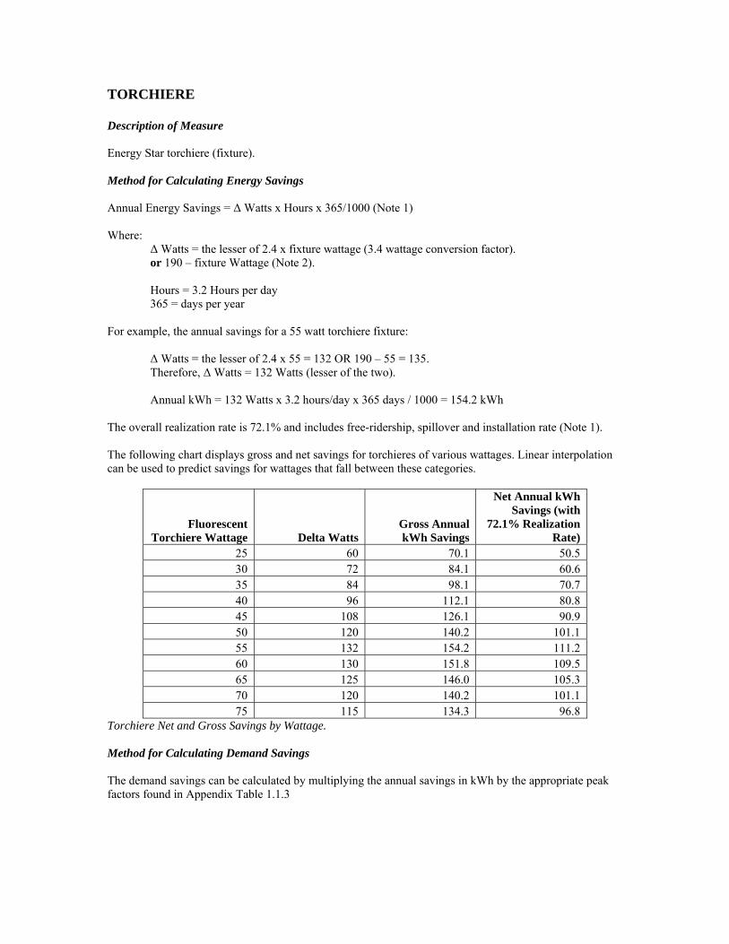
Δ Watts = the lesser of 2.4 x 55 = 132 OR 190 – 55 = 135. Therefore, Δ Watts = 132 Watts (lesser of the two).

Annual kWh = 132 Watts x 3.2 hours/day x 365 days / 1000 = 154.2 kWh

The overall realization rate is 72.1% and includes free-ridership, spillover and installation rate (Note 1). The following chart displays gross and net savings for torchieres of various wattages. Linear interpolation can be used to predict savings for wattages that fall between these categories.

Fluorescent Torchiere Wattage Delta Watts

Gross Annual kWh Savings

Net Annual kWh Savings (with

72.1% Realization Rate)

25 60 70.1 50.5 30 72 84.1 60.6 35 84 98.1 70.7 40 96 112.1 80.8 45 108 126.1 90.9 50 120 140.2 101.1 55 132 154.2 111.2 60 130 151.8 109.5 65 125 146.0 105.3 70 120 140.2 101.1 75 115 134.3 96.8

Torchiere Net and Gross Savings by Wattage. Method for Calculating Demand Savings The demand savings can be calculated by multiplying the annual savings in kWh by the appropriate peak factors found in Appendix Table 1.1.3

Baseline Efficiencies from which savings are calculated Incandescent or halogen torchiere with a wattage equal to 3.4 times the wattage of the efficient fluorescent fixture. For dimmable or three-way products, assume the highest wattage/setting when calculating the baseline equivalent. Compliance Efficiency from which incentives are calculated Energy Star torchiere with equivalent lumen output. Operating Hours 3.2 hours per day. Incremental Cost $10 Non-Electric Benefits - Annual O&M Cost Adjustments $5.00 (one-time benefit per fixture). Estimate based on increased cost of incandescent bulbs that would be used in the baseline case. Notes & References Note 1. Savings assumptions including impact factors are from the following: Northeast Utilities and United Illuminating Retail/Point of Purchase Lighting Program Impact Evaluation, RLW Analytics, April 2003. Note 2. Public Act 04-85, An Act Concerning Energy Efficiency Standards, July 2004, limits torchiere wattage to 190 Watts. Therefore, the baseline is capped at 190 watts and the Δ Wattage is limited by this cap.

FIXTURE (HARD WIRED) Description of Measure An Energy Star hardwired fluorescent fixture with pin based bulbs. Note that fixtures with screw-based (CFL) bulbs are treated as CFL bulbs for savings calculations. Method for Calculating Energy Savings Annual Energy Savings = Δ Watts x Hours x 365/1000 (Note 1). Where:

Δ Watts = 2.4 x fixture wattage (a 3.4 wattage conversion factor). Hours = 3.2 Hours per day 365 = days per year

For example, the annual savings for a 25 watt fixture:

Annual kWh = 2.4 x 25 watts x 3.2 hours/day x 365 days / 1000 = 70.1 kWh For fixtures with multiple bulbs, the wattage is the total wattage of all bulbs (not the wattage of one bulb). Method for Calculating Demand Savings The demand savings can be calculated by multiplying the annual savings in kWh by the appropriate peak factors found in Appendix Table 1.1.3 Baseline Efficiencies from which savings are calculated Incandescent fixture with a wattage equal to 3.4 times the wattage of the efficient fluorescent fixture. For dimmable or three-way CFL bulbs, assume the highest wattage/setting when calculating the baseline equivalent. Compliance Efficiency from which incentives are calculated Energy Star hard-wired fixture with equivalent lumen output. Operating Hours 3.2 hours per day from RLW 2003 Lighting Evaluation (Note 1). Incremental Cost $10 Non-Electric Benefits - Annual O&M Cost Adjustments $14.00 (one-time benefit per fixture). Estimate based added cost of using incandescent bulbs over the life of the measure. Notes & References Note 1. Savings assumptions including impact factors are from the following: Northeast Utilities and United Illuminating Retail/Point of Purchase Lighting Program Impact Evaluation, RLW Analytics, April 2003.

CEILING FAN & LIGHTS Description of Measure Energy Star ceiling fan/light combination. Method for Calculating Energy Savings Note that only the energy savings from the light is considered. Therefore, savings for this measure is based on the light wattage and is identical to the savings for a light fixture. Fan motor savings is negligible, and cooling savings has not been determined. Annual Energy Savings = Δ Watts x Hours x 365/1000 (Note 1). Where:

Δ Watts = 2.4 x fixture wattage (a 3.4 wattage conversion factor). Hours = 3.2 Hours per day 365 = days per year

For example, the annual savings for a qualifying fan/light with a 25 watt light source:

Annual kWh = 2.4 x 25 watts x 3.2 hours/day x 365 days / 1000 = 70.1 kWh For fans with multiple bulbs, the wattage is the total wattage of all bulbs. For instance, if a ceiling fan has four 20 watt bulbs, the savings would be based on an 80 Watt light source. Method for Calculating Demand Savings The demand savings can be calculated by multiplying the annual savings in kWh by the appropriate peak factors found in Appendix Table 1.1.3 Baseline Efficiencies from which savings are calculated Fan/light combination with an incandescent light source wattage equal to 3.4 times the light source wattage of the Energy Star fan/light combination. Compliance Efficiency from which incentives are calculated Energy Star fan/light combination with fluorescent light source. Operating Hours 3.2 hours per day from RLW 2003 Lighting Evaluation (Note 1). Incremental Cost $10 Non-Electric Benefits - Annual O&M Cost Adjustments $14.00 (one-time benefit per fixture). Estimate based added cost of using incandescent bulbs over the life of the measure. Notes & References Note 1. Savings assumptions including impact factors are from the following: Northeast Utilities and United Illuminating Retail/Point of Purchase Lighting Program Impact Evaluation, RLW Analytics, April 2003.

ROOM WINDOW AIR CONDITIONER Description of Measure Room air conditioners meeting the minimum qualifying efficiencies established by the Energy Star Program that are purchased from vendors participating in negotiated cooperative promotions. Method for Calculating Energy Savings The savings is the difference in consumption between the new Energy Star unit and the base unit (minimum federal efficiency standard). Annual kWh Savings = 500 hours * BTU/h Rating * (1/Fed Std EER - 1/Actual EER)/1000W/ kW

EER Rating > 9.7 10 10.7 11 11.5 12 Fed Std E-Star min BTU/h Rating

5,000 0.0 7.7 24.1 30.5 40.3 49.4 6,000 0.0 9.3 28.9 36.6 48.4 59.3

EER Rating > 9.8 10 10.8 11 11.5 12 Fed Std E-Star min

8,000 0.0 8.2 37.8 44.5 60.3 74.8 10,000 0.0 10.2 47.2 55.7 75.4 93.5 11,000 0.0 11.2 52.0 61.2 83.0 102.9 12,000 0.0 12.2 56.7 66.8 90.5 112.2 13,000 0.0 13.3 61.4 72.4 98.0 121.6

EER Rating > 9.7 10 10.7 11 11.5 12 Fed Std E-Star min

14,000 0.0 21.6 67.4 85.3 113.0 138.3 15,000 0.0 23.2 72.3 91.4 121.0 148.2 16,000 0.0 24.7 77.1 97.5 129.1 158.1 17,000 0.0 26.3 81.9 103.6 137.2 168.0 18,000 0.0 27.8 86.7 109.7 145.2 177.8

Method for Calculating Demand Savings The demand saving is calculated by multiplying the annual savings by the summer peak demand factor for residential cooling found in Table 1.1.3 in the Appendix. Baseline Efficiencies from which savings are calculated The baseline efficiencies are the Federal Standards shown in the table above. Compliance Efficiency from which incentives are calculated The compliance efficiencies are the Energy Star Efficiencies shown in the table above. Operating Hours The full load operating hours for CT are assumed to be 500 hours per year.

Incremental Cost The incremental cost of a new Energy Star unit is assumed to be $50. Non-Electric Benefits - Annual Fossil Fuel Savings Non-electric benefits have not been identified for this measure. Non-Electric Benefits - Annual Water Savings Non-electric benefits have not been identified for this measure. Non-Electric Benefits - Annual O&M Cost Adjustments Non-electric benefits have not been identified for this measure.

CLOTHES WASHER Description of Measure Residential clothes washers meeting the minimum qualifying efficiency standards establishes under the Energy Star Program. Method for Calculating Energy Savings The savings shown below for program planning purposes is the average for washers based on an expected fuel mix. Table1: Annual Energy Savings

MEF 20% 80% 24% 48% 8%

Clothes Washers Incremental Cost

Electric Water Heater Savings

Fossil Fuel Water Heater Savings

Annual Water Savings Mix

Electric (kWh)

Fossil Fuel (BTU)

Electric (kWh)

Fossil Fuel (BTU) (gallons)

Electric (kWh)

Fossil Fuel (BTU)

Natural Gas (CCF) Oil (Gal) Other (BTU)

Savings - New Units

Baseline 1.26 0 0 0 0 0 0 0 0 0 0 0

Energy Star 1.72 290 254 0 15.0 900,000 6,993 62.8 720,000 2.16 3.09 72,000

Tier 3 2.20 609 0 22.4 1,680,531 7,397 139.7 1,344,425 4.03 5.76 134,442

Early Retirement

Typical Washer - 0 0 0 0 0 0 0 0 0 0 0

Energy Star 1.72 565 0 50.0 3,900,000 9,932 153.0 3,120,000 9.36 13.37 312,000

Tier 3 2.20 920 0 57.4 4,680,531 10,336 229.9 3,744,425 11.23 16.05 374,442

For new units, the weighted average savings for tier 3 washers and all fuel types is 139.7 kWh compared to the federal minimum baseline. For early retirement, the measure life is 14 years. However, the first four years savings (229.9 kWh weighted all fuels) are based on the old washer (typical) verses a tier 3 washer (assumes old washer would have been used another 4 years) and the remaining 10 years savings (139.7 kWh weighted all fuels) are based on the new Tier 3 washer verses the baseline. This assumes that the customer replaces the existing unit with a Tier 3 model. Note: Retirement savings may only be claimed if retirement is program induced. Method for Calculating Demand Savings The peak demand savings is calculated by multiplying the annual kWh savings by the peak kW/kWh factor for winter or summer domestic water heating found in Appendix Table 1.1.3. Baseline Efficiencies from which savings are calculated The baseline efficiency is the efficiency of a washer meeting the federal minimum std. Compliance Efficiency from which incentives are calculated The compliance efficiency to receive an incentive is that of an Energy Star Washer.

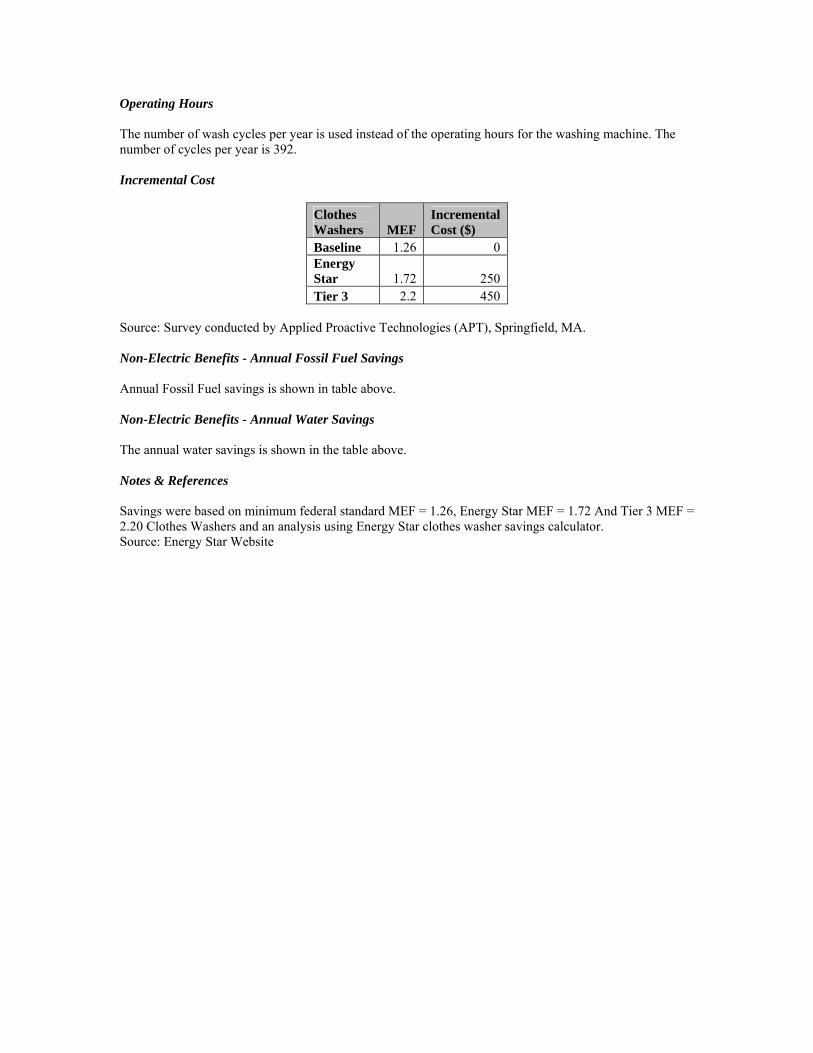
Operating Hours The number of wash cycles per year is used instead of the operating hours for the washing machine. The number of cycles per year is 392. Incremental Cost

Clothes Washers MEF

Incremental Cost ($)

Baseline 1.26 0 Energy Star 1.72 250 Tier 3 2.2 450

Source: Survey conducted by Applied Proactive Technologies (APT), Springfield, MA. Non-Electric Benefits - Annual Fossil Fuel Savings Annual Fossil Fuel savings is shown in table above. Non-Electric Benefits - Annual Water Savings The annual water savings is shown in the table above. Notes & References Savings were based on minimum federal standard MEF = 1.26, Energy Star MEF = 1.72 And Tier 3 MEF = 2.20 Clothes Washers and an analysis using Energy Star clothes washer savings calculator. Source: Energy Star Website

DISHWASHER Description of Measure Energy Star Dishwasher Method for Calculating Energy Savings Table1: Annual Energy

EF 20% 80% 24% 48% 8%

Dishwashers Incremental Cost

Electric Water Heater Savings

Fossil Fuel Water Heater Savings

Annual Water Savings Mix

Electric (kWh)

Fossil Fuel (BTU)

Electric (kWh)

Fossil Fuel (BTU) (gallons)

Electric (kWh)

Fossil Fuel (BTU)

Natural Gas (CCF) Oil (Gal) Other (BTU)

Savings - New Units

Baseline 6 0 0 0 0 0 0 0 0 0 0 0

Energy Star 7 50 51.0 0 23.0 250,000 430 28.6 200,000 0.60 1.20 20,000

Early Retirement

Typical Dishwasher - 0 0 0 0 0 0 0 0 0 0 0

Energy Star 0.7 500 125.9 0 55.4 287,000 559 69.5 229,600 0.6888 0.98 22,960

For early retirement, the measure life is 12 years. However, the first three years savings (69.5 weighted all fuels) are based on the old dishwasher (typical) verses the new Energy star dishwasher (assumes old dishwasher would have been used another 3 years) and the remaining 9 years savings (28.6 weighted all fuels) are based on the new energy star dishwasher verses the baseline. Note: Retirement savings may only be claimed if retirement is program induced. Method for Calculating Demand Savings The demand savings for the summer or winter peak period is calculated by multiplying the annual kWh savings by a summer or winter peak coincidence factor for domestic water heating found in Appendix Table 1.1.3. Baseline Efficiencies from which savings are calculated The baseline efficiencies are the Federal Standard values shown in the table above. Operating Hours Operating hours do not apply since the Federal Standards are written in units of cycles/kWh. Incremental Cost The Energy Star web site uses $50 as the incremental cost between an Energy Star model and a Federal Standard model. Source: Survey conducted by APT Non-Electric Benefits - Annual Fossil Fuel Savings Annual Fossil Fuel savings is shown in table above.

Non-Electric Benefits - Annual Water Savings The annual water savings is shown in the table above. Source: Energy Star Website Notes & References www.energystar.gov

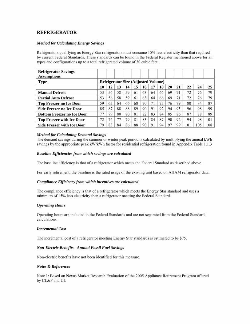
REFRIGERATOR Method for Calculating Energy Savings Refrigerators qualifying as Energy Star refrigerators must consume 15% less electricity than that required by current Federal Standards. These standards can be found in the Federal Register mentioned above for all types and configurations up to a total refrigerated volume of 30 cubic feet. Refrigerator Savings Assumptions Type Refrigerator Size (Adjusted Volume) 10 12 13 14 15 16 17 18 20 21 22 24 25 Manual Defrost 53 56 58 59 61 63 64 66 69 71 72 76 79 Partial Auto Defrost 53 56 58 59 61 63 64 66 69 71 72 76 79 Top Freezer no Ice Door 59 63 64 66 68 70 71 73 76 79 80 84 87 Side Freezer no Ice Door 85 87 88 88 89 90 91 92 94 95 96 98 99 Bottom Freezer no Ice Door 77 79 80 80 81 82 83 84 85 86 87 88 89 Top Freezer with Ice Door 72 76 77 79 81 83 84 87 90 92 94 98 101 Side Freezer with Ice Door 79 83 84 86 88 90 91 94 97 99 101 105 108

Method for Calculating Demand Savings The demand savings during the summer or winter peak period is calculated by multiplying the annual kWh savings by the appropriate peak kW/kWh factor for residential refrigeration found in Appendix Table 1.1.3 Baseline Efficiencies from which savings are calculated The baseline efficiency is that of a refrigerator which meets the Federal Standard as described above. For early retirement, the baseline is the rated usage of the existing unit based on AHAM refrigerator data. Compliance Efficiency from which incentives are calculated The compliance efficiency is that of a refrigerator which meets the Energy Star standard and uses a minimum of 15% less electricity than a refrigerator meeting the Federal Standard. Operating Hours Operating hours are included in the Federal Standards and are not separated from the Federal Standard calculations. Incremental Cost The incremental cost of a refrigerator meeting Energy Star standards is estimated to be $75. Non-Electric Benefits - Annual Fossil Fuel Savings Non-electric benefits have not been identified for this measure. Notes & References Note 1: Based on Nexus Market Research Evaluation of the 2005 Appliance Retirement Program offered by CL&P and UI.

ROOM AC RETIREMENT Description of Measure This measure applies to old room air conditioners which are in working condition, but are turned in to a demanufacturing facility where they are properly disassembled, with all materials recycled where possible. Method for Calculating Energy Savings For early retirement, the measure life is 12 years. However, the first 3 years savings are based on the old air conditioner (assumes old unit would have been used another 3 years) and the remaining 9 years savings are based on the new energy star air conditioner. The savings are estimated to be 191kWh per year for the first three years and 58 kWh for the remaining 9 years. A realization factor of 20.7% should be applied for the first 3 years and 26.0% for the remaining 9 years. Note: Retirement savings may only be claimed if retirement is program induced. Energy Savings and Realization rate base on Impact, Process, and Market study of CT Appliance retirement Program, Nexus Market Research, Inc., December 2005, Table 2.13, page 25 Method for Calculating Demand Savings Demand savings in kW is calculated by multiplying the annual savings in kWh by the summer system peak kW/kWh factor found in Appendix Table1.1.3. Baseline Efficiencies from which savings are calculated The Federal Standard baseline efficiency is 9.7BTU/W. Compliance Efficiency from which incentives are calculated The unit retired must be in working condition when retired. Operating Hours The full load operating hours for CT is assumed to be 500 hours per year. Total Cost The cost to pick up and demanufacture an AC unit is $65.00 plus any customer incentive.

REFRIGERATOR RETIREMENT Description of Measure This measure is for the retirement and demanufacturing of refrigerators. Refrigerators are picked up at the customer’s premises, and removed to a central facility operated by a contractor where they are disassembled, with all material recycled where practical. The refrigerators are required to be in working order, preferably having been in operation as a second or third refrigerator. Method for Calculating Energy Savings It is assumed that the refrigerators would continue in daily operation for another 5 years without the retirement program. It is assumed that the refrigerators are not replaced by the owners. The energy savings is calculated as the average consumption for the average refrigerator retired times 5 years. The average consumption is estimated at 1,383 kWh per year. A realization factor of 29.9% should be applied to the savings. The result is 414 kWh/y. Energy Savings and Realization rate base on Impact, Process, and Market study of CT Appliance retirement Program, Nexus Market Research, Inc., December 2005, Table 2.13, page 25 Note: Retirement savings may only be claimed if retirement is program induced. Method for Calculating Demand Savings The annual kWh savings is multiplied by the peak kW/kWh factor for summer and winter residential refrigeration found in Appendix Table 1.1.3. Baseline Efficiencies from which savings are calculated Since the refrigerators are removed from service and not replaced, no baseline efficiency is involved in the savings calculation. Compliance Efficiency from which incentives are calculated There is no compliance efficiency involved in the savings calculation Operating Hours Operating hours are included in the annual energy consumption estimated for the refrigerators and are not broken out of the annual estimates of kWh. Total Cost The current cost to pick up a refrigerator at the customer’s home and to demanufacture it is $85 plus any customer incentive.

FREEZER Description of Measure This measure is for the retirement and demanufacture of working freezers that are generally more than 10 years old. The freezers are picked up at the customer’s premises by a contractor, and taken to the contractor’s facility where they are demanufactured with materials recycled where possible. Method for Calculating Energy Savings It is assumed that the freezers would continue in daily operation for another 5 years without the retirement program. It is assumed that the freezers are not replaced by the owners. The energy savings is calculated from the average consumption for the average freezer is estimated at 1,181 kWh/y. After applying a realization rate of 38.1% on a program wide basis the average savings in consumption is assumed to be 450 kWh per year. Energy Savings and Realization rate base on Impact, Process, and Market study of CT Appliance retirement Program, Nexus Market Research, Inc., December 2005, Table 2.13, page 25 Note: Retirement savings may only be claimed if retirement is program induced. Method for Calculating Demand Savings The peak demand savings is calculated from the peak kW per kWh factors for residential freezers found in Appendix Table 1.1.3. Baseline Efficiencies from which savings are calculated Since the freezers are removed from service and not replaced, no baseline efficiency is involved in the savings calculation. Compliance Efficiency from which incentives are calculated There is no compliance efficiency involved in the savings calculation. Operating Hours Operating hours are included in the annual energy consumption estimated for the freezers and are not broken out of the annual estimates of kWh. Total Cost The current cost to pick up a freezer at the customer’s home and to demanufacture it is $85 plus any customer incentive.

DEHUMIDIFIER RETIREMENT Description of Measure This measure applies to old dehumidifiers which are in working condition, but are turned in to a demanufacturing facility where they are properly disassembled, with all materials recycled where possible. Method for Calculating Energy Savings

Early Retirement

Dehumidifiers EF Incremental Cost Electric

pints/day (L/kWh) kWh based on 40-pint Typical Dehumidifier 1.28 0 1,239.35 ES 1 to 25 1.2 150 643 ES 25 to 35 1.4 150 555 ES 35 to 45 1.5 150 388 ES 45 to 54 1.6 150 252 ES 54 to 75 1.6 150 95 ES 75 to 185 2.5 150 54

For early retirement, the measure life is 12 years. However, the first 3 years savings (table above) are based on the old dehumidifier (typical) verses the new Energy Star unit (assumes old unit would have been used another 3 years) and the remaining 9 years of savings (see measure 5.3.14) are based on the new energy star air dehumidifier verses the baseline. Note: Retirement savings may only be claimed if retirement is program induced. Method for Calculating Demand Savings Demand savings is calculated by multiplying the expected annual savings in kWh by (1/1900) * (74%) where 1900 represents the expected annual operating hours and (74%) is the estimated coincidence of the operation of each unit with the system peak. Baseline Efficiencies from which savings are calculated

Conventional Electric Consumption

EF (L/kWh) L/day kWh/day kWh

1 to 25 1.1 10.6 9.63 650 25 to 35 1.35 14.19 10.51 710 35 to 45 1.36 18.92 13.91 939 45 to 54 1.47 23.41 15.93 1075 54 to 75 1.53 30.51 19.94 1346 75 to 185 2.38 43.89 18.44 1245

Operating Hours The annual operating hours are estimated to be 67.5 days per year X .66 duty factor = 44.55 hours/year Total Cost The total cost to pick up a dehumidifier and to demanufacture it is $65.00 plus any customer incentive.

DEHUMIDIFIER Description of Measure Energy Star Dehumidifier through a negotiated cooperative promotion. Method for Calculating Energy Savings Table1: Annual Energy Savings

Dehumidifiers EF Incremental Cost Electric

pints/day (L/kWh) kWh Savings - New Units 1 to 25 1.20 0 54 25 to 35 1.40 0 25 35 to 45 1.50 0 88 45 to 54 1.60 0 87 54 to 75 1.80 0 59 75 to 185 2.50 0 60

Method for Calculating Demand Savings Demand savings is calculated by multiplying the expected annual savings in kWh (115kWh) by (1/1900) * (74%) where 1900 represents the expected annual operating hours and (74%) is the estimated coincidence of the operation of each unit with the system peak. The demand savings as described above would be 0.03 kW Baseline Efficiencies from which savings are calculated

Conventional EF (L/kWh) 1 to 25 1.10 25 to 35 1.35 35 to 45 1.36 45 to 54 1.47 54 to 75 1.53 75 to 185 2.38

Compliance Efficiency from which incentives are calculated The compliance efficiency is the Energy Star efficiency of 1.3L/kWh. Operating Hours The annual operating hours are estimated to be 67.5 days per year X .66 duty factor = 44.55 hours/year Total Cost The total cost to pick up a dehumidifier and to demanufacture it is $65.00 plus any customer incentive Notes & References Savings and baseline efficiency factors are from the energy star website.

HIGH PERFORMANCE WALL INSULATION Description of Measure High performance insulation. The following are examples of high performance insulation. In order to be considered as high performance, the whole wall R-value (including framing) must be better than an R-15 and have proven ability to substantially retard infiltration relative to standard fiberglass insulation. The following are examples of high performance insulation:

Cellulose, 2 x 6 framing Blown-in fiberglass, 2 x 6 framing Icynene, 2 x 6 framing SIPs panels (3.5 inches or better) Insulated concrete forms 2 x 4 wall (fiberglass cavity) with 1 inch of rigid (R-5) insulation. Any wall assembly which can be demonstrated to thermally perform as well as any of these options.

Note that thermal mass does NOT equate to R-value. Solid wood walls (log cabins) are NOT considered high performance walls and do NOT qualify (they do not meet the R-value or infiltration requirement). Since the savings calculation includes the effects of decreased infiltration, homes that qualify for this measure do NOT qualify for any incentive for blower door reduction, nor should savings for both measures be counted. Also, if a home is HERS rated, the UDRH savings takes precedent over the savings presented here and additional wall insulation savings should not be claimed. Homes that meet ENERGY STAR standards or meet the federal tax credit standards should calculate the savings based on measure 5.4.7 and should not claim additional wall insulation savings. This measure applies to new construction only. For retrofit savings, refer to measure 6.4.13. Method for Calculating Energy Savings Parallel flow method was used to calculate savings (Note 1) based on a standard 2 x 6 wall with fiberglass. Heating Savings = (1/Rexisting – 1/RNew) x Degree Days x 24 x Adjustment x Area + infiltration saving where: Rexisting is the effective R-value of the existing wall assumed to be 12

RNew is the upgraded effective R-value assumed to be 15 Degree days = 6200 assumed state average Adjustment = 0.64 ASHRAE adjustment factor (Note 2) Area = 100 square feet . Infiltration savings estimate = 50,000 Btu per 100 sq feet.

Note: infiltration savings is backed out for homes that are blower door tested (savings is multiplied by 76% to account for the infiltration component) and measure 5.4.4 is used to calculate the savings from infiltration reduction to account for reduced infiltration.

Annual Btu saving = 208,720 per 100 square feet of wall = 0.209 MBtu for non-blower door tested homes or 0.209 MBtu x 76% = 0.159 MBtu + 5.4.4 Blower Door Savings. Therefore, Annual Savings (for homes with electric heat):

Electric resistance savings = 61 kWh per 100 square feet Heat Pump savings = 30.5 kWh per 100 square feet Fan savings (furnace fan or air handler) is estimated to be 20 kwh per MBtu or 4.2 kwh per 100 square feet.

Cooling Savings = estimated at 5 kWh per 100 square feet of wall. 76% of this value is used for blower door tested homes and the savings is supplemented by measure 5.4.4. Method for Calculating Demand Savings The demand savings is calculated using peak factors found in Table 1.1.3 in the Appendix. Incremental Cost 50 cents per square foot. Non-Electric Benefits - Annual Fossil Fuel Savings Non-Electric savings would occur for homes that have a non-electric source of heating.

MBtu savings = .28 per 100 square feet. Therefore,

annual gas savings = 2.8 Therms/year per 100 sq ft. annual oil savings = 2.0 Gallons/year per 100 sq ft. annual propane = 3.1Gallons/year per 100 sq ft.

Notes & References Note 1. Joe Swift, Northeast Utilities, 2005. Note 2. ASHRAE degree-day correction. 1989 ASHRAE Handbook Fundamentals 28.2, Fig 1

HIGH PERFORMANCE CEILING INSULATION Description of Measure High performance insulation: In order to be considered as high performance ceiling insulation, the whole component R-value (including framing) must be better than an R-35 and have proven ability to substantially retard infiltration relative to standard fiberglass insulation. The following are examples of high performance insulation: Cellulose Icynene (spray foam) SIPs panels (3.5 inches or better) Spray foam loose fill combination (loose fill fiberglass by itself does NOT qualify) Hybrid systems (rigid foam with fiberglass) Any wall ceiling assembly which can be demonstrated to thermally perform as well as any of these options. Thermal mass should not be used to make adjustments to R-values. Since the savings calculation includes the effects of decreased infiltration, homes that qualify for this measure that are blower door tested should use the blower door results to calculate the savings. Also, if a home is HERS rated, the UDRH savings takes precedent over the savings presented here and additional wall insulation savings should not be claimed. Homes that meet ENERGY STAR standards or meet the federal tax credit standards should calculate the savings based on measure 5.4.7 and should not claim additional ceiling insulation savings. This measure is for new construction only. For retrofit savings, refer to measure 6.4.12. Method for Calculating Energy Savings New Construction (for new homes, uses fiberglass code-minimum as baseline) Heating Savings = (1/Rexisting – 1/RNew) x Degree Days x 24 x Adjustment x Area + infiltration saving Where: Rexisting is the effective R-value of the existing ceiling assumed to be 25

RNew is the upgraded effective R-value assumed to be 35 Degree days = 6200 assumed state average Adjustment = 0.64 ASHRAE adjustment factor (Note 2) Area = 100 square feet . Infiltration savings estimate = 100,000 Btu per 100 sq feet. Infiltration savings should be subtracted out if blower door savings is claimed. Above savings should be multiplied by 52% for homes that are blower door tested, and measure 5.4.4 Blower Door Test should be used to calculate the impact reduced infiltration.

Annual Btu saving = 208,837 per 100 square feet of ceiling = 0.208 MBtu per 100 square feet (or 108,837 MBtu plus 5.4.4. Blower Door savings for homes that are blower door tested). Therefore, Annual Savings (for homes with electric heat):

Electric resistance savings = 61 kWh per 100 square feet Heat Pump savings = 30.5 kWh per 100 square feet Heating Fan (air handler) savings = 4.2 kWh per 100 square feet.

Cooling Savings = estimated at 5 kWh per 100 square feet of ceiling. For cooling, the infiltration adjustment factor is assumed to be 80%. Therefore, for homes that are blower door tested, 4 kWh per 100 square feet are used plus savings from 5.4.4 Blower Door Test.

Method for Calculating Demand Savings The demand savings is calculated using peak factors found in Table 1.1.3 in the Appendix. Incremental Cost 50 cents per square foot. Non-Electric Benefits - Annual Fossil Fuel Savings See above for MBtu fossil fuel savings. Notes & References Note 1. Joe Swift, Northeast Utilities, 2005. Note 2. ASHRAE degree-day correction. 1989 ASHRAE Handbook Fundamentals 28.2, Fig 1

WATER HEATER THERMOSTAT SETTING Description of Measure This measure is for lowering of the hot water temperature in an electric domestic hot water heater. Method for Calculating Energy Savings Please see the table below: Savings will occur only when the lower temperature of the hot water does not require the use of more hot water. Savings will not occur in an application such as a shower where the user demands a certain water temperature and will increase the hot water flow to make up for the lower temperature. A realization rate of 50 % has been applied to the faucet since savings will result only when the hot water is being wasted, and not when the user requires a certain temperature and increases the water flow to compensate for the reduced temperature. Lower Electric Water Heater Temp from 140 to 125F

Clothes Faucet Washer Totals Water Consumption

Best available efficient aerator GPM 1.5 Duration of use, minutes 0.5 No of uses / day 30 Days/year 260 Gallons of hot water used / year 5,850 2,080 7,930

Consumption / cycle gallons hot water 10 Cycles/week 4

Energy Savings Btu Temp water to house in degrees F 55 55 Original hot water temp in degrees F 140 140 Reset water temp in degrees F 125 120 Temp savings in degrees F 15 15 Weight of water pounds/gal 8.3 8.3 Btu savings /gal 124.5 124.5 Btu saved /year 728,325 258,960 MBtu saved/year 0.728 0.259

kWh Electricity kWh/Mbtu 293 293 Elect saved/year in kWh 213 76 Efficiency of electric hot water 0.9 0.9 Total Elect saved/year kWh at water heater 237 84 Apply realization rate of 50% to faucet savings 118.5 84 202.5 Natural Gas Gas saved/ year in MBtu 0.728 0.259

Lower Electric Water Heater Temp from 140 to 125F

Efficiency of gas water heater 0.6 0.6 Gas Saved/year in MBtu at water heater (1,000 Cu ft) 1.213 0.43 Apply realization rate of 50% to faucet savings 0.61 0.43 1.04

Clothes Faucet Washer Totals

No.2 Oil No 2 Oil, Btu/gal 140,000 Gallons of No. 2 oil saved / year 5.2 1.8 Efficiency of oil fired heater 0.5 0.5 Gallons of No 2 oil saved at heater 10.4 3.6 8.8 Apply realization rate of 50% to faucet savings 5.2 3.6

Method for Calculating Demand Savings There is no demand savings associated with this measure. Baseline Efficiencies from which savings are calculated The base line efficiency is considered to be the 140F water heater outlet temperature. Compliance Efficiency from which incentives are calculated The compliance efficiency is considered to be the 125F water heater outlet temperature. Operating Hours The operating hours are included in the water consumption values in the table. Total Cost Since this is a low income measure, it is commonly done by a contractor and has a total cost of $5. Non-Electric Benefits - Annual Fossil Fuel Savings See Method for Calculating Energy Savings. Non-Electric Benefits - Annual Water Savings See Method for Calculating Energy Savings.

WATER HEATER WRAP Description of Measure Electric Hot water heaters with fiberglass insulation are wrapped with an insulating blanket to reduce standby heat loss through the skin. This measure is not necessary for newer units which are insulated with foam. Method for Calculating Energy Savings The reference used for this measure is “Meeting the Challenge: The Prospect of Achieving 30 percent Energy Savings Through the Weatherization Assistance Program” by the Oak Ridge National Laboratory - May 2002. The home studied in the Northeast had a gas fired water heater, and was not applicable, since only electric water heaters are wrapped in the Low Income programs. The southern home in the study did have an electric water heater. The difference in the actual heating and storage of hot water may be a little different in the South versus the Northeast, but the southern home can still be used as a good approximation. The temperature of the water entering the heater may be warmer in the South versus the Northeast, especially in the Winter, but this would not affect standby losses which the wrapping seeks to reduce. The other difference is that the heat loss from the tank to the environment may be greater in the Northeast than the South because of the more mild Southern winters and the warmer southern summers. Therefore the Southern house can be used as a good approximation to a house in the Northeast with a possible slight upward bias. The Oak Ridge study predicted that wrapping a 40 gallon water heater would result in an increase in the energy factor form 0.86 to 0.88 with a resulting savings of 0.20 MBTU. The electric equivalent of 0.20 MBtu is 0.2 X 293 kWh/MBtu = 58.6 kWh. Adjusting upward for a house in Connecticut, the estimated annual savings is approximately 70 kWh. Method for Calculating Demand Savings The demand saving is calculate by multiplying the annual kWh savings by the summer or winter peak factor for domestic hot water found in Appendix Table 1.1.3 Baseline Efficiencies from which savings are calculated The base line efficiency used is that of a foam-insulated electric water heater with an energy factor of 0.86. Compliance Efficiency from which incentives are calculated The tank must have fiberglass insulation. Operating Hours Operating hours are used in the heat loss calculations, but only the result of those calculations is used here. Total Cost Since this is a low income program, the entire cost is borne by the program. The estimated cost is $16.00 for the material and $8.00 for the labor. Non-Electric Benefits - Annual Fossil Fuel Savings Non-electric benefits have not been identified for this measure.

Notes & References The reference used for this measure is “Meeting the Challenge: The Prospect of Achieving 30 percent Energy Savings Through the Weatherization Assistance Program” by the Oak Ridge National Laboratory - May 2002.

LOW FLOW SHOWERHEAD Description of Measure This measure is for the installation of 2.2 GPM low flow showerheads Method for Calculating Energy Savings The savings are estimated as shown in the table below. Water Savings = ((Act.GPM - 2.2 GPM) X (min/shr) X (shr /day) X (days/y)) Gal/y Actual shower flow in GPM as found 3 3.5 4 4.5 5 Federal standard for new construction 2.2 2.2 2.2 2.2 2.2 Savings in Gal/min 0.8 1.3 1.8 2.3 2.8 Duration of use, minutes 2.5 2.5 2.5 2.5 2.5 No. of showers/day 2 2 2 2 2 Days/year 365 365 365 365 365 Gallons of Water Saved/year 1,460 2,373 3,285 4,198 5,110 Energy Sav =((Water sav X (Temp to shr-temp to htr) X (8.3) / (1,000,000)) Mbtu/y BTU Temp water to house in degrees F 55 55 55 55 55 Temperature water to shower in degree F 105 105 105 105 105 Delta temp in degrees F 50 50 50 50 50 Weight of water pounds/gal 8.3 8.3 8.3 8.3 8.3 BTU required/gal 415 415 415 415 415 MBtu saved /year 0.606 0.985 1.363 1.742 2.121 Elect. Sav = ((Sav at shower in Mbtu/y) X (293) / (0.9 assumed efficiency)) kWh/y kWh/Mbtu 293 293 293 293 293 Elect. saved/year in kWh at showerhead 177.5 288.5 399 4 510 4 621.4 Efficiency of electric hot water heater 0.9 0.9 0.9 0.9 0.9 Total elect. saved/year kWh at water heater 197.3 320.5 443.8 567.1 690.4 Nat Gas Sav = ((Sav at shr in Mbtu/y) / (0.6 assumed efficiency) / (1000,000))Mbtu/y Gas saved/year in MBTU at showerhead 0.606 0.985 1.363 1.742 2.121 Estimated efficiency of gas water heater 0.6 0.6 0.6 0.6 0.6 Gas in MBTU at water heater 1.010 1.640 2.270 2.900 3.530 No. 2 Oil Sav = ((Sav at shr in Mbtu) / (140,000) / (0.5 assumed efficiency)) Gal/y No 2 Oil, BTU/gal 140,000 140,000 140,000 140,000 140,000 Gallons of No. 2 oil saved/year at faucet 4.33 7.04 9.74 12.44 15.15 Estimated efficiency of oil fired hot water heater 0.5 0.5 0.5 0.5 0.5 Gallons of No 2 oil saved at water heater 8.66 14.08 19.48 24.88 30.30 Method for Calculating Demand Savings There is no demand savings associated with this measure. Baseline Efficiencies from which savings are calculated The baseline efficiency is the Federal Standard showerhead with a flow rate of 2.5 gpm at 80 psi. Compliance Efficiency from which incentives are calculated The compliance efficiency is 2.2gpm

Operating Hours The operating hours can be calculated from the use time in the table above. Total Cost Since this measure is used in the Low Income Program, there is no cost to the resident. The total cost for material and installation is $8.10. Non-Electric Benefits - Annual Fossil Fuel Savings The equivalent fossil fuel savings for this measure is shown above in MBtu of gas and gallons of No. 2 oil. Non-Electric Benefits - Annual Water Savings The annual water savings is shown in the table above in gallons/year.

INSTALL CEILING INSULATION Description of Measure Installation of ceiling insulation in a residential living unit. The type of insulation installed is assumed to be either loose fill or batt-type insulation. Insulation must be installed between conditioned area and ambient (attic or outside) space. Insulation that is installed between two living spaces (i.e. between floors on a two family unit) does not qualify. Method for Calculating Energy Savings A parallel flow analysis was conducted (Note 1) and the following charts were generated. The R-value refers to the rated R-value of the insulation. The effective ceiling R-value and heat transfer was calculated to generate these charts. Note that the savings is based on 100 square feet of ceiling area. Total Post-Installed R-Value (including pre-existing) Pre-Existing Insulation R-value 19 21 27 30 33 39 45 0 1,390 1,405 1,435 1,445 1,454 1,467 1,476 3 424 439 469 479 488 501 510 6 214 229 259 269 277 290 300 9 122 136 167 177 185 198 208 12 70 85 115 125 134 147 156 15 37 52 82 92 101 114 123 19 15 45 55 64 77 86 21 30 41 49 62 71 27 10 19 32 41 Annual kWh Savings for Electric Resistance Heat (per 100 sq. ft.) Total Post-Installed R-Value (including pre-existing) Pre-Existing Insulation R-value 19 21 27 30 33 39 45 0 695 702 718 723 727 733 738 3 212 219 235 240 244 250 255 6 107 114 129 135 139 145 150 9 61 68 83 88 93 99 104 12 35 42 57 63 67 73 78 15 18 26 41 46 50 57 61 19 7.47 23 28 32 38 43 21 15 20 24 31 36 27 5 9 16 21 Annual kWh Savings for Electric Heat Pump (per 100 sq. ft.) For example, suppose a house with electric resistance heat currently has 2 inches (assumed R-6) insulation in the attic. Insulation is installed to bring the total R-value up to R-30. The savings would be calculated by locating the R-6 on the left-hand column (pre-existing condition) and following across the row to R-30 (Total Post-installed R-value). For electric heat, the savings would be 269 kWh per 100 square feet of ceiling area. In cases where the exact R-value (either pre or post) falls between the values on these tables, linear extrapolation can be used to approximate the savings.

Method for Calculating Demand Savings The peak demand savings is calculated by multiplying the annual kWh savings by the peak kW/kWh factor for residential winter heating found in Appendix Table 1.1.3. Cooling savings is not defined for this measure. Total Cost Actual cost or $1 per square foot as a default. Non-Electric Benefits - Annual Fossil Fuel Savings The following charts can be used to calculate fossil fuel savings for ceiling insulation. These charts are similar in nature to the charts above. Total Post-Installed R-Value (including pre-existing) Pre-Existing Insulation R-value 19 21 27 30 33 39 45 0 45.2 45.7 46.6 47.0 47.3 47.7 48.0 3 13.8 14.3 15.2 15.6 15.9 16.3 16.6 6 6.9 7.4 8.4 8.7 9.0 9.4 9.7 9 4.0 4.4 5.4 5.8 6.0 6.4 6.8 12 2.3 2.8 3.7 4.1 4.3 4.8 5.1 15 1.2 1.7 2.7 3.0 3.3 3.7 4.0 19 0.5 1.5 1.8 2.1 2.5 2.8 21 1.0 1.3 1.6 2.0 2.3 27 0.3 0.6 1.0 1.3 Annual Gallons of Oil Saved (per 100 sq. ft.) Total Post-Installed R-Value (including pre-existing) Pre-Existing Insulation R-value 19 21 27 30 33 39 45 0 63.3 63.9 65.3 65.8 66.2 66.7 67.2 3 19.3 20.0 21.3 21.8 22.2 22.8 23.2 6 9.7 10.4 11.8 12.2 12.6 13.2 13.6 9 5.5 6.2 7.6 8.1 8.4 9.0 9.5 12 3.2 3.9 5.2 5.7 6.1 6.7 7.1 15 1.7 2.4 3.7 4.2 4.6 5.2 5.6 19 0.7 2.1 2.5 2.9 3.5 3.9 21 1.4 1.8 2.2 2.8 3.2 27 0.5 0.9 1.4 1.9 Annual Therms of Gas Saved (per 100 sq. ft.) Total Post-Installed R-Value (including pre-existing) Pre-Existing Insulation R-value 19 21 27 30 33 39 45 0 70.3 71.0 72.6 73.1 73.5 74.2 74.6 3 21.4 22.2 23.7 24.2 24.7 25.3 25.8 6 10.8 11.6 13.1 13.6 14.0 14.7 15.2 9 6.1 6.9 8.4 8.9 9.4 10.0 10.5 12 3.5 4.3 5.8 6.3 6.8 7.4 7.9 15 1.9 2.6 4.1 4.7 5.1 5.7 6.2

19 0.8 2.3 2.8 3.2 3.9 4.4 21 1.5 2.0 2.5 3.1 3.6 27 0.5 0.9 1.6 2.1 Annual Gallons of Propane Saved (per 100 sq. ft.) Notes & References Note 1. Joe Swift, Northeast Utilities, 2002. Reviewed and updated in April, 2005.

INSTALL WALL INSULATION Description of Measure Insulation installed (either bat or blown-in) in a wall. Assuming that there is no insulation installed previously. Method for Calculating Energy Savings Parallel flow method was used to calculate savings (Note 1) based on a typical 2 x 4 wall. Savings is based on 100 square feet of wall area (net of window and doors). Savings = (1/Rexisting – 1/RNew) x Degree Days x 24 x Adjustment x Area where: Rexisting is the effective R-value of the existing wall assumed to be 3

RNew is the upgraded effective R-value assumed to be 10 Degree days = 6200 assumed state average Adjustment = 0.64 ASHRAE adjustment factor (note 2) Area = 100 square feet . Annual Btu conductive saving = 2,220,000

Therefore, Annual Savings (for homes with electric heat):

Electric resistance savings = 651 kWh Heat Pump savings = 326 kWh

Method for Calculating Demand Savings The peak demand savings is calculated by multiplying the annual kWh savings by the peak kW/kWh factor for residential winter heating found in Appendix Table 1.1.3. Summer demand savings is zero. Total Cost Actual cost or $0.75 per square foot as default. Non-Electric Benefits - Annual Fossil Fuel Savings Non-Electric savings would occur for homes that have a non-electric source of heating. Annual fossil fuel savings = MBtu savings / system efficiency where: MBtu savings = 2.22

75% is the assumed system efficiency including distribution loss. Therefore,

annual gas savings = 22.2 Therms/year (for gas heated homes) annual oil savings = 15.9 Gallons/year (for oil heated homes) annual propane = 24.7 Gallons/year (for propane heated homes)

Notes & References Note 1. Joe Swift, Northeast Utilities, 2002. Reviewed and updated in April, 2005. Note 2. ASHRAE degree-day correction. 1989 ASHRAE Handbook Fundamentals 28.2, Fig 1