CFD_Pro_14.5_L08_IntroCFD_CFX

© 2012 ANSYS, Inc. December 12, 2013 1 Release 14.5

14. 5 Release

Introduction to ANSYS CFD Professional

Lecture 08 Introduction to the CFD Methodology and CFX


Introduction • All CFD simulations follow the same key stages. This lecture will explain:

– The basics of what CFD is and how it works

– The different steps involved in a successful CFD Project

– How to work with CFX


What is CFD • Computational Fluid Dynamics (CFD) is the science of predicting fluid flow,

heat and mass transfer, chemical reactions, and related phenomena

• The equations used ensure the conservation of mass, momentum, energy, etc.

• CFD is used in all stages of the design process:

– Conceptual studies of new designs

– Detailed product development

– Troubleshooting

– Redesign

• CFD analysis complements testing and experimentation by reducing total effort and cost required for experimentation and data acquisition


How Does CFD Work? • ANSYS CFD solvers are based on the finite

volume method

– Domain is discretized into a set of control volumes

– General conservation (transport) equations for mass, momentum, energy, species, etc. are solved on this set of control volume

– Partial differential equations are discretized into a system of algebraic equations

– All algebraic equations are then solved numerically to render the solution field

NOTE: in CFD-Professional the Unsteady term = 0

Equation f Continuity 1

X momentum u

Y momentum v

Z momentum w

Energy h

Control

Volume*

Unsteady Advection Diffusion Generation


Step 1 – Define Your Modeling Goals • What results are you looking for (i.e. pressure drop, mass flow rate) and

how will they be used?

• What are your modeling options?

– What physical models will need to be included in your analysis?

– What simplifying assumptions do you have to make?

– What simplifying assumptions can you make (i.e. symmetry, periodicity)?

• What degree of accuracy is required?

• How quickly do you need the results?

• Is CFD an appropriate tool?


Step 2 – Identify the Domain to Model • How will you isolate a piece of the

complete physical system?

• Where will the computational domain begin and end?

– Do you have boundary condition information at these locations?

– Can the boundary condition types accommodate that information?

– Can you extend the domain to a point where reasonable data exists?

• Can the problem be simplified or approximated as a 2D or axisymmetric problem?

Domain of Interest

as Part of a Larger

System (not modeled)

Domain of interest

isolated and meshed

for CFD simulation.


Step 3 – Create a Solid Model • How will you obtain a model of the fluid region?

– Make use of existing CAD models?

– Extract the fluid region from a solid part?

– Create from scratch?

• Can you simplify the geometry?

– Remove unnecessary features that would complicate meshing (fillets, bolts…)?

– Make use of symmetry or periodicity if both the solution and boundary conditions are symmetric / periodic?

• Do you need to split the model so that boundary conditions or domains can be created?


Step 4 – Design and Create the Mesh • What degree of mesh resolution is required in each

region of the domain?

– Can you predict regions of high gradients?

• The mesh must resolve geometric features of interest and capture gradients of concern, e.g. velocity, pressure, temperature gradients

• What type of mesh is most appropriate?

– How complex is the geometry?

– Can you use a quad/hex mesh or is tri/tet more suitable?

• Do you have sufficient computer resources?

– How many cells/nodes are required?

– How many physical models will be used?


Step 5 – Set up the Solver

• For a given problem you will need to:

– Define material properties

• Fluid

• Solid

– Select appropriate physical models

• Turbulence, heat transfer etc.

– Prescribe boundary conditions on all external faces

– Provide initial conditions

– Set up solver controls

– Set up convergence monitors

For complex problems solving a simplified or 2D problem will provide valuable experience with the models and solver settings for your problem in a short amount of time


Step 6 – Compute the Solution • The discretized conservation equations are solved

iteratively until convergence

• Convergence is reached when:

– Changes in solution variables from one iteration to the next are negligible

• Residuals provide a mechanism to help monitor this trend

– Overall property conservation is achieved

• Imbalances measure global conservation

– Quantities of interest (e.g. drag, pressure drop) have reached steady values

• Monitor points track quantities of interest

• The accuracy of a converged solution depends on

– Appropriateness and accuracy of physical models

– Mesh resolution and independence

– Numerical errors

A converged and mesh-independent solution on a well-posed problem will

provide useful engineering results!


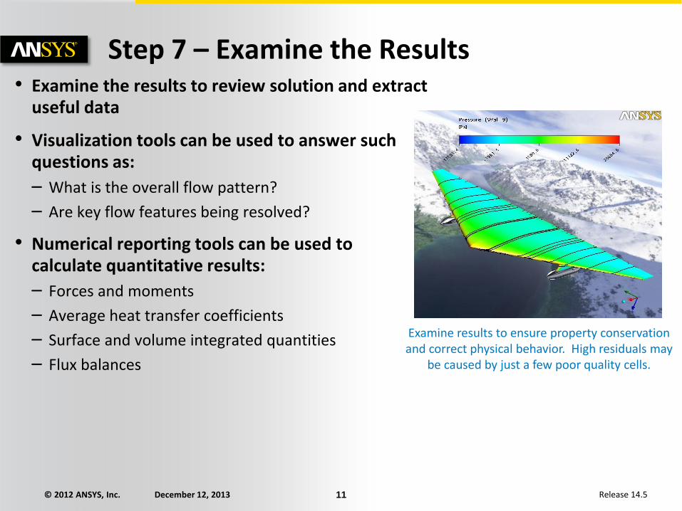
Step 7 – Examine the Results • Examine the results to review solution and extract

useful data

• Visualization tools can be used to answer such questions as:

– What is the overall flow pattern?

– Are key flow features being resolved?

• Numerical reporting tools can be used to calculate quantitative results:

– Forces and moments

– Average heat transfer coefficients

– Surface and volume integrated quantities

– Flux balances

Examine results to ensure property conservation and correct physical behavior. High residuals may

be caused by just a few poor quality cells.


Step 8 – Consider Model Revisions • Are the physical models appropriate?

– Is the flow turbulent?

• Are the boundary conditions correct?

– Is the computational domain large enough?

– Are boundary conditions appropriate?

– Are boundary values reasonable?

• Is the mesh adequate?

– Can the mesh be refined to improve results?

– Does the solution change significantly with a refined mesh, or is the solution mesh independent?

– Does the mesh resolution of the geometry need to be improved?

High residuals may be caused by just a few poor quality cells


Introduction to CFX • The remainder of the lecture will now focus on CFX, covering the following

topics

– Launching CFX, either inside or outside of ANSYS Workbench

– A typical CFD study workflow performed with CFX

– A summary of files and file types


CFX-Pre - Workspace

Outline Tree

Viewer Window

Main Menu

Message Window

Viewer Toolbar

Main Toolbar

CFD-Post CFX-Pre CFX-Solver


CFX-Pre - Workflow

• To define your simulation, generally follow the Outline tree from top to bottom

• Double-click entries in the Outline tree to edit

• Right-click on entries in the Outline tree to insert new items or perform operations

• Some items are optional, depending on your simulation

Mesh and region

control

• Import, delete,

transform meshes

• View & edit mesh

regions

Library objects

• Optional. Referenced elsewhere in the setup

• Import Materials & Reactions from libraries provided

• Insert Expressions, AV’s, Fortran routines

Solver settings

• Convergence controls

• Results files controls

• Numerical schemes

• Monitor points

Initialisation

• Starting point for the

solver in the absence of a

previous solution

Boundary Conditions

Domain

• Right-click to insert

boundary conditions

Analysis Type

• Steady State /

Transient

CFD-Post CFX-

Pre

CFX-

Solver


CFX-Pre – Workflow Example • Load Mesh

– Right-click on ‘Mesh’

A Default Domain is automatically

created when the mesh is imported. It

contains all 3D regions in the mesh.

Every domain contains a default

boundary condition.



CFX-Pre – Workflow Example • Define Domain Properties

– Right-click on the domain and pick Edit

– Or right-click on ‘Flow Analysis 1’ to insert a new domain

When editing an item a new tab panel

opens containing the properties. You

can switch between open tabs.

Sub-tabs contain

various different

properties

Complete the

required fields on

each sub-tab to

define the domain

Optional fields are

activated by

enabling a check

box



CFX-Pre – Workflow Example • Create Boundary Conditions

– Right-click on the domain to insert BC’s


After completing

the boundary

condition, it

appears in the

Outline tree

below its domain


CFX-Pre – Workflow Example • Define Solver Settings

– Right-click on Solver Control and pick Edit


All solver

controls have

default values


CFX-Pre – Workflow Example • Start Solver

– Just close CFX-Pre

• Files are automatically saved

• Check mark shown next to Setup

– Right-click on Solution and select Edit or Refresh

• Refresh runs the solver with default settings

• Edit opens the Solver Manager


Right-click

to solve


CFX Solver Manager • Defining a Run

– CFX-Pre will have written a .def file and this is automatically selected as the Solver Input File

– Can enable Initial Values check box if you have a previous solution to use as the starting point

– Parallel settings are defined here

• Allows you to divide a large CFD problem so that it can run on more than one processor/machine

– Start Run



CFX Solver Manager • Workspace CFD-Post CFX-Pre CFX-Solver

Solution Monitors

• Monitor the convergence of

the solver

• Plot residuals, imbalances,

monitor points, forces,

fluxes…

Text output from the Solver

• Lots of info in here

• Can also view the .out file in

a text editor

Create new monitors


CFX Solver Manager

• When the Solver finishes, start CFD-Post

– Just close the CFX Solver Manager

• Check mark shown next to Solution

– Right-click on Results and select Edit to start CFD-Post


Right-click

to start

CFD-Post


CFD-Post • Workspace CFX-Pre CFD-Post CFX-Solver

Outline Tree

Viewer Window

Details Pane

Outline tree

displays all post-

processing objects.

Right-click or

double-click to edit

in the Details Pane

Editor Tabs • Outline

• Variables

• Expressions

• Calculators


CFD-Post

General Workflow

• Prepare locations where data will be extracted from, or plots generated

– E.g. Planes, Isosurface

• Create variables/expressions which will be used to extract data (if necessary)

– E.g. Drag, pressure ratio

CFX-Pre CFD-Post CFX-Solver

• Generate qualitative data at locations

• Generate quantitative data at locations

• Generate Reports


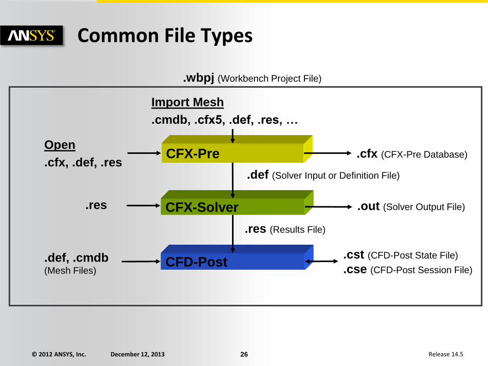
Common File Types

CFX-Solver

CFX-Pre

CFD-Post

.def (Solver Input or Definition File)

.cfx (CFX-Pre Database)

.wbpj (Workbench Project File)

.out (Solver Output File)

.res (Results File)

.cst (CFD-Post State File)

.cse (CFD-Post Session File)

.def, .cmdb (Mesh Files)

Import Mesh

.cmdb, .cfx5, .def, .res, …

Open

.cfx, .def, .res

.res


Workshop 01 – Mixing Tee

• Introductory tutorial for CFX

• Starting from existing mesh – generated in earlier tutorial during the DM / Meshing session

• Model set-up, solution and post-processing

• Mixing of cold and hot water in a T-piece – How well do the fluids mix?

– What are the pressure drops?

Documents

CFD_Pro_14.5_L08_IntroCFD_CFX