Embed Size (px)
Citation preview
1
Title of Thesis
CFD Simulation of Silica Gel and Water Adsorbent
Beds Used in Adsorption Cooling System
By
JOHN WHITE
Student No: 1068698
Project Supervisors: Dr. R. K. Al-Dadah and Dr Michael Ward
A THESIS SUBMITTED
FOR THE DEGREE OF DOCTOR OF PHILOSOPHY
DEPARTMENT OF MECHANICAL ENGINEERING
THE UNIVERSITY OF BIRMINGHAM
2012

University of Birmingham Research Archive
e-theses repository This unpublished thesis/dissertation is copyright of the author and/or third parties. The intellectual property rights of the author or third parties in respect of this work are as defined by The Copyright Designs and Patents Act 1988 or as modified by any successor legislation. Any use made of information contained in this thesis/dissertation must be in accordance with that legislation and must be properly acknowledged. Further distribution or reproduction in any format is prohibited without the permission of the copyright holder.

2
University of Birmingham Research Archive
e-theses repository
This unpublished thesis/dissertation is copyright of the author and/or third parties. The
intellectual property rights of the author or third parties in respect of this work are as defined
by The Copyright Designs and Patents Act 1988 or as modified by any successor legislation.
Any use made of information contained in this thesis must be in accordance with that
legislation and must be properly acknowledged. Further distribution or reproduction in any
format is prohibited without the permission of the copyright holder.
3
ABSTRACT
Adsorption cooling systems are considered to be an important alternative to conventional
heating and cooling systems, however at present it has had limited commercial applications.
This is because of the low thermal heat transfer during its operations cycle from heat
exchanger to adsorbent packing. The main objective of this study is the design and CFD
simulation of a new compact copper wire woven fins heat exchanger and silica gel adsorbent
bed used as part of an adsorption cooling system. This type of heat exchanger has a large
surface area because of the wire woven fins design but can still be design as a small compact
heat exchanger. It is proposed that this will help improve the coefficient of performance
(COP) of the cycle and improve the heat transfer rate in the system. The porous adsorbent
bed is the core component of an adsorption cooling system. Its heat transfer performance has
a control on the adsorption/desorption of vapour refrigerant capacity of the system. The
porous materials used as packing in the adsorbent bed are the fundamental building blocks for
the adsorption cooling system but despite its importance as a packing in an adsorbent bed,
very little is known about flow dynamics in porous media. One reason for this is because of
the difficulty of measuring the heat transfer between porous media and heat exchanger fins,
and adsorption/desorption of water vapour in a full bed. This has restricted the design and
development of this technology, therefore, in order to investigate the heat transfer between
the fins and porous adsorbent, Computational Fluid Dynamics (CFD) Solidworks COSMOS
CFD FLOW Simulation software was used. The software Solidworks COSMOS FLOW
developed by DASSAULT SYSTEMES, has CFD heat transfer, porous material and gas two
phase simulation capability and uses the Finite Volume (FVM) method approach and hybrid
surface modelling method to develop CFD models and assemblies. The software described
are incorporated into Solidworks as add on programs making this CFD programs more users
friendly.
4
This study used flow simulation CFD high resolution to better understand the vapour flow
through complex porous media, adsorbent beds, both sizes of porous media, and arranged and
random sphere packing.
This thesis CFD simulation comprises experimental data derived from using a Dynamic
Vapour Sorption (DVS) adsorption test rig in the Department of Chemical Engineering
University of Birmingham and material published on various types of adsorbent beds,
adsorption cooling systems, technical papers and peer-reviewed journals, leading to the
concept design of an adsorbent bed test rig with a copper wire woven fins heat exchanger.
The purpose for this adsorbent bed design with the use of copper wire woven fins was for two
main reasons:
(i) To help increase the surface area of the heat exchanger without increasing
the size of the heat exchanger.
(ii) To help increase the heat transfer from the heat exchanger to the silica gel
adsorbent which is an associated problem linked to the adsorption cooling
systems low heat transfer.
The wire woven heat exchanger has a larger surface area due to the copper wire woven fins
which help to increase the heat transfer coefficient, enabling it to be used as part of the of an
adsorbent bed.

5
ACKNOWLEDGEMENTS
I would like to thank the following people for their guidance and advice during the course of
this project:
Dr. R. K. Al-Dadah, Project Supervisor, Lecturer in Thermofluids, School of Mechanical
Engineering. University of Birmingham
Dr Michael Ward Senior Lecturer, School of Mechanical Engineering University of
Birmingham.
I would like to acknowledge the advice and assistance of Mr Paul Kerby, Director of P.A.K
Engineering Ltd.
Finally, I wish to express my gratitude to my family and friends for their help and
encouragement, support, understanding and love.
6
Publications
White, J. (2012) “Computational Fluid Dynamics Modelling and Experimental Study on a
Single Silica Gel Type B”, Modelling and Simulation in Engineering, Hindawi Publishing
Corporation. Published online January 2012, vol. 2012, Article ID 598479, 9 pages,
This publication is incorporated as chapter four of this thesis
White, J. (2012) “A CFD Simulation on How the Different Sizes of Silica Gel Will Affect the
Adsorption Performance of Silica Gel”, Modelling and Simulation in Engineering, Hindawi
Publishing Corporation. Published online January 2012 vol. 2012, Article ID 651434, 2
Pages
This publication is incorporated as chapter five of this thesis
White, J and Al-Dadah, R.K. (2012) “The Adaption of Wire Woven Fins to Improve Heat
Transfer and Reduce the Size of Adsorbent Beds”, In Progress
White, J., and Al-Dadah, R.K. (2012) “Using CFD Media Approach to Study Performance in
Adsorbent Beds” In Progress
White, J., and Al-Dadah, R.K (2012) “Compact Adsorbent Bed Design using Wire Woven
Fins”, In Progress
7
TABLE OF CONTENTS
I. ABSTRACT………………………………... 3
II. ACKNOWLEDGEMENTS ……………….. 5
III. PUBLICATION……………………………. 6
IV. TABLE OF CONTENTS ………………….. 7-16
V. LIST OF TABLES ………………………… 17
VI. LIST OF FIGURES………………………... 29
VII. NOMENCLATURE ………………………. 23
Chapter 1
1.1. Introduction……………………………………………………………………………. 26
1.2 Problem statement……………………………………………………………………... 26
1.3 Adsorbent bed modelling………………………………………………………………. 27
1.4 Wire woven fins heat exchanger used as part of the adsorbent bed…………………… 27
1.5 The wire wound fins heat exchanger characteristics…………………………………... 28
1.6 Aims of research……………………………………………………………………….. 28
1.7 Research objectives……………………………………………………………………. 30
1.8. Solving the problem…………………………………………………………………… 30
1.9 Scope of the research…………………………………………………………………... 31
1.10 Research methodology……………………………………………………………….. 31
1.11 Structure of the thesis………………………………………………………………… 32
1.2 Conclusion…………………………………………………………………………….. 34
Chapter 2:
Literature Review
2.1. Introduction……………………………………………………………………………. 35
2.1.1 The adsorption cooling technology………………………………………………….. 36
2.1.2 The main advantages of adsorption cooling technology…………………………….. 36
8
2.1.3 The main disadvantages…………………………………………………………….... 36
2.1.4 Design and development in adsorption cooling technology to date…………………. 37
2.2. The operating principle of an adsorption cooling system……………………………... 42
2.3. Porous adsorbent materials……………………………………………………………. 45
2.3.1 Silica gel……………………………………………………………………………... 45
2.3.2 Zeolite………………………………………………………………………………... 47
2.3.3 Activated carbon……………………………………………………………………... 47
2.4. New types of adsorbents………………………………………………………………. 48
2.4.1. Attapulgite clay adsorbents…………………………………………………………. 49
2.4.2 Silica from micelle template…………………………………………………………. 50
2.4.3 Metal-organic framework adsorbent materials………………………………………. 50
2.5. Types of working adsorbate and adsorbent pairs……………………………………… 51
2.5.1 Silica gel–water………………………………………………………………………. 52
2.5.2 Zeolite-water…………………………………………………………………………. 52
2.6. Principles of adsorption and desorption………………………………………………. 54
2.6.1 Adsorption phenomenon……………………………………………………………... 53
2.6.2 Historical overview of adsorption/desorption……………………………………….. 54
2.6.3 Types of adsorption………………………………………………………………….. 54
2.6.4 Factors affecting desorption…………………………………………………………. 55
2.6.5 Types of adsorption isotherms………………………………………………………. 55
2.6.6 Adsorption equations………………………………………………………………… 58
2.6.7 Adsorption measurement method…………………………………………………… 59
2.6.8 Gas flow method……………………………………………………………………... 60
2.6.9 Gas adsorption volumetric method………………………………………………….. 60
2.6.10. Gas adsorption gravimetry…………………………………………………………. 60
2.7. Enhancement methods used in improving adsorbent bed design……………………... 60
2.7.1. Unconsolidated fixed beds………………………………………………………….. 61
2.7.2 Consolidated adsorbent………………………………………………………………. 62
2.7.3. Coated adsorbents…………………………………………………………………… 63
2.7.4. Direct crystallisation zeolite………………………………………………………… 64
2.8. Conclusion……………………………………………………………………………. 64
9
Chapter 3:
First principles of computational fluid dynamics
Abstract…………………………………………………………………………………….. 66
3.1 Introduction……………………………………………………………………………. 66
3.1.1 History of Computational Fluid Dynamics CFD……………………………………. 66
3.2 CFD governing equations……………………………………………………………… 67
3.3 Turbulence Modelling…………………………………………………………………. 69
3.3.1 The standard κ − ε model……………………………………………………………. 71
3.3.2 The RNG κ − ε model……………………………………………………………….. 71
3.3.3 The realizable κ − ε model…………………………………………………………… 72
3.3.4 Near-wall treatments for wall-bounded turbulent flows……………………………... 73
3.3.5 Flows in Porous Media………………………………………………………………. 73
3.4 CFD Modelling………………………………………………………………………… 77
3.4.1 Computational Fluid Dynamics……………………………………………………… 77
3.4.2 Mesh Specifics in Silica Gel Packed Bed Modelling………………………………... 77
3.5 CFD Mesh Generation…………………………………………………………………. 79
3.5.1 Structured Meshes…………………………………………………………………… 79
3.5.2 Unstructured Meshes………………………………………………………………… 80
3.5.3 Hybrid Meshes………………………………………………………………………. 81
3.6 Commercially Available CFD Method………………………………………………… 81
3.6.1 The finite differences Method (FDM)………………………………………………. 82
3.6.2 Finite Volumes Method (FVM)……………………………………………………… 83
3.6.3 Finite Elements Method (FEM)……………………………………………………… 83
3.6.4 Comparison of the Different CFD Methods…………………………………………. 84
3.7 The three main CFD elements…………………………………………………………. 84
3.7.1 Pre-processing……………………………………………………………………….. 85
3.7.2 Solver………………………………………………………………………………… 86
3.7.3 Post-processing………………………………………………………………………. 86
3.8 CAD Geometry Design………………………………………………………………… 87
3.9 Imposing Boundary Conditions Inlet and Outlet………………………………………. 88
3.10 Using CFD to Validate Experimental data…………………………………………… 88
3.10.1 Experiments vs. CFD Simulations…………………………………………………. 89
3.11 The Computational Fluid Dynamics Software Used in This Thesis…………………. 90
10
3.11.1 The advantages of using CFD……………………………………………………… 90
3.11.2 3 Limitations of CFD ……………………………………………………………… 91
3.12 The Different Types of CFD Simulation Software Package…………………………. 91
3.12.1 Commercial off the Shelf CFD Simulation Software Packages……………………. 92
3.12.2 Custom-built CFD Simulation Specialist Software………………………………… 92
3.12.3 CFD Freeware Software……………………………………………………………. 92
3.13 Conclusion……………………………………………………………………………. 93
Chapter 4:
Computational fluid dynamics modelling and experimental study on a silica gel type B
Abstract…………………………………………………………………………………….. 94
4.1 Introduction…………………………………………………………………………….. 94
4.2 Experimental Apparatus Description…………………………………………………... 96
4.2.1 Experiment Setup and Procedure…………………………………………………….. 97
4.3. GTA Experimental Results……………………………………………………………. 98
4.3.1 The Isotherm Plot for Silica Gel Size 3.5 mm……………………………………….. 99
4.3.2 The Isotherm Plot for Silica Gel Size 5mm………………………………………….. 100
4.3.3 Physical Properties…………………………………………………………………… 101
4.4. CFD model…………………………………………………………………………….. 102
4.4.1 Geometry and Analysis………………………………………………………………. 103
4.4.3 Modelling Of Vapour Flow in a Single Silica Gel Particle………………………….. 104
4.4.4 Porous Media Simulations…………………………………………………………… 104
4.4.5 CFD Porous Medium Methodology…………………………………………………. 104
4.4.6 Model Mesh …………………………………………………………………………. 105
4.4.7 The CFD Mesh Density……………………………………………………………… 106
4.4.8 Simulation Data……………………………………………………………………… 106
4.4.9 Fluid Flow Fundamentals……………………………………………………………. 107
4.5. CFD Results and Discussion………………………………………………………….. 108
4.5.1 Water Vapour Adsorption CFD Simulation…………………………………………. 109
4.5.2 CFD Simulation Of Desorption Of Water Vapour from Silica Gel…………………. 110
4.5.3 Velocity Profiles……………………………………………………………………... 111
4.6. Conclusions……………………………………………………………………………. 112
11
Chapter 5:
A CFD Simulation on how the different sizes of silica gel used in an adsorbent bed will
affect the adsorption performance of silica gel
Abstract…………………………………………………………………………………….. 113
5.1 Introduction…………………………………………………………………………….. 113
5.2 Methods………………………………………………………………………………... 114
5.2.1 3D Geometry of silica gel packing…………………………………………………... 114
5.2.2 Modelling Strategies for Silica Gel Adsorbent Beds……………………………….... 115
5.2.3 Modelling of Vapour Flow in Silica Gel Particle……………………………………. 115
5.3 CFD Governing Equations……………………………………………………………... 118
5.3.1 Desorption of Vapour in Porous Materials…………………………………………... 119
5.4. CFD Modelling Method………………………………………………………………. 120
5.4.1 Smaller Arrangements of Silica Gel Granules……………………………………….. 120
5.4.2. Computational Mesh Domain………………………………………………………. 122
5.4.3 A Porous Sample with Non-uniform Porosity……………………………………….. 122
5.4.4 3D Silica Gel Granules Packing Arrangements……………………………………… 123
5.4.5 CFD Mesh Generation……………………………………………………………….. 123
5.4.6. Porous Media Simulations…………………………………………………………... 124
5.4.7. Porosity of Silica Gel Used in CFD Simulation…………………………………….. 126
5.4.8 Pressure Drop and Mass Transfer…………………………………………………..... 127
5.4.9. Boundary Conditions Used in Simulation…………………………………………... 128
5.4.10. Fluid Flow Fundamentals………………………………………………………….. 129
5.5. Results and Discussion………………………………………………………………... 129
5.5.1. Granules Packing Gap Between Walls……………………………………………… 130
12
5.6. CFD Validation against DVS Experimental………………………………………….. 130
5.6.1 Velocity Profiles……………………………………………………………………... 130
5.6.2. Effect of Flow Velocity……………………………………………………………... 131
5.6.3 The Performance of the Silica Gel…………………………………………………… 132
5.6.4 Water Vapour Flow profile………………………………………………………….. 133
5.6.5. Water Vapour Adsorption profile…………………………………………………… 134
5.6.6. CFD Simulation Of Desorption of Water Vapour from Silica Gel…………………. 134
5.6.7. The Heat Transfer Performance……………………………………………………... 135
5.7 Conclusions…………………………………………………………………………….. 136
Chapter 6
CFD Simulation of two different design configurations of heat exchanger used in
adsorbent bed as part of an adsorption cooling system
Abstract……………………………………………………………………………………...137
6.1. Introduction…………………………………………………………………………..... 137
6.1.1 The Motivation for Heat Transfer Enhancement of the Adsorbent………………….. 138
6.1.2 The heat exchange fin performance………………………………………………….. 139
6.1.3 Common flat plat fin heat exchanger used in a adsorbent bed……………………..... 140
6.1.4 Different type of heat exchanger fin configuration...................................................... 141
6.1.5 Comparison of aluminum flat fins heat exchangers…………………………………. 142
6.2 Equations……………………………………………………………………………… 143
6.3 Heat Transfer in the Two Different Types of Heat Exchangers……………………... 144
6.3.1 The thermal heat transfer of packed beds……………………………………………. 145
6.3.2 Near- Heat Exchanger Fins Wall Small Section Geometries………………………... 145
6.4 Heat Transfer Equations……………………………………………………………….. 146
13
6.5 Results…………………………………………………………………………………. 149
6.5.1 Comparative study…………………………………………………………………… 149
6.6 Experimental Setup and Procedure……………………………………………............. 149
6.7 Computational Fluid Dynamics Simulation ………………………………........……... 152
6.7.1 The Physical Models………………………………………………………………….152
6.7.2 Creating the Silica Gel Porous Medium…………………………………………….. 154
6.7.3 Thermophysical Properties…………………………………………………………... 155
6.8 Surface area and Volume of Flat Fin Results Generated by CFD…………………….. 156
6.8.1 Surface area and Volume of Wire Fin Results Generated by CFD………………….. 160
6.8.2 Wire finned heat exchanger surface area and volume……………………………….. 160
6.9 The Wire Woven Fin Adsorbent Bed………………………………………………… 161
6.9.1 One Pitch of Woven Wire Finned Heat Exchanger ……………………………….. 161
6.9.2 One pitch of wire woven finned heat exchanger with adsorbent packing………….. 163
6.10 Model validation……………………………………………………………………… 164
6.11 Conclusions…………………………………………………………………………… 164
Chapter 7
Scaling up the experimental investigation of a wire woven heat exchanger adsorption
bed pack with silica gel
Abstract…………………………………………………………………………………….. 166
7.1. Introduction……………………………………………………………………………. 166
7.2 Experimental Set-Up…………………………………………………………………... 167
7.2.1 Components………………………………………………………………………….. 167
7.3 Heat Transfer Coefficients and Performance Modelling………………………………. 168
7.4 Wire Wound Finned Tubes…………………………………………………………... 170
7.5 System Measuring Instruments and Measuring Points………………………………... 172
14
7.5.1 Geometries of the Wire Fins and Thermocouples Location…………………………. 172
7.5.2 Temperatures………………………………………………………………………….173
7.5.3 Temperature Sensors…………………………………………………………………. 173
7.5.4 Pressure Vacuum Gauge and Solenoid Valves………………………………………. 173
7.4.5 Flow Meters…………………………………………………………………………. 173
7.5.6 The Data Logger…………………………………………………………………….. 174
7.5.7 Vacuum Pumps………………………………………………………………………. 174
7.6 Wire Woven Fins Heat Exchanger Adsorption Test Rig…………………………….. 174
7.6.1 Testing Procedure……………………………………………………………………. 175
7.6.2 Considerations and Assumptions……………………………………………………. 177
7.6.3 Adsorption Cooling System Simulation Stages……………………………………. 178
7.7 Result and Discussion………………………………………………………………….. 178
7.7.1 Analysis under the Standard Operating Condition…………………………………... 178
7.8 Validation of CFD Simulation Model…………………………………………………..183
7.9 Conclusion……………………………………………………………………………. 184
Chapter 8
8.1 Introduction…………………………………………………………………………….. 185
8.2 Conclusions…………………………………………………………………………….. 185
8.3 Suggestions for Further Work………………………………………………………….. 186
APPENDICES
A. SILICA GEL DATA
B. 25°C TO 85°C ISOTHERMS
15
I hereby declare that all information in this document has been obtained and presented in
accordance with academic rules and ethical conduct. I also declare that, as required by these
rules and conduct, I have fully cited and referenced all material and results that are not
original to this work.
Name, Last name: John White ……………………………….
Signature ………………………………..
Date ………………………………..
16
LIST OF TABLES
Chapter 2
Table 2.1 working pair for adsorption systems…………………………………………….. 51
Chapter 3
Table 3.1 Experiments vs. CFD simulation………………………………………………... 89
Table 3.2 Experiments vs. CFD simulation………………………………………………... 90
Chapter 4
Table 4.1 Thermophysical Properties……………………………………………………… 102
Table 4.2 Thermophysical Properties Used in CFD simulation…………………………… 105
Chapter 5
Table.5.1 Geometry and mesh parameters…………………………………………………. 122
Table.5.2 Thermophysical properties of silica gel…………………………………………. 127
Table 5.3 shows the pressure drop…………………………………………………………. 128
Chapter 6
Table 6.1 thermal conductivity…………………………………………………………...... 143
Table 6.2 shows the heat exchanger heat transfer efficiency………………………………. 151
Table 6.3 Thermophysical properties of copper tube……………………………………… 155
Table 6.4 Thermo-physical properties of silica gel……………………………………....... 156
Table 6.5 Thermo-physical properties of alumina fins…………………………………….. 156
Chapter 7
Table 7.1.Specification for the Copper wire woven fins…………………………………... 170

17
Table 7.2 Parameter of the standard operating condition …………………………………. 177
Table 7.3 Temperature Data……………………………………………………………….. 180
Table.7.4 Temperature Data……………………………………………………………….. 181
Table 7.5 Temperature Data……………………………………………………………….. 182
18
LIST OF FIGURES
Chapter 2
Figure.2.1 Nishiyodo Kuchou Manufacturing Company………………………………….. 37
Figure 2.2 active carbon/methanol adsorption cooling system…………………………… 39
Figure 2.3 Photograph of silica gel–water adsorption chillier……………………………. 40
Figure 2.4 Photograph of experimental facility……………………………………………. 41
Figure.2.5 (a) Heat exchanger surface coated with silica gel using epoxy resin…………... 42
Figure 2.6 Operating Cycle of the adsorption cooling system……………………………...44
Figure 2.7 the common porous adsorbents used as packing in an adsorption bed………… 45
Figure 2.8 the isotherm adsorption curves of silica gel type A, B and C………………….. 46
Figure 2.9 Crystal cell unit of zeolite…………………………………………………….. 47
Figure 2.10 Structure of activated carbon…………………………………………………. 48
Figure 2.11 Attapulgite clay materials…………………………………………………….. 49
Figure 2.12 General Concept for synthesis of mesoporous silica from micelle template…. 50
Figure 2.13 Metal–organic framework adsorbent materials……………………………….. 51
Figure 2.14 the six main types of isotherms……………………………………………….. 56
Figure 2.15 the BET adsorption multi-layer……………………………………………….. 58
Figure 2.16 example of an unconsolidated fixes bed……………………………………… 61
Figure 2.17 Consolidated adsorbent onto tube…………………………………………….. 62
Figure 2.18 SorTech AG……………………………………………………….................. 63
Figure 2.19 photo of a silica gel coated tube………………………………………………. 63
Figure 2.20 direct crystallization with zeolite……………………………………………… 64
19
Chapter 3
Figure 3.1 (a) Silica gel mesh resolution low……………………………………………… 70
Figure 3.2 3D dimensional display and detail of the control volumes……………………. 78
Figure 3.3 Mesh element types for CFD analysis………………………………………….. 79
Figure 3.4 Structured meshes (a) 2D mesh (b) 3D mesh……………………………………80
Figure 3.5 Unstructured meshes (a) 2D mesh (b) 3D mesh…………………………………80
Figure 3.6 Cartesian hybrid meshes…………………………………………………………81
Figure 3.7 illustration of a two dimensional equally distributed mesh……………………...82
Figure 3.8 (a) Mesh and dual mesh of cell FVM (b) Mesh and dual mesh of vertex FVM...83
Figure 3.9 Two-dimensional region subdivided in finite elements………………………….84
Figure 3.10 the inter connectivity functions of the three main elements……………………85
Figure 3.11 establishing by setting the iteration parameters………………………………. .88
Chapter 4
Figure 4.1 pictorial view of the used DVS instrument…………………………………….. 96
Figure 4.2 Schematic of the (DVS) instrument……………………………………………. 97
Figure 4.3 sample container suspended on an extension wire…………………………….. 97
Figure 4.4 One silica gel size 3.5mm type B………………………………………………. 98
Figure.4.5 Moisture sorption behaviour of silica gel type B………………………………. 99
Figure 4.6 Moisture sorption behaviour…………………………………………………….101
Figure 4.7 One silica gel in tube geometry………………………………………………… 104
Figure 4.8 Adsorption and desorption curves……………………………………………… 108
Figure 4.9 Adsorption and desorption curves for silica gel granules size 5mm…………… 109
Figure 4.10 simulation of water vapour adsorption on porous silica gel………………….. 110
20
Figure 4.11 simulation of water vapour desorption………………………………………... 111
Figure 4.12 Velocity vectors profile vector plot of the water vapour……………………… 111
Chapter 5
Figure 5.1 one silica gel in tube geometry…………………………………………………. 116
Figure 5.2 this one granule was then cloned to 36 granules 65 and 114 granules…………. 116
Figure 5.3 thousands of granules pack the silica gel into a 3D adsorption bed……………. 120
Figure 5.4 the three adsorption bed tube…………………………………………………… 121
Figure 5.5 Schematic diagram of the computational domain……………………………… 122
Figure 5.6 arrangements of the silica gel particles for CFD simulation…………………… 123
Figure 5.7 3D dimensional display and detail of the control volumes…………………...... 124
Figure 5.8 CFD Engineering Database……………………………………………….......... 125
Figure 5.9 a typical domain of a porous medium two phase problem…………………….. 126
Figure 5.10 Flow profile in an adsorbent test beds………………………………………… 128
Figure 5.11 Velocity vectors profile in an axial cut model…………………………………131
Figure 5.12 Influence of the silica gel size………………………………………………… 132
Figure 5.13 the adsorption starting to take place with the formation of multilayer………...133
Figure 5.15 concentration profiles…………………………………………………………. 134
Figures 5.16 desorption of water vapour in porous materials……………………………… 135
Figure 5.17 the variation of the surface temperature of silica gel size…………………….. 136
Chapter 6
Figure 6.1 common type of flat fin heat exchanger………………………………………... 140
Figure 6.2 some of the many varieties of finned tubes…………………………………...... 141
Figure 6.3 Different heat transfers…………………………………………………………. 144
Figure 6.4 Heat Exchanger Test Rig……………………………….................................... 149
Figure 6.5 setting up wire fin for heat transfer experiment………………………………... 150
21
Figure 6.6 Setting up Wire Fin for Heat Transfer………………………………………… 151
Figure.6.7 CFD porous adsorbent simulation methodology……………………………...... 153
Figure.6. 8 Define the Engineering Goal…………………………………………………... 154
Figure.6.9 Creating the Silica Gel Porous Medium in CFD……………………………… 154
Figure.6.10 drawing dimension for aluminium…………………………………………..... 157
Figure 6.11 Single flat fin volume…………………………………………………………. 157
Figure 6.12 Aluminium flat plat finned……………………………………………………. 158
Figure 6.13 the contour thermal heat transfer temperature ……………………………….. 159
Figure 6.14 changes of fin heat transfer efficiency over time............................................. 159
Figure 6.15 drawing dimension for copper wire woven finned……………………………. 160
Figure 6.16 One wire woven fin volume and surface………………………………………160
Figure 6.17 3D model of the wire fin without silica gel…………………………………… 161
Figure 6.18 nodes 187365 and elements 86483……………………………………………. 162
Figure 6.19 CFD representations showing a mesh detail…………………………………...162
Figure 6.20 displays the heat transfer efficiency of the wire fin……………………………163
Figure 6.21 changes of fin heat transfer efficiency over time………………………………163
Chapter 7
Figure.7.1 Schematic view of the adsorption cooling test rig …………………………….. 168
Figure 7.2 Wire woven heat exchanger being prepared…………………………………….171
Figure 7.3 (d),(e) wire aluminium mesh was used to cover epoxy attach silica gel……….. 171
Figure 7.4 The location of the thermocouples used to investigation………………………..172
Figure 7.5 the adsorption test rig …………………………………………...……... ……... 175
Figure 7.6 Helix copper coil heat exchanger ……………………………………… ……... 176
Figure 7.7 3D model of test rig …………………………………………………………… 178
Figure 7.8 the refrigerant temperature in the evaporator …………………………………. 179
22
Figure 7.9 the refrigerant temperature in the condenser …………... ………………………179
Figure 7.10 comparison of the outlet temperature between the CFD simulation………….. 180
Figure 7.11 comparison of the outlet temperature between the CFD simulation………….. 181
Figure 7.12 Comparison of the outlet temperature between the CFD simulation………..... 182
Chapter 8
Figure 8.1 design of Concept Design of adsorption cooling system……………………….192
Figure 8.1 Schematic illustration of the adsorption cooling system……………………….192
23
Nomenclature
a : Surface area of silica gel (m2)
C0 : Inlet concentration (kg m-3
)
C : Bed concentration (kg m-3
)
C2 : Inertia resistance coefficient (m)
cp : Specific heat (kJ kg-1
K-1
)
COP : Coefficient of performance (-)
D : Molecular diffusivity (m2 sec
-1)
Dp : Particle diameter (m)
De : efficient water diffusivity (m2/s)
hm : Surface mass transfer coefficient (kg kPa -1
m-2
s-1
)
hfg : Latent heat of vaporisation of water (kJ kg-1
)
Htc : Heat transfer coefficient KW/(m2K)
k : Mass transfer coefficient (sec-1
)
LMTD : Log mean temp difference (°C)
P : Partial pressure (Pa)
Pr : Prandtl number (-)
q : Adsorbent capacity (mmol g-1
)
qs : Maximum capacity (mmol g-1
)
R : Thermal resistance (k/kw)
Rcont : Contact thermal resistance (k/kw)
SCP : Specific cooling power (kw/kg)
24
t : Time (sec)
: The tortuosity factor (-)
u : Water vapour velocity (x-direction) (m sec-1
)
U : Heat loss coefficient (w/m2
°C)
v : Water vapour velocity (y-direction) (m sec-1
)
w : Water vapour velocity (z-direction) (m sec-1
)
wl : Weight loss percentage (w/w%)
∆H : heat of adsorption (J/mole) (-)
ρ : the fluid density (kg/m3)
α : Linear thermal expanding coefficient (K-1
)
λ : Thermal conductivity (kW m-1
K-1
)
∆x : Distance between nodes (m)
∆m : net flow between nodes (kg s-1
)
: Viscosity (kPa s)
ṁ : total mass flow flux of water vapour (kg/sm2)
Greek symbols
ε : Bed fraction (Porosity)
ρs : Particles Density (kg m-3
)
ρ : Fluid Density (kg m-3
)
α : Viscous resistant coefficient (m-1
)
μ : Fluid Viscosity (Ns m-2
)

25
Abbreviation
CFD : Computational Fluid Dynamics
LDF : Linear Driving Force
UDS : User’s Defined Scalars
UDF : User’s Defined Functions
26
CHAPTER 1
1.1. Introduction
Over the years Computational Fluid Dynamics (CFD) has become a standard simulation tool
for the design, analysis, system performance and analysis of engineering systems concerning
fluid flows [1-7]. This increase has been driven by the progress of computer speed, affordable
systems and the ease of availability of new commercial CFD software leading to the steady
decrease in the costs of CFD simulation compared to prototype experiments [2].
A good understanding and an accurate description of adsorption/desorption, water vapour
velocity flow, heat and mass transfer are necessary for the modelling of adsorbent beds as
part of adsorption cooling systems [3-5]. Accurate modelling of porous adsorbent packed -
beds is difficult, due to the existence of wall effects across the entire radius of the bed, flow
outlet, heat and mass diffusion and complex flow structures generated by the internal
geometry of the porous adsorbent packed region. With new methods such as CFD it is
possible to get an in-depth view of the system [6,8].
1.2 Problem Statement
Adsorbent beds are an essential part of the adsorption cooling system as they are used for the
adsorption/desorption of water vapour from the evaporator chamber with the help of a heat
exchanger and porous adsorbent material [1, 3-7]. To improve the modelling of these systems
a more fundamental understanding of the adsorption/desorption of water vapour on to porous
media and the heat transfer from heat exchanger fins to porous media processes taking place
in an adsorbent bed is required [3-8].
This is an area where (computational fluid dynamics) CFD can give a lot more information;
using CFD we can identify heat transfer and water vapour velocity flow patterns inside the
27
adsorbent bed and look at the effects of silica gel adsorption/desorption of water vapour on
different size silica gel granules used as packing in adsorbent bed [3-7].
Some of these studies of fluid dynamics and heat transfer in adsorbent beds date back to the
early twentieth century Augier .F et al [1]. These early investigations of flow in porous media
packed beds provided mainly bulk information such as pressure drop correlations, Mueller,
G. E [2] predict pressure loss for flow in adsorbent beds.
Rahim and Mohseni [3] used CFD to provide an innovative approach to model and analyse
the local flow and the effect of silica gel size on adsorption performance of a packed bed.
CFD simulation of porous media local flow and heat transfer based on CFD technique has
increasingly been reported in recent years in fields of packed bed flow and heat transfer
modelling [7] CFD simulation is based on fundamental principles of diffusion and
adsorption/desorption of porous materials Murakami et al [4].
1.3 Adsorbent Bed Modelling
When attempting to model an adsorbent bed, it is necessary to have a good understanding of
the packing structure, porous adsorbent granule size, porosity, particle distribution and void
fraction and chemical nature [4]. This is of prime importance when evaluating
adsorption/desorption rates in porous adsorbent packed beds, and vapour flow heat and mass
transport phenomena between porous adsorbents and fins [5].
1.4 Wire Woven Fins Heat Exchanger used as Part of the Adsorbent Bed
Wire woven fins heat exchangers have been extensively used in heating and cooling
applications such as engine oil cooler and air heating system but has not yet been adapted for
the application of adsorption cooling system. This type of heat exchanger can be adapted to
be used as part of the adsorbent bed to help solve the problems adsorption system has with
28
the oversize adsorbent bed. This type of heat exchanger has continuous wire loops and
therefore offers good heat transfer efficiency because of the large surface area made by using
wire fins. The advantage of this type of heat exchanger is that it can be designed as a compact
heat exchanger making the adsorbent bed smaller in size [4].
1.5 The Wire Wound Fins Heat Exchanger Characteristics
1. Good heat transfer enabling the design of a compact heat exchanger unit to be used as
part of an adsorbent bed.
2. The above advantage makes it possible to design a heat exchange smaller in size
compared with any other type of fin tubes.
3. Wire wound fin heat exchanger is made from loops of wire spirally wound over a tube
and soldered throughout the length of the tube giving this type of heat exchanger large
surface area.
Geometrical characteristics of the adsorbent bed (its length and diameter) together with the
packing structure will influence the flow behaviour and also the heat and mass transport
mechanisms. Modelling of an adsorbent bed is a difficult task due to the number of problems
that have to be solved in order to obtain a practical model. Existing models for adsorbent bed
heat transfer lump several transport mechanisms into each effective parameter, causing
simulation models to be not descriptive enough. In the published literature no conformity
concerning transport behaviour in porous adsorbent beds can be reached to date.
1.6 Aims of Research
Using a natural refrigerant for adsorption cooling technology is acknowledged as extremely
important from the stand point of the environment, waste heat or solar adsorption cooling are
methods which makes use of natural refrigerant and porous material. Many studies have been
29
carried out in the past few decades to prove the value of this technology for cooling. These
efforts have inspired this study.
Present research through experimental testing and CFD simulation offers a practical strategy
for the adaptability and utility of an adsorption cooling system. This study involved the
design of a wire woven fins and silica gel pack adsorbent bed and data collection from the
experiments conducted on the test rig. It was concerned with the determination of the
interface of individual components constituting the adsorption test rig, thereby, helping the
assessment of the performance of the complete system. The study involved preparation of
CFD simulation model of the full adsorption cooling test rig and the CFD validation of the
model from test results.
This research was also involved in the conceptual development of new wire woven fins with
silica gel packing for incorporation in the CFD simulation model. The CFD simulation of
adsorption cooling system showed that this new design could have beneficial effects on the
performance of the system.
CFD analysis of wire fin and silica gel allowed micro analysis of the water vapour flow and
heat transfer processes occurring in the adsorption bed. This micro study of the adsorption
bed under adsorption and desorption of water vapour allowed an insight into the physical
process that happens inside an adsorbent bed. The CFD study provided knowledge about the
heat transfer attainable by fins and silica gel packing.
Finally, based on a validated model of the adsorption cooling system suggestions were made
regarding the new design of the adsorption cooling system.
30
1.7 Research Objectives
Having outlined the aims of this study it is possible to state its main objectives as follows:
1. The design of a copper wire woven finned heat exchanger to be used as part of an
adsorbent bed.
2. The use of CFD modeling as a research and design tool in the field of adsorption
cooling system.
3. To suggest additional research issues form this present study.
1.8. Solving the Problem
Adsorption cooling systems which run on thermal heat cycle obtained from renewable
sources could be an environmentally friendly alternative to conventional mechanical
compressor systems, if the size of the heat exchanger could be reduced to a smaller size and
the heat transfer between porous adsorbent and heat exchanger improved [2-3]. It is hoped
that the concept design of the new wire woven fin heat exchanger proposal in the area of
adsorption cooling will eventually be used as a common heat exchanger adsorbent bed
design.
Many studies have been undertaken to evaluate the benefits of flat plate fin heat exchanger
adsorbent bed in the adsorption cooling system. However, very few studies have been done to
examine the wire woven fin heat exchanger [7-8]. There is a lack of experimental and CFD
simulation data concerning the use of wire fins as part of an adsorption cooling system. This
study aims to assess the potential of experimental and CFD simulation of silica gel and wire
fin heat exchangers, used as part of an adsorption cooling system [2,4-8].
31
1.9 Scope of the Research
The aim of this work is to establish and validate CFD simulation methodologies for solving
fluid flow and heat and mass transfer phenomena in three-dimensional models of adsorbent
porous packed beds, and apply this strategy as a design tool for adsorbent bed used in
adsorption cooling systems.
In order to accomplish this aim, the following specific objectives were established at the
beginning of the study:
1. Literature review on adsorbent bed design, development and a revision of previous
simulation strategies and approaches to this type of system.
2. Review of particle-to-fluid heat and mass transfer phenomena using water vapour
fluid and silica gel particles through CFD simulations.
3. Validation of the flow velocity field prediction in an adsorbent porous packed bed
through the comparison of CFD simulations against experimental results obtained
from experimental testing.
4. Validation of temperature fields and heat transfer parameters prediction in an
adsorbent bed as part of an adsorption cooling system through the comparison of CFD
simulations against published data.
1.10 Research Methodology
This thesis CFD simulation is based on three sources of data. These are experimental data
done on a Dynamic Vapour Sorption (DVS) adsorption test rig in the Department of
Chemical Engineering University of Birmingham; a wire woven fins heat exchanger
32
adsorption test rig which was used to generate experimental data for the CFD simulation, and
data from published research material on several adsorbent and adsorption cooling systems.
An experimental adsorption test was done on different size of porous adsorbent. The
experiments gave a good insight into the working of water vapour adsorption of different size
of porous media used as packing in adsorbent bed.
Also, an adsorbent bed test rig was designed with a copper wire woven heat exchanger. The
purpose for this adsorbent bed design was for two main reasons (i) was to help reduce the
size of the heat exchanger as this is one of the main problems of the adsorption cooling
system. (ii) To help increase the heat transfer from the heat exchanger to the silica gel
adsorbent, this is also one of the main problems with heat exchanger used at present. This
type of heat exchanger has a large surface area due to the copper wire woven fins which help
to increase the heat transfer coefficient, enabling the design of a compact heat exchanger unit
to be used as part of an adsorbent bed.
A 3D model was prepared in CFD flow simulation. Prior to simulation of this 3D component
model it was necessary to ensure the reliability of the CFD. Accordingly, a validation study
was carried out, which proved the reliability of the CFD simulation model and encouraged
further use of CFD in the modelling of new concept design of an wire woven fins adsorbent
bed design.
1.11 Structure of the Thesis
This thesis covers design and experimental and CFD simulation studies on adsorption cooling
system. The thesis is divided in nine chapters. These are:
Chapter 1, the present chapter, discusses the background of the research work. It outlines the
factors which led to the start of this investigation. It also summarizes the goal of the research
methodology.
33
Chapter 2 is mainly concerned with the review of relevant research work done in the general
area of adsorption cooling technology. The research works reviewed includes theses written
in the area of adsorption cooling, research articles discussing different aspects such as energy
saving, configuration, economics, components and outlines the fundamentals of adsorption
process with reference to silica gel, an important porous material. In this connection
isotherms of porous materials are discussed in some detail and the adsorption cycle is
described. The theory of adsorption explained in some details as well as the potential of CFD
simulation.
Chapter 3 discusses the fundamentals of computational fluid dynamics.
Chapter 4 gives an account of Dynamic Vapour Sorption (DVS) experimental study and CFD
modelling of on silica gel. The model validation curves and their discussions are also given
here along with the simulation results. This chapter was published online in January 2012.
Chapter 5 provides a detailed CFD (Computational fluid dynamics) analysis of adsorbent
beds and how different sizes of silica gel will affect the adsorption and desorption rate, the
use of Solidworks flow simulation software is also given here. The information obtained from
the CFD analysis about the heat transfer and flow behaviour is discussed in detail. This
Chapter was published online in January 2012.
Chapter 6 CFD simulation comparison study have been carried out on a wire woven copper
coil fin and a flat plat fin heat exchanger comparing the heat transfer performance. The CFD
boundary conditions and properties are taken from experimental test rig data, research papers
and heat transfer text books.
Chapter 7 discusses the experimental work performed on the adsorption cooling test rig. This
chapter begins with the introduction of test rig design, its constituting components and data
34
acquisition system. Performance curves of system components such as the evaporator,
condenser and adsorbent beds are discussed. This chapter also outlines the system behavior
under different operating conditions and a full system CFD simulation.
Chapter 8 discusses the conclusions and suggestions for further work. This includes some
guidelines about using adsorption-cooling system in conjunction with other cooling methods.
1.12 Conclusion
A great deal of research covering all important aspects of the adsorption cooling system has
been undertaken in the past few decades; however a major portion of these studies have been
concerned with the mild climate of Europe, China and North America. Few studies have
been conducted for the hotter climates but now there is an increasing requirement to
investigate the performance of adsorption cooling systems due to the need to conserve energy
and find sustainable alternatives. This requirement has been brought about by increasing
environmental concerns of using fossil fuels.
35
CHAPTER 2
LITERATURE REVIEW
Abstract
The main purpose of this chapter is to provide essential understanding of the solar energy or
waste heat power adsorption cooling systems and to give a useful procedure regarding design
parameters of adsorbent beds used in adsorption cooling. Adsorption cooling technology can
meet the needs for cooling requirements such as air-conditioning and food preservation [9-
13]. They have almost no moving parts and are environmentally friendly. For these reasons
there is a growing interest in the development and use of adsorption cooling technology
owing to their various environmental benefits.
2.1. Introduction
Industrial design and development of adsorption cooling systems started in the 1920s by
using silica gel and sulfur dioxide, Miller [9]. However, because of the new development of
CFC refrigerants and the development of mechanical vapour-compression the adsorption
cooling technology was abandoned until the 1970s when IGT [10] conducted a technical
feasibility study of water vapour adsorption cooling system. However, this technology was
not as popular as the mechanical vapour compression driven cooling system in the 1970s. A
design and development researcher Tchernev 1979 [11] started work on adsorption working
pairs to be used in adsorption cooling systems. This was used for the cooling of vaccines in
developing countries. However, because of this development the interest in this type of
technology started to grow rapidly in the 1980s with many cooling system researchers
worldwide working on a variety of adsorption cooling system. A company called Nishiyodo
Kuchou Manufacturing Company (Japan) in 1986, designed and manufactured the first
36
industrial adsorption cooling system see figure.2.1. Since then, the adsorption chiller has
been used and closely evaluated in a wide area of applications in Japan, Europe and USA
with high initial acceptance.
2.1.1 The Adsorption Cooling Technology
The adsorption cooling technology utilises the physical adsorption process where the
molecules of the water vapour or gas are bound to the surface of the porous adsorbent by
Van-der-Waal forces [9,12-20]. These adsorbents are porous materials like silica-gel, zeolites
and activated carbons. The main structural feature of the porous adsorbent and refrigerant
pair is the amount of adsorbed fluid per unit of dry porous adsorbent.
2.1.2 The Main Advantages of Adsorption Cooling Technology
• It is a robust technology with no risk of crystallization, no danger of damage due to
temperatures.
• The materials used today (zeolite, silica gel) are environmentally friendly
• Very low intrinsic electricity consumption due to the lack of a pump. Electricity is
only required for the switching valves and the control unit.
• Very little moving parts with the potential of low maintenance effort and costs.
• High potential of cost reduction in mass production due to the small number of
individual parts.
2.1.3 The Main Disadvantages are
High requirements for vacuum tightness of the container.
Slightly lower COP than comparable absorption technology.
Cyclic temperature variation in the hydraulic circuits requires careful design of the
external hydraulic circuits.
37
Commercially available machines are expensive and only some suppliers are on the
market.
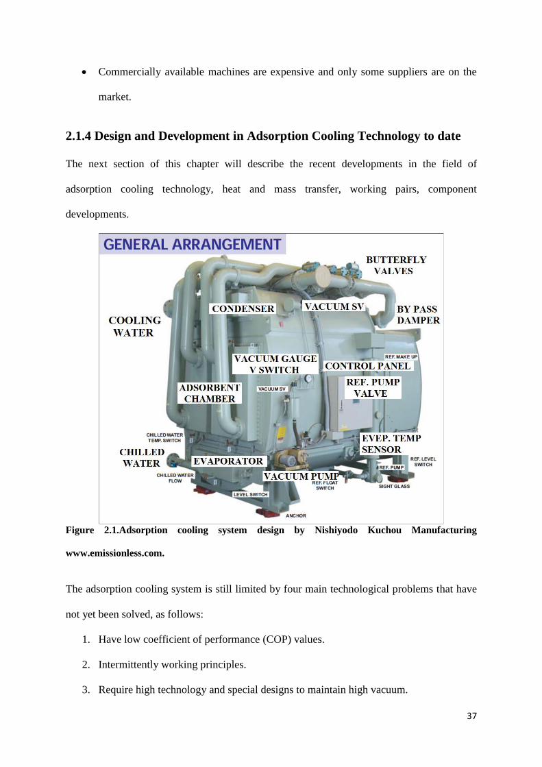
2.1.4 Design and Development in Adsorption Cooling Technology to date
The next section of this chapter will describe the recent developments in the field of
adsorption cooling technology, heat and mass transfer, working pairs, component
developments.
Figure 2.1.Adsorption cooling system design by Nishiyodo Kuchou Manufacturing
www.emissionless.com.
The adsorption cooling system is still limited by four main technological problems that have
not yet been solved, as follows:
1. Have low coefficient of performance (COP) values.
2. Intermittently working principles.
3. Require high technology and special designs to maintain high vacuum.
38
4. Have large volume and weight relative to traditional mechanical heat pump systems.
In the following section of this literature review an attempt is made to give a brief discussion
on the attempts made to design an adsorption cooling system with good coefficient of
performance (COP). Sakoda and Suzuki [13] designed and studied a silica-gal water pair
adsorption cooling system. Sakoda and Suzuki [14] then designed and built a small silica-gal
water cooling system and proposed a simple CFD simulation model which could interpret the
experimental results. Their research showed that the heat transfer area between the porous
adsorbent packed bed and its heat exchanger had a considerable effect on the COP. Gurgel
[15] designed and studied an adsorption cooling drinking fountain using silica gel/water pair.
Cho and Kim [16] designed a tested and developed a CFD simulation code to study the
effects of heat exchangers and heat transfer rate on the cooling capacity of a silica-gal/water
adsorption cooling system. Kluppel and Watabe and Yanadori [17] designed and studied the
cooling characteristic of silica gel /ethanol. Saha et al.[18] studied analytically the
performance of a three-stage silica-gal/water adsorption cooling system to temperatures the
waste heat used was between 55°C to 85°C.
Boelman et al. [19] studied the influence of thermal capacitance and heat exchanger UA-
value on the cooling capacity, power density, and COP of a silica gel-water chillier.
Alam et al. [20] investigated the effect of adsorbent bed on the performance of silica gel
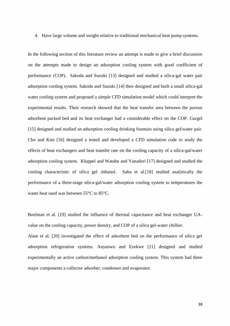
adsorption refrigeration systems. Anyanwu and Ezekwe [21] designed and studied
experimentally an active carbon/methanol adsorption cooling system. This system had three
major components a collector adsorber, condenser and evaporator.
39
The collector was designed as a flat plate type collector adsorber and used clear plane glass
sheet of effective exposed area of 1.2 m2. Connected to steel condenser tube this tube was
immersed in a water tank. The evaporator was designed as a spirally coiled copper tube
immersed in water. Adsorbent cooling during the adsorption process was by solar heat.
According to the study the ambient temperatures during the adsorbate generation and
adsorption process varied over 18.5–34°C.
The refrigerator yielded evaporator temperatures ranging over 1.0–8.5 °C from water initially
in the temperature range 24–28 °C. (See figure.2.2)
Figure 2.2 Active carbon/methanol adsorption cooling system Anyanwu and Ezekwe [21]
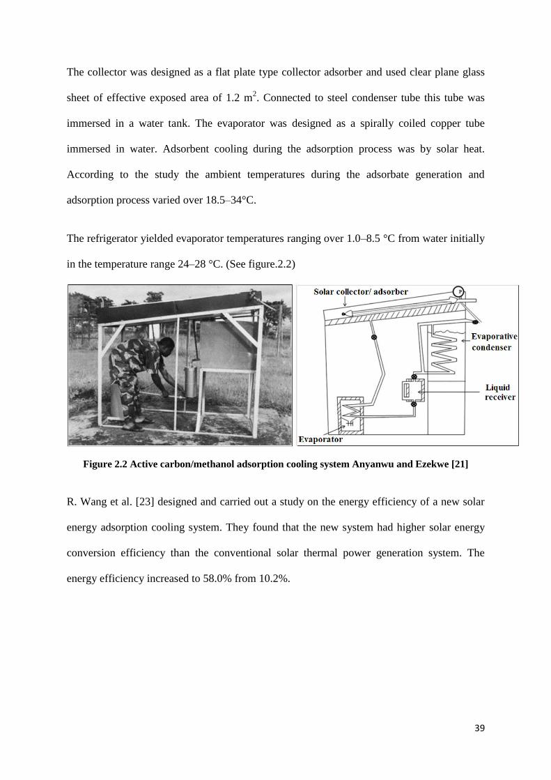
R. Wang et al. [23] designed and carried out a study on the energy efficiency of a new solar
energy adsorption cooling system. They found that the new system had higher solar energy
conversion efficiency than the conventional solar thermal power generation system. The
energy efficiency increased to 58.0% from 10.2%.
40
Figure 2.3 Photograph of silica gel–water adsorption chillier and performance table R. Wang et
al [23].
Anyanwu et al. [24] investigated the effects of the heat transfer of a new heat exchanger
design parameter on the switching frequency, and the results showed that the optimum
switching frequency was very sensitive to the heat exchanger’s design parameters, and
increases with the increase of adsorbent granules packing.
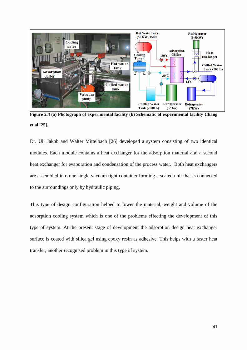
Chang et al [25] designed and tested an adsorption cooling system with silica gel as the
adsorbent and water as the adsorbate. They aimed to reduce the manufacturing costs and
simplify the construction of the adsorption cooling system. A vacuum tank was designed to
contain the adsorption bed and evaporator/condenser. Flat-tube type heat exchangers were
used for adsorption beds in order to increase the heat transfer area and improve the heat
transfer ability between the adsorbent and heat exchanger fins. Under the standard test
conditions of 80°C hot water, 30°C cooling water, and 14°C chilled water inlet temperatures,
a cooling power of 4.3 kW and a coefficient of performance (COP) for cooling of 0.45 were
achieved. It provided a specific cooling power (SCP) of about 176 W/(kg adsorbent). With
lower hot water flow rates, a higher COP of 0.53 was achieved (see figure.2.4).
41
Figure 2.4 (a) Photograph of experimental facility (b) Schematic of experimental facility Chang
et al [25].
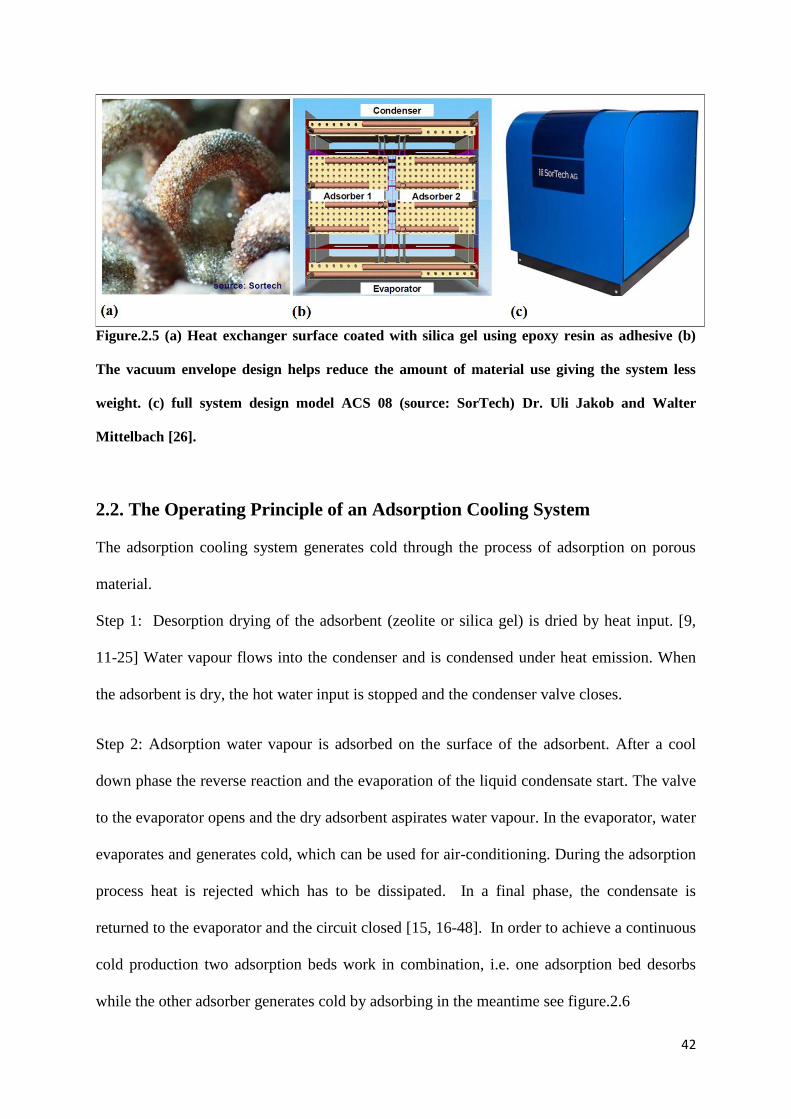
Dr. Uli Jakob and Walter Mittelbach [26] developed a system consisting of two identical
modules. Each module contains a heat exchanger for the adsorption material and a second
heat exchanger for evaporation and condensation of the process water. Both heat exchangers
are assembled into one single vacuum tight container forming a sealed unit that is connected
to the surroundings only by hydraulic piping.
This type of design configuration helped to lower the material, weight and volume of the
adsorption cooling system which is one of the problems effecting the development of this
type of system. At the present stage of development the adsorption design heat exchanger
surface is coated with silica gel using epoxy resin as adhesive. This helps with a faster heat
transfer, another recognised problem in this type of system.
42
Figure.2.5 (a) Heat exchanger surface coated with silica gel using epoxy resin as adhesive (b)
The vacuum envelope design helps reduce the amount of material use giving the system less
weight. (c) full system design model ACS 08 (source: SorTech) Dr. Uli Jakob and Walter
Mittelbach [26].
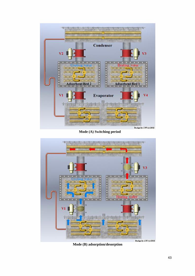
2.2. The Operating Principle of an Adsorption Cooling System
The adsorption cooling system generates cold through the process of adsorption on porous
material.
Step 1: Desorption drying of the adsorbent (zeolite or silica gel) is dried by heat input. [9,
11-25] Water vapour flows into the condenser and is condensed under heat emission. When
the adsorbent is dry, the hot water input is stopped and the condenser valve closes.
Step 2: Adsorption water vapour is adsorbed on the surface of the adsorbent. After a cool
down phase the reverse reaction and the evaporation of the liquid condensate start. The valve
to the evaporator opens and the dry adsorbent aspirates water vapour. In the evaporator, water
evaporates and generates cold, which can be used for air-conditioning. During the adsorption
process heat is rejected which has to be dissipated. In a final phase, the condensate is
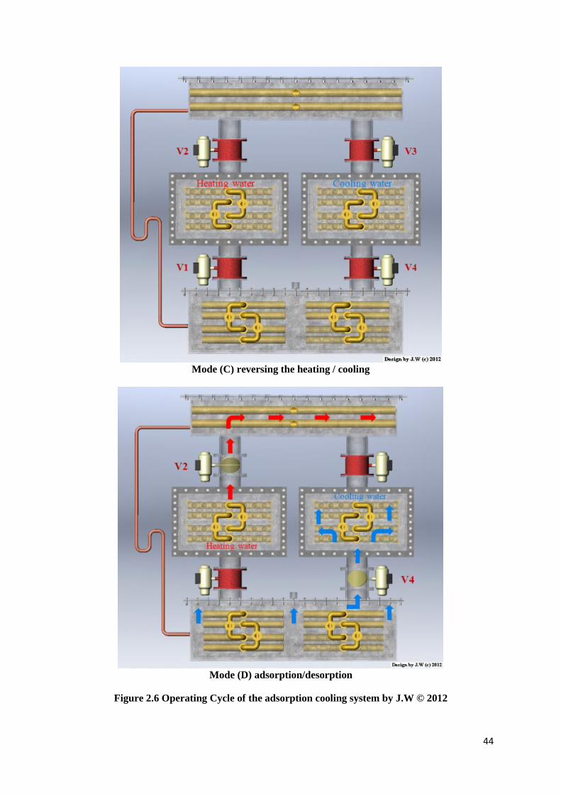
returned to the evaporator and the circuit closed [15, 16-48]. In order to achieve a continuous
cold production two adsorption beds work in combination, i.e. one adsorption bed desorbs
while the other adsorber generates cold by adsorbing in the meantime see figure.2.6
43
Mode (A) Switching period
Mode (B) adsorption/desorption
44
Mode (C) reversing the heating / cooling
Mode (D) adsorption/desorption
Figure 2.6 Operating Cycle of the adsorption cooling system by J.W © 2012
45
2.3. Porous Adsorbent Materials
Almost all porous adsorbents materials have the capacity to adsorb water vapour and gases
by physical and or chemical forces. The porous media materials used on adsorb purpose are
called the adsorbents. The moisture or gases adsorbed can be driven out from the adsorbent
by heating, and the cooled 'dry' adsorbents can adsorb moisture or gases again. The popular
adsorbents are silica-gel, zeolite, and activated carbon [15,16-26].
These porous media materials can be subdivided into 3 categories, set out by IUPAC [27]:
Microporous materials: 0.2–2 nm
Mesoporous materials: 2–50 nm
Macroporous materials: 50–1000 nm
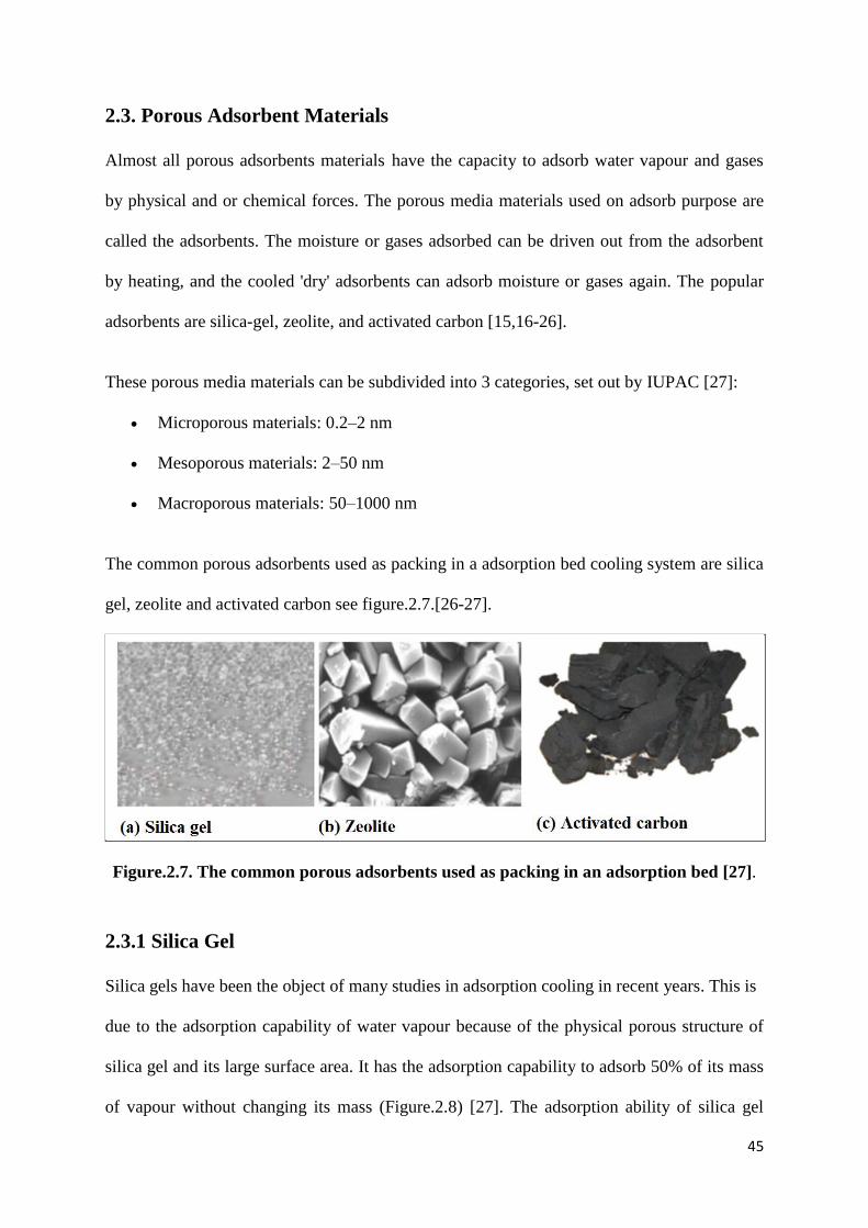
The common porous adsorbents used as packing in a adsorption bed cooling system are silica
gel, zeolite and activated carbon see figure.2.7.[26-27].
Figure.2.7. The common porous adsorbents used as packing in an adsorption bed [27].
2.3.1 Silica Gel
Silica gels have been the object of many studies in adsorption cooling in recent years. This is
due to the adsorption capability of water vapour because of the physical porous structure of
silica gel and its large surface area. It has the adsorption capability to adsorb 50% of its mass
of vapour without changing its mass (Figure.2.8) [27]. The adsorption ability of silica gel
46
increases when the polarity increases. One hydroxyl can adsorb one molecule of water. Each
kind of silica gel has only one type of pore, which usually is confined in narrow channels.
The pore diameters of common silica gel are 2, 3 nm (A type) and 0.7 nm (B type), and the
specific surface area is about 100–1000 m2/g. Type A- silica gel is a fine pore silica gel it has
a large internal surface area [27]. Having a high moisture-adsorbing capacity at low humidity
and is used as an adsorbent in adsorption cooling systems. Type B contains large pores so
type B adsorbs water vapour at low temperature and releases it at high temperature so this
type of silica gel would be more practical for system design to desorbs water vapour at high
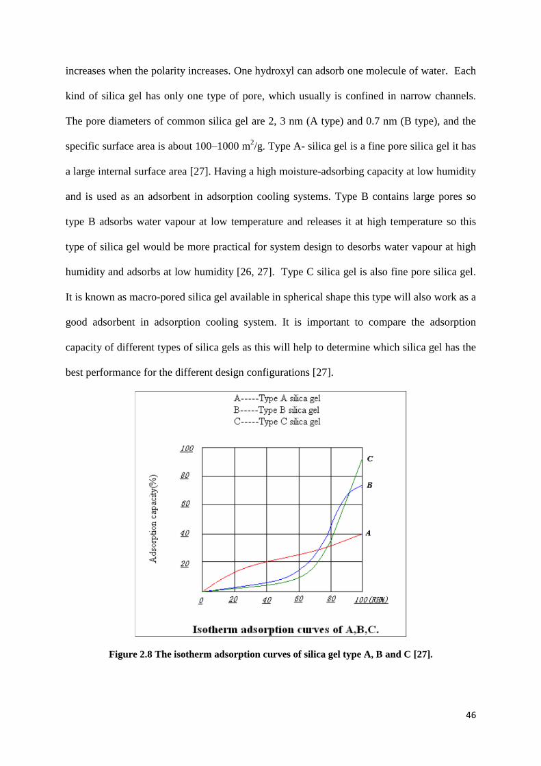
humidity and adsorbs at low humidity [26, 27]. Type C silica gel is also fine pore silica gel.
It is known as macro-pored silica gel available in spherical shape this type will also work as a
good adsorbent in adsorption cooling system. It is important to compare the adsorption
capacity of different types of silica gels as this will help to determine which silica gel has the
best performance for the different design configurations [27].
Figure 2.8 The isotherm adsorption curves of silica gel type A, B and C [27].
47
2.3.2 Zeolite
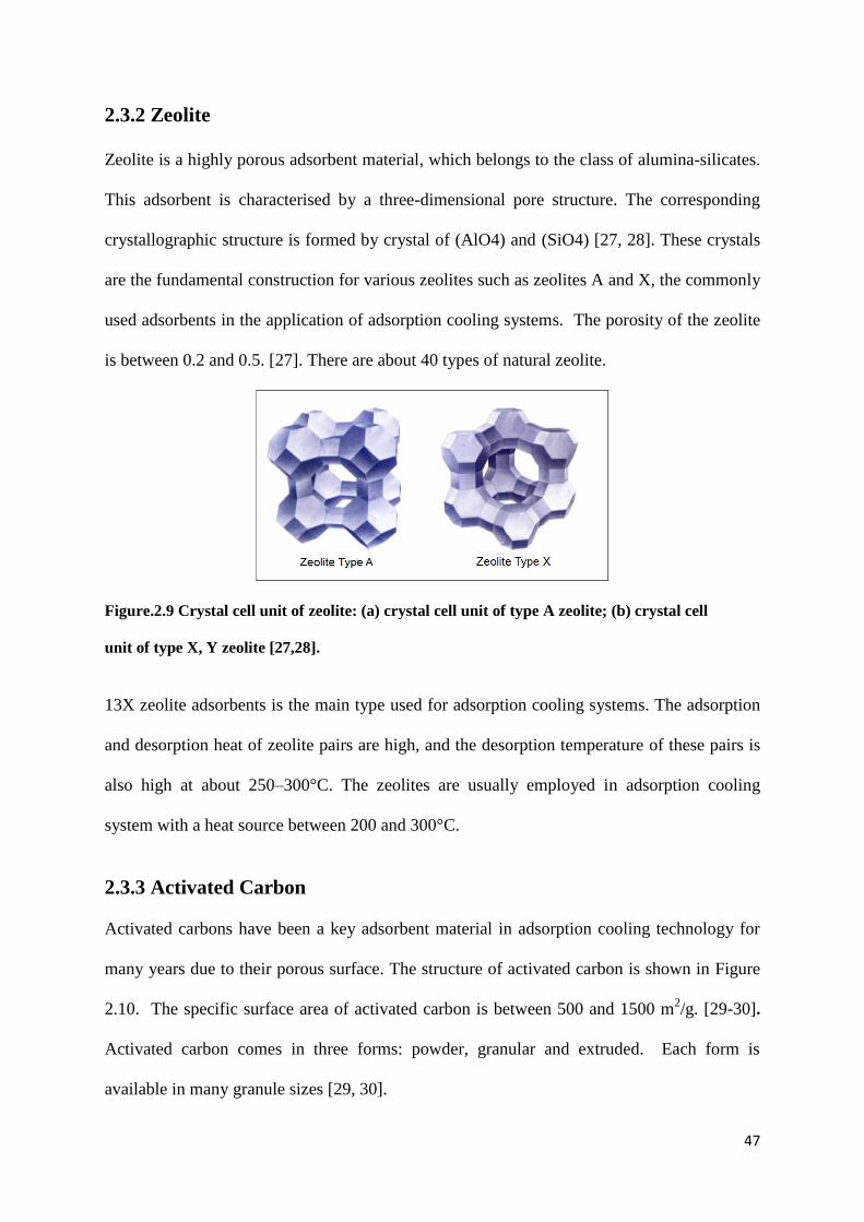
Zeolite is a highly porous adsorbent material, which belongs to the class of alumina-silicates.
This adsorbent is characterised by a three-dimensional pore structure. The corresponding
crystallographic structure is formed by crystal of (AlO4) and (SiO4) [27, 28]. These crystals
are the fundamental construction for various zeolites such as zeolites A and X, the commonly
used adsorbents in the application of adsorption cooling systems. The porosity of the zeolite
is between 0.2 and 0.5. [27]. There are about 40 types of natural zeolite.
Figure.2.9 Crystal cell unit of zeolite: (a) crystal cell unit of type A zeolite; (b) crystal cell
unit of type X, Y zeolite [27,28].
13X zeolite adsorbents is the main type used for adsorption cooling systems. The adsorption
and desorption heat of zeolite pairs are high, and the desorption temperature of these pairs is
also high at about 250–300°C. The zeolites are usually employed in adsorption cooling
system with a heat source between 200 and 300°C.
2.3.3 Activated Carbon
Activated carbons have been a key adsorbent material in adsorption cooling technology for
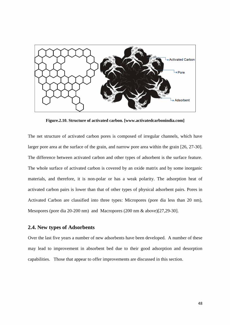
many years due to their porous surface. The structure of activated carbon is shown in Figure
2.10. The specific surface area of activated carbon is between 500 and 1500 m2/g. [29-30].
Activated carbon comes in three forms: powder, granular and extruded. Each form is
available in many granule sizes [29, 30].
48
Figure.2.10. Structure of activated carbon. [www.activatedcarbonindia.com]
The net structure of activated carbon pores is composed of irregular channels, which have
larger pore area at the surface of the grain, and narrow pore area within the grain [26, 27-30].
The difference between activated carbon and other types of adsorbent is the surface feature.
The whole surface of activated carbon is covered by an oxide matrix and by some inorganic
materials, and therefore, it is non-polar or has a weak polarity. The adsorption heat of
activated carbon pairs is lower than that of other types of physical adsorbent pairs. Pores in
Activated Carbon are classified into three types: Micropores (pore dia less than 20 nm),
Mesopores (pore dia 20-200 nm) and Macropores (200 nm & above)[27,29-30].
2.4. New types of Adsorbents
Over the last five years a number of new adsorbents have been developed. A number of these
may lead to improvement in absorbent bed due to their good adsorption and desorption
capabilities. Those that appear to offer improvements are discussed in this section.
49
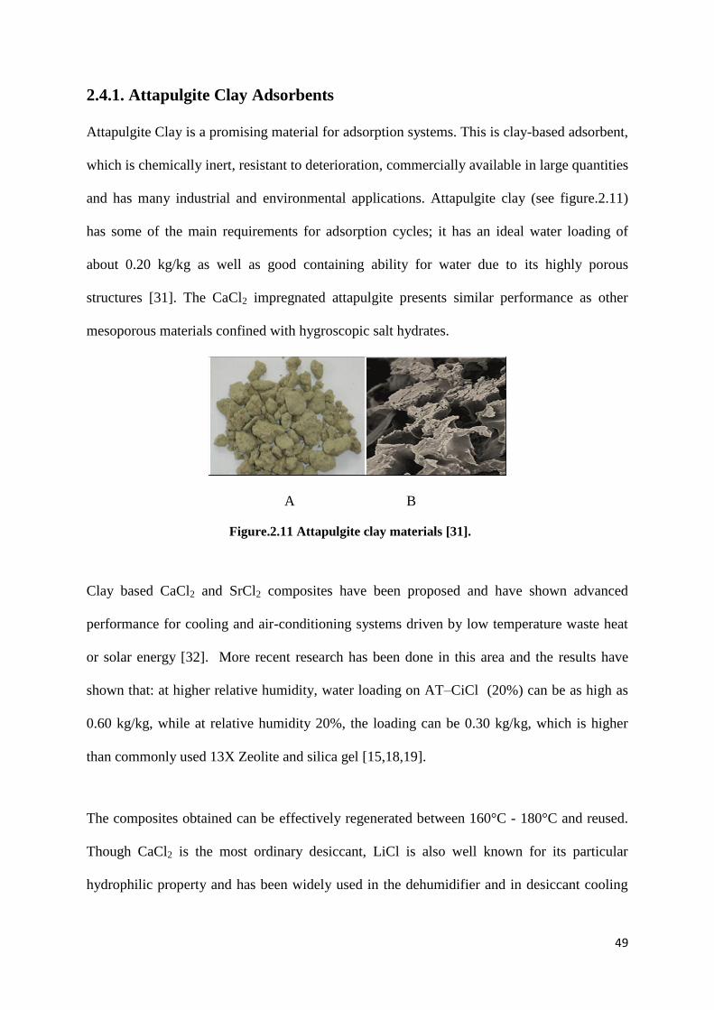
2.4.1. Attapulgite Clay Adsorbents
Attapulgite Clay is a promising material for adsorption systems. This is clay-based adsorbent,
which is chemically inert, resistant to deterioration, commercially available in large quantities
and has many industrial and environmental applications. Attapulgite clay (see figure.2.11)
has some of the main requirements for adsorption cycles; it has an ideal water loading of
about 0.20 kg/kg as well as good containing ability for water due to its highly porous
structures [31]. The CaCl2 impregnated attapulgite presents similar performance as other
mesoporous materials confined with hygroscopic salt hydrates.
A B
Figure.2.11 Attapulgite clay materials [31].
Clay based CaCl2 and SrCl2 composites have been proposed and have shown advanced
performance for cooling and air-conditioning systems driven by low temperature waste heat
or solar energy [32]. More recent research has been done in this area and the results have
shown that: at higher relative humidity, water loading on AT–CiCl (20%) can be as high as
0.60 kg/kg, while at relative humidity 20%, the loading can be 0.30 kg/kg, which is higher
than commonly used 13X Zeolite and silica gel [15,18,19].
The composites obtained can be effectively regenerated between 160°C - 180°C and reused.
Though CaCl2 is the most ordinary desiccant, LiCl is also well known for its particular
hydrophilic property and has been widely used in the dehumidifier and in desiccant cooling
50
systems. Consequently, properties of attapulgite-based LiCl composites deserve closer
investigations.
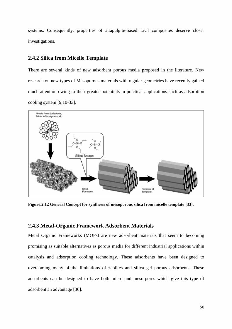
2.4.2 Silica from Micelle Template
There are several kinds of new adsorbent porous media proposed in the literature. New
research on new types of Mesoporous materials with regular geometries have recently gained
much attention owing to their greater potentials in practical applications such as adsorption
cooling system [9,10-33].
Figure.2.12 General Concept for synthesis of mesoporous silica from micelle template [33].
2.4.3 Metal-Organic Framework Adsorbent Materials
Metal Organic Frameworks (MOFs) are new adsorbent materials that seem to becoming
promising as suitable alternatives as porous media for different industrial applications within
catalysis and adsorption cooling technology. These adsorbents have been designed to
overcoming many of the limitations of zeolites and silica gel porous adsorbents. These
adsorbents can be designed to have both micro and meso-pores which give this type of
adsorbent an advantage [36].
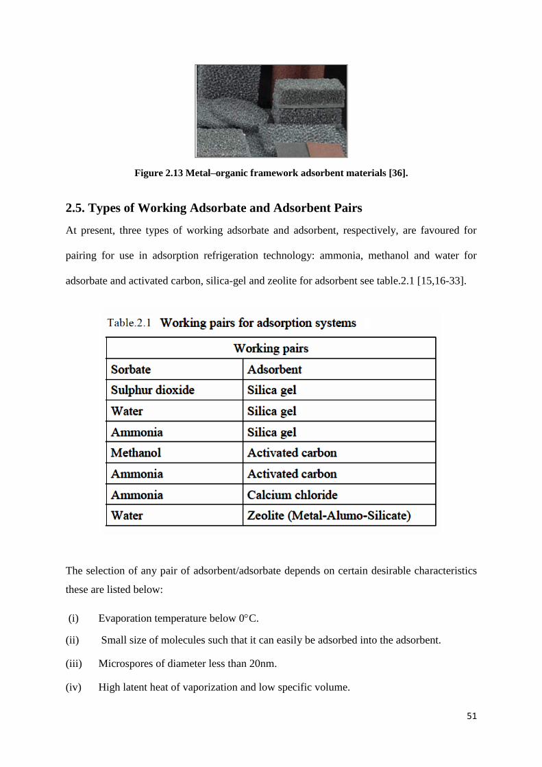
51
Figure 2.13 Metal–organic framework adsorbent materials [36].
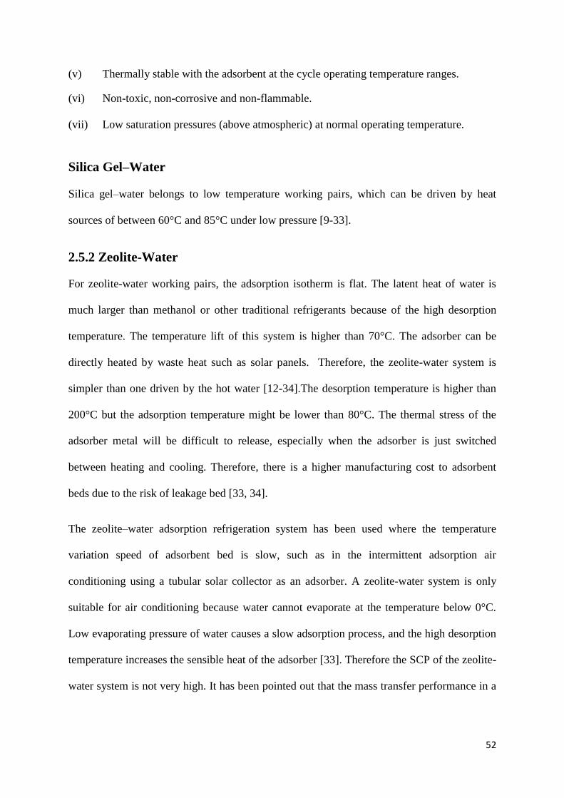
2.5. Types of Working Adsorbate and Adsorbent Pairs
At present, three types of working adsorbate and adsorbent, respectively, are favoured for
pairing for use in adsorption refrigeration technology: ammonia, methanol and water for
adsorbate and activated carbon, silica-gel and zeolite for adsorbent see table.2.1 [15,16-33].
The selection of any pair of adsorbent/adsorbate depends on certain desirable characteristics
these are listed below:
(i) Evaporation temperature below 0C.
(ii) Small size of molecules such that it can easily be adsorbed into the adsorbent.
(iii) Microspores of diameter less than 20nm.
(iv) High latent heat of vaporization and low specific volume.
52
(v) Thermally stable with the adsorbent at the cycle operating temperature ranges.
(vi) Non-toxic, non-corrosive and non-flammable.
(vii) Low saturation pressures (above atmospheric) at normal operating temperature.
Silica Gel–Water
Silica gel–water belongs to low temperature working pairs, which can be driven by heat
sources of between 60°C and 85°C under low pressure [9-33].
2.5.2 Zeolite-Water
For zeolite-water working pairs, the adsorption isotherm is flat. The latent heat of water is
much larger than methanol or other traditional refrigerants because of the high desorption
temperature. The temperature lift of this system is higher than 70°C. The adsorber can be
directly heated by waste heat such as solar panels. Therefore, the zeolite-water system is
simpler than one driven by the hot water [12-34].The desorption temperature is higher than
200°C but the adsorption temperature might be lower than 80°C. The thermal stress of the
adsorber metal will be difficult to release, especially when the adsorber is just switched
between heating and cooling. Therefore, there is a higher manufacturing cost to adsorbent
beds due to the risk of leakage bed [33, 34].
The zeolite–water adsorption refrigeration system has been used where the temperature
variation speed of adsorbent bed is slow, such as in the intermittent adsorption air
conditioning using a tubular solar collector as an adsorber. A zeolite-water system is only
suitable for air conditioning because water cannot evaporate at the temperature below 0°C.
Low evaporating pressure of water causes a slow adsorption process, and the high desorption
temperature increases the sensible heat of the adsorber [33]. Therefore the SCP of the zeolite-
water system is not very high. It has been pointed out that the mass transfer performance in a
53
zeolite-water adsorption refrigeration system is the main factor to influence the improvement
of its performance [9-33].
2.6. Principles of Adsorption and Desorption
The first part of this chapter provides reviews of the different design configuration of
adsorption cooling technology and different adsorbent and adsorbate pairs used in adsorption
cooling technology. This section will serves as an essential background of vapour adsorption
phenomenon before the design and CFD modelling study on this type of system. It aims to
demonstrate the fundamental principles of the adsorption phenomenon which explain the
adsorptions and desorption of water vapour in an adsorption cooling system.
2.6.1 Adsorption Phenomenon
Adsorption phenomenon has fascinated engineers and scientists since the beginning of the
19th century because this phenomenon has been adapted and used in a large number of
technological and extremely important practical applications over the years. Some examples
are in catalytic used in purification of water, sewages, air and adsorption cooling technology.
Despite the developments in this area, scientists are still mystified when it comes to the
phenomenon of adsorption and desorption. One reason for this is that the knowledge and
innovation achieved over time was more through trial and or, rather than through science [9-
22].
The fundamental understanding of the scientific principles of adsorption phenomenon is
underdeveloped, in part, because the study of adsorption of vapour requires extremely careful
experimentation if meaningful results are to be obtained. In recent years substantial effort has
been progressively directed toward closing the gap between practice and theory. Mainly
through the expansion of new approaches by means of CFD computer simulation methods
and owing to new methods which study surface layers. These sections of this review will
54
present, in brief, adsorption and desorption and highlight the theoretical description of the
phenomenon under consideration [16, 34-35].
2.6.2 Historical overview of adsorption/desorption
The phenomenon of adsorption/desorption was discovered over two centuries ago by C. W.
Scheele in 1773 and by the F. Fontana in 1777. In 1785, they found that when they heated
charcoal contained in a test tube it desorbed gases. The gases then adsorbed back when the
charcoal was cooled [37].
The nature of adsorption/desorption has always been a controversial one throughout the
nineteenth century. In a paper Faraday (1834) discussed the possibility that gases are held
onto the surface by an electrical force and suggested that gases could react more easily once
they were in the adsorbed state. However, Berzelius (1836) noted that the best adsorbent was
highly porous materials. Therefore, Berzelius proposed that adsorption was a process where
surface tension or some other force caused gas to be condensed into the pores of a porous
media [37-39].
The idea that most adsorption/desorption processes were really just pore condensations was
actively debated in the literature in the 1850s to 1920s. Magnus (1825, 1853) and Magnus
[1929] showed that pore condensation does occur. However, other investigators found there
were some data that were not in accord with the idea that pore condensation alone explained
adsorption/desorption [37-39].
2.6.3 Types of Adsorption
Types of adsorption will depend upon the vacuum pressure present between vapour or gas
molecules and porous adsorbent, adsorption is classified into two types [12-18]:
55
1. Physical adsorption (Physisorption):
If a force of attraction existing between adsorbate and porous material surface, this is the
Vander Waal’s forces, the adsorption is physical adsorption. In physical adsorption the
attraction between the vapour or gas and porous material surface are weak, hence this type of
adsorption can be easily reversed by heating [15].
2. Chemical adsorption (Chemisorption):
If the forces of attraction existing between vapour or gas and porous material surface have the
same strength as chemical bonds, this type of adsorption is named chemical adsorption. In
chemisorption the force of attraction is strong therefore chemisorption adsorption cannot be
easily reversed [15].
2.6.4 Factors Affecting Adsorption
The rate of adsorption is governed by the following factors [12-17]:
1. Type of adsorbate and adsorbent.
2. The surface area of adsorbent.
3. Experimental conditions.
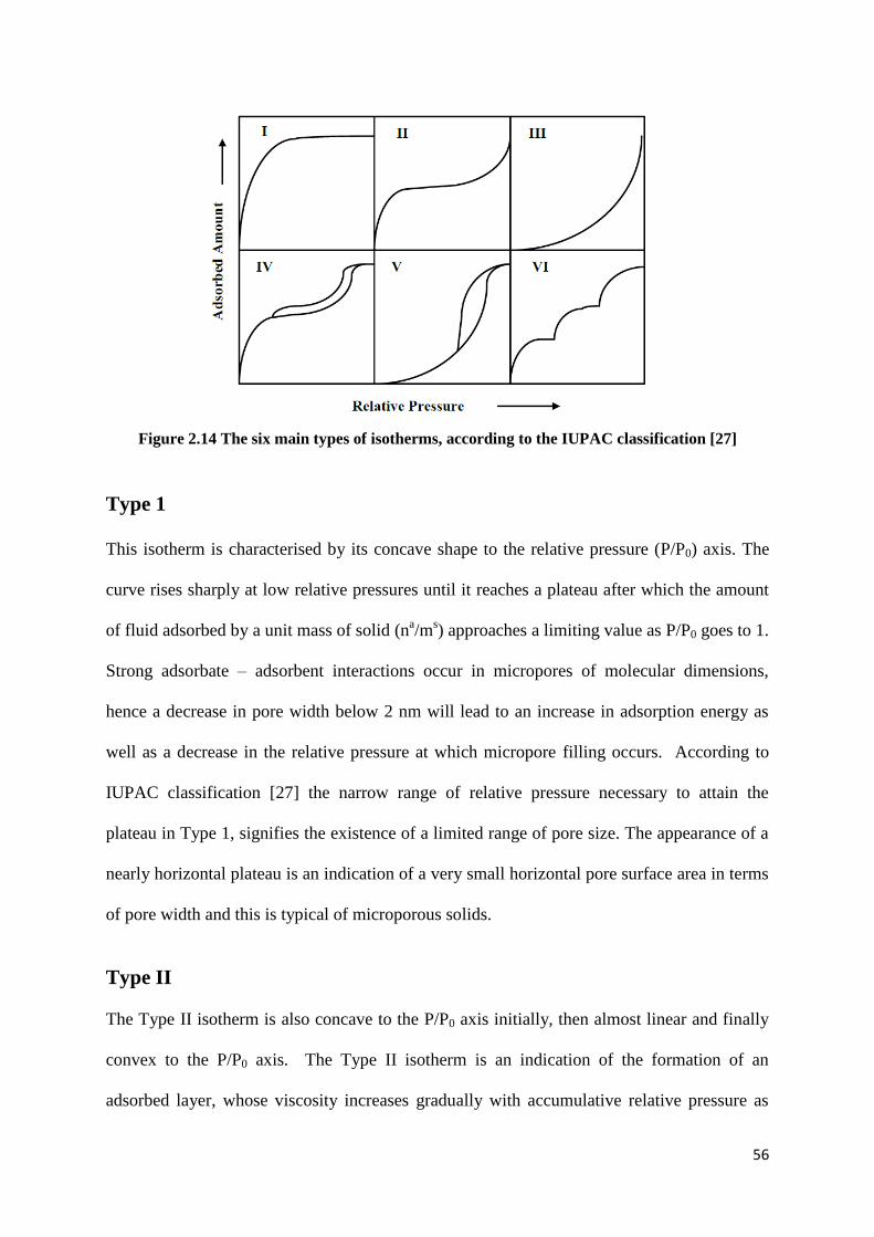
2.6.5 Types of Adsorption Isotherms
Adsorption isotherms measured on a range of gas - solid systems have a variety of forms, and
can be grouped into one of six types according to the International Union of Pure Applied
Chemistry (IUPAC) Classification 1994 [27] with the majority resulting from physisorption,
figure. 2.15 shows the six types of isotherms, which only hold for the adsorption of a single
component gas within its condensable range, and are very useful for the study of porous
materials.
56
Figure 2.14 The six main types of isotherms, according to the IUPAC classification [27]
Type 1
This isotherm is characterised by its concave shape to the relative pressure (P/P0) axis. The
curve rises sharply at low relative pressures until it reaches a plateau after which the amount
of fluid adsorbed by a unit mass of solid (na/m
s) approaches a limiting value as P/P0 goes to 1.
Strong adsorbate – adsorbent interactions occur in micropores of molecular dimensions,
hence a decrease in pore width below 2 nm will lead to an increase in adsorption energy as
well as a decrease in the relative pressure at which micropore filling occurs. According to
IUPAC classification [27] the narrow range of relative pressure necessary to attain the
plateau in Type 1, signifies the existence of a limited range of pore size. The appearance of a
nearly horizontal plateau is an indication of a very small horizontal pore surface area in terms
of pore width and this is typical of microporous solids.
Type II
The Type II isotherm is also concave to the P/P0 axis initially, then almost linear and finally
convex to the P/P0 axis. The Type II isotherm is an indication of the formation of an
adsorbed layer, whose viscosity increases gradually with accumulative relative pressure as
57
P/P0 approaches one layer. Figure 2.15 signifies the completion of a monolayer and the
onset of multilayer adsorption. This point yields an estimate of the amount of adsorbate
required to cover the unit mass of solid surface to a monolayer capacity. Complete
reversibility of the sorption isotherm must be met for normal monolayer-multilayer
adsorption on an open and stable adsorbent. The Type II isotherm is associated with non-
porous and macroporous adsorbents which permits monolayer-multilayer adsorption at high
values of relative pressure (P/P0) [27].
Type III
This is convex to the relative pressure axis, over the whole range. According to Sangwichien
et al [38] this is characteristic of weak adsorbent - adsorbate interactions, and more so, true
Type III isotherms are not common.
Type IV
This isotherm exhibits a similar concave shape to the P/P0 axis as Type II but differs in that it
levels off at high relative pressures. The main characteristic of this isotherm is its incomplete
reversibility. This forms what is known as a hysteresis loop which varies from one system to
another. Hysteresis loops in Type IV isotherms are associated with capillary condensation,
which governs the filling and emptying of pores.
Type V
The Type V isotherm is convex to the P/P0 axis in a similar manner to the Type III, and is
also formed due to weak adsorbent and adsorbate interactions. The main characteristic
difference is that the Type V isotherm exhibits a hysteresis loop which is due to the
mechanism of pour filling and emptying by capillary condensation.
58
Type VI
This has been more recently observed, and is termed the stepped isotherm.
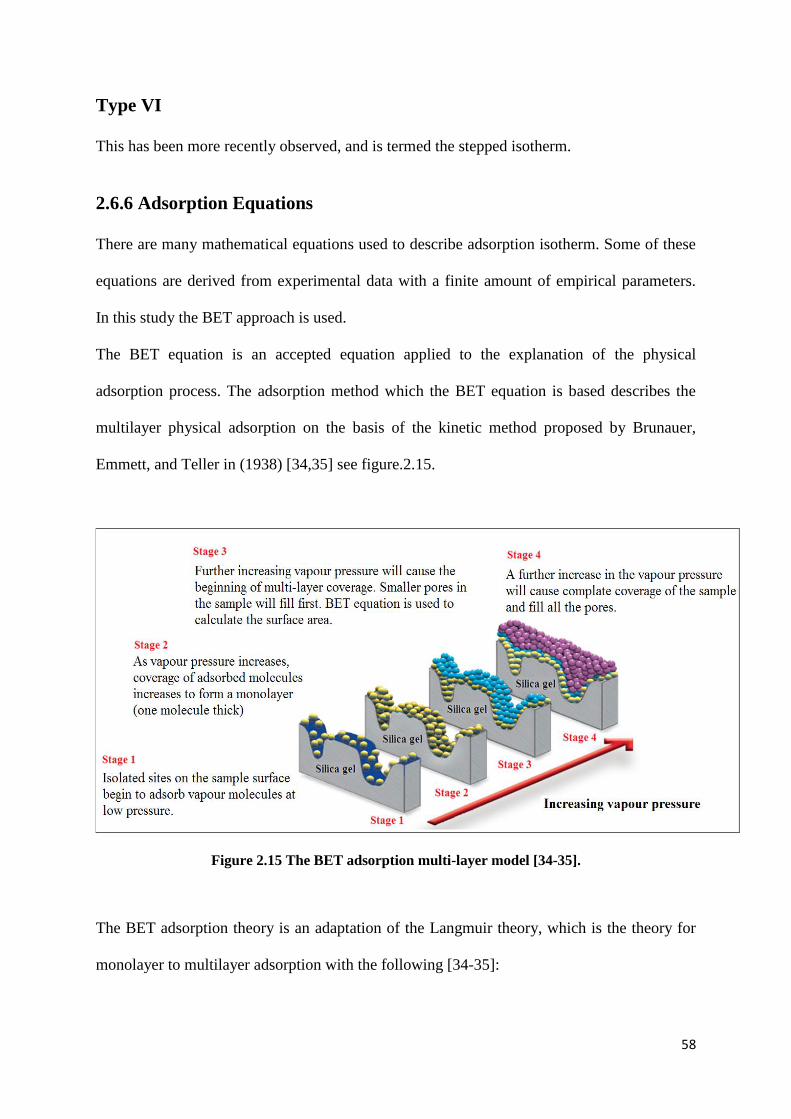
2.6.6 Adsorption Equations
There are many mathematical equations used to describe adsorption isotherm. Some of these
equations are derived from experimental data with a finite amount of empirical parameters.
In this study the BET approach is used.
The BET equation is an accepted equation applied to the explanation of the physical
adsorption process. The adsorption method which the BET equation is based describes the
multilayer physical adsorption on the basis of the kinetic method proposed by Brunauer,
Emmett, and Teller in (1938) [34,35] see figure.2.15.
Figure 2.15 The BET adsorption multi-layer model [34-35].
The BET adsorption theory is an adaptation of the Langmuir theory, which is the theory for
monolayer to multilayer adsorption with the following [34-35]:
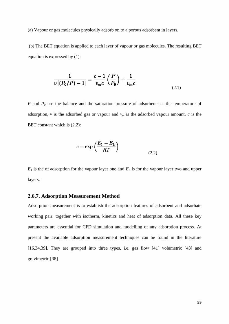
59
(a) Vapour or gas molecules physically adsorb on to a porous adsorbent in layers.
(b) The BET equation is applied to each layer of vapour or gas molecules. The resulting BET
equation is expressed by (1):
(2.1)
P and P0 are the balance and the saturation pressure of adsorbents at the temperature of
adsorption, v is the adsorbed gas or vapour and vm is the adsorbed vapour amount. c is the
BET constant which is (2.2):
(2.2)
E1 is the of adsorption for the vapour layer one and EL is for the vapour layer two and upper
layers.
2.6.7. Adsorption Measurement Method
Adsorption measurement is to establish the adsorption features of adsorbent and adsorbate
working pair, together with isotherm, kinetics and heat of adsorption data. All these key
parameters are essential for CFD simulation and modelling of any adsorption process. At
present the available adsorption measurement techniques can be found in the literature
[16,34,39]. They are grouped into three types, i.e. gas flow [41] volumetric [43] and
gravimetric [38].
60
2.6.8 Gas Flow Method
This type of adsorption measurement method was first proposed by Nelsen and Eggertsen
[41]. This test rig used helium as the transporter gas and a flow meter was used to calculate
the pressure of the vapour or gas. The adsorbed gas volume is determined from the peak area
in the adsorption/desorption chart recorded by a potentiometer over a period of time. This test
rig is inexpensive and easy to operate. However, the measurement of this adsorption method
is not accurate. This method is usually useful for fast single point determinations of the
specific surface area. Multipoint measurements of isotherms need a more accurate method of
measurement in order to be used in CFD simulation.
2.6.9 Gas Adsorption Volumetric Method
The volumetric gas adsorption method was first proposed by Emmett [41], in which the gas
adsorption was measured by a mercury burette and manometer. The quantity of gas adsorbed
was measured by the gas volume change in the burette. However, the mercury burette is no
longer used because of the concerns of element toxicity and has led to mercury burettes being
phased out of use.
Gas Adsorption Gravimetry
In gas adsorption gravimetry, the adsorbed mass, adsorption pressure and temperature are
measured directly and independently. This adsorption method is a more accurate method and
is becoming more popular in the adsorption measurement of silica gel adsorbent [25-38].
2.7. Enhancement Methods Used in Improving Adsorbent Bed Design
The choice of the adsorbent has a significant impact on the performance of adsorption
refrigerators. Detailed reviews about adsorbents and working pairs for heat transformation
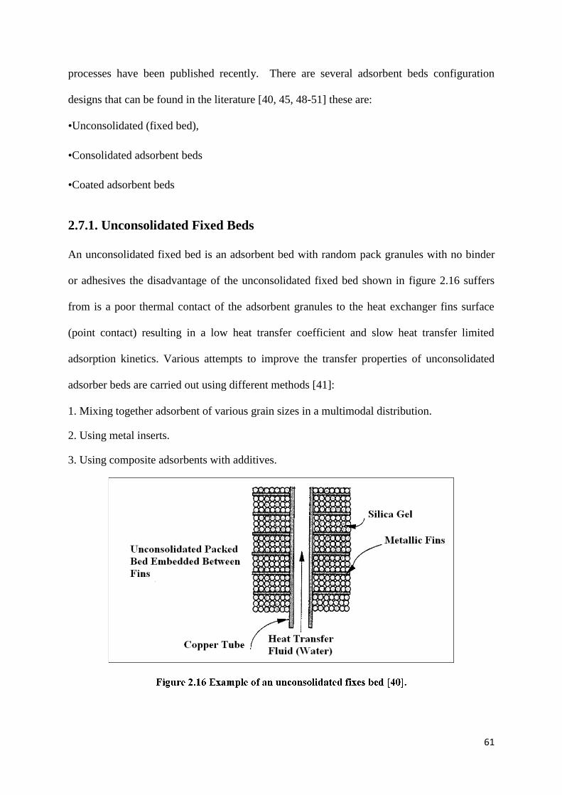
61
processes have been published recently. There are several adsorbent beds configuration
designs that can be found in the literature [40, 45, 48-51] these are:
•Unconsolidated (fixed bed),
•Consolidated adsorbent beds
•Coated adsorbent beds
2.7.1. Unconsolidated Fixed Beds
An unconsolidated fixed bed is an adsorbent bed with random pack granules with no binder
or adhesives the disadvantage of the unconsolidated fixed bed shown in figure 2.16 suffers
from is a poor thermal contact of the adsorbent granules to the heat exchanger fins surface
(point contact) resulting in a low heat transfer coefficient and slow heat transfer limited
adsorption kinetics. Various attempts to improve the transfer properties of unconsolidated
adsorber beds are carried out using different methods [41]:
1. Mixing together adsorbent of various grain sizes in a multimodal distribution.
2. Using metal inserts.
3. Using composite adsorbents with additives.
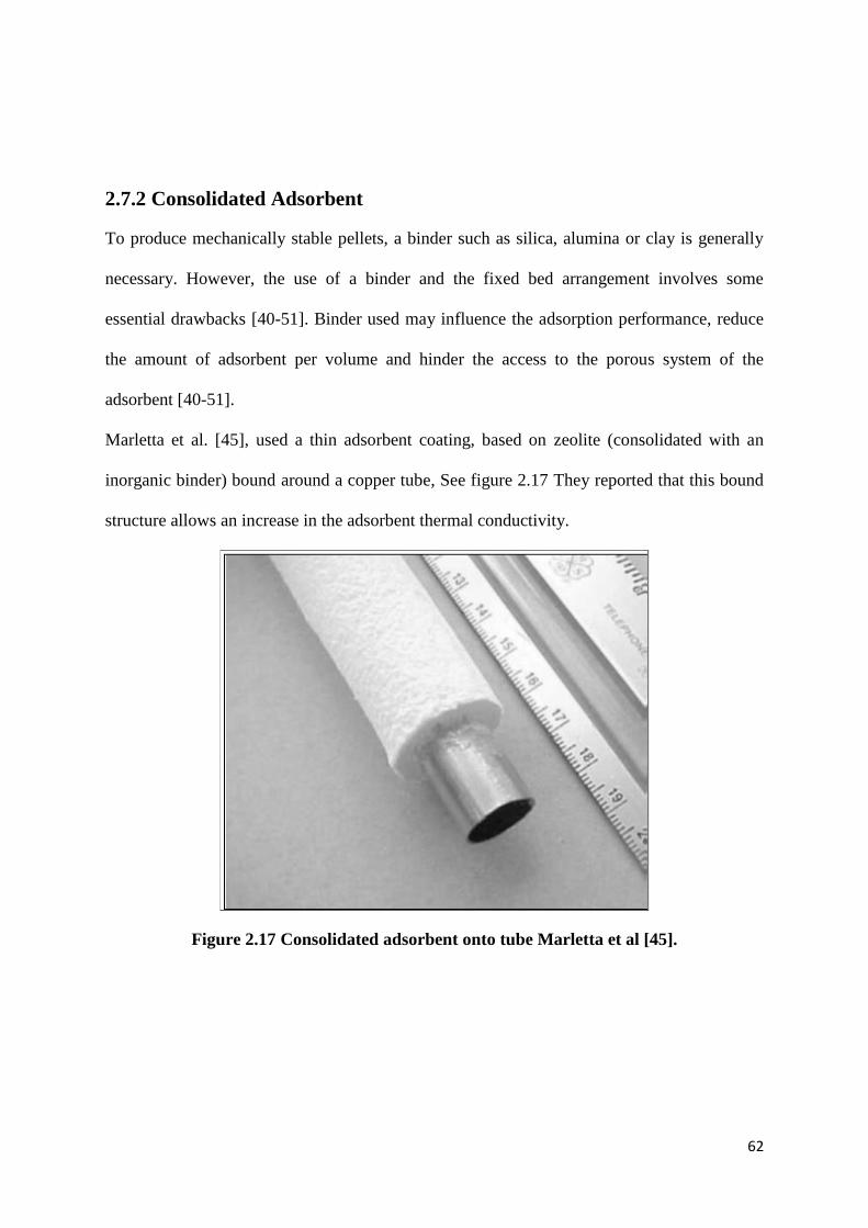
62
2.7.2 Consolidated Adsorbent
To produce mechanically stable pellets, a binder such as silica, alumina or clay is generally
necessary. However, the use of a binder and the fixed bed arrangement involves some
essential drawbacks [40-51]. Binder used may influence the adsorption performance, reduce
the amount of adsorbent per volume and hinder the access to the porous system of the
adsorbent [40-51].
Marletta et al. [45], used a thin adsorbent coating, based on zeolite (consolidated with an
inorganic binder) bound around a copper tube, See figure 2.17 They reported that this bound
structure allows an increase in the adsorbent thermal conductivity.
Figure 2.17 Consolidated adsorbent onto tube Marletta et al [45].
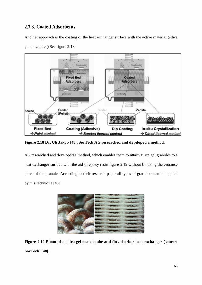
63
2.7.3. Coated Adsorbents
Another approach is the coating of the heat exchanger surface with the active material (silica
gel or zeolites) See figure 2.18
Figure 2.18 Dr. Uli Jakob [48], SorTech AG researched and developed a method.
AG researched and developed a method, which enables them to attach silica gel granules to a
heat exchanger surface with the aid of epoxy resin figure 2.19 without blocking the entrance
pores of the granule. According to their research paper all types of granulate can be applied
by this technique [48].
Figure 2.19 Photo of a silica gel coated tube and fin adsorber heat exchanger (source:
SorTech) [48].
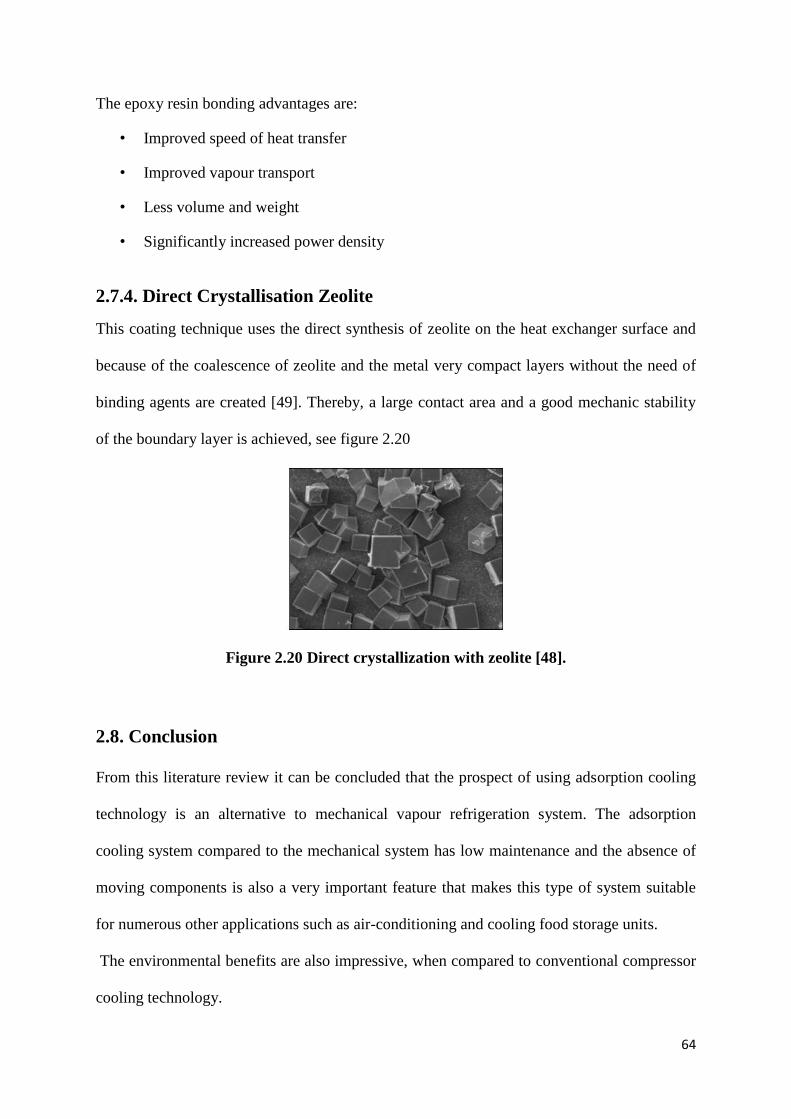
64
The epoxy resin bonding advantages are:
• Improved speed of heat transfer
• Improved vapour transport
• Less volume and weight
• Significantly increased power density
2.7.4. Direct Crystallisation Zeolite
This coating technique uses the direct synthesis of zeolite on the heat exchanger surface and
because of the coalescence of zeolite and the metal very compact layers without the need of
binding agents are created [49]. Thereby, a large contact area and a good mechanic stability
of the boundary layer is achieved, see figure 2.20
Figure 2.20 Direct crystallization with zeolite [48].
2.8. Conclusion
From this literature review it can be concluded that the prospect of using adsorption cooling
technology is an alternative to mechanical vapour refrigeration system. The adsorption
cooling system compared to the mechanical system has low maintenance and the absence of
moving components is also a very important feature that makes this type of system suitable
for numerous other applications such as air-conditioning and cooling food storage units.
The environmental benefits are also impressive, when compared to conventional compressor
cooling technology.
65
The absence of harmful or hazardous products such as CFCs, together with a substantial
reduction of CO2 emissions due to very low consumption of electricity, creates an
environmentally safe technology. Low-temperature waste heat or solar energy can be
converted into a chilling capacity as low as 5°C. However, the adsorption cooling technology
is restricted by the poor thermal conductivity of porous media and large heat exchanger used
in this system. There are two ways one could solve these problems, one is to develop a new
adsorbent material which would have a better adsorption capacity; another, could be to
redesign the construction of the adsorbent bed with the help of CFD modelling in order to
improve the heat transfer to the porous material used as the adsorption packing.
66
CHAPTER 3
FIRST PRINCIPLES OF COMPUTATIONAL FLUID
DYNAMICS Abstract
This chapter focuses on the principles of Computational Fluid Dynamics (CFD), flow
phenomena in porous media, and mathematical models for water vapour and heat transfer
processes in adsorbent bed used in adsorption cooling system. Five areas of relevant literature
were reviewed: (a) general modelling methodology; (b) basic principles of CFD; (c) porous
media approach; (d) modelling of water vapour; (e) modelling of heat transfer in adsorbent
beds.
3.1Introduction
Computational Fluid Dynamics (CFD) is the term given to the task of solving the fluid flow
and governing equations by a computer. However the equations governing fluid flow have
been known for over 100 years major advances in CFD were hindered until the 1970s when
digital computers became accessible to the scientific researchers and the public [53-59]. The
speed of modern computers and relatively low price and the new commercial CFD codes now
accessible makes CFD a very suitable tool for researcher and designers engineers [52].
Currently there are several widely used commercial CFD tools such as COMSOL
MULTIPHYSICS, SolidWorks COSMOS FLOW SIMULATION, PHOENICS, FLUENT,
CFX, and STAR-CD.
3.1.1 History of Computational Fluid Dynamics CFD
In the eighteenth and nineteenth century engineer and mathematicians mathematically
describe the motion of fluids [126]. Daniel Bernoulli derived the famous Bernoulli s equation
(1738) and Leonhard Euler proposed the Euler equations which describes the conservation of
67
momentum for fluid flow, and conservation of mass. He also proposed the velocity potential
theory. Two important contributors to the field of computational fluid dynamics were Claude
Louis Marie Henry Navier and the Irishman, George Gabriel Stokes who introduced viscous
transport into the Euler equations, which resulted in the now famous Navier-Stokes
equations.
These forms of the differential mathematical equations that they proposed nearly 200 years
ago are the foundation of the modern computational fluid dynamics (CFD) simulation
modelling they include expressions for the conservation of mass, momentum, energy and
turbulence. However it was not until the arrival of modern computers in the 1960s and 1970s
that they could be resolved for real flow problems within a reasonable timescales. It was at
this point in time considerable amount of work was carried out on development of the
theories of boundary layers and turbulence in CFD fluid flow.
3.2 CFD governing equations
The fundamental governing equations of fluid dynamics are the mass, momentum and energy
equations as mention above. These three equations are the fundamental principles upon the
computational fluid dynamics are based [76, 77].
• Mass
• Momentum
• Energy
The first law states that mass cannot be created nor destroyed. The second law states that the
rate of change of momentum equals the sum of the forces on a fluid particle, and is described
by Newton’s second law. The third law states that the rate of change of energy is equal to the
rate of change of heat addition and work done on a fluid particle, and is the first law of
thermodynamics. If the motion of a fluid is only affected by phenomena on a macroscopic
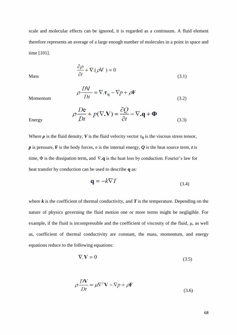
68
scale and molecular effects can be ignored, it is regarded as a continuum. A fluid element
therefore represents an average of a large enough number of molecules in a point in space and
time [101].
Mass (3.1)
Momentum (3.2)
Energy (3.3)
Where ρ is the fluid density, V is the fluid velocity vector τij is the viscous stress tensor,
p is pressure, F is the body forces, e is the internal energy, Q is the heat source term, t is
time, Φ is the dissipation term, and .q is the heat loss by conduction. Fourier’s law for
heat transfer by conduction can be used to describe q as:
(3.4)
where k is the coefficient of thermal conductivity, and T is the temperature. Depending on the
nature of physics governing the fluid motion one or more terms might be negligible. For
example, if the fluid is incompressible and the coefficient of viscosity of the fluid, μ, as well
as, coefficient of thermal conductivity are constant, the mass, momentum, and energy
equations reduce to the following equations:
(3.5)
(3.6)
69
(3.7)
Presence of each term and their combinations determines the appropriate solution numerical
procedure.
3.3 Turbulence Modelling
Water vapour turbulence in an adsorbent bed is a three-dimensional time dependent motion in
which causes vapour velocity variations. Turbulence is one of the most complex phenomena
in an adsorbent bed. Some of the reasons for the complexity are [68]:
1. Intrinsic randomness: Turbulent flows are extremely sensitive to small disturbances
due to which turbulent flows inherently have no repeatability
2. Intermittency: Turbulence can interact with non-turbulent fluid flow and can appear
intermittently in time at certain location.
Although turbulence is a very complex flow phenomenon it can be computed by using the
Reynolds Averaged Navier -Stokes (RANS) methods. This method predicts the flow
perfectly in many simulated circumstances.
Compiling the Navier-Stokes equations into the RANS equations makes it possible to
simulate practical flow simulation in an adsorbent bed. The assumption (known as the
Reynolds decomposition) behind the RANS equations is that the time-dependent turbulent
velocity variations can be separated from the mean flow velocity. This transform then
introduces a set of unknowns called the Reynolds stresses, which are functions of the velocity
variations and which require a turbulence model (e.g. the two-equation k-epsilon model) to
produce a closed system of solvable equations. The reduced computational requirements for
the RANS equations while still significant are orders of magnitude less than that required for
the original Navier-Stokes equations. Another advantage of using the RANS equations for
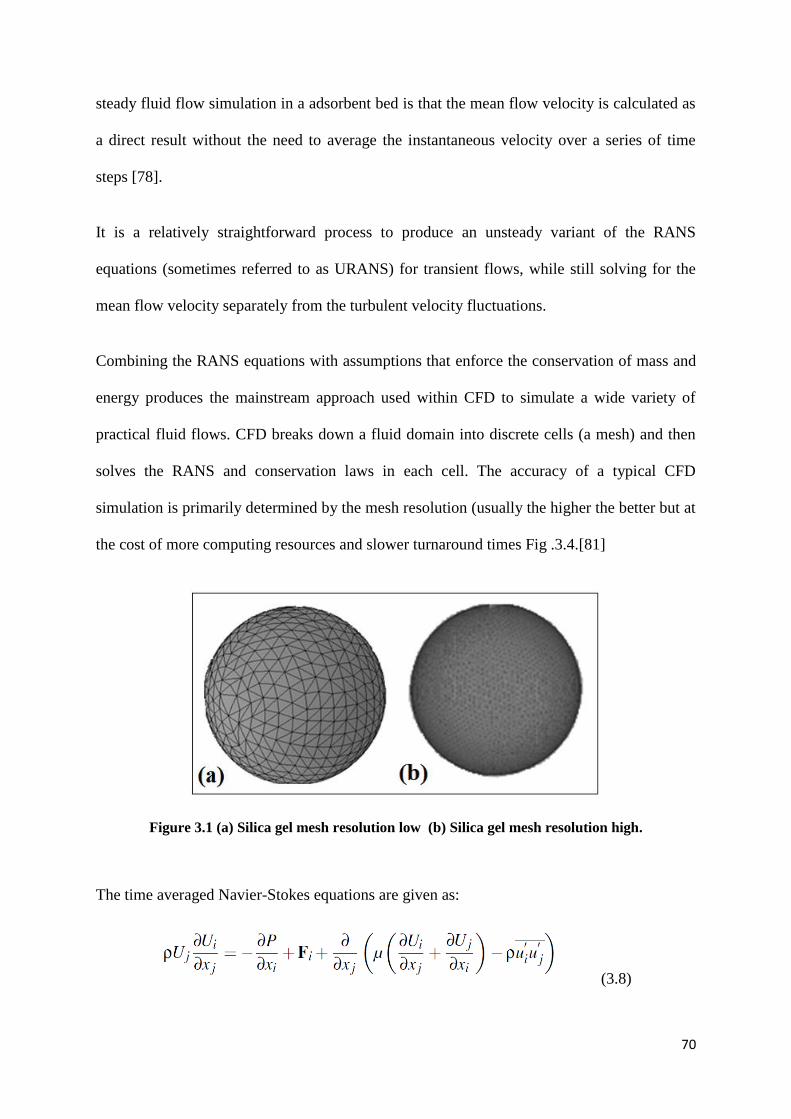
70
steady fluid flow simulation in a adsorbent bed is that the mean flow velocity is calculated as
a direct result without the need to average the instantaneous velocity over a series of time
steps [78].
It is a relatively straightforward process to produce an unsteady variant of the RANS
equations (sometimes referred to as URANS) for transient flows, while still solving for the
mean flow velocity separately from the turbulent velocity fluctuations.
Combining the RANS equations with assumptions that enforce the conservation of mass and
energy produces the mainstream approach used within CFD to simulate a wide variety of
practical fluid flows. CFD breaks down a fluid domain into discrete cells (a mesh) and then
solves the RANS and conservation laws in each cell. The accuracy of a typical CFD
simulation is primarily determined by the mesh resolution (usually the higher the better but at
the cost of more computing resources and slower turnaround times Fig .3.4.[81]
Figure 3.1 (a) Silica gel mesh resolution low (b) Silica gel mesh resolution high.
The time averaged Navier-Stokes equations are given as:
(3.8)
71
The term is an unknown quantity, which originates due to averaging a nonlinear term. It
is called Reynolds stresses. Similarly the Reynolds averaged equations for a mean scalar field
(neglecting source term) is:
(3.9)
Where is the thermal diffusivity of the fluid the term is called passive scalar-flux and
is an unknown quantity, which originates due to averaging a nonlinear term in transport
equation of total scalar field. This is analogous to Reynolds stresses. The RANS models can
be categorised as eddy viscosity based models (EVM) and non-eddy viscosity based models,
called second moment closure models [80].
3.3.1 The standard κ − ε model
The simplest of turbulence models are two-equation models in which the solution of two
separate transport equations allows the turbulent velocity and length scales to be
independently solved. The standard κ −ε model falls within this class of turbulence model
and has become the common used turbulence equations for practical CFD flow simulations.
3.3.2 The RNG κ − ε model
The RNG κ −ε model is derived using a rigorous statistical method called renormalization
group (RNG) theory. It is similar in form to the standard κ −ε model, but consists of the
following modifications:
1. The RNG model has an additional term in its ε equation that significantly improves
the accuracy for rapidly strained flows.
2. The effect of swirl on turbulence is included in the RNG model, enhancing accuracy
for swirling flows.
72
3. The RNG theory provides an analytical formula for turbulent Prandtl numbers, while
the standard κ −ε model uses user-specified, constant values.
4. However the standard κ −ε model is a high-Reynolds-number model, the RNG theory
provides an analytically-derived differential formula for effective viscosity that
accounts for low-Reynolds-number effects.
These features make the RNG κ −ε model more accurate and reliable for a wider class of
flows than the standard κ −ε model.
3.3.3 The realizable κ − ε model
The realizable κ −ε model is a relatively recent development and differs from the standard
κ −ε model in two significant ways:
1. The realizable κ −ε model contains a new formulation for the turbulent viscosity.
2. A new transport equation for the dissipation rate, ε , has been derived from an exact
equation for the transport of the mean-square viscosity fluctuation.
The term “realizable” means that the model fulfils certain calculated constraints on the
Reynolds stresses consistent with the physics of turbulent flows. Neither the standard κ –ε
model nor the RNG κ −ε model is realizable [67-79].
One of the advantages of the realizable κ −ε model is that it can accurately predict the
diffusion rate on sphere object. It also can provide superior performance for flows involving
rotation, boundary layers under strong adverse pressure gradients, separation, and
recirculation. Both the realizable and RNG κ −ε models have shown substantial
improvements over the standard κ −ε model where the flow features include strong
streamline curvature vortices and rotation. Since the model is still relatively new, it is not
clear in exactly which instances the realizable κ −ε model consistently outperforms the RNG
model.
73
3.3.4 Near-wall treatments for wall-bounded turbulent flows
Turbulent flows are considerably affected by the presence of walls the mean velocity field is
affected through the no-slip condition that has to be satisfied at the adsorbent bed wall. Also
the turbulence is also changed by the presence of the heat exchanger fins. Very close to the
wall, viscous damping reduces the tangential velocity fluctuations while kinematic blocking
reduces the normal fluctuations. Toward the outer part of the near-wall region however the
turbulence is rapidly increased by the production of turbulence kinetic energy due to the large
gradients in mean velocity [60-79].
The near-wall modelling significantly impacts the conformity of numerical solutions as walls
and heat exchanger fins are the main source of mean viscosity and turbulence. After all it is in
the near-wall region that the solution variables have large gradients and the momentum and
other scalar transports occur most vigorously. Therefore accurate representation of the flow
in the near wall region determines successful predictions of wall-bounded turbulent flows.
The κ −ε models are primarily valid for turbulent core flows (i.e., the flow in the regions
fairly far-off from the adsorbent beds walls).
3.3.5 Flows in Porous Media
Porous media are treated in CFD simulation modelling as distributed resistances to fluid flow
therefore, the porous matrix act on the fluid flowing through it via the and (if heat
conduction in porous solids is considered) QH terms in Eqs. (3.11) and (3.12), whose
components related to porosity are defined as:
(3.10)
74
(3.11)
(3.12)
where u is the fluid velocity, ρ is the fluid density, is a mass-distributed external force per
unit mass due to a porous media resistance (Si porous
), a buoyancy (Si gravity
= - ρgi, where gi is
the gravitational acceleration component along the i-th coordinate direction), and the
coordinate system’s rotation (Si rotation
), i.e., Si = Si porous
+ Si gravity
+ Si rotation
, h is the thermal
enthalpy, is a heat source or sink per unit volume, is the viscous shear stress tensor, is
the diffusive heat flux. The subscripts are used to denote summation over the three coordinate
directions. For calculations with the High Mach number flow option enabled, the following
energy equation is used:
(3.13)
Where e is the internal energy. For Newtonian fluids the viscous shear stress tensor is defined
as:
(3.14)
75
Following Boussinesq assumption, the Reynolds-stress tensor has the following form:
(3.15)
Here is the Kronecker delta function (it is equal to unity when i = j, and zero otherwise),
is the dynamic viscosity coefficient, is the turbulent eddy viscosity coefficient and k is
the turbulent kinetic energy. Note that and k are zero for laminar flows. In the frame of
the k-ε turbulence model, is defined using two basic turbulence properties, namely, the
turbulent kinetic energy k and the turbulent dissipation ε,
(3.16)
Here is a turbulent viscosity factor. It is defined by the expression
(3.17)
and y is the distance from the wall. This function allows us to take into account laminar-
turbulent transition. Two additional transport equations are used to describe the turbulent
kinetic energy and dissipation,
(3.18)
(3.19)
76
where the source terms and are defined as
(3.20)
(3.21)
Here represents the turbulent generation due to buoyancy forces and can be written as
(3.22)
where is the component of gravitational acceleration in direction , the constant σB = 0.9,
and constant is CB defined as: CB = 1 when PB >, and 0 otherwise;
(3.23)
The constants are defined empirically. In the simulation the following
typical values are used:
(3.24)
Where Lewis number Le=1 the diffusive heat flux is defined as:
(3.25)
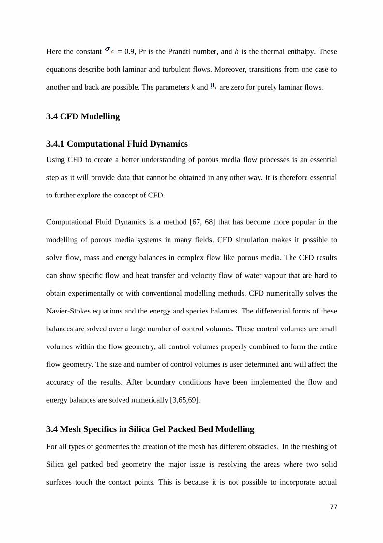
77
Here the constant = 0.9, Pr is the Prandtl number, and h is the thermal enthalpy. These
equations describe both laminar and turbulent flows. Moreover, transitions from one case to
another and back are possible. The parameters k and are zero for purely laminar flows.
3.4 CFD Modelling
3.4.1 Computational Fluid Dynamics
Using CFD to create a better understanding of porous media flow processes is an essential
step as it will provide data that cannot be obtained in any other way. It is therefore essential
to further explore the concept of CFD.
Computational Fluid Dynamics is a method [67, 68] that has become more popular in the
modelling of porous media systems in many fields. CFD simulation makes it possible to
solve flow, mass and energy balances in complex flow like porous media. The CFD results
can show specific flow and heat transfer and velocity flow of water vapour that are hard to
obtain experimentally or with conventional modelling methods. CFD numerically solves the
Navier-Stokes equations and the energy and species balances. The differential forms of these
balances are solved over a large number of control volumes. These control volumes are small
volumes within the flow geometry, all control volumes properly combined to form the entire
flow geometry. The size and number of control volumes is user determined and will affect the
accuracy of the results. After boundary conditions have been implemented the flow and
energy balances are solved numerically [3,65,69].
3.4 Mesh Specifics in Silica Gel Packed Bed Modelling
For all types of geometries the creation of the mesh has different obstacles. In the meshing of
Silica gel packed bed geometry the major issue is resolving the areas where two solid
surfaces touch the contact points. This is because it is not possible to incorporate actual
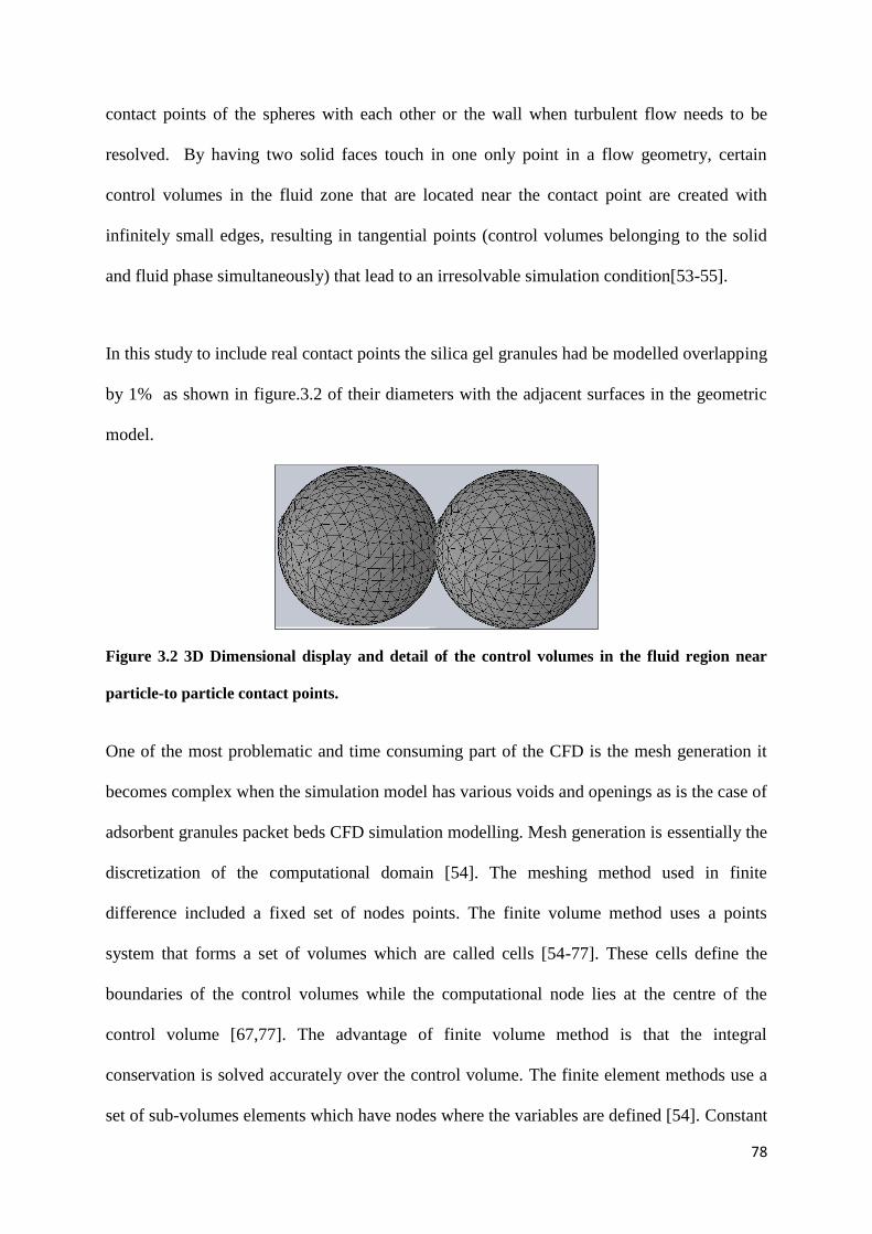
78
contact points of the spheres with each other or the wall when turbulent flow needs to be
resolved. By having two solid faces touch in one only point in a flow geometry, certain
control volumes in the fluid zone that are located near the contact point are created with
infinitely small edges, resulting in tangential points (control volumes belonging to the solid
and fluid phase simultaneously) that lead to an irresolvable simulation condition[53-55].
In this study to include real contact points the silica gel granules had be modelled overlapping
by 1% as shown in figure.3.2 of their diameters with the adjacent surfaces in the geometric
model.
Figure 3.2 3D Dimensional display and detail of the control volumes in the fluid region near
particle-to particle contact points.
One of the most problematic and time consuming part of the CFD is the mesh generation it
becomes complex when the simulation model has various voids and openings as is the case of
adsorbent granules packet beds CFD simulation modelling. Mesh generation is essentially the
discretization of the computational domain [54]. The meshing method used in finite
difference included a fixed set of nodes points. The finite volume method uses a points
system that forms a set of volumes which are called cells [54-77]. These cells define the
boundaries of the control volumes while the computational node lies at the centre of the
control volume [67,77]. The advantage of finite volume method is that the integral
conservation is solved accurately over the control volume. The finite element methods use a
set of sub-volumes elements which have nodes where the variables are defined [54]. Constant
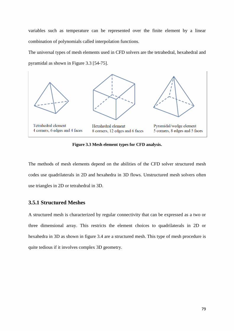
79
variables such as temperature can be represented over the finite element by a linear
combination of polynomials called interpolation functions.
The universal types of mesh elements used in CFD solvers are the tetrahedral, hexahedral and
pyramidal as shown in Figure 3.3 [54-75].
Figure 3.3 Mesh element types for CFD analysis.
The methods of mesh elements depend on the abilities of the CFD solver structured mesh
codes use quadrilaterals in 2D and hexahedra in 3D flows. Unstructured mesh solvers often
use triangles in 2D or tetrahedral in 3D.
3.5.1 Structured Meshes
A structured mesh is characterized by regular connectivity that can be expressed as a two or
three dimensional array. This restricts the element choices to quadrilaterals in 2D or
hexahedra in 3D as shown in figure 3.4 are a structured mesh. This type of mesh procedure is
quite tedious if it involves complex 3D geometry.
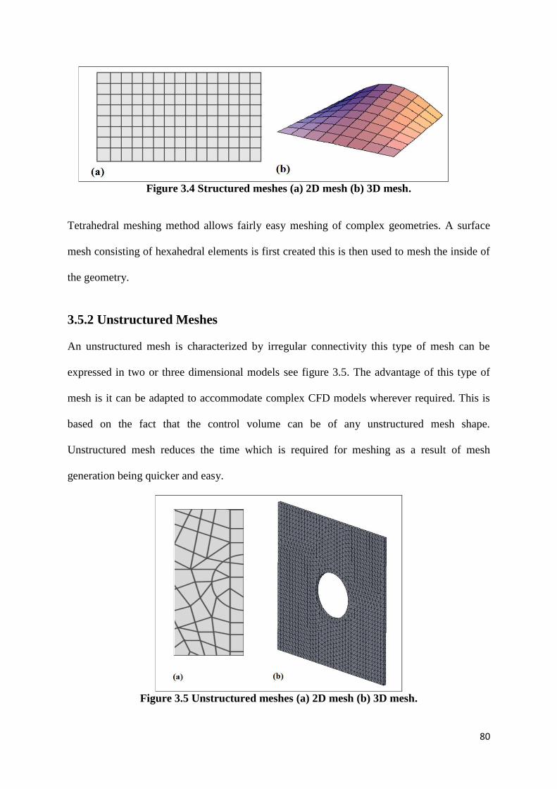
80
Figure 3.4 Structured meshes (a) 2D mesh (b) 3D mesh.
Tetrahedral meshing method allows fairly easy meshing of complex geometries. A surface
mesh consisting of hexahedral elements is first created this is then used to mesh the inside of
the geometry.
3.5.2 Unstructured Meshes
An unstructured mesh is characterized by irregular connectivity this type of mesh can be
expressed in two or three dimensional models see figure 3.5. The advantage of this type of
mesh is it can be adapted to accommodate complex CFD models wherever required. This is
based on the fact that the control volume can be of any unstructured mesh shape.
Unstructured mesh reduces the time which is required for meshing as a result of mesh
generation being quicker and easy.
Figure 3.5 Unstructured meshes (a) 2D mesh (b) 3D mesh.
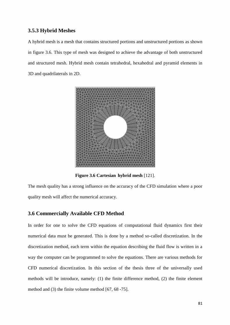
81
3.5.3 Hybrid Meshes
A hybrid mesh is a mesh that contains structured portions and unstructured portions as shown
in figure 3.6. This type of mesh was designed to achieve the advantage of both unstructured
and structured mesh. Hybrid mesh contain tetrahedral, hexahedral and pyramid elements in
3D and quadrilaterals in 2D.
Figure 3.6 Cartesian hybrid mesh [121].
The mesh quality has a strong influence on the accuracy of the CFD simulation where a poor
quality mesh will affect the numerical accuracy.
3.6 Commercially Available CFD Method
In order for one to solve the CFD equations of computational fluid dynamics first their
numerical data must be generated. This is done by a method so-called discretization. In the
discretization method, each term within the equation describing the fluid flow is written in a
way the computer can be programmed to solve the equations. There are various methods for
CFD numerical discretization. In this section of the thesis three of the universally used
methods will be introduce, namely: (1) the finite difference method, (2) the finite element
method and (3) the finite volume method [67, 68 -75].
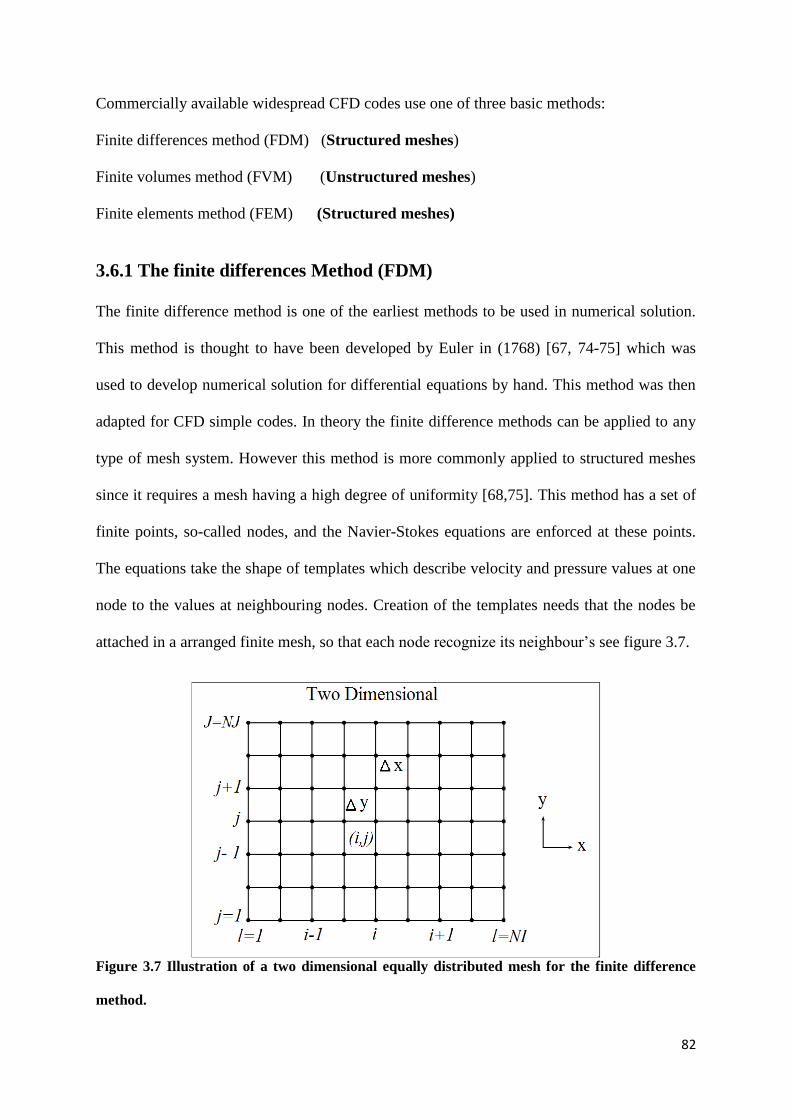
82
Commercially available widespread CFD codes use one of three basic methods:
Finite differences method (FDM) (Structured meshes)
Finite volumes method (FVM) (Unstructured meshes)
Finite elements method (FEM) (Structured meshes)
3.6.1 The finite differences Method (FDM)
The finite difference method is one of the earliest methods to be used in numerical solution.
This method is thought to have been developed by Euler in (1768) [67, 74-75] which was
used to develop numerical solution for differential equations by hand. This method was then
adapted for CFD simple codes. In theory the finite difference methods can be applied to any
type of mesh system. However this method is more commonly applied to structured meshes
since it requires a mesh having a high degree of uniformity [68,75]. This method has a set of
finite points, so-called nodes, and the Navier-Stokes equations are enforced at these points.
The equations take the shape of templates which describe velocity and pressure values at one
node to the values at neighbouring nodes. Creation of the templates needs that the nodes be
attached in a arranged finite mesh, so that each node recognize its neighbour’s see figure 3.7.
Figure 3.7 Illustration of a two dimensional equally distributed mesh for the finite difference
method.
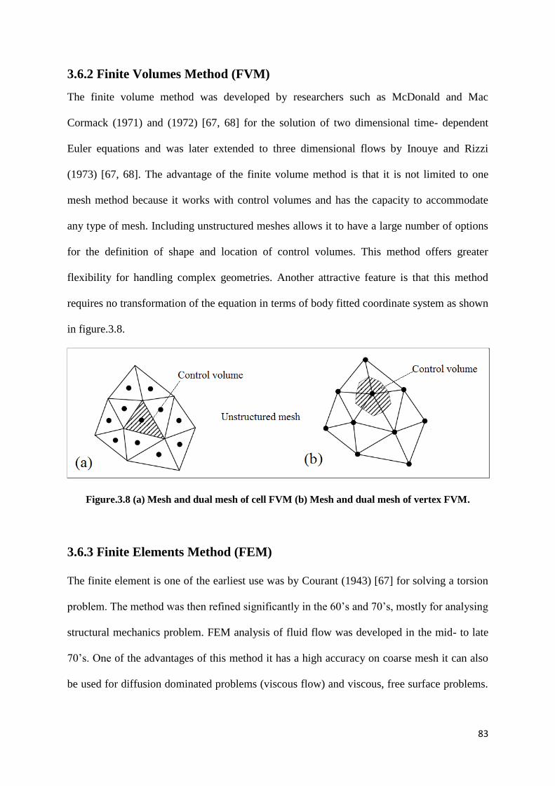
83
3.6.2 Finite Volumes Method (FVM)
The finite volume method was developed by researchers such as McDonald and Mac
Cormack (1971) and (1972) [67, 68] for the solution of two dimensional time- dependent
Euler equations and was later extended to three dimensional flows by Inouye and Rizzi
(1973) [67, 68]. The advantage of the finite volume method is that it is not limited to one
mesh method because it works with control volumes and has the capacity to accommodate
any type of mesh. Including unstructured meshes allows it to have a large number of options
for the definition of shape and location of control volumes. This method offers greater
flexibility for handling complex geometries. Another attractive feature is that this method
requires no transformation of the equation in terms of body fitted coordinate system as shown
in figure.3.8.
Figure.3.8 (a) Mesh and dual mesh of cell FVM (b) Mesh and dual mesh of vertex FVM.
3.6.3 Finite Elements Method (FEM)
The finite element is one of the earliest use was by Courant (1943) [67] for solving a torsion
problem. The method was then refined significantly in the 60’s and 70’s, mostly for analysing
structural mechanics problem. FEM analysis of fluid flow was developed in the mid- to late
70’s. One of the advantages of this method it has a high accuracy on coarse mesh it can also
be used for diffusion dominated problems (viscous flow) and viscous, free surface problems.
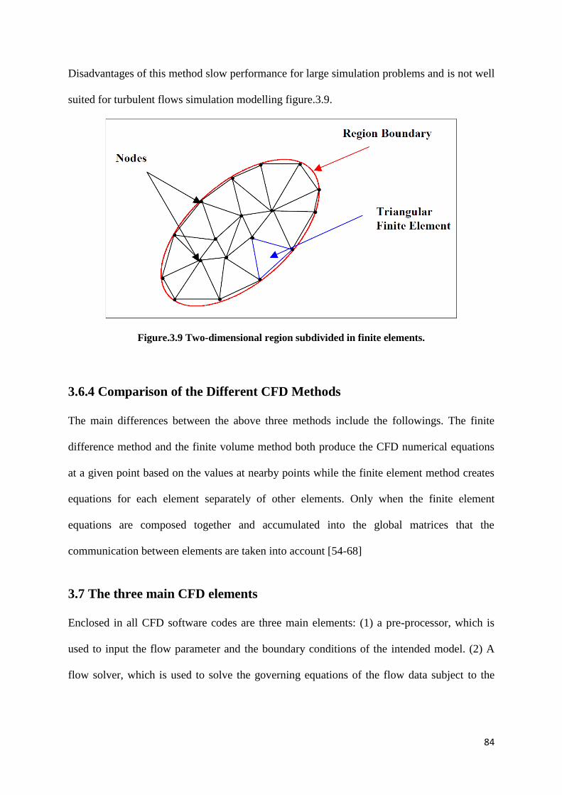
84
Disadvantages of this method slow performance for large simulation problems and is not well
suited for turbulent flows simulation modelling figure.3.9.
Figure.3.9 Two-dimensional region subdivided in finite elements.
3.6.4 Comparison of the Different CFD Methods
The main differences between the above three methods include the followings. The finite
difference method and the finite volume method both produce the CFD numerical equations
at a given point based on the values at nearby points while the finite element method creates
equations for each element separately of other elements. Only when the finite element
equations are composed together and accumulated into the global matrices that the
communication between elements are taken into account [54-68]
3.7 The three main CFD elements
Enclosed in all CFD software codes are three main elements: (1) a pre-processor, which is
used to input the flow parameter and the boundary conditions of the intended model. (2) A
flow solver, which is used to solve the governing equations of the flow data subject to the
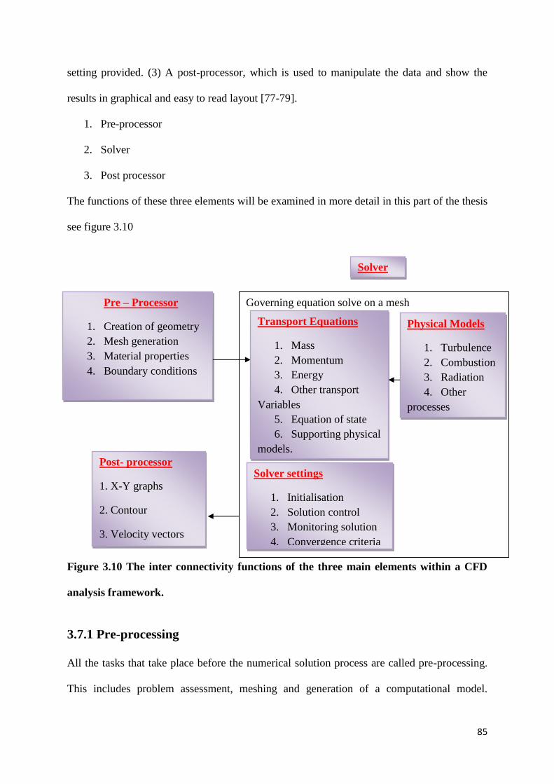
85
setting provided. (3) A post-processor, which is used to manipulate the data and show the
results in graphical and easy to read layout [77-79].
1. Pre-processor
2. Solver
3. Post processor
The functions of these three elements will be examined in more detail in this part of the thesis
see figure 3.10
Figure 3.10 The inter connectivity functions of the three main elements within a CFD
analysis framework.
3.7.1 Pre-processing
All the tasks that take place before the numerical solution process are called pre-processing.
This includes problem assessment, meshing and generation of a computational model.
Pre – Processor
1. Creation of geometry
2. Mesh generation
3. Material properties
4. Boundary conditions
Solver
Governing equation solve on a mesh
Transport Equations
1. Mass
2. Momentum
3. Energy
4. Other transport
Variables
5. Equation of state
6. Supporting physical
models.
Physical Models
1. Turbulence
2. Combustion
3. Radiation
4. Other
processes
Solver settings
1. Initialisation
2. Solution control
3. Monitoring solution
4. Convergence criteria
Post- processor
1. X-Y graphs
2. Contour
3. Velocity vectors
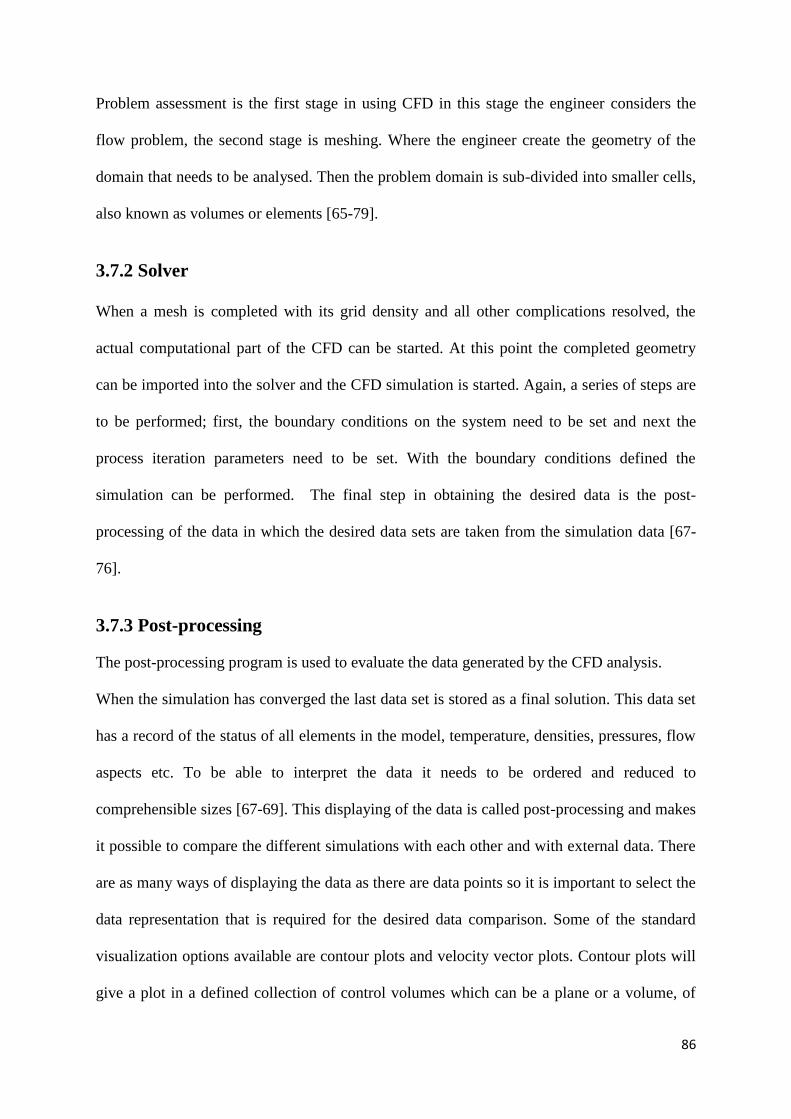
86
Problem assessment is the first stage in using CFD in this stage the engineer considers the
flow problem, the second stage is meshing. Where the engineer create the geometry of the
domain that needs to be analysed. Then the problem domain is sub-divided into smaller cells,
also known as volumes or elements [65-79].
3.7.2 Solver
When a mesh is completed with its grid density and all other complications resolved, the
actual computational part of the CFD can be started. At this point the completed geometry
can be imported into the solver and the CFD simulation is started. Again, a series of steps are
to be performed; first, the boundary conditions on the system need to be set and next the
process iteration parameters need to be set. With the boundary conditions defined the
simulation can be performed. The final step in obtaining the desired data is the post-
processing of the data in which the desired data sets are taken from the simulation data [67-
76].
3.7.3 Post-processing
The post-processing program is used to evaluate the data generated by the CFD analysis.
When the simulation has converged the last data set is stored as a final solution. This data set
has a record of the status of all elements in the model, temperature, densities, pressures, flow
aspects etc. To be able to interpret the data it needs to be ordered and reduced to
comprehensible sizes [67-69]. This displaying of the data is called post-processing and makes
it possible to compare the different simulations with each other and with external data. There
are as many ways of displaying the data as there are data points so it is important to select the
data representation that is required for the desired data comparison. Some of the standard
visualization options available are contour plots and velocity vector plots. Contour plots will
give a plot in a defined collection of control volumes which can be a plane or a volume, of
87
contours of another variable. For example a plane can be defined as a constant x-coordinate
plane (y-z plane); we can then make a contour plot showing temperature contours in this
plane.
In the same plane a velocity contour plot can be made showing absolute velocities of the fluid
in the defined plane [60-77]. Other variables that can be used for contour plots are magnitude
of velocity components turbulence components and local pressure. Velocity vector plots can
be made to get an insight into the flow patterns in the overall geometry or detailed at specific
locations. The density and magnification of the velocity vectors in the specified field can be
manually changed to get a most optimal picture [60-73].
The field density has a maximum limitation, the amount of elements in the model. Besides
these qualitative data export methods it is also possible to export the numerical data in many
different forms [3,73]. Direct export of selected data sets is facilitated for a number of
external applications. It is also possible to export data in Parasolid format for further
manipulation. Another method for exporting the numerical data is the two-dimensional plot
function in which two data sets can be plotted against each other [54-80]. This function is
useful when, for example, radial velocity or temperature profiles need to be compared. From
different simulations, identical plots can be created and a direct comparison of the numerical
data is possible [75-80].
3.8 CAD Geometry Design
In this phase of the model design the major topological entities are defined. The outer wall to
the model is established as well as the internal structure, solid particles and fluid regions.
Several entities, such as cylinders or spheres, are ready made parts that can be added to the
geometry. Before exporting the fundamental geometry it is important all curves are defined as
so-called B-Spline curves, these are mathematical descriptions of the specific curves. This
88
conversion is necessary to be able to have the surface mesh form to the exact contours of the
created geometry.
3.9 Imposing Boundary Conditions Inlet and Outlet
The boundary conditions take into account numerous elements that affect the behaviour of
fluids and help to visualize them through 3D simulation. Some of these elements consist of
mass transfer, heat flow, and changes in gas to liquid and liquid to gas phases. Boundary
conditions contribute to the understanding of what results are possible at the inlet and outlet
of a model [54].
External Faces
1. Flow inlet and exit boundaries: pressure inlet, velocity inlet pressure outlet, outflow.
2. Wall repeating and boundaries: wall symmetry
3. Internal zones: fluid
4. Internal face boundaries porous media silica gel interior
Figure.3.11 Establishing by setting the iteration parameters.
3.10 Validating CFD against Experimental Data
This study has used CFD for detailed modelling of heat and mass transfer in an adsorption
system adsorbent bed. One of the major questions in CFD simulation modelling is whether it
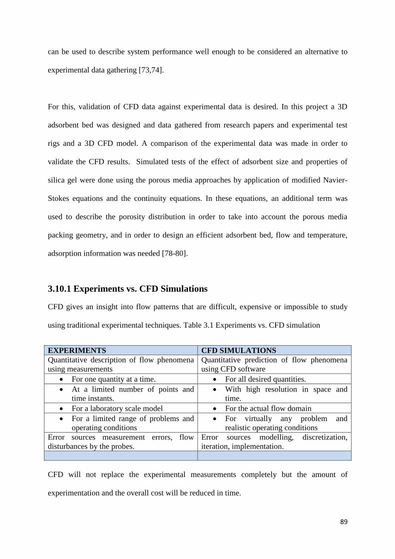
89
can be used to describe system performance well enough to be considered an alternative to
experimental data gathering [73,74].
For this, validation of CFD data against experimental data is desired. In this project a 3D
adsorbent bed was designed and data gathered from research papers and experimental test
rigs and a 3D CFD model. A comparison of the experimental data was made in order to
validate the CFD results. Simulated tests of the effect of adsorbent size and properties of
silica gel were done using the porous media approaches by application of modified Navier-
Stokes equations and the continuity equations. In these equations, an additional term was
used to describe the porosity distribution in order to take into account the porous media
packing geometry, and in order to design an efficient adsorbent bed, flow and temperature,
adsorption information was needed [78-80].
3.10.1 Experiments vs. CFD Simulations
CFD gives an insight into flow patterns that are difficult, expensive or impossible to study
using traditional experimental techniques. Table 3.1 Experiments vs. CFD simulation
EXPERIMENTS CFD SIMULATIONS
Quantitative description of flow phenomena
using measurements
Quantitative prediction of flow phenomena
using CFD software
For one quantity at a time. For all desired quantities.
At a limited number of points and
time instants.
With high resolution in space and
time.
For a laboratory scale model For the actual flow domain
For a limited range of problems and
operating conditions
For virtually any problem and
realistic operating conditions
Error sources measurement errors, flow
disturbances by the probes.
Error sources modelling, discretization,
iteration, implementation.
CFD will not replace the experimental measurements completely but the amount of
experimentation and the overall cost will be reduced in time.
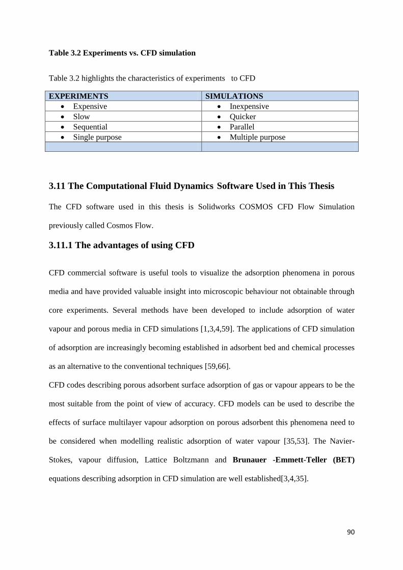
90
Table 3.2 Experiments vs. CFD simulation
Table 3.2 highlights the characteristics of experiments to CFD
EXPERIMENTS SIMULATIONS
Expensive Inexpensive
Slow Quicker
Sequential Parallel
Single purpose Multiple purpose
3.11 The Computational Fluid Dynamics Software Used in This Thesis
The CFD software used in this thesis is Solidworks COSMOS CFD Flow Simulation
previously called Cosmos Flow.
3.11.1 The advantages of using CFD
CFD commercial software is useful tools to visualize the adsorption phenomena in porous
media and have provided valuable insight into microscopic behaviour not obtainable through
core experiments. Several methods have been developed to include adsorption of water
vapour and porous media in CFD simulations [1,3,4,59]. The applications of CFD simulation
of adsorption are increasingly becoming established in adsorbent bed and chemical processes
as an alternative to the conventional techniques [59,66].
CFD codes describing porous adsorbent surface adsorption of gas or vapour appears to be the
most suitable from the point of view of accuracy. CFD models can be used to describe the
effects of surface multilayer vapour adsorption on porous adsorbent this phenomena need to
be considered when modelling realistic adsorption of water vapour [35,53]. The Navier-
Stokes, vapour diffusion, Lattice Boltzmann and Brunauer -Emmett-Teller (BET)
equations describing adsorption in CFD simulation are well established[3,4,35].
91
3.11.3 The limitation of CFD modelling when dealing with chemical
adsorption of vapour
CFD commercial software has the capability to model physical surface adsorption of vapour
transport within porous adsorbent regions [6,7]. However, this capability is somewhat limited
when extended to chemical adsorption phenomena of vapour in porous adsorbent regions.
This restricts the modelling of adsorption to mainly physical surface modelling of the
adsorption of vapour or gasses [59,72].
This is not a problem when studying adsorption cooling systems because the adsorption
taking place in the adsorption cooling system is of a physical surface adsorption phenomenon
only. However, this can be more difficult when attempting the simulation of a chemical
adsorption system. There are hybrid CFD software packages specifically developed for
modelling complex chemical adsorption such as CHEMKIN [131], CANTERA [132],
DETCHEM [133], which also offer CFD codes for special reactor configurations such as
channel flows and monolithic reactors. These kinetic packages also have a variety of user
written subroutines for modelling complex reaction a variety of multi-purpose and
specialized CFD codes.
Another limitation of CFD adsorption simulation of vapour is the computer power needed to
correctly model adsorption, which limits CFD simulation to only to small section of an
adsorbent bed.
3.12 The Different Types of CFD Simulation Software Package
When selecting a CFD simulation software package you are faced with a large selection of
options. There is a vast range of computational fluid dynamic systems available, from
general-purpose CFD software through to very specific application software. There are some
CFD programs that will provide results for pipe systems only whilst others will work only
92
with 2D CFD Simulation methods. Some general purpose CFD software can be versatile in
different area of CFD modelling but not specialist.
There are three types of CFD simulation areas:
3.12.1 Commercial off the Shelf CFD Simulation Software Packages
These are CFD packages developed and supported by commercial organizations the leading
general purpose products are:
• COSMOS FLOW SIMULATION
• COMSOL MULTIPHYSICS
• STAR-CD
• FLUENT
• CFX
Each software program has advantages and disadvantages.
3.12.2 Custom-built CFD Simulation Specialist Software
The advantages of custom built CFD simulation software over general-purpose CFD
simulation software both industrial and academic develop CFD programmes in-house for
their own user base. Large industrial establishments, for instance, have a tendency to rely
greatly on custom-built CFD system because they need high accuracy results.
3.12.3 CFD Freeware Software
Open FOAM
OpenFOAM is a universal CFD code written in C++ the package comprises of modules for a
wide range of CFD simulation procedures. OpenFOAM was written by Henry Weller and
others at Imperial College. This is just one of the several CFD freeware software that can be
download from the internet.
93
3.13 Conclusion
At presently CFD simulation method is largely used in engineering application to provide
data that is complementary to experimental and theoretical results. This simulation method is
becoming more common in academic establishments and government research laboratories.
One of the reasons for this can be partially accredited to the rapid evolution of CFD methods
especially through the availability of multipurpose commercial CFD computer programs.
Also with the decreasing costs of computer hardware and fast computing speed engineers are
increasingly relying on this reliable simulation tool. In conclusion to this chapter one can
continue to believe as the future unfolds CFD simulation and its modelling methods will
continue to remain at the forefront of increasing research and development as long as the vast
majority of complex fluid flow solution remains unanswered.
94
CHAPTER 4
COMPUTATIONAL FLUID DYNAMICS MODELLING AND
EXPERIMENTAL STUDY ON A SILICA GEL TYPE B
Abstract
The last chapter has provided reviews of basic underlying principles of CFD this will serve as
an essential knowledge for this chapter. The application of computational fluid dynamics
(CFDs) in the area of porous media and adsorption cooling system is becoming more
practical due to the significant improvement in computer power. The results from previous
studies have shown that CFD can be useful tool for predicting the water vapour flow pattern,
temperature, heat transfer and flow velocity and adsorption rate. This chapter investigates the
effect of silica gel granular size on the water adsorption rate using computational fluid
dynamics and gravimetric experimental (DVS) method.
4.1 Introduction
The adsorption properties of silica gel have been studied for many years as silica gel is used
in many industries including adsorption cooling systems. Past research have shown
experimentally that the adsorption rate of silica gel granules depend on their size. The
purpose of this work was to study the effect of granule size on the adsorption properties of
silica gel by using CFD and comparing the simulation results to those obtained
experimentally. (CFD) Computational Fluid Dynamics is a field that has developed over the
years because of the new development of computers and CFD simulation. CFD is also used a
simulation tool in refrigeration and air conditioning industry. In this chapter CFD simulation
have been used for modelling of heat and mass transfer in a adsorption tube with silica. One
of the questions in CFD modelling is can this type of technology be used as an alternative to
experimental data gathering. For this hypothesis a confirmation of CFD data against
95
experimental data is desired. In this chapter a 3D silica gel and tube structured model have
been developed for this purpose. Data will be gathered from experimental study of identical
CFD model. This data will be compared to experimental and CFD results. The effects of
silica gel size and properties have been studied using the porous media approaches by
application of modified Navier-Stokes equations and the continuity equation. In this set of
equations, an additional term is used describing the porosity distribution in order to take into
account the porous media packing geometry.
To design an efficient adsorbent bed, flow and temperature information is essential. Studies
of fluid dynamics and heat transfer in adsorbent beds date back to the early twentieth century
[6]. The early investigation of flow in porous media packed beds provided mainly such bulk
information as pressure drop correlations. For example, Ergun [82] Andersson suggested a
pressure loss equation, in which parameters like porous media particle diameter and fluid
physical properties were used to correlate the pressure drop. Similar correlations were
proposed by Molerus [63].
These three empirical correlations rather well predict pressure loss for flow in adsorbent beds
but provide nothing more about local flow fields our adsorption/desorption on porous media.
On the other hand, of the many investigations of heat transfer in adsorbent beds in the last
several decades, effective parameter methods were applied to predict temperature distribution
[3,83].
CFD (computational fluid dynamics) provides an innovative approach to model and
analysing the local flow and the effect of silica gel size on adsorption performance of a
packed bed. Numerical simulation of porous media local flow and heat transfer based on the
CFD technique has increasingly been reported in recent years in fields of packed bed flow
and heat transfer modelling [84]. In this work, a finite volume formulation based on the
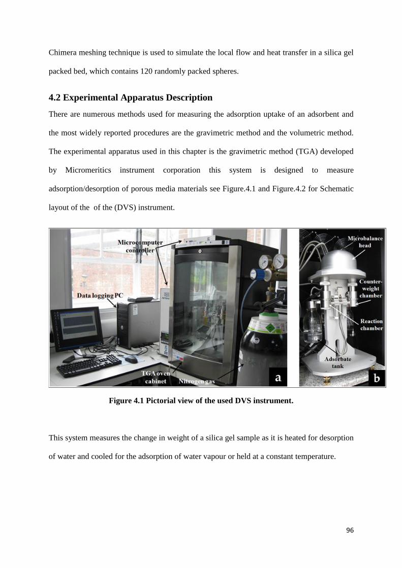
96
Chimera meshing technique is used to simulate the local flow and heat transfer in a silica gel
packed bed, which contains 120 randomly packed spheres.
4.2 Experimental Apparatus Description
There are numerous methods used for measuring the adsorption uptake of an adsorbent and
the most widely reported procedures are the gravimetric method and the volumetric method.
The experimental apparatus used in this chapter is the gravimetric method (TGA) developed
by Micromeritics instrument corporation this system is designed to measure
adsorption/desorption of porous media materials see Figure.4.1 and Figure.4.2 for Schematic
layout of the of the (DVS) instrument.
Figure 4.1 Pictorial view of the used DVS instrument.
This system measures the change in weight of a silica gel sample as it is heated for desorption
of water and cooled for the adsorption of water vapour or held at a constant temperature.
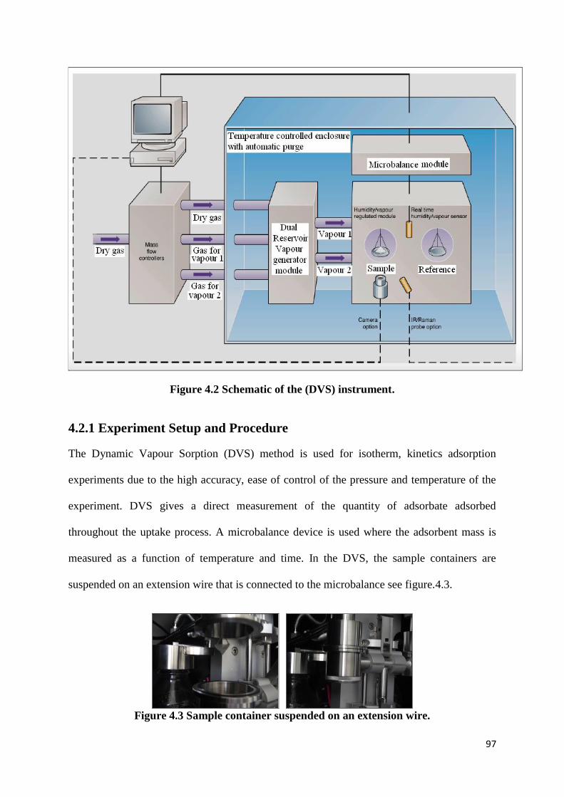
97
Figure 4.2 Schematic of the (DVS) instrument.
4.2.1 Experiment Setup and Procedure
The Dynamic Vapour Sorption (DVS) method is used for isotherm, kinetics adsorption
experiments due to the high accuracy, ease of control of the pressure and temperature of the
experiment. DVS gives a direct measurement of the quantity of adsorbate adsorbed
throughout the uptake process. A microbalance device is used where the adsorbent mass is
measured as a function of temperature and time. In the DVS, the sample containers are
suspended on an extension wire that is connected to the microbalance see figure.4.3.
Figure 4.3 Sample container suspended on an extension wire.
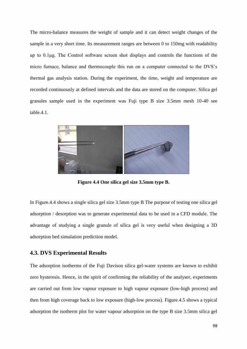
98
The micro-balance measures the weight of sample and it can detect weight changes of the
sample in a very short time. Its measurement ranges are between 0 to 150mg with readability
up to 0.1μg. The Control software screen shot displays and controls the functions of the
micro furnace, balance and thermocouple this run on a computer connected to the DVS’s
thermal gas analysis station. During the experiment, the time, weight and temperature are
recorded continuously at defined intervals and the data are stored on the computer. Silica gel
granules sample used in the experiment was Fuji type B size 3.5mm mesh 10-40 see
table.4.1.
Figure 4.4 One silica gel size 3.5mm type B.
In Figure.4.4 shows a single silica gel size 3.5mm type B The purpose of testing one silica gel
adsorption / desorption was to generate experimental data to be used in a CFD module. The
advantage of studying a single granule of silica gel is very useful when designing a 3D
adsorption bed simulation prediction model.
4.3. DVS Experimental Results
The adsorption isotherms of the Fuji Davison silica gel-water systems are known to exhibit
zero hysteresis. Hence, in the spirit of confirming the reliability of the analyser, experiments
are carried out from low vapour exposure to high vapour exposure (low-high process) and
then from high coverage back to low exposure (high-low process). Figure.4.5 shows a typical
adsorption the isotherm plot for water vapour adsorption on the type B size 3.5mm silica gel
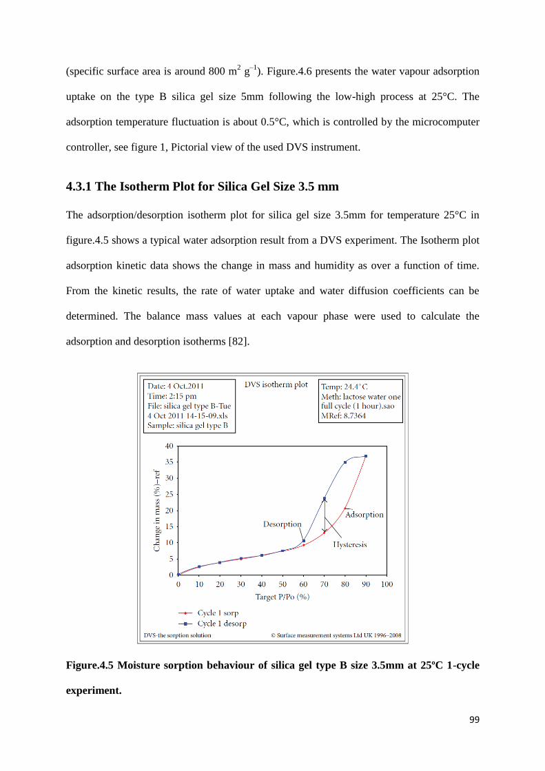
99
(specific surface area is around 800 m2 g
–1). Figure.4.6 presents the water vapour adsorption
uptake on the type B silica gel size 5mm following the low-high process at 25°C. The
adsorption temperature fluctuation is about 0.5°C, which is controlled by the microcomputer
controller, see figure 1, Pictorial view of the used DVS instrument.
4.3.1 The Isotherm Plot for Silica Gel Size 3.5 mm
The adsorption/desorption isotherm plot for silica gel size 3.5mm for temperature 25°C in
figure.4.5 shows a typical water adsorption result from a DVS experiment. The Isotherm plot
adsorption kinetic data shows the change in mass and humidity as over a function of time.
From the kinetic results, the rate of water uptake and water diffusion coefficients can be
determined. The balance mass values at each vapour phase were used to calculate the
adsorption and desorption isotherms [82].
Figure.4.5 Moisture sorption behaviour of silica gel type B size 3.5mm at 25ºC 1-cycle
experiment.
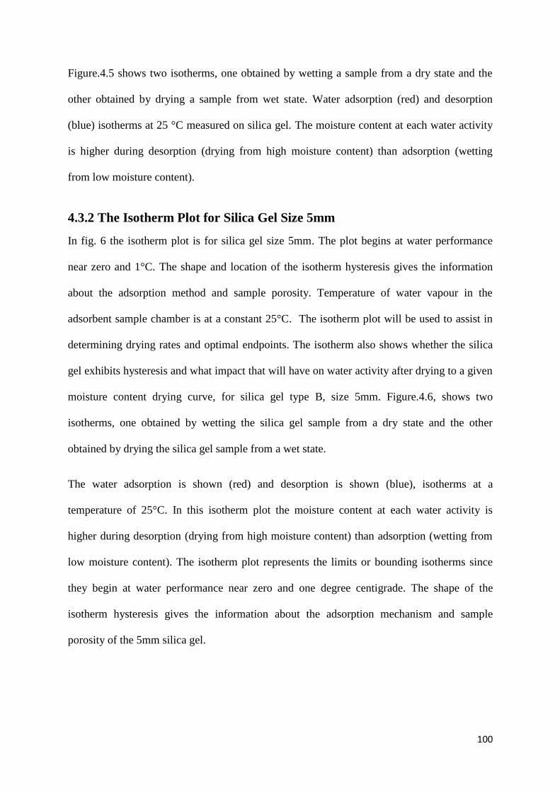
100
Figure.4.5 shows two isotherms, one obtained by wetting a sample from a dry state and the
other obtained by drying a sample from wet state. Water adsorption (red) and desorption
(blue) isotherms at 25 °C measured on silica gel. The moisture content at each water activity
is higher during desorption (drying from high moisture content) than adsorption (wetting
from low moisture content).
4.3.2 The Isotherm Plot for Silica Gel Size 5mm
In fig. 6 the isotherm plot is for silica gel size 5mm. The plot begins at water performance
near zero and 1°C. The shape and location of the isotherm hysteresis gives the information
about the adsorption method and sample porosity. Temperature of water vapour in the
adsorbent sample chamber is at a constant 25°C. The isotherm plot will be used to assist in
determining drying rates and optimal endpoints. The isotherm also shows whether the silica
gel exhibits hysteresis and what impact that will have on water activity after drying to a given
moisture content drying curve, for silica gel type B, size 5mm. Figure.4.6, shows two
isotherms, one obtained by wetting the silica gel sample from a dry state and the other
obtained by drying the silica gel sample from a wet state.
The water adsorption is shown (red) and desorption is shown (blue), isotherms at a
temperature of 25°C. In this isotherm plot the moisture content at each water activity is
higher during desorption (drying from high moisture content) than adsorption (wetting from
low moisture content). The isotherm plot represents the limits or bounding isotherms since
they begin at water performance near zero and one degree centigrade. The shape of the
isotherm hysteresis gives the information about the adsorption mechanism and sample
porosity of the 5mm silica gel.
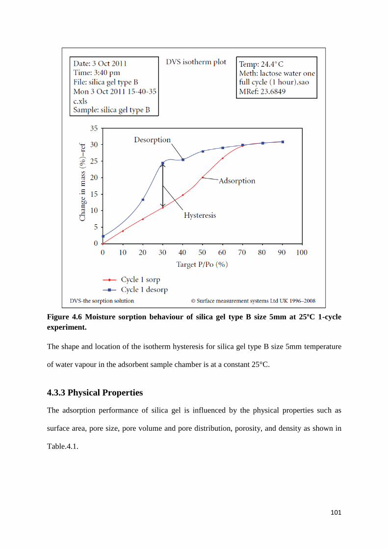
101
Figure 4.6 Moisture sorption behaviour of silica gel type B size 5mm at 25ºC 1-cycle
experiment.
The shape and location of the isotherm hysteresis for silica gel type B size 5mm temperature
of water vapour in the adsorbent sample chamber is at a constant 25°C.
4.3.3 Physical Properties
The adsorption performance of silica gel is influenced by the physical properties such as
surface area, pore size, pore volume and pore distribution, porosity, and density as shown in
Table.4.1.
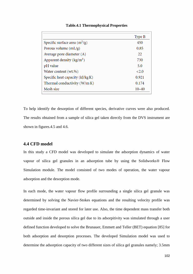
102
Table.4.1 Thermophysical Properties
To help identify the desorption of different species, derivative curves were also produced.
The results obtained from a sample of silica gel taken directly from the DVS instrument are
shown in figures.4.5 and 4.6.
4.4 CFD model
In this study a CFD model was developed to simulate the adsorption dynamics of water
vapour of silica gel granules in an adsorption tube by using the Solidworks® Flow
Simulation module. The model consisted of two modes of operation, the water vapour
adsorption and the desorption mode.
In each mode, the water vapour flow profile surrounding a single silica gel granule was
determined by solving the Navier-Stokes equations and the resulting velocity profile was
regarded time-invariant and stored for later use. Also, the time dependent mass transfer both
outside and inside the porous silica gel due to its adsorpitivity was simulated through a user
defined function developed to solve the Brunauer, Emmett and Teller (BET) equation [85] for
both adsorption and desorption processes. The developed Simulation model was used to
determine the adsorption capacity of two different sizes of silica gel granules namely; 3.5mm
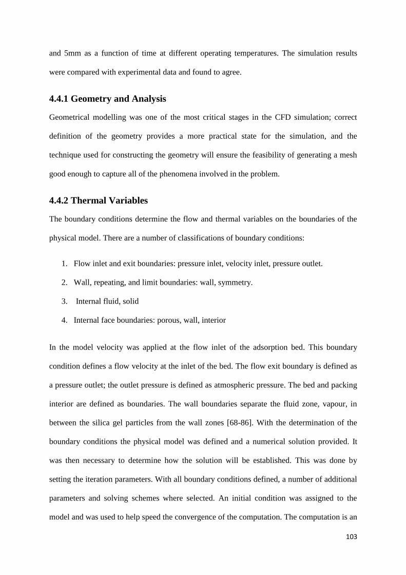
103
and 5mm as a function of time at different operating temperatures. The simulation results
were compared with experimental data and found to agree.
4.4.1 Geometry and Analysis
Geometrical modelling was one of the most critical stages in the CFD simulation; correct
definition of the geometry provides a more practical state for the simulation, and the
technique used for constructing the geometry will ensure the feasibility of generating a mesh
good enough to capture all of the phenomena involved in the problem.
4.4.2 Thermal Variables
The boundary conditions determine the flow and thermal variables on the boundaries of the
physical model. There are a number of classifications of boundary conditions:
1. Flow inlet and exit boundaries: pressure inlet, velocity inlet, pressure outlet.
2. Wall, repeating, and limit boundaries: wall, symmetry.
3. Internal fluid, solid
4. Internal face boundaries: porous, wall, interior
In the model velocity was applied at the flow inlet of the adsorption bed. This boundary
condition defines a flow velocity at the inlet of the bed. The flow exit boundary is defined as
a pressure outlet; the outlet pressure is defined as atmospheric pressure. The bed and packing
interior are defined as boundaries. The wall boundaries separate the fluid zone, vapour, in
between the silica gel particles from the wall zones [68-86]. With the determination of the
boundary conditions the physical model was defined and a numerical solution provided. It
was then necessary to determine how the solution will be established. This was done by
setting the iteration parameters. With all boundary conditions defined, a number of additional
parameters and solving schemes where selected. An initial condition was assigned to the
model and was used to help speed the convergence of the computation. The computation is an
104
iterative process that solves the governing equations for flow and energy in each simulated
cell.
4.4.3 Modelling of Vapour Flow in a Single Silica Gel Particle
The diffusion equation in the silica gel particle is as a first introduction to CFD. A simple
model was created; the model represented one silica granule in a tube as shown in
(Figure.4.7) the flow inlet and flow outlet.
Figure 4.7 One silica gel in a tube geometry used for validation of CFD against
experimental work.
4.4.4 Porous Media Simulations
A porous material had to be defined for the adsorbent used in the simulation. This data was
taken from the experiment Type B size 3.5mm data was created with a density of 730 kg/m3,
and for type B size 5mm a density of 730 kg/m3 and a heat capacity of 0.921 J/kg K and a
thermal conductivity of 0.174 W/ m K (See Table.4 .1).
4.4.5 CFD Porous Medium Methodology
For the porous medium approach the CFD model has a mass of cells representing the fluid
inlet. This is followed by the porous medium cells, which are used to model fluid flow
through porous medium. Full flow field predictions are possible with the porous medium
approach because the resistance of the porous medium to flow is described by the expression:
105
(1)
Where the permeability coefficient values α and β are assigned temperature dependent values
that describe the behaviour of a porous medium. High values of α and β preclude flow at
right angles to the porous medium. Upstream and downstream of the water vapour flow field
is solved using the usual Reynolds averaged Navier-Stokes methodology.
Table.4.2 Thermophysical Properties Used in CFD simulation
4.4.6 Model Mesh
One of the most important parts of this CFD simulation was the module mesh creation. The
mesh which establishes the accuracy of the simulation has to be chosen with enough detail to
describe the simulation processes accurately and with a degree of coarseness that enables
solution within an acceptable amount of time. When an optimal density has been found
refining this will increase the model size without displaying more flow detail. When it is
coarsened the mesh will obscure, possibly essential part of the flow detail. The mesh
determines a large part of creating an acceptable simulation.
106
4.4.7 The CFD Mesh Density
For this study we focused mainly on maintaining a 3D simulation that described the physical
model accurately and was able to handle the flow specifics of the silica gel geometry. The
mesh densities were varied to establish the optimal mesh density, describing the flow
characteristics and limiting the calculation times. The initial mesh was specified in the
following stages:
Specifying an initial mesh, so all the following specifications consist in changing the default
values of its parameters.
1. Specifying a basic mesh consisting of nearly uniform cells.
2. Refinement of the basic mesh to capture the relatively small silica gel porous features,
to resolve the small porous features in contact with fluid.
3. Refinement of the basic mesh to resolve the solid/fluid interface (as well as
porous/ solid, fluid/ porous interfaces.
4. Specifying other initial meshes in local regions (solid and/or fluid) to better resolve
the model specific geometry and/or flow (and/or heat transfer in solids) peculiarities
in these regions.
4.4.8 Simulation Data
When the simulation has converged the last data set is stored as a final solution. This data set
has a record of the status of all elements in the model, temperature, densities, pressures, flow
aspects etc. To be able to interpret the data it needs to be ordered and reduced to
comprehensible sizes. [82] This displaying of the data is called post-processing and makes it
possible to compare the different simulations with each other and with external data. There
were as many ways of displaying the data as there were data points so it was important to
select the data representation that was required for the desired data comparison. Some of the
107
standard options available are contour plots and velocity vector plots. Contour plots will give
a plot in the defined data point collection; this can be a plane or a volume, of contours of
another variable.
For example a plane can be defined as a constant x coordinate plane (y-z plane) we can then
make a contour plot showing temperature contours in this plane. In the same plane a velocity
contour plot can be made showing absolute velocities of the fluid in the defined plane. Other
variables that can be used for contour plots are magnitude of velocity components, turbulence
components, pressure etc. Velocity vector plots can be made to get an insight into the flow
patterns in the overall geometry or detailed at specific locations [85,89-90].
4.4.9 Fluid Flow Fundamentals
For iteration, CFD solvers use generalized fluid flow and energy balances based on the
Navier Stokes equations. The balances are generalized so the user can influence which
elements are added in the balance and which are not. The number of balances to be solved is
also user defined; it can be advantage not solve all balances initially. The generalized
balances that are used by the Flow simulation commercial CFD package are the Navier
Stokes equations for conservation of mass, momentum and energy in the flow geometry of
concern, together with additional sets of equations reflecting the problem needed to be solved
[82,83,90].
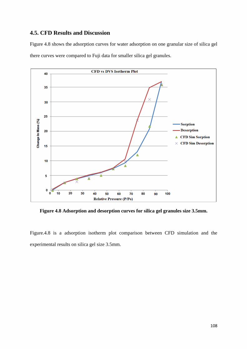
108
4.5. CFD Results and Discussion
Figure 4.8 shows the adsorption curves for water adsorption on one granular size of silica gel
there curves were compared to Fuji data for smaller silica gel granules.
Figure 4.8 Adsorption and desorption curves for silica gel granules size 3.5mm.
Figure.4.8 is a adsorption isotherm plot comparison between CFD simulation and the
experimental results on silica gel size 3.5mm.
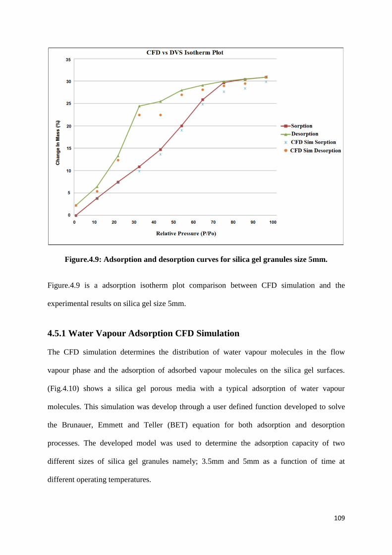
109
Figure.4.9: Adsorption and desorption curves for silica gel granules size 5mm.
Figure.4.9 is a adsorption isotherm plot comparison between CFD simulation and the
experimental results on silica gel size 5mm.
4.5.1 Water Vapour Adsorption CFD Simulation
The CFD simulation determines the distribution of water vapour molecules in the flow
vapour phase and the adsorption of adsorbed vapour molecules on the silica gel surfaces.
(Fig.4.10) shows a silica gel porous media with a typical adsorption of water vapour
molecules. This simulation was develop through a user defined function developed to solve
the Brunauer, Emmett and Teller (BET) equation for both adsorption and desorption
processes. The developed model was used to determine the adsorption capacity of two
different sizes of silica gel granules namely; 3.5mm and 5mm as a function of time at
different operating temperatures.
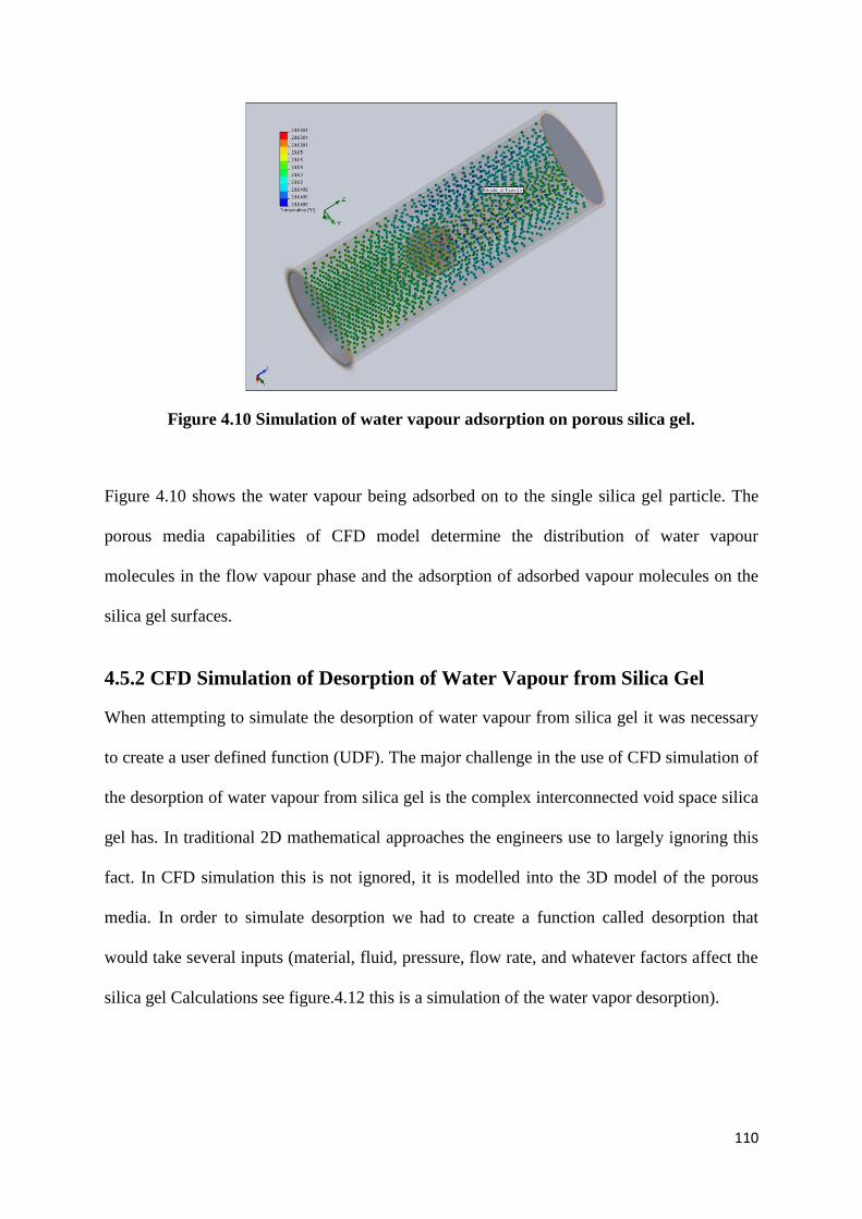
110
Figure 4.10 Simulation of water vapour adsorption on porous silica gel.
Figure 4.10 shows the water vapour being adsorbed on to the single silica gel particle. The
porous media capabilities of CFD model determine the distribution of water vapour
molecules in the flow vapour phase and the adsorption of adsorbed vapour molecules on the
silica gel surfaces.
4.5.2 CFD Simulation of Desorption of Water Vapour from Silica Gel
When attempting to simulate the desorption of water vapour from silica gel it was necessary
to create a user defined function (UDF). The major challenge in the use of CFD simulation of
the desorption of water vapour from silica gel is the complex interconnected void space silica
gel has. In traditional 2D mathematical approaches the engineers use to largely ignoring this
fact. In CFD simulation this is not ignored, it is modelled into the 3D model of the porous
media. In order to simulate desorption we had to create a function called desorption that
would take several inputs (material, fluid, pressure, flow rate, and whatever factors affect the
silica gel Calculations see figure.4.12 this is a simulation of the water vapor desorption).
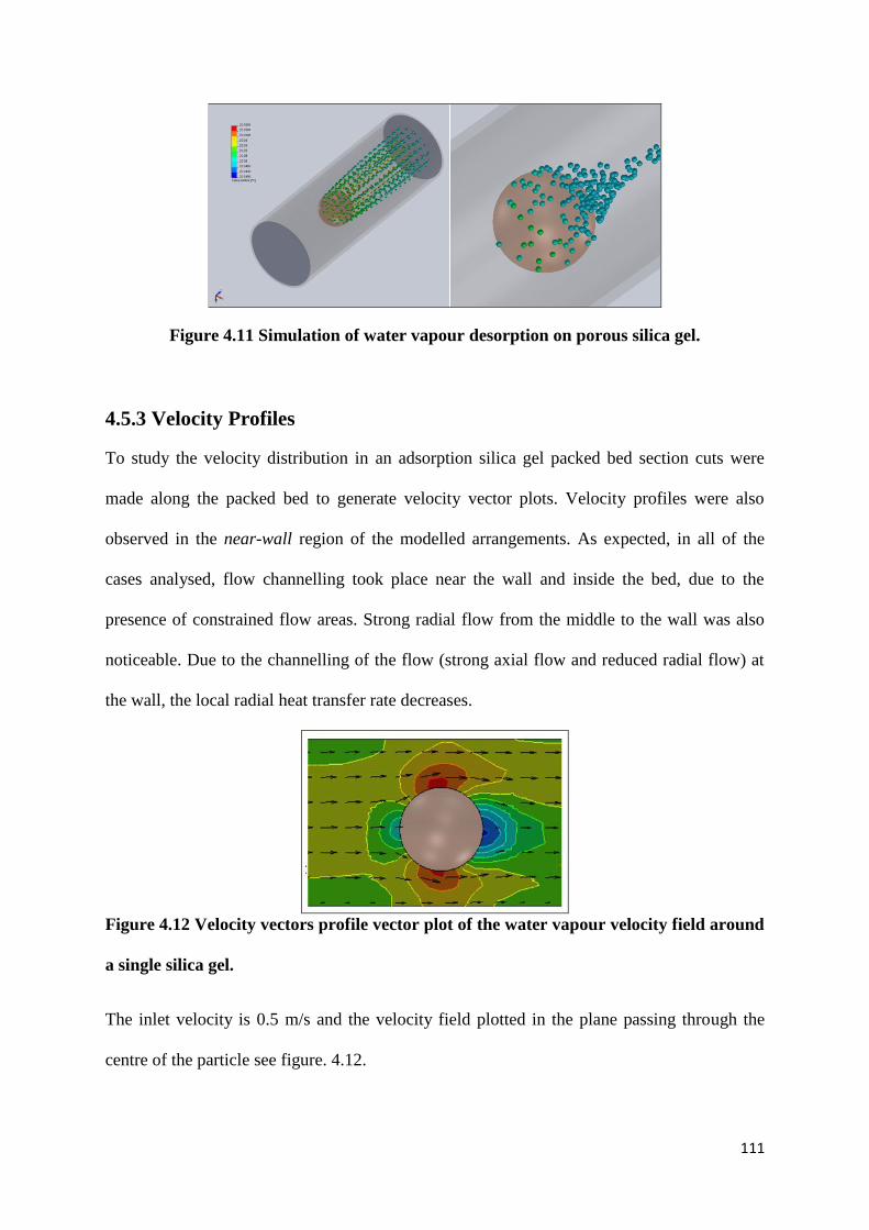
111
Figure 4.11 Simulation of water vapour desorption on porous silica gel.
4.5.3 Velocity Profiles
To study the velocity distribution in an adsorption silica gel packed bed section cuts were
made along the packed bed to generate velocity vector plots. Velocity profiles were also
observed in the near-wall region of the modelled arrangements. As expected, in all of the
cases analysed, flow channelling took place near the wall and inside the bed, due to the
presence of constrained flow areas. Strong radial flow from the middle to the wall was also
noticeable. Due to the channelling of the flow (strong axial flow and reduced radial flow) at
the wall, the local radial heat transfer rate decreases.
Figure 4.12 Velocity vectors profile vector plot of the water vapour velocity field around
a single silica gel.
The inlet velocity is 0.5 m/s and the velocity field plotted in the plane passing through the
centre of the particle see figure. 4.12.
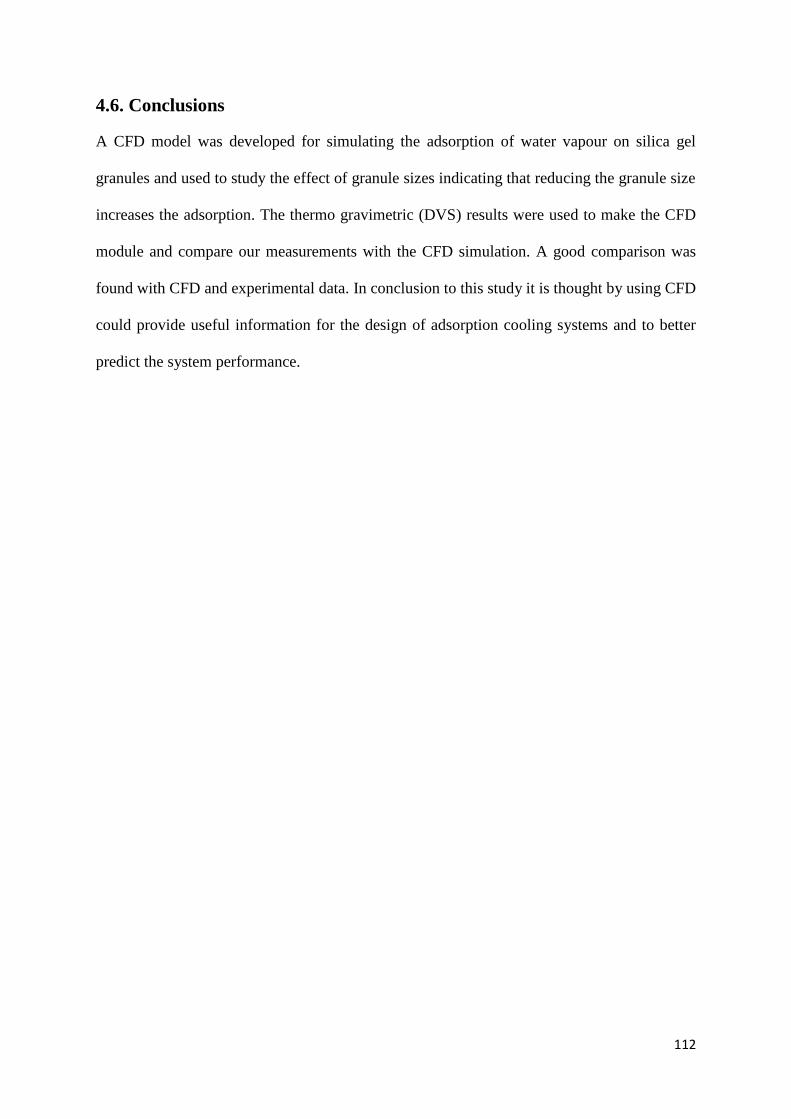
112
4.6. Conclusions
A CFD model was developed for simulating the adsorption of water vapour on silica gel
granules and used to study the effect of granule sizes indicating that reducing the granule size
increases the adsorption. The thermo gravimetric (DVS) results were used to make the CFD
module and compare our measurements with the CFD simulation. A good comparison was
found with CFD and experimental data. In conclusion to this study it is thought by using CFD
could provide useful information for the design of adsorption cooling systems and to better
predict the system performance.
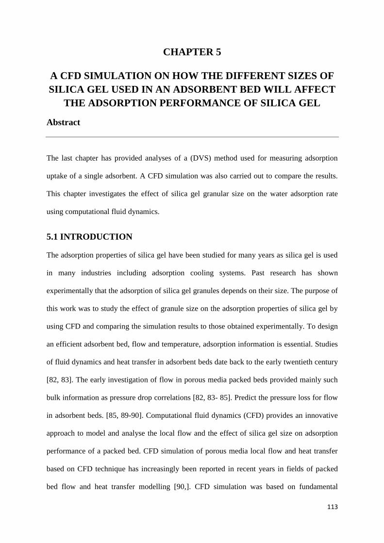
113
CHAPTER 5
A CFD SIMULATION ON HOW THE DIFFERENT SIZES OF
SILICA GEL USED IN AN ADSORBENT BED WILL AFFECT
THE ADSORPTION PERFORMANCE OF SILICA GEL
Abstract
The last chapter has provided analyses of a (DVS) method used for measuring adsorption
uptake of a single adsorbent. A CFD simulation was also carried out to compare the results.
This chapter investigates the effect of silica gel granular size on the water adsorption rate
using computational fluid dynamics.
5.1 INTRODUCTION
The adsorption properties of silica gel have been studied for many years as silica gel is used
in many industries including adsorption cooling systems. Past research has shown
experimentally that the adsorption of silica gel granules depends on their size. The purpose of
this work was to study the effect of granule size on the adsorption properties of silica gel by
using CFD and comparing the simulation results to those obtained experimentally. To design
an efficient adsorbent bed, flow and temperature, adsorption information is essential. Studies
of fluid dynamics and heat transfer in adsorbent beds date back to the early twentieth century
[82, 83]. The early investigation of flow in porous media packed beds provided mainly such
bulk information as pressure drop correlations [82, 83- 85]. Predict the pressure loss for flow
in adsorbent beds. [85, 89-90]. Computational fluid dynamics (CFD) provides an innovative
approach to model and analyse the local flow and the effect of silica gel size on adsorption
performance of a packed bed. CFD simulation of porous media local flow and heat transfer
based on CFD technique has increasingly been reported in recent years in fields of packed
bed flow and heat transfer modelling [90,]. CFD simulation was based on fundamental
114
principles of diffusion and adsorption/desorption of porous materials. In this study an
integrated CFD model was developed to model and simulate the adsorption dynamics of
water vapour in three different sizes of silica gel in a fixed bed adsorption column.
The developed integrated model was used to determine the adsorption capacity of the three
silica gel size type over a function of time, based on different operating conditions. The
simulated results were compared with past research papers experimental data and found to
give a good agreement. The effect of various influencing parameters such as velocity and
silica gel porosity were studied to investigate their influences on the adsorption capacity.
5.2 Methods
5.2.1 3D Geometry of silica gel packing
Geometric models of the silica gel adsorbent bed systems are generated for a tube of 25mm
length of 100 mm diameter.
The size of silica gel that is used in this CFD simulation is:
Silica gel granular size 1 mm
Silica gel granular size 2 mm
Silica gel granular size 3 mm
Adsorbent particle size affects how the water vapour flows through the adsorbent bed.
Smaller particles (higher mesh values) larger particles (lower mesh values).
First we selected the silica gel to particle sizes the silica gel were selected in the ranges of
40–60 mesh, 60–100 mesh, and 100–200 mesh.
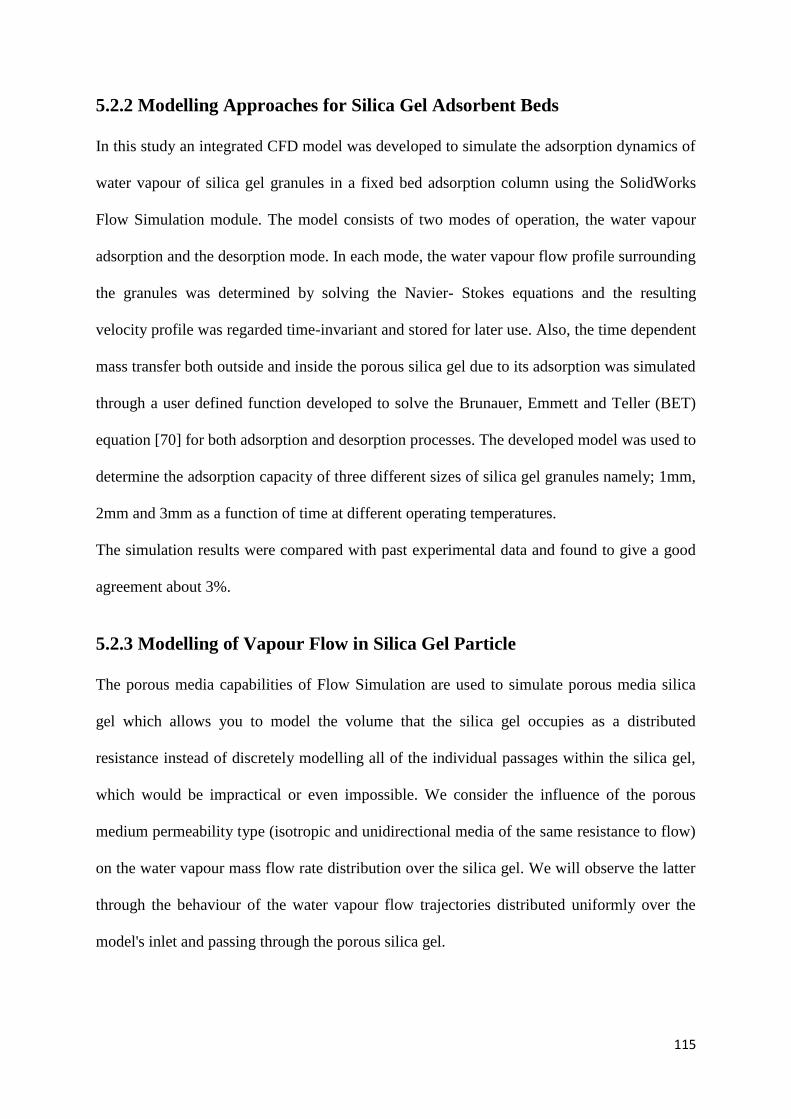
115
5.2.2 Modelling Approaches for Silica Gel Adsorbent Beds
In this study an integrated CFD model was developed to simulate the adsorption dynamics of
water vapour of silica gel granules in a fixed bed adsorption column using the SolidWorks
Flow Simulation module. The model consists of two modes of operation, the water vapour
adsorption and the desorption mode. In each mode, the water vapour flow profile surrounding
the granules was determined by solving the Navier- Stokes equations and the resulting
velocity profile was regarded time-invariant and stored for later use. Also, the time dependent
mass transfer both outside and inside the porous silica gel due to its adsorption was simulated
through a user defined function developed to solve the Brunauer, Emmett and Teller (BET)
equation [70] for both adsorption and desorption processes. The developed model was used to
determine the adsorption capacity of three different sizes of silica gel granules namely; 1mm,
2mm and 3mm as a function of time at different operating temperatures.
The simulation results were compared with past experimental data and found to give a good
agreement about 3%.
5.2.3 Modelling of Vapour Flow in Silica Gel Particle
The porous media capabilities of Flow Simulation are used to simulate porous media silica
gel which allows you to model the volume that the silica gel occupies as a distributed
resistance instead of discretely modelling all of the individual passages within the silica gel,
which would be impractical or even impossible. We consider the influence of the porous
medium permeability type (isotropic and unidirectional media of the same resistance to flow)
on the water vapour mass flow rate distribution over the silica gel. We will observe the latter
through the behaviour of the water vapour flow trajectories distributed uniformly over the
model's inlet and passing through the porous silica gel.
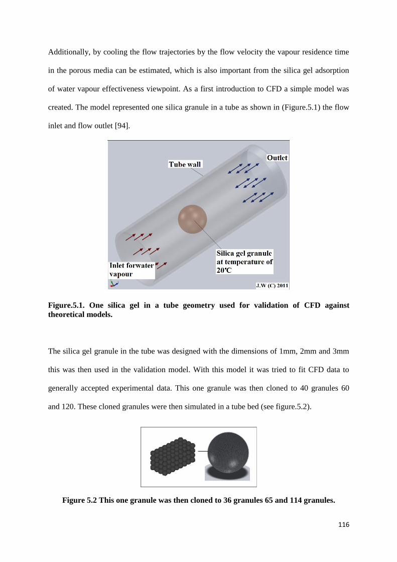
116
Additionally, by cooling the flow trajectories by the flow velocity the vapour residence time
in the porous media can be estimated, which is also important from the silica gel adsorption
of water vapour effectiveness viewpoint. As a first introduction to CFD a simple model was
created. The model represented one silica granule in a tube as shown in (Figure.5.1) the flow
inlet and flow outlet [94].
Figure.5.1. One silica gel in a tube geometry used for validation of CFD against
theoretical models.
The silica gel granule in the tube was designed with the dimensions of 1mm, 2mm and 3mm
this was then used in the validation model. With this model it was tried to fit CFD data to
generally accepted experimental data. This one granule was then cloned to 40 granules 60
and 120. These cloned granules were then simulated in a tube bed (see figure.5.2).
Figure 5.2 This one granule was then cloned to 36 granules 65 and 114 granules.
117
This limitation of granules was necessary to keep the model reasonable in size with a mesh
density comparable to the validation model. A series of runs was conducted at a number of
flow velocities see Table 5.3. In all these runs the centrally located granules had a defined
temperature of 20°C. The tube wall temperature was set at 20.5°C to create a 0.5°C
temperature difference between the granule and the fluid at infinite distance. The water
vapour that flowed through the tube was defined at 20°C at the entrance. The temperature of
the granules was simulated and recorded.
A constant diffusion coefficient De was assumed according to the reference of Sakoda et al.
[13]. The spherical silica gel particle with initial conditions of water content m(r) = 0 and a
temperature Tin is instantaneously exposed to vapour flow. The diffusion equation in the
silica gel particle is
(
) (5.1)
The initial condition and boundary conditions for equation (5.1) are
( )
( ) ( ) (5.2)
The mr is local water content of a silica gel particle in the radial direction and the me is the
equilibrium water content on the particle surface. The water content averaged in a silica gel
particle is given by
∫ (
) (5.3)
118
Where the porosity in a silica gel particle was fixed at ep = 0.38 for 1mm silica gel, 0.38 for
2mm silica gel and 0.34 for the 3mm silica gel.
5.3 CFD Governing Equations
The transport phenomena can be divided into adsorption and water vapour flow in the
adsorber bed, silica gel granules surfaces Navier-Stokes equations for flow are used to solve
the water vapour flow phase:[1,91,94]
(5.4)
The p represents pressure, η dynamic viscosity and density of the fluid the flow velocity
can be simulated in first. This simulated data is then stored and used for solving the
convection-diffusion equation.[1]
(5.5)
The c represents the water vapour molecule adsorbed into the silica gel, and D the diffusion
flow coefficient in the silica gel. In contrast to diffusion, an effective diffusivity De must be
applied [1,91,94]:
(5.6)
The cp represents the water vapour molecule adsorbed within the silica gel particle. The mass
transfer resistance between the silica gel surface is also modelled.[1]
119
(
) ( )
(
) ( ) (5.7)
The represents the normal vector of the outer silica surface. The driving force of transport
over the particle boundary is relative to the adsorption difference, and kf is the corresponding
mass transfer coefficient. The adsorbent beds in the CFD simulation are simulated with far
less
silica gel granules than in a real adsorbent bed. In order to simulate similar systems, the
effective diffusivity De is increased. The adsorption of the water vapour molecules at the
silica surfaces is described by a classical Langmuir-type kinetic:[1,91-93].
( ) (5.8)
The ka and kd represents adsorption and desorption rates, q max maximum capacity, and q the
current occupation of binding sites at the surface.
5.3.1 Desorption of Vapour in Porous Materials
When considering desorption in a porous material one must considers vapour transport the
Lattice Boltzmann equation can be expressed as:
( ) (5.9)
This can be done with Lattice Boltzmann multi physics extension by applying a local rule
describing the change of the adsorption rate on the water vapour concentration C and
the adsorbed mass S deposited per unit volume of the porous media matrix.
With parameters and exponents fulfilling At equilibrium, i.e. for
this model reduces to a Freundlich isotherm:[91,93-94].
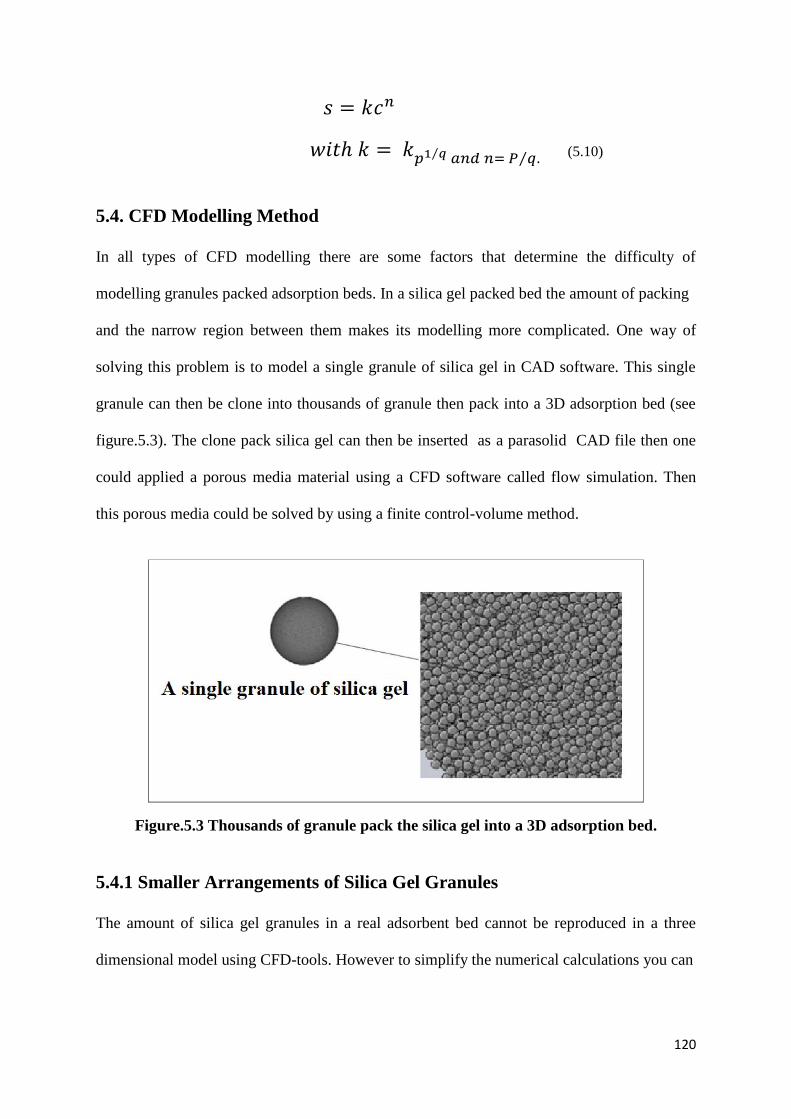
120
⁄ ⁄ (5.10)
5.4. CFD Modelling Method
In all types of CFD modelling there are some factors that determine the difficulty of
modelling granules packed adsorption beds. In a silica gel packed bed the amount of packing
and the narrow region between them makes its modelling more complicated. One way of
solving this problem is to model a single granule of silica gel in CAD software. This single
granule can then be clone into thousands of granule then pack into a 3D adsorption bed (see
figure.5.3). The clone pack silica gel can then be inserted as a parasolid CAD file then one
could applied a porous media material using a CFD software called flow simulation. Then
this porous media could be solved by using a finite control-volume method.
Figure.5.3 Thousands of granule pack the silica gel into a 3D adsorption bed.
5.4.1 Smaller Arrangements of Silica Gel Granules
The amount of silica gel granules in a real adsorbent bed cannot be reproduced in a three
dimensional model using CFD-tools. However to simplify the numerical calculations you can
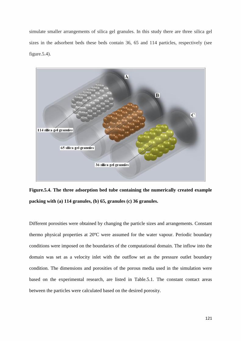
121
simulate smaller arrangements of silica gel granules. In this study there are three silica gel
sizes in the adsorbent beds these beds contain 36, 65 and 114 particles, respectively (see
figure.5.4).
Figure.5.4. The three adsorption bed tube containing the numerically created example
packing with (a) 114 granules, (b) 65, granules (c) 36 granules.
Different porosities were obtained by changing the particle sizes and arrangements. Constant
thermo physical properties at 20ºC were assumed for the water vapour. Periodic boundary
conditions were imposed on the boundaries of the computational domain. The inflow into the
domain was set as a velocity inlet with the outflow set as the pressure outlet boundary
condition. The dimensions and porosities of the porous media used in the simulation were
based on the experimental research, are listed in Table.5.1. The constant contact areas
between the particles were calculated based on the desired porosity.
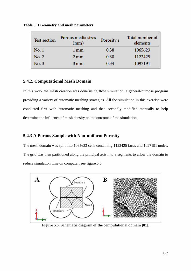
122
Table.5. 1 Geometry and mesh parameters
5.4.2. Computational Mesh Domain
In this work the mesh creation was done using flow simulation, a general-purpose program
providing a variety of automatic meshing strategies. All the simulation in this exercise were
conducted first with automatic meshing and then secondly modified manually to help
determine the influence of mesh density on the outcome of the simulation.
5.4.3 A Porous Sample with Non-uniform Porosity
The mesh domain was split into 1065623 cells containing 1122425 faces and 1097191 nodes.
The grid was then partitioned along the principal axis into 3 segments to allow the domain to
reduce simulation time on computer, see figure.5.5
Figure 5.5. Schematic diagram of the computational domain [81].
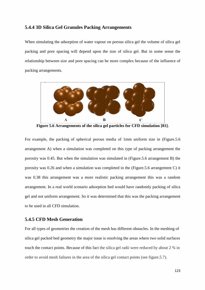
123
5.4.4 3D Silica Gel Granules Packing Arrangements
When simulating the adsorption of water vapour on porous silica gel the volume of silica gel
packing and pore spacing will depend upon the size of silica gel. But in some sense the
relationship between size and pore spacing can be more complex because of the influence of
packing arrangements.
Figure 5.6 Arrangements of the silica gel particles for CFD simulation [81].
For example, the packing of spherical porous media of 1mm uniform size in (Figure.5.6
arrangement A) when a simulation was completed on this type of packing arrangement the
porosity was 0.45. But when the simulation was simulated in (Figure.5.6 arrangement B) the
porosity was 0.26 and when a simulation was completed in the (Figure.5.6 arrangement C) it
was 0.38 this arrangement was a more realistic packing arrangement this was a random
arrangement. In a real world scenario adsorption bed would have randomly packing of silica
gel and not uniform arrangement. So it was determined that this was the packing arrangement
to be used in all CFD simulation.
5.4.5 CFD Mesh Generation
For all types of geometries the creation of the mesh has different obstacles. In the meshing of
silica gel packed bed geometry the major issue is resolving the areas where two solid surfaces
touch the contact points. Because of this fact the silica gel radii were reduced by about 2 % in
order to avoid mesh failures in the area of the silica gel contact points (see figure.5.7).
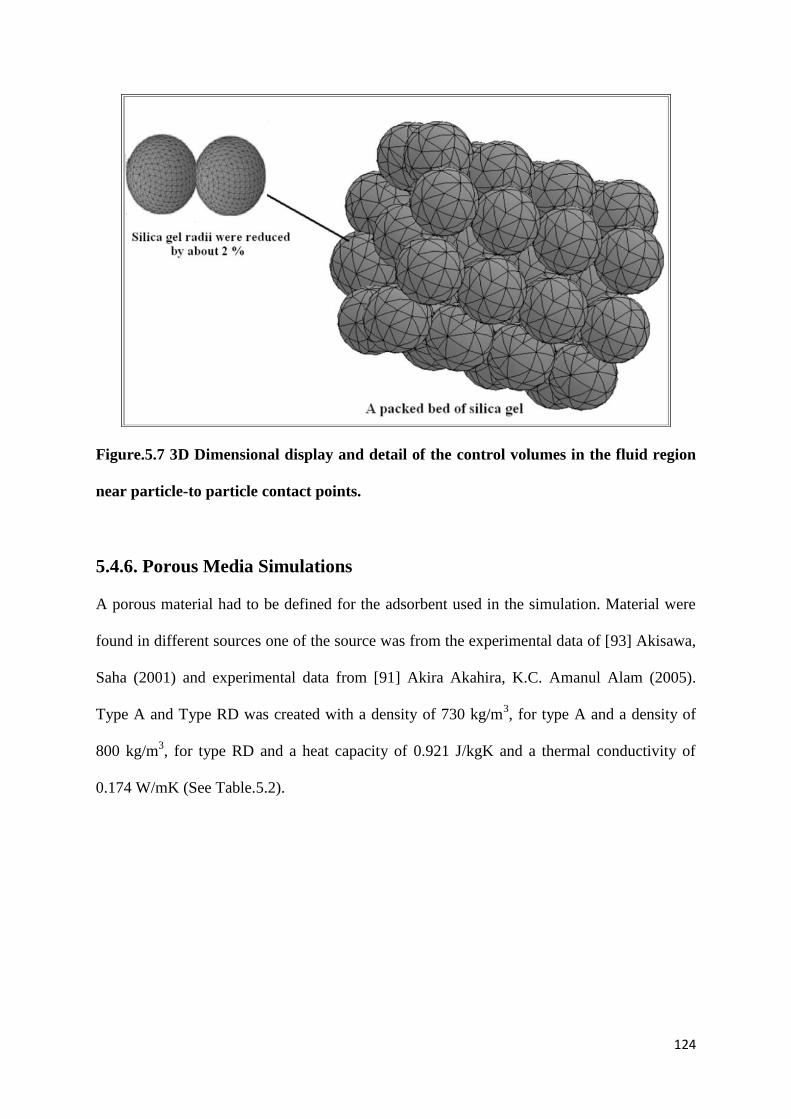
124
Figure.5.7 3D Dimensional display and detail of the control volumes in the fluid region
near particle-to particle contact points.
5.4.6. Porous Media Simulations
A porous material had to be defined for the adsorbent used in the simulation. Material were
found in different sources one of the source was from the experimental data of [93] Akisawa,
Saha (2001) and experimental data from [91] Akira Akahira, K.C. Amanul Alam (2005).
Type A and Type RD was created with a density of 730 kg/m3, for type A and a density of
800 kg/m3, for type RD and a heat capacity of 0.921 J/kgK and a thermal conductivity of
0.174 W/mK (See Table.5.2).
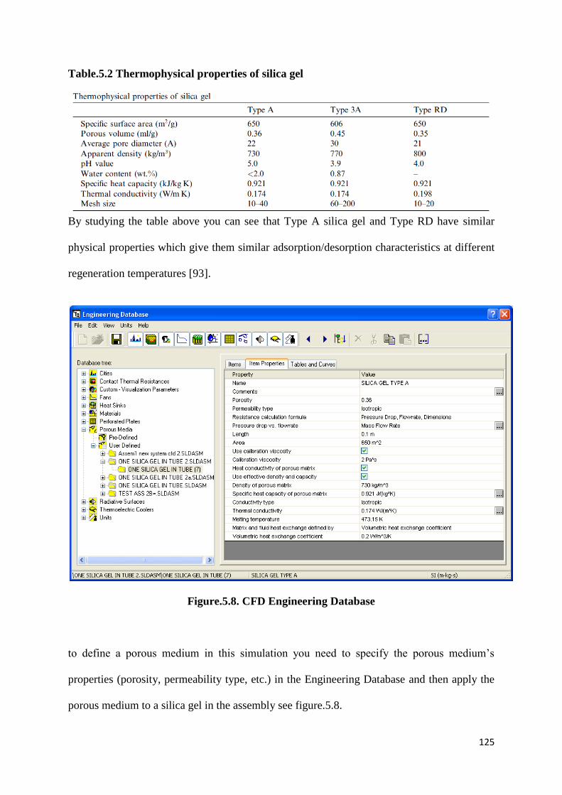
125
Table.5.2 Thermophysical properties of silica gel
By studying the table above you can see that Type A silica gel and Type RD have similar
physical properties which give them similar adsorption/desorption characteristics at different
regeneration temperatures [93].
Figure.5.8. CFD Engineering Database
to define a porous medium in this simulation you need to specify the porous medium’s
properties (porosity, permeability type, etc.) in the Engineering Database and then apply the
porous medium to a silica gel in the assembly see figure.5.8.
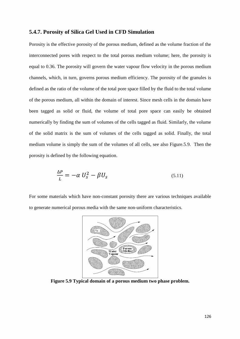
126
5.4.7. Porosity of Silica Gel Used in CFD Simulation
Porosity is the effective porosity of the porous medium, defined as the volume fraction of the
interconnected pores with respect to the total porous medium volume; here, the porosity is
equal to 0.36. The porosity will govern the water vapour flow velocity in the porous medium
channels, which, in turn, governs porous medium efficiency. The porosity of the granules is
defined as the ratio of the volume of the total pore space filled by the fluid to the total volume
of the porous medium, all within the domain of interest. Since mesh cells in the domain have
been tagged as solid or fluid, the volume of total pore space can easily be obtained
numerically by finding the sum of volumes of the cells tagged as fluid. Similarly, the volume
of the solid matrix is the sum of volumes of the cells tagged as solid. Finally, the total
medium volume is simply the sum of the volumes of all cells, see also Figure.5.9. Then the
porosity is defined by the following equation.
(5.11)
For some materials which have non-constant porosity there are various techniques available
to generate numerical porous media with the same non-uniform characteristics.
Figure 5.9 Typical domain of a porous medium two phase problem.
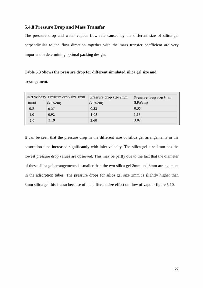
127
5.4.8 Pressure Drop and Mass Transfer
The pressure drop and water vapour flow rate caused by the different size of silica gel
perpendicular to the flow direction together with the mass transfer coefficient are very
important in determining optimal packing design.
Table 5.3 Shows the pressure drop for different simulated silica gel size and
arrangement.
It can be seen that the pressure drop in the different size of silica gel arrangements in the
adsorption tube increased significantly with inlet velocity. The silica gel size 1mm has the
lowest pressure drop values are observed. This may be partly due to the fact that the diameter
of these silica gel arrangements is smaller than the two silica gel 2mm and 3mm arrangement
in the adsorption tubes. The pressure drops for silica gel size 2mm is slightly higher than
3mm silica gel this is also because of the different size effect on flow of vapour figure 5.10.
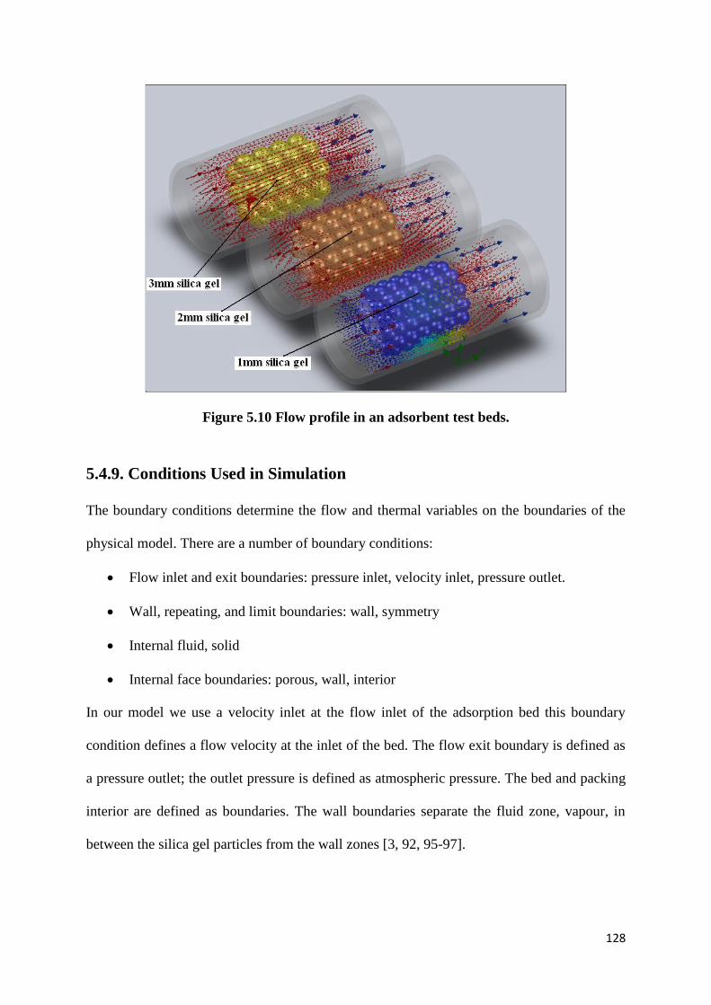
128
Figure 5.10 Flow profile in an adsorbent test beds.
5.4.9. Conditions Used in Simulation
The boundary conditions determine the flow and thermal variables on the boundaries of the
physical model. There are a number of boundary conditions:
Flow inlet and exit boundaries: pressure inlet, velocity inlet, pressure outlet.
Wall, repeating, and limit boundaries: wall, symmetry
Internal fluid, solid
Internal face boundaries: porous, wall, interior
In our model we use a velocity inlet at the flow inlet of the adsorption bed this boundary
condition defines a flow velocity at the inlet of the bed. The flow exit boundary is defined as
a pressure outlet; the outlet pressure is defined as atmospheric pressure. The bed and packing
interior are defined as boundaries. The wall boundaries separate the fluid zone, vapour, in
between the silica gel particles from the wall zones [3, 92, 95-97].
129
With the determination of the boundary conditions the physical model has been defined and a
numerical solution can be provided. It was then necessary to determine how the solution will
be established. This was be done by setting the iteration parameters. With all boundary
conditions defined, a number of additional parameters and solving schemes where selected.
An initial condition was assigned to the model and was used to help speed the convergence of
the computation. The computation is an iterative process that solves the governing equations
for flow and energy in each simulated cell. Depending on the complexity of the model and
the computer resources available, CFD simulation can take anywhere from minutes to days
[10]. The results of the simulation can be viewed and manipulated with post-processing
software once the simulation has converted to a solution [98-100].
5.4.10. Fluid Flow Fundamentals
For iteration CFD solvers use generalized fluid flow and energy balances based on the
Navier- Stokes equations. The balances are generalized so the user can influence which
elements are added in the balance and which are not. The number of balances to be solved is
also user defined; it can be advantageous to not solve all balances initially. The generalized
balances that are used by the Flow simulation commercial CFD package are the Navier-
Stokes equations for conservation of mass and momentum, when it is set to calculate laminar
flow without heat transfer. Additional equations are solved for heat transfer, species mixing
or reaction or and for turbulent cases [99].
5.5. Results and Discussion
The present CFD simulation attempt to clarify the adsorption characteristics of the adsorption
bed packed with spherical silica gel type A under the boundary condition of parameters such
as a width of packed bed, the inlet water vapour velocity and granule size of silica gel[89].
130
5.5.1. Granules Packing Gap Between Walls
To be able to solve for turbulent flow in a CFD simulation it was necessary to introduce a
small gap between the wall and the silica gel granules. It was shown from comparisons of
flow profiles at several gap sizes that the small gaps used in the final model did not affect the
stagnant flow area around the contact points. Rahimi, M. and Mohseni, M (2008) [3].
5.6. CFD Validation against DVS Experimental Results
The CFD simulation model has been used to simulate the water vapour adsorption and
desorption onto silica gel porous media, heat transfer and velocity. The results simulated
using the CFD model, were compared with the experimental DVS results. Based on the
simulation results, the data demonstrated a good agreement with the experimental data. Based
on the comparison of the experimental results and CFD simulation several important
operating parameters were verified.
5.6.1 Velocity Profiles
In all CFD simulation it was notice that the water vapour flow in the middle of the porous
media granules and the wall channel as expected Rahimi, M. and Mohseni, M (2008) [3]. It
was also noticed that velocity increased by the inlet and velocity in some constrained areas of
the adsorption bed. Stagnation points and secondary flows were also noticed near the contact
points Figure.5.11.
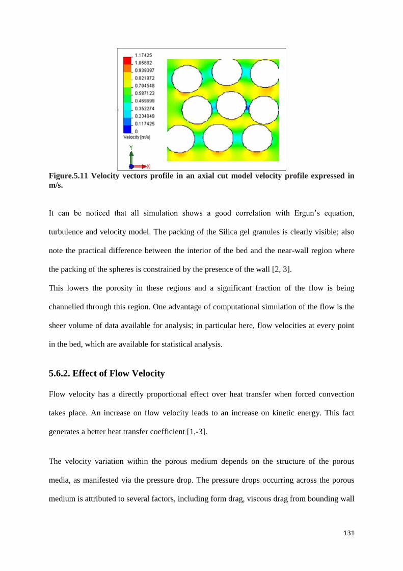
131
Figure.5.11 Velocity vectors profile in an axial cut model velocity profile expressed in
m/s.
It can be noticed that all simulation shows a good correlation with Ergun’s equation,
turbulence and velocity model. The packing of the Silica gel granules is clearly visible; also
note the practical difference between the interior of the bed and the near-wall region where
the packing of the spheres is constrained by the presence of the wall [2, 3].
This lowers the porosity in these regions and a significant fraction of the flow is being
channelled through this region. One advantage of computational simulation of the flow is the
sheer volume of data available for analysis; in particular here, flow velocities at every point
in the bed, which are available for statistical analysis.
5.6.2. Effect of Flow Velocity
Flow velocity has a directly proportional effect over heat transfer when forced convection
takes place. An increase on flow velocity leads to an increase on kinetic energy. This fact
generates a better heat transfer coefficient [1,-3].
The velocity variation within the porous medium depends on the structure of the porous
media, as manifested via the pressure drop. The pressure drops occurring across the porous
medium is attributed to several factors, including form drag, viscous drag from bounding wall
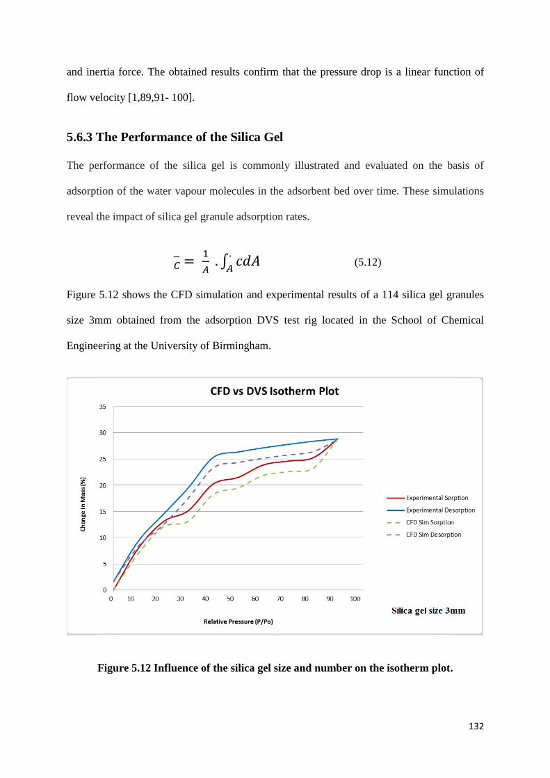
132
and inertia force. The obtained results confirm that the pressure drop is a linear function of
flow velocity [1,89,91- 100].
5.6.3 The Performance of the Silica Gel
The performance of the silica gel is commonly illustrated and evaluated on the basis of
adsorption of the water vapour molecules in the adsorbent bed over time. These simulations
reveal the impact of silica gel granule adsorption rates.
∫
(5.12)
Figure 5.12 shows the CFD simulation and experimental results of a 114 silica gel granules
size 3mm obtained from the adsorption DVS test rig located in the School of Chemical
Engineering at the University of Birmingham.
Figure 5.12 Influence of the silica gel size and number on the isotherm plot.
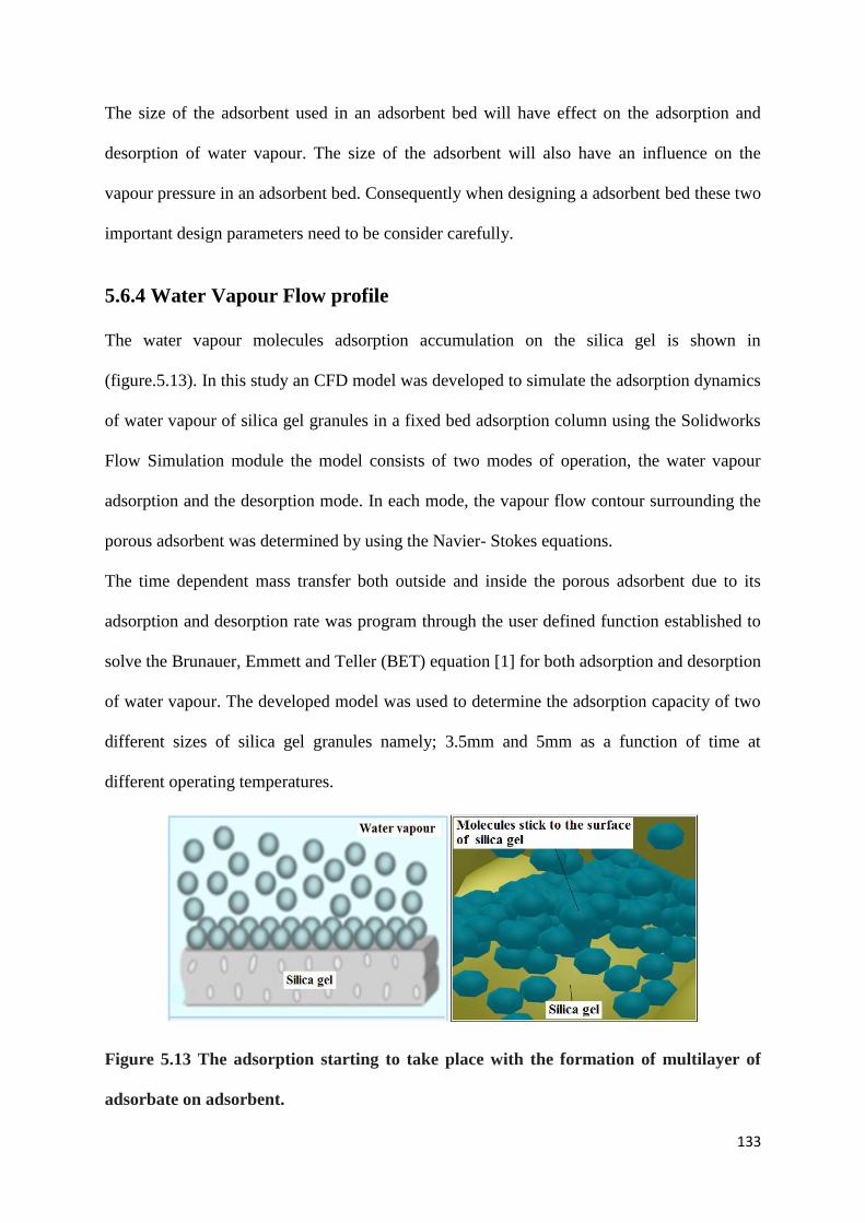
133
The size of the adsorbent used in an adsorbent bed will have effect on the adsorption and
desorption of water vapour. The size of the adsorbent will also have an influence on the
vapour pressure in an adsorbent bed. Consequently when designing a adsorbent bed these two
important design parameters need to be consider carefully.
5.6.4 Water Vapour Flow profile
The water vapour molecules adsorption accumulation on the silica gel is shown in
(figure.5.13). In this study an CFD model was developed to simulate the adsorption dynamics
of water vapour of silica gel granules in a fixed bed adsorption column using the Solidworks
Flow Simulation module the model consists of two modes of operation, the water vapour
adsorption and the desorption mode. In each mode, the vapour flow contour surrounding the
porous adsorbent was determined by using the Navier- Stokes equations.
The time dependent mass transfer both outside and inside the porous adsorbent due to its
adsorption and desorption rate was program through the user defined function established to
solve the Brunauer, Emmett and Teller (BET) equation [1] for both adsorption and desorption
of water vapour. The developed model was used to determine the adsorption capacity of two
different sizes of silica gel granules namely; 3.5mm and 5mm as a function of time at
different operating temperatures.
Figure 5.13 The adsorption starting to take place with the formation of multilayer of
adsorbate on adsorbent.
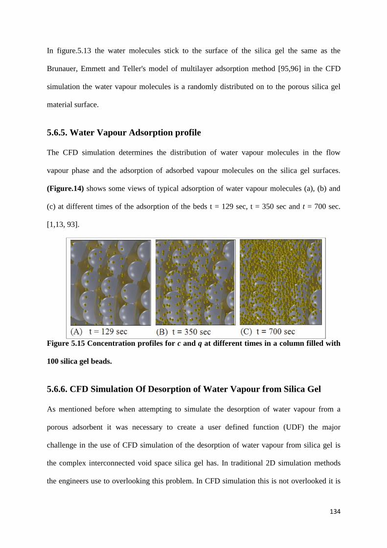
134
In figure.5.13 the water molecules stick to the surface of the silica gel the same as the
Brunauer, Emmett and Teller's model of multilayer adsorption method [95,96] in the CFD
simulation the water vapour molecules is a randomly distributed on to the porous silica gel
material surface.
5.6.5. Water Vapour Adsorption profile
The CFD simulation determines the distribution of water vapour molecules in the flow
vapour phase and the adsorption of adsorbed vapour molecules on the silica gel surfaces.
(Figure.14) shows some views of typical adsorption of water vapour molecules (a), (b) and
(c) at different times of the adsorption of the beds t = 129 sec, t = 350 sec and t = 700 sec.
[1,13, 93].
Figure 5.15 Concentration profiles for c and q at different times in a column filled with
100 silica gel beads.
5.6.6. CFD Simulation Of Desorption of Water Vapour from Silica Gel
As mentioned before when attempting to simulate the desorption of water vapour from a
porous adsorbent it was necessary to create a user defined function (UDF) the major
challenge in the use of CFD simulation of the desorption of water vapour from silica gel is
the complex interconnected void space silica gel has. In traditional 2D simulation methods
the engineers use to overlooking this problem. In CFD simulation this is not overlooked it is
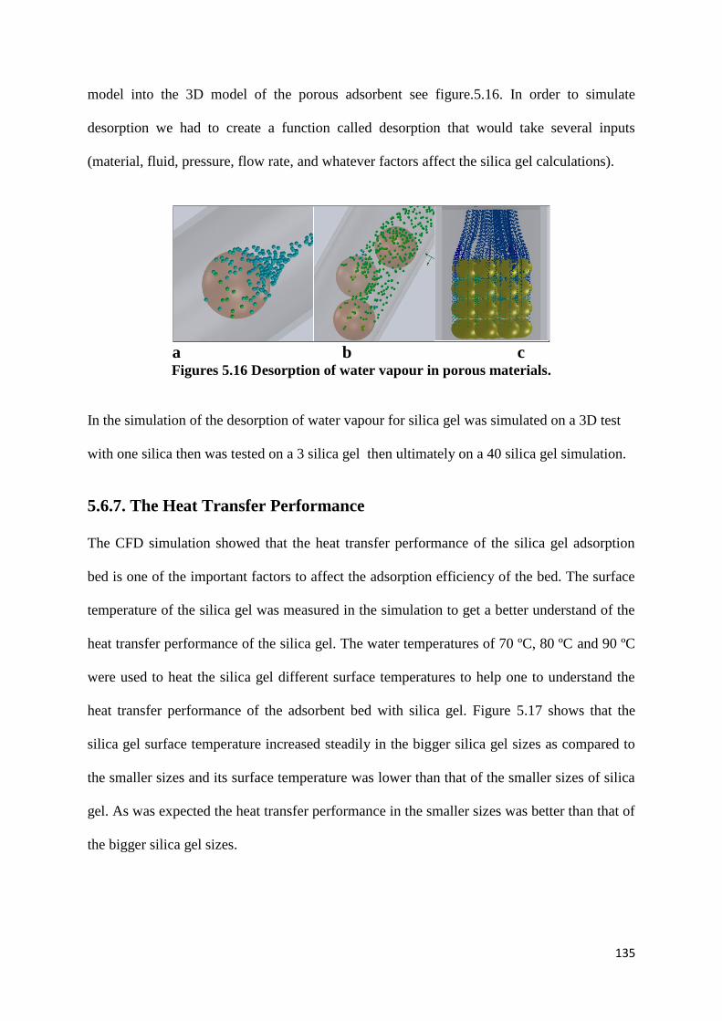
135
model into the 3D model of the porous adsorbent see figure.5.16. In order to simulate
desorption we had to create a function called desorption that would take several inputs
(material, fluid, pressure, flow rate, and whatever factors affect the silica gel calculations).
a b c
Figures 5.16 Desorption of water vapour in porous materials.
In the simulation of the desorption of water vapour for silica gel was simulated on a 3D test
with one silica then was tested on a 3 silica gel then ultimately on a 40 silica gel simulation.
5.6.7. The Heat Transfer Performance
The CFD simulation showed that the heat transfer performance of the silica gel adsorption
bed is one of the important factors to affect the adsorption efficiency of the bed. The surface
temperature of the silica gel was measured in the simulation to get a better understand of the
heat transfer performance of the silica gel. The water temperatures of 70 ºC, 80 ºC and 90 ºC
were used to heat the silica gel different surface temperatures to help one to understand the
heat transfer performance of the adsorbent bed with silica gel. Figure 5.17 shows that the
silica gel surface temperature increased steadily in the bigger silica gel sizes as compared to
the smaller sizes and its surface temperature was lower than that of the smaller sizes of silica
gel. As was expected the heat transfer performance in the smaller sizes was better than that of
the bigger silica gel sizes.

136
Figure 5.17 The variation of the surface temperature of silica gel size with the heating
time.
5.7 Conclusions
A CFD model was developed for simulating the adsorption of water vapour on silica gel
granules and used to study the effect of granule sizes indicating that reducing the granule size
increases the adsorption. It can be concluded that CFD is a promising tool in evaluating heat
transfer behaviour in an adsorption bed. Further CFD studies, with a larger silica gel and
porous media, are required in the future simulation to show whether they will produce the
same results.
137
CHAPTER 6
CFD SIMULATION OF TWO DIFFERENT DESIGN
CONFIGURATIONS OF HEAT EXCHANGER USED IN
ADSORBENT BED AS PART OF AN ADSORPTION
COOLING SYSTEM
Abstract
The performance of the adsorption cooling system is assessed in terms of the heat transfer
coefficients of adsorbent bed heat exchanger. These parameters in-turn determine the specific
cooling capacity (SCC) and the coefficient of the performance (COP) of the adsorption
cooling system. It was observed that the overall heat transfer coefficients of the heat
exchanger have a direct linear relation with the hot water output temperatures.
6.1. Introduction
An Adsorption cooling system is promising technology since it incorporates environmentally
benign refrigerants and the industrial waste heat or low grade solar energy instead of
mechanical power. However the low value of performance parameters (COP and SCP), high
initial cost and the operating pressure, which is quite low these are the main issues that hold
back the widespread application of the adsorption cooling systems. One of the efficient ways
to improve the low SCP and COP of this system is the appropriate selection of the design and
operating parameters of an adsorbent bed. The heat exchanger used as part of the adsorption
system is one of the influential parameter in the heat transfer performance of an adsorption
cooling system.
Studies relevant to this research span the last few decades. Chang et.al (2005) [25]
experimental study that investigated the heat transfer efficiency of flat tube heat exchanger
concluded that the flat tube heat exchanger thinner improves the mass transfer performance
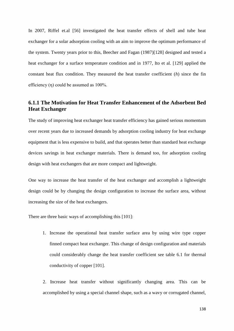
138
In 2007, Riffel et.al [56] investigated the heat transfer effects of shell and tube heat
exchanger for a solar adsorption cooling with an aim to improve the optimum performance of
the system. Twenty years prior to this, Beecher and Fagan (1987)[128] designed and tested a
heat exchanger for a surface temperature condition and in 1977, Ito et al. [129] applied the
constant heat flux condition. They measured the heat transfer coefficient (h) since the fin
efficiency (η) could be assumed as 100%.
6.1.1 The Motivation for Heat Transfer Enhancement of the Adsorbent Bed
Heat Exchanger The study of improving heat exchanger heat transfer efficiency has gained serious momentum
over recent years due to increased demands by adsorption cooling industry for heat exchange
equipment that is less expensive to build, and that operates better than standard heat exchange
devices savings in heat exchanger materials. There is demand too, for adsorption cooling
design with heat exchangers that are more compact and lightweight.
One way to increase the heat transfer of the heat exchanger and accomplish a lightweight
design could be by changing the design configuration to increase the surface area, without
increasing the size of the heat exchangers.
There are three basic ways of accomplishing this [101]:
1. Increase the operational heat transfer surface area by using wire type copper
finned compact heat exchanger. This change of design configuration and materials
could considerably change the heat transfer coefficient see table 6.1 for thermal
conductivity of copper [101].
2. Increase heat transfer without significantly changing area. This can be
accomplished by using a special channel shape, such as a wavy or corrugated channel,
139
which would provide mixing due to secondary flows and boundary-layer separation
within the channel. Vortex generators also increase heat transfer coefficient without a
significant area increase by creating longitudinally spiralling vortices exchange fluid
between the wall and core regions of the flow, resulting in increased heat transfer
[101].
3. Increase both heat transfer coefficient and surface area of a heat exchanger by.
Interrupted fins (i.e., offset strip and louvered fins) act in this way. These surfaces
increase the effective surface area, and enhance heat transfer through repeated growth
and destruction of the boundary layers [101].
The use of any one of these heat transfer method mentioned could substantially increase the
heat transfer fin efficiency and the motivation behind the design of new a adsorbent bed
compact copper wire woven heat exchanger.
6.1.2 The heat exchanger fin performance
Heat exchanger fin performance can be explained by two different methods. The first is fin
effectiveness this is the ratio of the heat exchanger fin heat transfer to the heat transfer of the
tube without fin [101]. The second is the fin efficiency and is defined as the ratio of the heat
transferred through the actual fin to that transferred through a perfect fin.
A perfect fin is thought to be one made of a perfect or infinite conductor material. A perfect
conductor has an infinite thermal conductivity, so in theory, the entire fin is at the base
material heat transfer temperature [54,101].
The equation for this is
, (6.1)
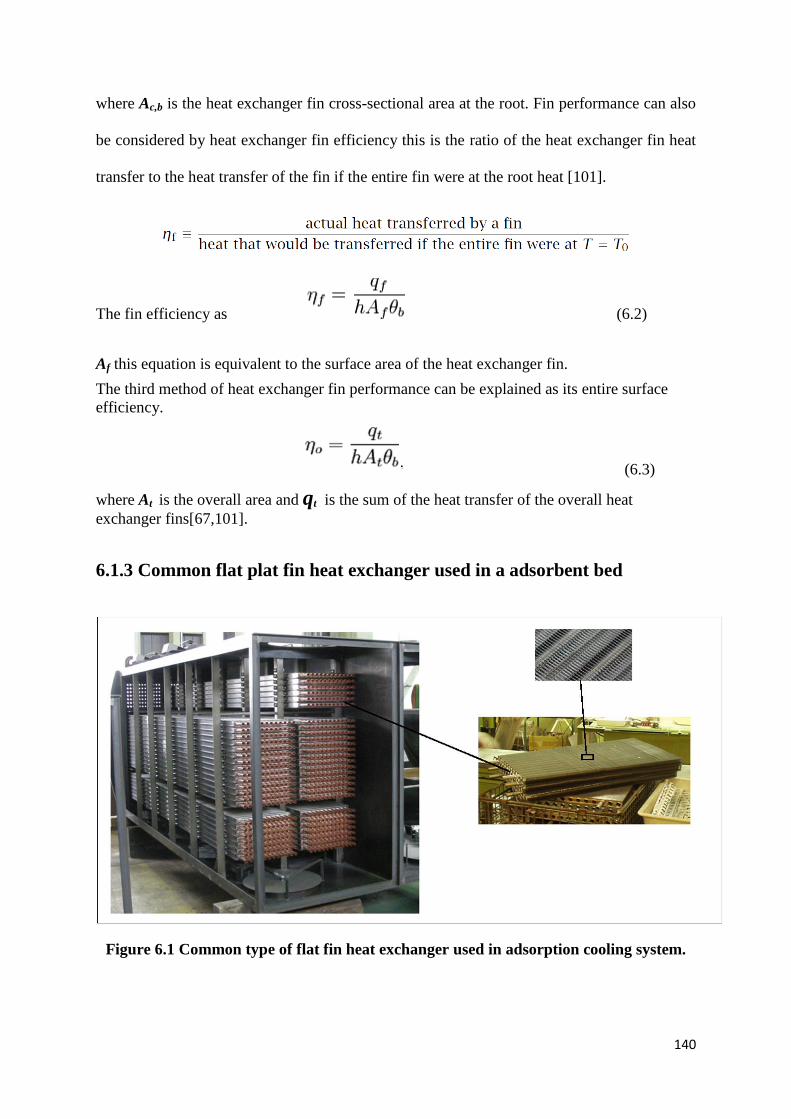
140
where Ac,b is the heat exchanger fin cross-sectional area at the root. Fin performance can also
be considered by heat exchanger fin efficiency this is the ratio of the heat exchanger fin heat
transfer to the heat transfer of the fin if the entire fin were at the root heat [101].
The fin efficiency as (6.2)
Af this equation is equivalent to the surface area of the heat exchanger fin.
The third method of heat exchanger fin performance can be explained as its entire surface
efficiency.
(6.3)
where At is the overall area and qt is the sum of the heat transfer of the overall heat
exchanger fins[67,101].
6.1.3 Common flat plat fin heat exchanger used in a adsorbent bed
Figure 6.1 Common type of flat fin heat exchanger used in adsorption cooling system.
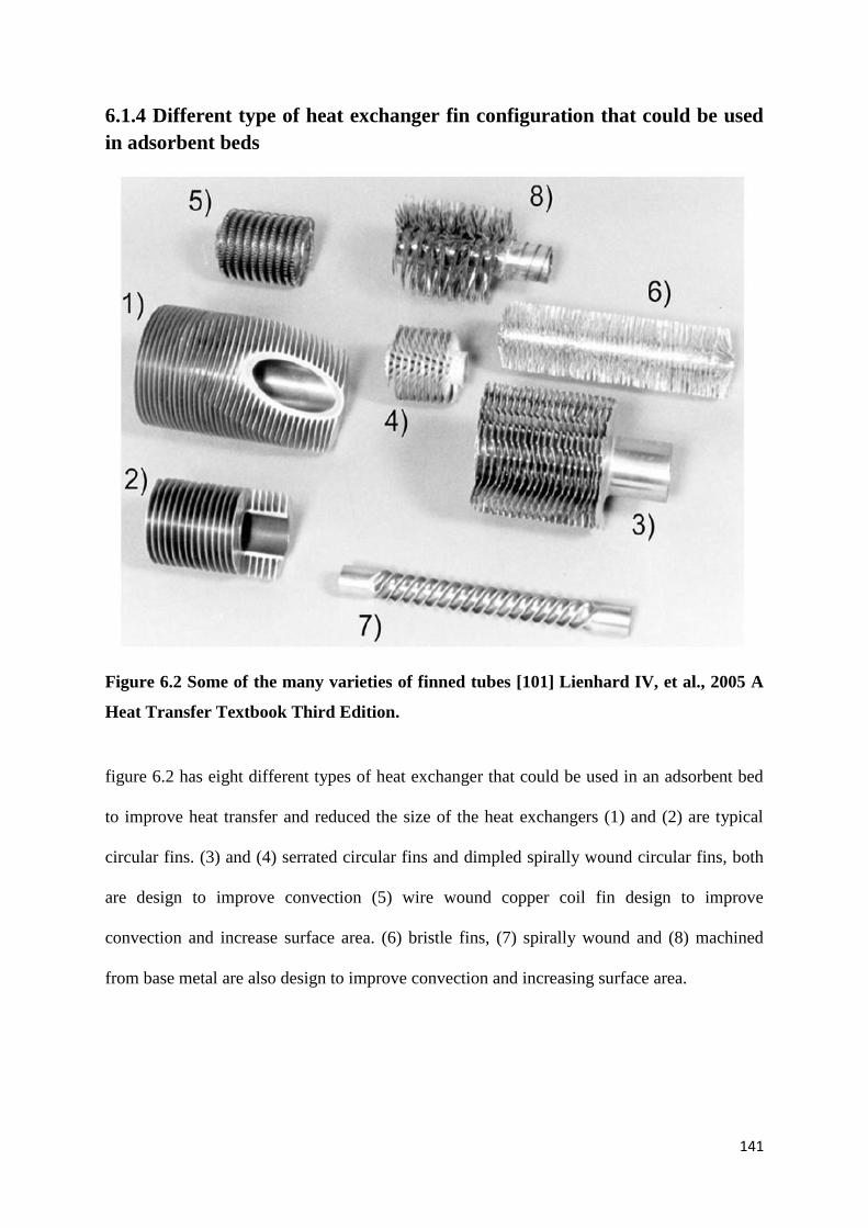
141
6.1.4 Different type of heat exchanger fin configuration that could be used
in adsorbent beds
Figure 6.2 Some of the many varieties of finned tubes [101] Lienhard IV, et al., 2005 A
Heat Transfer Textbook Third Edition.
figure 6.2 has eight different types of heat exchanger that could be used in an adsorbent bed
to improve heat transfer and reduced the size of the heat exchangers (1) and (2) are typical
circular fins. (3) and (4) serrated circular fins and dimpled spirally wound circular fins, both
are design to improve convection (5) wire wound copper coil fin design to improve
convection and increase surface area. (6) bristle fins, (7) spirally wound and (8) machined
from base metal are also design to improve convection and increasing surface area.
142
6.1.5 Comparison of aluminum flat fins heat exchangers to copper wire
woven fins heat exchanger
An important design aspect of adsorbent bed heat exchanger technology is deciding what
materials are appropriate for the design of adsorbent bed heat exchanger. The common choice
is aluminum alloy 1050A or 6063A flat fins. These types of aluminum have one of the
highest thermal conductivity values, see table 6.1. Thus is a good material for removing heat
from a system to an external environment. In the case of an adsorbent bed, the heat
exchanger is packed with porous adsorbent material and so the extended fins are used to
increase and decrease the heat transfer rate from the fluid inside the heat exchanger to the
surface of the porous adsorbent.
The porous adsorbent affects thermal conductivity of flat fins heat exchange. To overcome
this problem, the heat exchanger designers design the heat exchanger fins larger to improve
the heat transfer. This is one of the causes for the bulky size adsorption cooling system. One
way designers could solve this problem is by changing the material and design configuration
of the heat exchanger of the adsorbent bed.
In this chapter a copper wire woven fins heat exchanger is used for the adsorbent bed. Copper
has around twice the thermal conductivity of aluminium see table 6.1 for the properties of
copper heat exchangers materials [101].
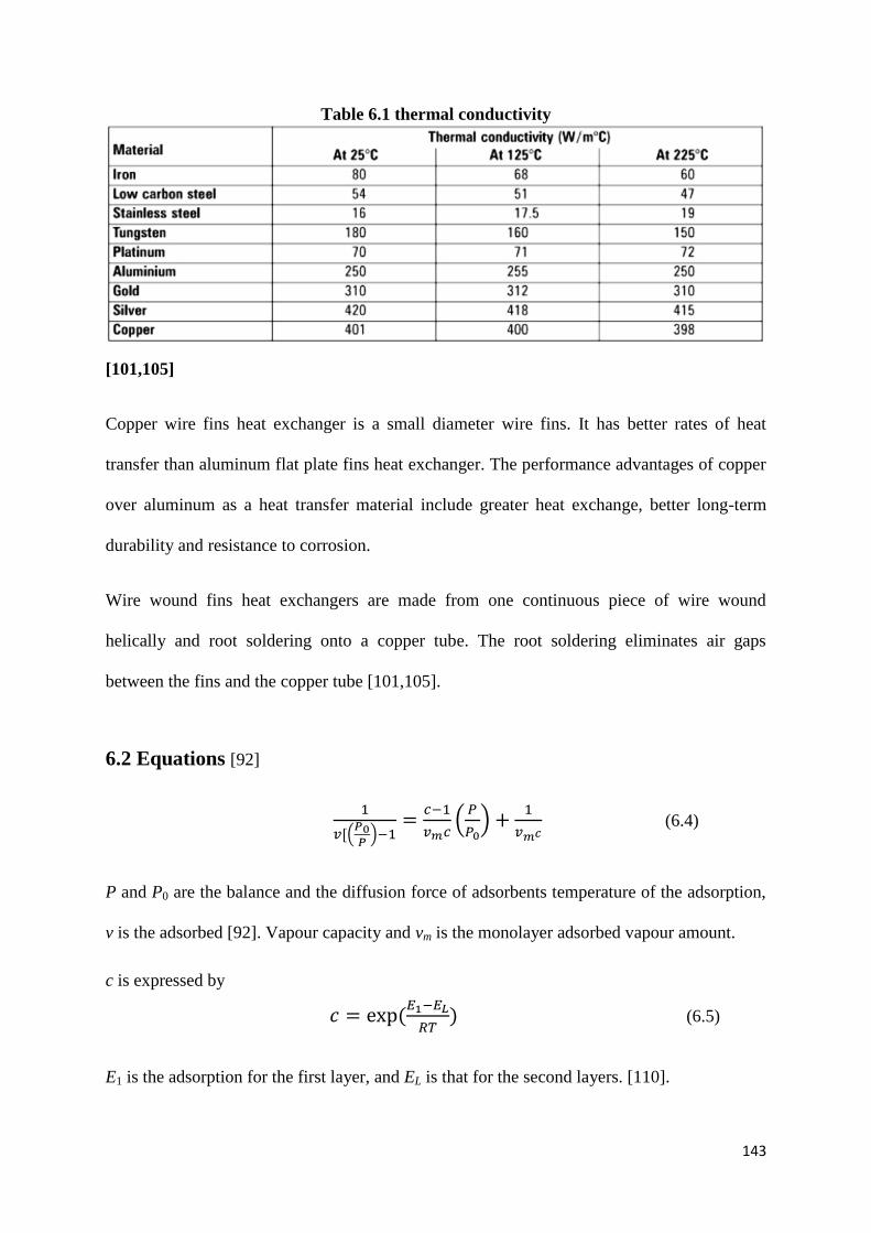
143
Table 6.1 thermal conductivity
[101,105]
Copper wire fins heat exchanger is a small diameter wire fins. It has better rates of heat
transfer than aluminum flat plate fins heat exchanger. The performance advantages of copper
over aluminum as a heat transfer material include greater heat exchange, better long-term
durability and resistance to corrosion.
Wire wound fins heat exchangers are made from one continuous piece of wire wound
helically and root soldering onto a copper tube. The root soldering eliminates air gaps
between the fins and the copper tube [101,105].
6.2 Equations [92]
(
)
(
)
(6.4)
P and P0 are the balance and the diffusion force of adsorbents temperature of the adsorption,
v is the adsorbed [92]. Vapour capacity and vm is the monolayer adsorbed vapour amount.
c is expressed by
(
) (6.5)
E1 is the adsorption for the first layer, and EL is that for the second layers. [110].
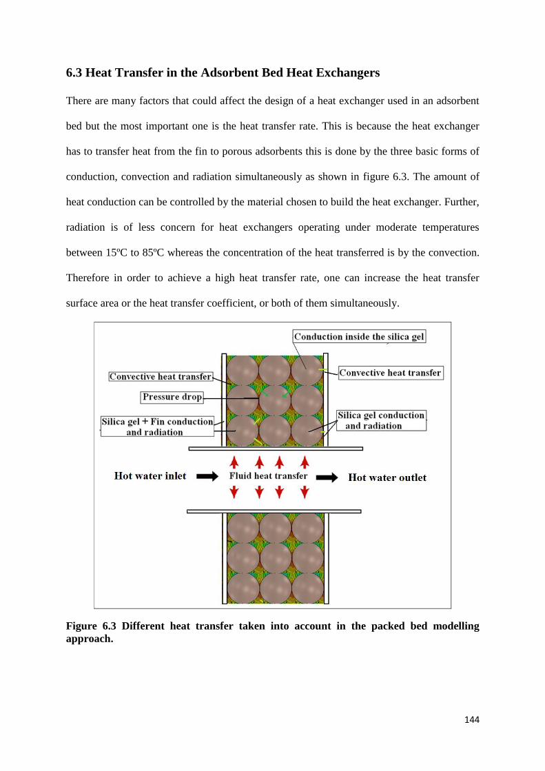
144
6.3 Heat Transfer in the Adsorbent Bed Heat Exchangers
There are many factors that could affect the design of a heat exchanger used in an adsorbent
bed but the most important one is the heat transfer rate. This is because the heat exchanger
has to transfer heat from the fin to porous adsorbents this is done by the three basic forms of
conduction, convection and radiation simultaneously as shown in figure 6.3. The amount of
heat conduction can be controlled by the material chosen to build the heat exchanger. Further,
radiation is of less concern for heat exchangers operating under moderate temperatures
between 15ºC to 85ºC whereas the concentration of the heat transferred is by the convection.
Therefore in order to achieve a high heat transfer rate, one can increase the heat transfer
surface area or the heat transfer coefficient, or both of them simultaneously.
Figure 6.3 Different heat transfer taken into account in the packed bed modelling
approach.
145
6.3.1 The thermal heat transfer of packed beds
Modelling the thermal heat transfer in a porous adsorbent bed includes two main studies (i)
conduction between porous adsorbents and (ii) heat transfer through adsorbed water vapour
and between porous adsorbent. The geometry of a common joint is shown in Figure 6.3
where spherical porous adsorbent are placed in contact. The gap between the contacting
bodies is filled with a water vapour heat is transferred from one sphere adsorbent to another.
The heat transfer through a porous adsorbent bed can be affected by various variables. The
type of porous adsorbent, the packing size, the packing ratio, the inlet water and vapour
temperature, the velocity of the vapour fluid, also the type of refrigerant fluid used in the
evaporator. These various variables will have an significant effect on the heat transfer
phenomenon occurring in the porous adsorbent bed. [1-3].
Another area of particular difficulty in the modelling of heat transfer in a porous adsorbent
bed is the heat transfer near the heat exchanger fins wall. Experimental data used in CFD
simulation modelling are taken from thermocouples fixed to the surface of the heat exchanger
fins. However, due to physical limitations the thermocouples near to the fins it can sometime
be difficult to obtain accurate experimental recordings because of the adsorbent packing near
the fins wall.
6.3.2 Near- Heat Exchanger Fins Wall Small Section Geometries
As mentioned before, computational fluid dynamics modelling is constrained by the available
computational power and the required accuracy. In all modelling cases an appropriate balance
between the two has to be found. For more accurate modelling a more detailed computational
model has to be used, which increases the strain on the simulations. To be able to get more
detailed views of certain areas in the simulation model, or to be able to simulate a specific
section quicker, geometry can be created of a segment of the overall simulation model.
146
Since the major concern in this study is to find the performance of heat transfer from the heat
exchanger fins to the porous adsorbent granules for two different types of heat exchangers,
i.e., copper wire woven fins and aluminium flat plate, segment geometry can be used to
generate simulation results more quickly, due to its limited size. One segment of fins with
porous adsorbent spheres was simulated in order to predict the heat transfer from fin to
porous adsorbents granules. Three dimensional model of a fins and silica gel adsorbent
model can predict the distribution of the thermal heat transfer between fins and porous silica
gel during heating desorption heat phases.
6.4 Heat Transfer Equations
The heat transfer equation is given as
(
)
(
)
(
) (6.6)
The initial condition is
(6.7)
and the boundary conditions are as follows: on the x, y and z symmetries,
(6.8)
on the surfaces of silica gel
(6.9)
where qr is heat loss by radiation on the surface of the fins of the heat exchanger which is
calculated based on the Stefan–Boltzmann law:
(
) (6.10)
147
The water vapour rate sv is,
(6.11)
where fv is the water vapour generation rate for the control volume.
The latent heat of vaporisation of water hfg which can be calculated by the following formula
[101,130].
( ) (6.12)
The Fick’s second law of diffusion can be used to describe mass transfer phenomenon
(
) (6.13)
For mass transfer through the silica gel porous medium, Eq. (6.10) can be rewritten as
(
)
(
) (6.14)
Since concentration is proportional to the partial pressure, when considering water vapour
through a porous medium, concentration can be normally expressed as the equilibrium
relationship in terms of partial pressure [89-110]. Noting that for an ideal gas the
concentration units can be converted to partial pressure units as follows:
(7.15)
Then the inner mass transfer rate is
(
) (6.16)
The mass transfer happens in the area within the adsorbent bed where water vapour is
actually being adsorbed on the silica gel. The mass transfer moves from the input end toward
148
the output end of the adsorbent bed during operation. That is, as the silica gel near the input
becomes saturated with water vapour, the vapour moves toward the output end of the bed
where the silica gel is not yet saturated.
(6.17)
And the boundary conditions are as follows: on the x, y and z symmetries,
(6.18)
on the surfaces,
(6.19)
The vapour transport within the silica gel surface can be treated as vapour movement through
the porous medium [4], which can be expressed as a transfer of vapour in the pores with inner
vapour generation rate.
(
(
)
(
)
(
)) (6.20)
where kv is the mass transfer coefficient of vapour in the vapour-filled pores, which is given
by
(6.21)
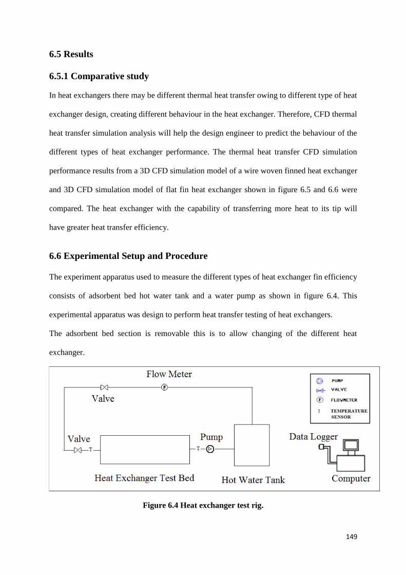
149
6.5 Results
6.5.1 Comparative study
In heat exchangers there may be different thermal heat transfer owing to different type of heat
exchanger design, creating different behaviour in the heat exchanger. Therefore, CFD thermal
heat transfer simulation analysis will help the design engineer to predict the behaviour of the
different types of heat exchanger performance. The thermal heat transfer CFD simulation
performance results from a 3D CFD simulation model of a wire woven finned heat exchanger
and 3D CFD simulation model of flat fin heat exchanger shown in figure 6.5 and 6.6 were
compared. The heat exchanger with the capability of transferring more heat to its tip will
have greater heat transfer efficiency.
6.6 Experimental Setup and Procedure
The experiment apparatus used to measure the different types of heat exchanger fin efficiency
consists of adsorbent bed hot water tank and a water pump as shown in figure 6.4. This
experimental apparatus was design to perform heat transfer testing of heat exchangers.
The adsorbent bed section is removable this is to allow changing of the different heat
exchanger.
Figure 6.4 Heat exchanger test rig.
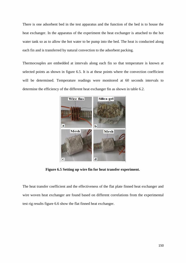
150
There is one adsorbent bed in the test apparatus and the function of the bed is to house the
heat exchanger. In the apparatus of the experiment the heat exchanger is attached to the hot
water tank so as to allow the hot water to be pump into the bed. The heat is conducted along
each fin and is transferred by natural convection to the adsorbent packing.
Thermocouples are embedded at intervals along each fin so that temperature is known at
selected points as shown in figure 6.5. It is at these points where the convection coefficient
will be determined. Temperature readings were monitored at 60 seconds intervals to
determine the efficiency of the different heat exchanger fin as shown in table 6.2.
Figure 6.5 Setting up wire fin for heat transfer experiment.
The heat transfer coefficient and the effectiveness of the flat plate finned heat exchanger and
wire woven heat exchanger are found based on different correlations from the experimental
test rig results figure 6.6 show the flat finned heat exchanger.
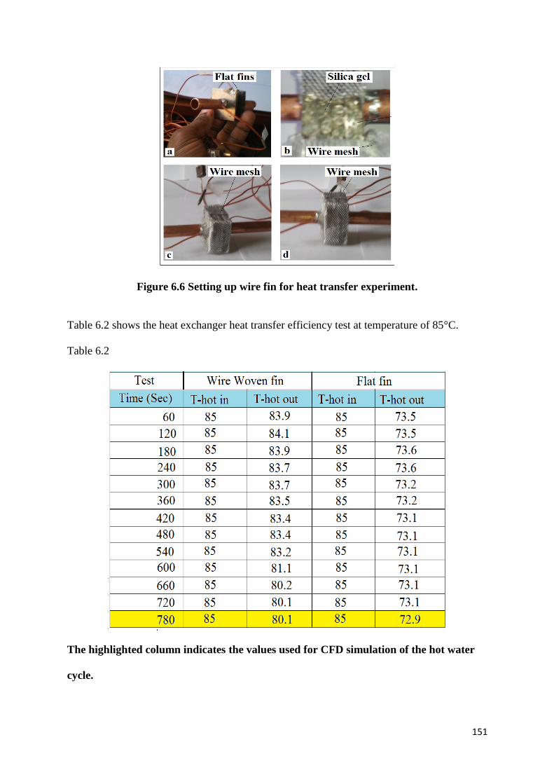
151
Figure 6.6 Setting up wire fin for heat transfer experiment.
Table 6.2 shows the heat exchanger heat transfer efficiency test at temperature of 85°C.
Table 6.2
The highlighted column indicates the values used for CFD simulation of the hot water
cycle.
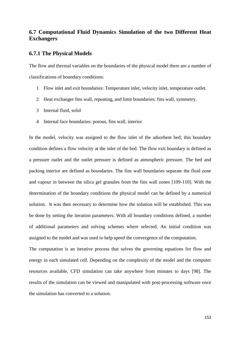
152
6.7 Computational Fluid Dynamics Simulation of the two Different Heat
Exchangers
6.7.1 The Physical Models
The flow and thermal variables on the boundaries of the physical model there are a number of
classifications of boundary conditions:
1 Flow inlet and exit boundaries: Temperature inlet, velocity inlet, temperature outlet.
2 Heat exchanger fins wall, repeating, and limit boundaries: fins wall, symmetry.
3 Internal fluid, solid
4 Internal face boundaries: porous, fins wall, interior
In the model, velocity was assigned to the flow inlet of the adsorbent bed; this boundary
condition defines a flow velocity at the inlet of the bed. The flow exit boundary is defined as
a pressure outlet and the outlet pressure is defined as atmospheric pressure. The bed and
packing interior are defined as boundaries. The fins wall boundaries separate the fluid zone
and vapour in between the silica gel granules from the fins wall zones [109-110]. With the
determination of the boundary conditions the physical model can be defined by a numerical
solution. It was then necessary to determine how the solution will be established. This was
be done by setting the iteration parameters. With all boundary conditions defined, a number
of additional parameters and solving schemes where selected. An initial condition was
assigned to the model and was used to help speed the convergence of the computation.
The computation is an iterative process that solves the governing equations for flow and
energy in each simulated cell. Depending on the complexity of the model and the computer
resources available, CFD simulation can take anywhere from minutes to days [98]. The
results of the simulation can be viewed and manipulated with post-processing software once
the simulation has converted to a solution.
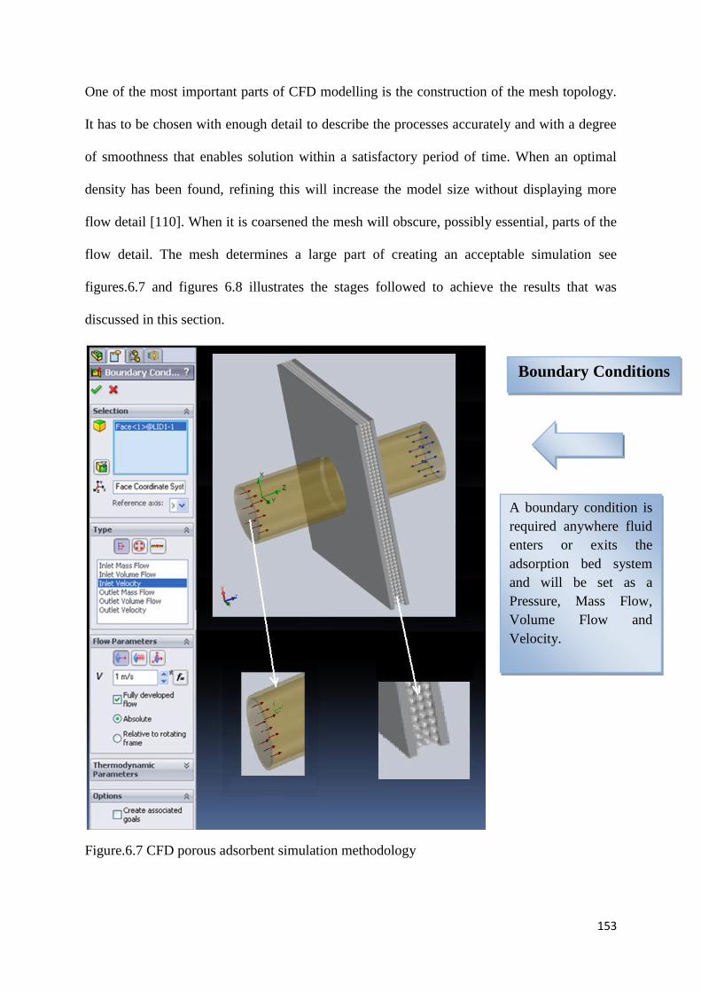
153
One of the most important parts of CFD modelling is the construction of the mesh topology.
It has to be chosen with enough detail to describe the processes accurately and with a degree
of smoothness that enables solution within a satisfactory period of time. When an optimal
density has been found, refining this will increase the model size without displaying more
flow detail [110]. When it is coarsened the mesh will obscure, possibly essential, parts of the
flow detail. The mesh determines a large part of creating an acceptable simulation see
figures.6.7 and figures 6.8 illustrates the stages followed to achieve the results that was
discussed in this section.
Figure.6.7 CFD porous adsorbent simulation methodology
Boundary Conditions
A boundary condition is
required anywhere fluid
enters or exits the
adsorption bed system
and will be set as a
Pressure, Mass Flow,
Volume Flow and
Velocity.
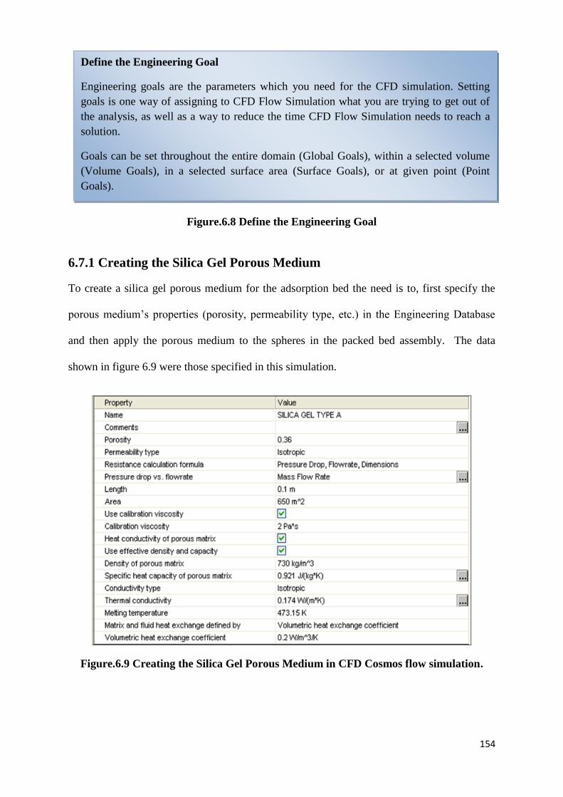
154
Figure.6. 9 Define the Engineering Goal
Figure.6.8 Define the Engineering Goal
6.7.1 Creating the Silica Gel Porous Medium
To create a silica gel porous medium for the adsorption bed the need is to, first specify the
porous medium’s properties (porosity, permeability type, etc.) in the Engineering Database
and then apply the porous medium to the spheres in the packed bed assembly. The data
shown in figure 6.9 were those specified in this simulation.
Figure.6.9 Creating the Silica Gel Porous Medium in CFD Cosmos flow simulation.
Define the Engineering Goal
Engineering goals are the parameters which you need for the CFD simulation. Setting
goals is one way of assigning to CFD Flow Simulation what you are trying to get out of
the analysis, as well as a way to reduce the time CFD Flow Simulation needs to reach a
solution.
Goals can be set throughout the entire domain (Global Goals), within a selected volume
(Volume Goals), in a selected surface area (Surface Goals), or at given point (Point
Goals).
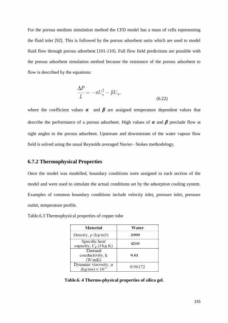
155
For the porous medium simulation method the CFD model has a mass of cells representing
the fluid inlet [92]. This is followed by the porous adsorbent units which are used to model
fluid flow through porous adsorbent [101-110]. Full flow field predictions are possible with
the porous adsorbent simulation method because the resistance of the porous adsorbent to
flow is described by the equations:
(6.22)
where the coefficient values α and β are assigned temperature dependent values that
describe the performance of a porous adsorbent. High values of α and β preclude flow at
right angles to the porous adsorbent. Upstream and downstream of the water vapour flow
field is solved using the usual Reynolds averaged Navier– Stokes methodology.
6.7.2 Thermophysical Properties
Once the model was modelled, boundary conditions were assigned to each section of the
model and were used to simulate the actual conditions set by the adsorption cooling system.
Examples of common boundary conditions include velocity inlet, pressure inlet, pressure
outlet, temperature profile.
Table.6.3 Thermophysical properties of copper tube
Table.6. 4 Thermo-physical properties of silica gel.
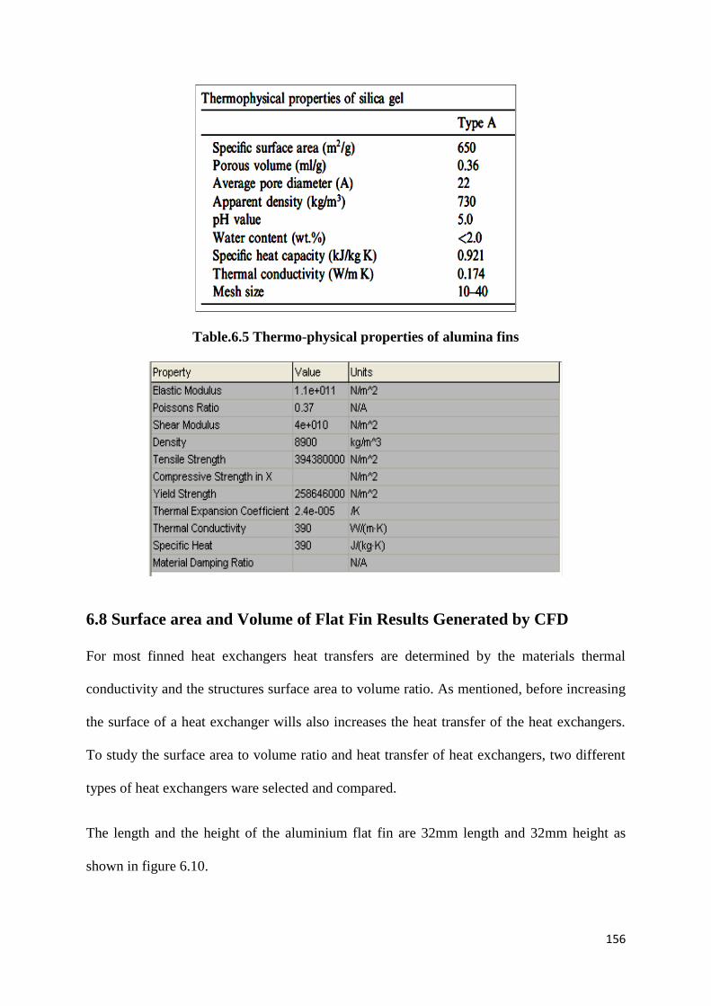
156
Table.6.5 Thermo-physical properties of alumina fins
6.8 Surface area and Volume of Flat Fin Results Generated by CFD
For most finned heat exchangers heat transfers are determined by the materials thermal
conductivity and the structures surface area to volume ratio. As mentioned, before increasing
the surface of a heat exchanger wills also increases the heat transfer of the heat exchangers.
To study the surface area to volume ratio and heat transfer of heat exchangers, two different
types of heat exchangers ware selected and compared.
The length and the height of the aluminium flat fin are 32mm length and 32mm height as
shown in figure 6.10.
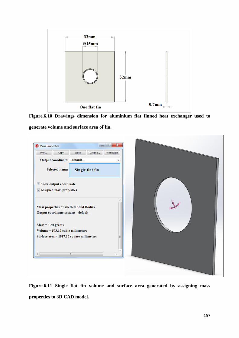
157
Figure.6.10 Drawings dimension for aluminium flat finned heat exchanger used to
generate volume and surface area of fin.
Figure.6.11 Single flat fin volume and surface area generated by assigning mass
properties to 3D CAD model.
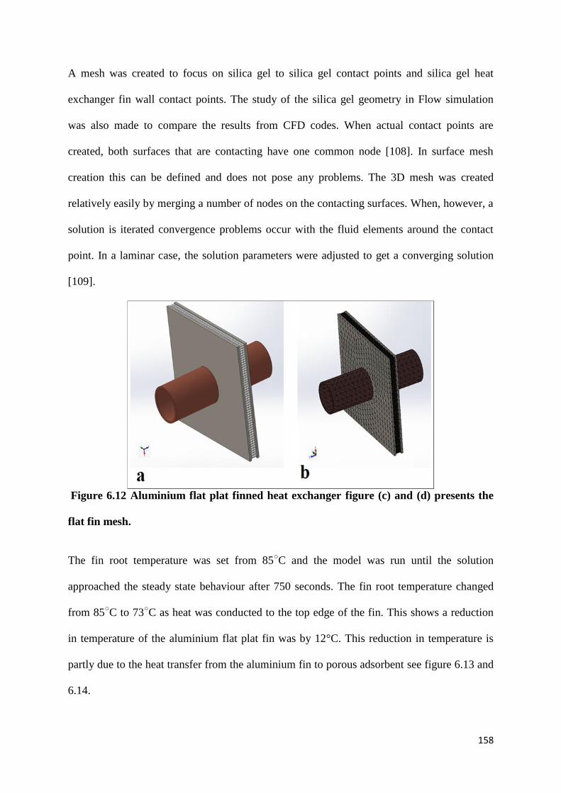
158
A mesh was created to focus on silica gel to silica gel contact points and silica gel heat
exchanger fin wall contact points. The study of the silica gel geometry in Flow simulation
was also made to compare the results from CFD codes. When actual contact points are
created, both surfaces that are contacting have one common node [108]. In surface mesh
creation this can be defined and does not pose any problems. The 3D mesh was created
relatively easily by merging a number of nodes on the contacting surfaces. When, however, a
solution is iterated convergence problems occur with the fluid elements around the contact
point. In a laminar case, the solution parameters were adjusted to get a converging solution
[109].
Figure 6.12 Aluminium flat plat finned heat exchanger figure (c) and (d) presents the
flat fin mesh.
The fin root temperature was set from 85○C and the model was run until the solution
approached the steady state behaviour after 750 seconds. The fin root temperature changed
from 85○C to 73
○C as heat was conducted to the top edge of the fin. This shows a reduction
in temperature of the aluminium flat plat fin was by 12°C. This reduction in temperature is
partly due to the heat transfer from the aluminium fin to porous adsorbent see figure 6.13 and
6.14.
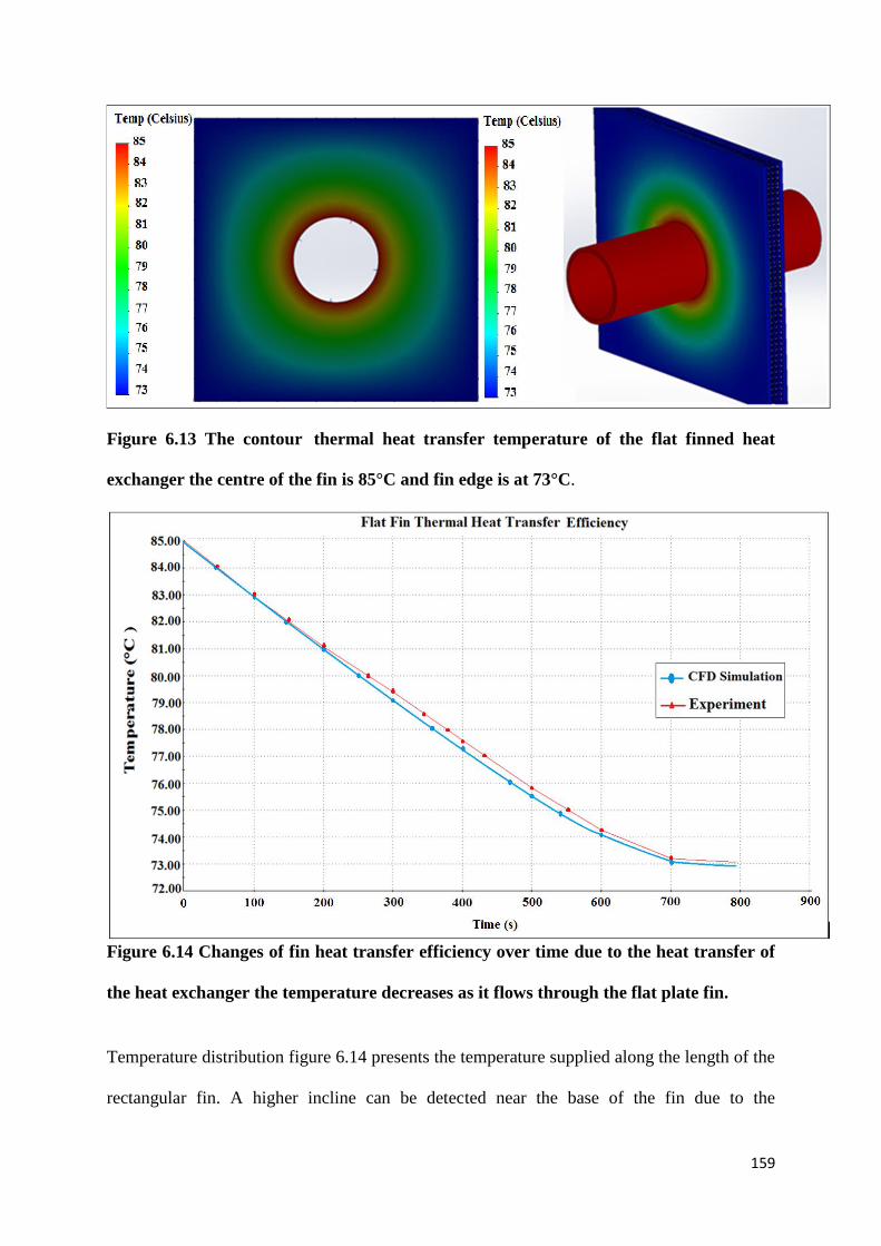
159
Figure 6.13 The contour thermal heat transfer temperature of the flat finned heat
exchanger the centre of the fin is 85°C and fin edge is at 73°C.
Figure 6.14 Changes of fin heat transfer efficiency over time due to the heat transfer of
the heat exchanger the temperature decreases as it flows through the flat plate fin.
Temperature distribution figure 6.14 presents the temperature supplied along the length of the
rectangular fin. A higher incline can be detected near the base of the fin due to the
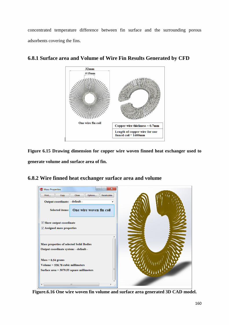
160
concentrated temperature difference between fin surface and the surrounding porous
adsorbents covering the fins.
6.8.1 Surface area and Volume of Wire Fin Results Generated by CFD
Figure 6.15 Drawing dimension for copper wire woven finned heat exchanger used to
generate volume and surface area of fin.
6.8.2 Wire finned heat exchanger surface area and volume
Figure.6.16 One wire woven fin volume and surface area generated 3D CAD model.
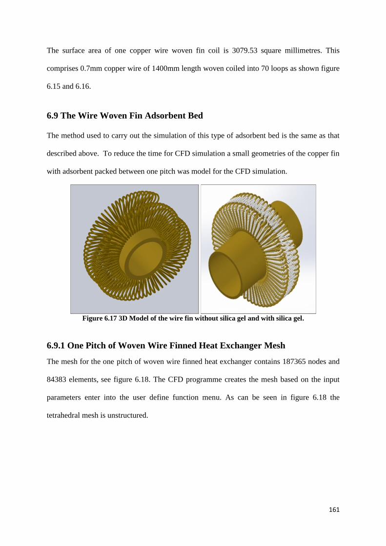
161
The surface area of one copper wire woven fin coil is 3079.53 square millimetres. This
comprises 0.7mm copper wire of 1400mm length woven coiled into 70 loops as shown figure
6.15 and 6.16.
6.9 The Wire Woven Fin Adsorbent Bed
The method used to carry out the simulation of this type of adsorbent bed is the same as that
described above. To reduce the time for CFD simulation a small geometries of the copper fin
with adsorbent packed between one pitch was model for the CFD simulation.
Figure 6.17 3D Model of the wire fin without silica gel and with silica gel.
6.9.1 One Pitch of Woven Wire Finned Heat Exchanger Mesh
The mesh for the one pitch of woven wire finned heat exchanger contains 187365 nodes and
84383 elements, see figure 6.18. The CFD programme creates the mesh based on the input
parameters enter into the user define function menu. As can be seen in figure 6.18 the
tetrahedral mesh is unstructured.
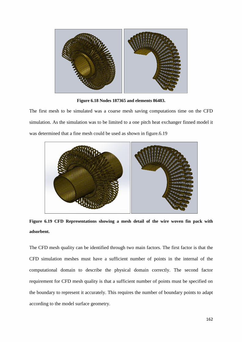
162
Figure 6.18 Nodes 187365 and elements 86483.
The first mesh to be simulated was a coarse mesh saving computations time on the CFD
simulation. As the simulation was to be limited to a one pitch heat exchanger finned model it
was determined that a fine mesh could be used as shown in figure.6.19
Figure 6.19 CFD Representations showing a mesh detail of the wire woven fin pack with
adsorbent.
The CFD mesh quality can be identified through two main factors. The first factor is that the
CFD simulation meshes must have a sufficient number of points in the internal of the
computational domain to describe the physical domain correctly. The second factor
requirement for CFD mesh quality is that a sufficient number of points must be specified on
the boundary to represent it accurately. This requires the number of boundary points to adapt
according to the model surface geometry.
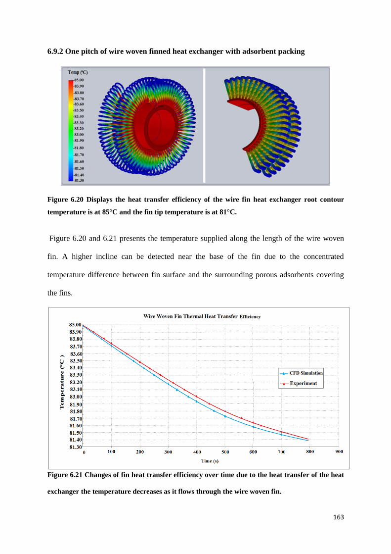
163
6.9.2 One pitch of wire woven finned heat exchanger with adsorbent packing
Figure 6.20 Displays the heat transfer efficiency of the wire fin heat exchanger root contour
temperature is at 85°C and the fin tip temperature is at 81°C.
Figure 6.20 and 6.21 presents the temperature supplied along the length of the wire woven
fin. A higher incline can be detected near the base of the fin due to the concentrated
temperature difference between fin surface and the surrounding porous adsorbents covering
the fins.
Figure 6.21 Changes of fin heat transfer efficiency over time due to the heat transfer of the heat
exchanger the temperature decreases as it flows through the wire woven fin.
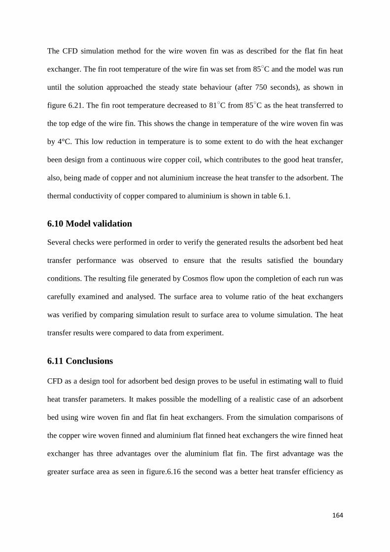
164
The CFD simulation method for the wire woven fin was as described for the flat fin heat
exchanger. The fin root temperature of the wire fin was set from 85○C and the model was run
until the solution approached the steady state behaviour (after 750 seconds), as shown in
figure 6.21. The fin root temperature decreased to 81○C from 85
○C as the heat transferred to
the top edge of the wire fin. This shows the change in temperature of the wire woven fin was
by 4°C. This low reduction in temperature is to some extent to do with the heat exchanger
been design from a continuous wire copper coil, which contributes to the good heat transfer,
also, being made of copper and not aluminium increase the heat transfer to the adsorbent. The
thermal conductivity of copper compared to aluminium is shown in table 6.1.
6.10 Model validation
Several checks were performed in order to verify the generated results the adsorbent bed heat
transfer performance was observed to ensure that the results satisfied the boundary
conditions. The resulting file generated by Cosmos flow upon the completion of each run was
carefully examined and analysed. The surface area to volume ratio of the heat exchangers
was verified by comparing simulation result to surface area to volume simulation. The heat
transfer results were compared to data from experiment.
6.11 Conclusions
CFD as a design tool for adsorbent bed design proves to be useful in estimating wall to fluid
heat transfer parameters. It makes possible the modelling of a realistic case of an adsorbent
bed using wire woven fin and flat fin heat exchangers. From the simulation comparisons of
the copper wire woven finned and aluminium flat finned heat exchangers the wire finned heat
exchanger has three advantages over the aluminium flat fin. The first advantage was the
greater surface area as seen in figure.6.16 the second was a better heat transfer efficiency as
165
seen in figure 6.21 and the third advantage was the smaller volume of the heat exchanger as
showed in figure.6.16.
It was observed from CFD simulation carried out on heat transfer on contact points between
fin and porous adsorbents that the contact points between the adsorbent and heat exchanger
had a significant effect to heat transfer. A poor heat transfer flow distribution can result in a
lower heat transfer rate. Therefore, the optimisation of flow distribution is an essential step in
heat exchanger design optimisation. CFD methods have demonstrated to have great potential
in predicting the performance of both existing and newly developed adsorbent beds designs.
166
CHAPTER 7
SCALING UP THE EXPERIMENTAL INVESTIGATION OF A
WIRE WOVEN HEAT EXCHANGER ADSORPTION BED
PACK WITH SILICA GEL
Abstract
In the previous chapter a CFD comparison study was carried out on a copper wire woven
finned and aluminum flat heat exchanger. The copper wire finned heat exchanger was
considered to have good heat transfer performance compared to the aluminum flat fin.
This chapter describer the experimental work performed on the scaled up adsorption cooling
test rig. It begins with the introduction of the test rig design, its constituting components and
data acquisition system. Performance curves of system components such as the evaporator,
condenser and adsorbent beds are discussed. This chapter also outlines the system behavior
under different operating conditions and a full system CFD simulation.
7.1. Introduction
This chapter prepares the foundation for chapter number 8 which deals with the modelling of
two wires finned adsorbent beds adsorption cooling system. It gives an insight into the
working of the wire woven heat exchanger adsorption cooling system. Procedure of
installation of a test rig equipped with data logging system is given along with the calibration
of sensors. Subsequently the method followed in conducting tests on a new configuration of
adsorption cooling system. The purpose of the testing of the system is to ascertain systems
viability and interaction of individual components. The tests also are carried out to obtain
system parameter for use in the CFD simulation. Several performance curves are produced
for such system components as adsorbent bed evaporator and condenser.
167
7.2 Experimental Set-Up
The adsorption test rig consists of a condenser, evaporator and adsorbent bed. The adsorbent
bed contains a heat exchanger consisting of one silica gel filled copper wire woven fins and
tube. The wire fins contains 0.5 kg of silica gel in total. A heating and cooling water tanks
are used to provide the adsorption bed, condenser and evaporator with water at the desired
temperatures. During the desorption stage of the cycle the adsorption bed is heated to
temperature (80°C) while the condenser is kept at 25°C [82-91]. During the adsorption stage
of the cycle the adsorption bed is cooled down to 25°C and the evaporator to 15°C [90, 91].
Valves with a timer are used to control the heating and cooling water between the cycles of
operation of the adsorbent bed, evaporator and condenser [91].
7.2.1 Components
The experimental test rig set up for adsorption cooling system measurements consisted of the
following components:
1. One adsorbent beds
2. Evaporator
3. Condenser
4. Three water tanks one hot water tank, one cooling water tank and one chilled water
tank
5. Vacuum pump
6. Manually switchable valves, solenoid valves and one diaphragm valve
7. Sensors: Flow meters, pressure transducer and type K thermocouple
8. Measuring: data logger (multiplexes with digital converter) transferring data to a
personal computer
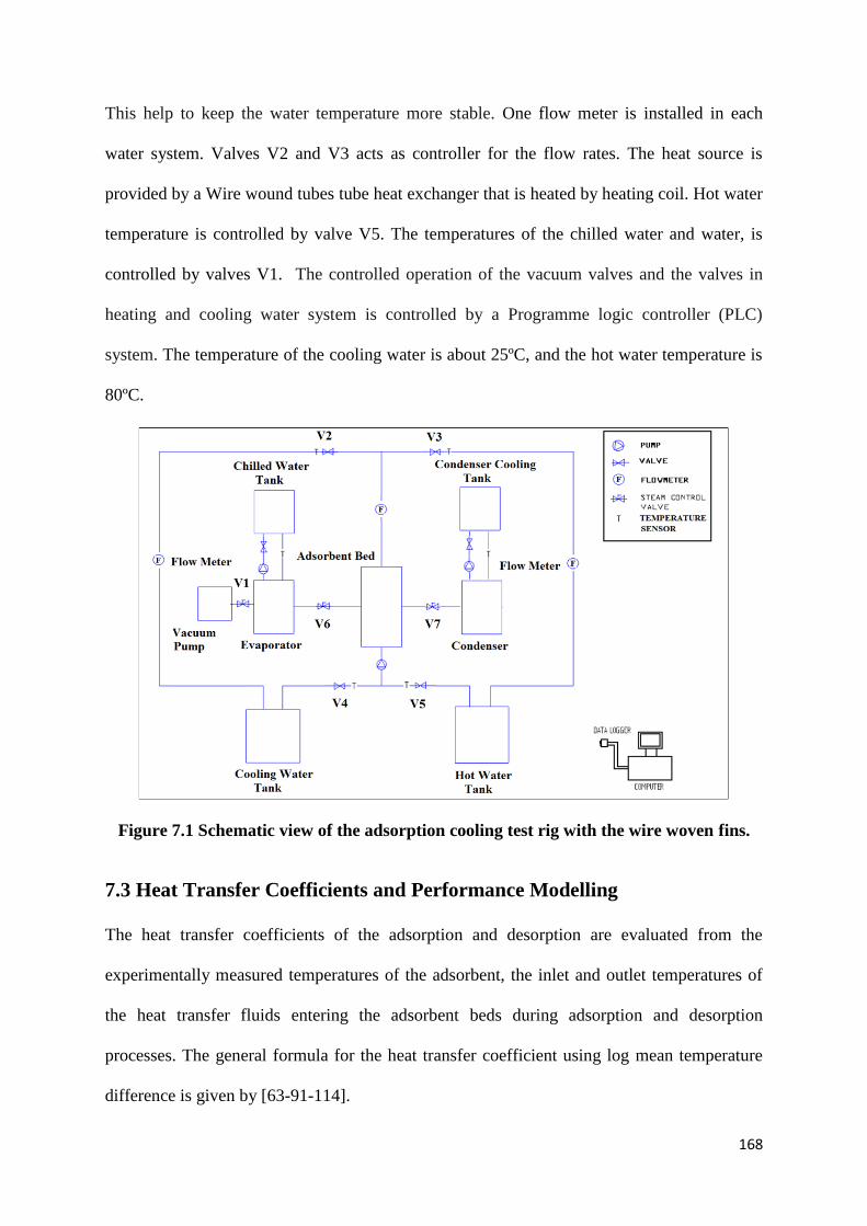
168
This help to keep the water temperature more stable. One flow meter is installed in each
water system. Valves V2 and V3 acts as controller for the flow rates. The heat source is
provided by a Wire wound tubes tube heat exchanger that is heated by heating coil. Hot water
temperature is controlled by valve V5. The temperatures of the chilled water and water, is
controlled by valves V1. The controlled operation of the vacuum valves and the valves in
heating and cooling water system is controlled by a Programme logic controller (PLC)
system. The temperature of the cooling water is about 25ºC, and the hot water temperature is
80ºC.
Figure 7.1 Schematic view of the adsorption cooling test rig with the wire woven fins.
7.3 Heat Transfer Coefficients and Performance Modelling
The heat transfer coefficients of the adsorption and desorption are evaluated from the
experimentally measured temperatures of the adsorbent, the inlet and outlet temperatures of
the heat transfer fluids entering the adsorbent beds during adsorption and desorption
processes. The general formula for the heat transfer coefficient using log mean temperature
difference is given by [63-91-114].
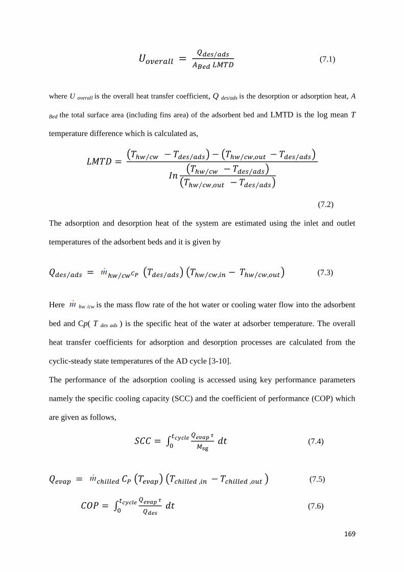
169
⁄
(7.1)
where U overall is the overall heat transfer coefficient, Q des/ads is the desorption or adsorption heat, A
Bed the total surface area (including fins area) of the adsorbent bed and LMTD is the log mean T
temperature difference which is calculated as,
( ⁄ ⁄ ) ( ⁄ ⁄ )
( ⁄ ⁄ )
( ⁄ ⁄ )
(7.2)
The adsorption and desorption heat of the system are estimated using the inlet and outlet
temperatures of the adsorbent beds and it is given by
⁄ ⁄ ( ⁄ ) ( ⁄ ⁄ ) (7.3)
Here hw /cw is the mass flow rate of the hot water or cooling water flow into the adsorbent
bed and Cp( T des ads ) is the specific heat of the water at adsorber temperature. The overall
heat transfer coefficients for adsorption and desorption processes are calculated from the
cyclic-steady state temperatures of the AD cycle [3-10].
The performance of the adsorption cooling is accessed using key performance parameters
namely the specific cooling capacity (SCC) and the coefficient of performance (COP) which
are given as follows,
∫
(7.4)
( ) ( ) (7.5)
∫
(7.6)
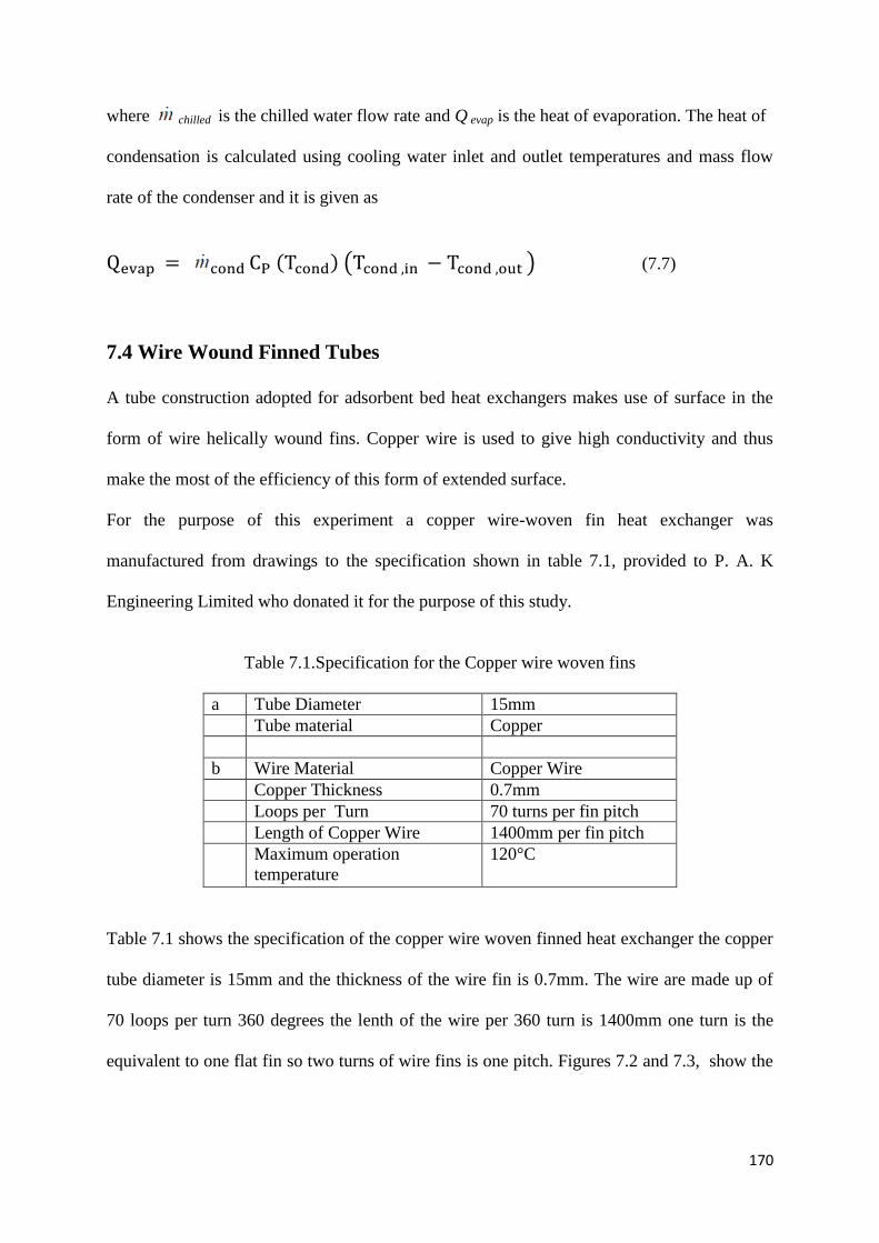
170
where chilled is the chilled water flow rate and Q evap is the heat of evaporation. The heat of
condensation is calculated using cooling water inlet and outlet temperatures and mass flow
rate of the condenser and it is given as
( ) ( ) (7.7)
7.4 Wire Wound Finned Tubes
A tube construction adopted for adsorbent bed heat exchangers makes use of surface in the
form of wire helically wound fins. Copper wire is used to give high conductivity and thus
make the most of the efficiency of this form of extended surface.
For the purpose of this experiment a copper wire-woven fin heat exchanger was
manufactured from drawings to the specification shown in table 7.1, provided to P. A. K
Engineering Limited who donated it for the purpose of this study.
Table 7.1.Specification for the Copper wire woven fins
a Tube Diameter 15mm
Tube material Copper
b Wire Material Copper Wire
Copper Thickness 0.7mm
Loops per Turn 70 turns per fin pitch
Length of Copper Wire 1400mm per fin pitch
Maximum operation
temperature
120°C
Table 7.1 shows the specification of the copper wire woven finned heat exchanger the copper
tube diameter is 15mm and the thickness of the wire fin is 0.7mm. The wire are made up of
70 loops per turn 360 degrees the lenth of the wire per 360 turn is 1400mm one turn is the
equivalent to one flat fin so two turns of wire fins is one pitch. Figures 7.2 and 7.3, show the
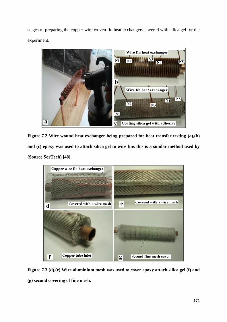
171
stages of preparing the copper wire woven fin heat exchangers covered with silica gel for the
experiment.
Figure.7.2 Wire wound heat exchanger being prepared for heat transfer testing (a),(b)
and (c) epoxy was used to attach silica gel to wire fins this is a similar method used by
(Source SorTech) [48].
Figure 7.3 (d),(e) Wire aluminium mesh was used to cover epoxy attach silica gel (f) and
(g) second covering of fine mesh.
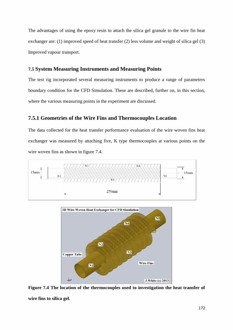
172
The advantages of using the epoxy resin to attach the silica gel granule to the wire fin heat
exchanger are: (1) improved speed of heat transfer (2) less volume and weight of silica gel (3)
Improved vapour transport.
7.5 System Measuring Instruments and Measuring Points
The test rig incorporated several measuring instruments to produce a range of parameters
boundary condition for the CFD Simulation. These are described, further on, in this section,
where the various measuring points in the experiment are discussed.
7.5.1 Geometries of the Wire Fins and Thermocouples Location
The data collected for the heat transfer performance evaluation of the wire woven fins heat
exchanger was measured by attaching five, K type thermocouples at various points on the
wire woven fins as shown in figure 7.4.
Figure 7.4 The location of the thermocouples used to investigation the heat transfer of
wire fins to silica gel.
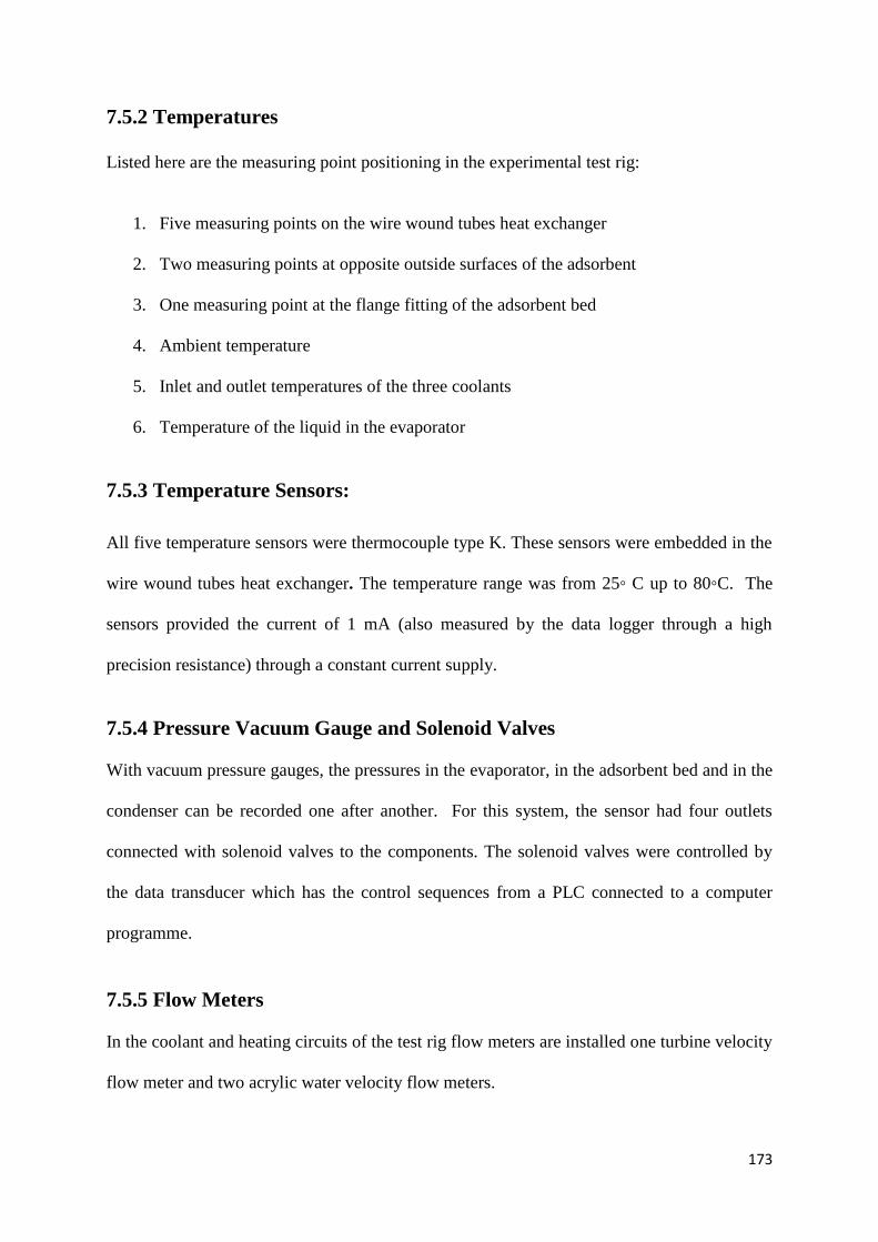
173
7.5.2 Temperatures
Listed here are the measuring point positioning in the experimental test rig:
1. Five measuring points on the wire wound tubes heat exchanger
2. Two measuring points at opposite outside surfaces of the adsorbent
3. One measuring point at the flange fitting of the adsorbent bed
4. Ambient temperature
5. Inlet and outlet temperatures of the three coolants
6. Temperature of the liquid in the evaporator
7.5.3 Temperature Sensors:
All five temperature sensors were thermocouple type K. These sensors were embedded in the
wire wound tubes heat exchanger. The temperature range was from 25◦ C up to 80◦C. The
sensors provided the current of 1 mA (also measured by the data logger through a high
precision resistance) through a constant current supply.
7.5.4 Pressure Vacuum Gauge and Solenoid Valves
With vacuum pressure gauges, the pressures in the evaporator, in the adsorbent bed and in the
condenser can be recorded one after another. For this system, the sensor had four outlets
connected with solenoid valves to the components. The solenoid valves were controlled by
the data transducer which has the control sequences from a PLC connected to a computer
programme.
7.5.5 Flow Meters
In the coolant and heating circuits of the test rig flow meters are installed one turbine velocity
flow meter and two acrylic water velocity flow meters.
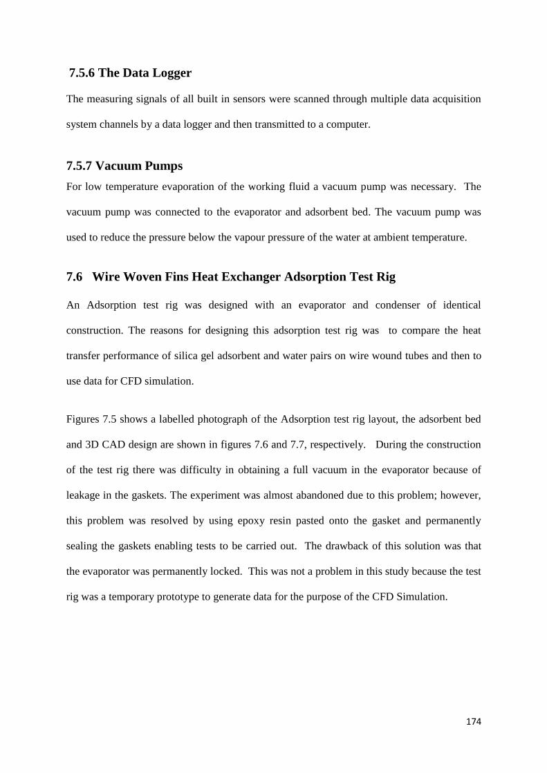
174
7.5.6 The Data Logger
The measuring signals of all built in sensors were scanned through multiple data acquisition
system channels by a data logger and then transmitted to a computer.
7.5.7 Vacuum Pumps
For low temperature evaporation of the working fluid a vacuum pump was necessary. The
vacuum pump was connected to the evaporator and adsorbent bed. The vacuum pump was
used to reduce the pressure below the vapour pressure of the water at ambient temperature.
7.6 Wire Woven Fins Heat Exchanger Adsorption Test Rig
An Adsorption test rig was designed with an evaporator and condenser of identical
construction. The reasons for designing this adsorption test rig was to compare the heat
transfer performance of silica gel adsorbent and water pairs on wire wound tubes and then to
use data for CFD simulation.
Figures 7.5 shows a labelled photograph of the Adsorption test rig layout, the adsorbent bed
and 3D CAD design are shown in figures 7.6 and 7.7, respectively. During the construction
of the test rig there was difficulty in obtaining a full vacuum in the evaporator because of
leakage in the gaskets. The experiment was almost abandoned due to this problem; however,
this problem was resolved by using epoxy resin pasted onto the gasket and permanently
sealing the gaskets enabling tests to be carried out. The drawback of this solution was that
the evaporator was permanently locked. This was not a problem in this study because the test
rig was a temporary prototype to generate data for the purpose of the CFD Simulation.
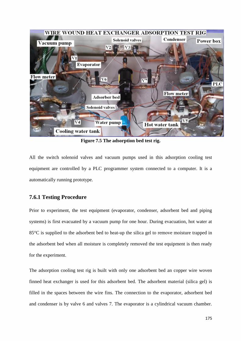
175
Figure 7.5 The adsorption bed test rig.
All the switch solenoid valves and vacuum pumps used in this adsorption cooling test
equipment are controlled by a PLC programmer system connected to a computer. It is a
automatically running prototype.
7.6.1 Testing Procedure
Prior to experiment, the test equipment (evaporator, condenser, adsorbent bed and piping
systems) is first evacuated by a vacuum pump for one hour. During evacuation, hot water at
85°C is supplied to the adsorbent bed to heat-up the silica gel to remove moisture trapped in
the adsorbent bed when all moisture is completely removed the test equipment is then ready
for the experiment.
The adsorption cooling test rig is built with only one adsorbent bed an copper wire woven
finned heat exchanger is used for this adsorbent bed. The adsorbent material (silica gel) is
filled in the spaces between the wire fins. The connection to the evaporator, adsorbent bed
and condenser is by valve 6 and valves 7. The evaporator is a cylindrical vacuum chamber.
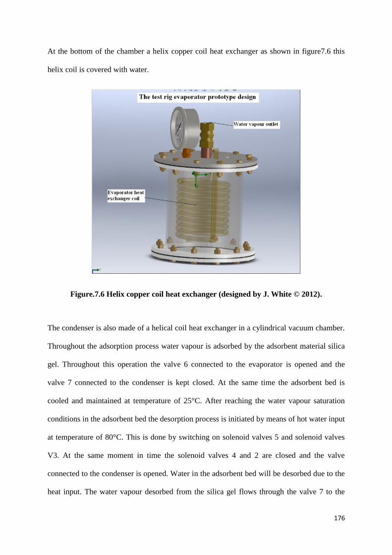
176
At the bottom of the chamber a helix copper coil heat exchanger as shown in figure7.6 this
helix coil is covered with water.
Figure.7.6 Helix copper coil heat exchanger (designed by J. White © 2012).
The condenser is also made of a helical coil heat exchanger in a cylindrical vacuum chamber.
Throughout the adsorption process water vapour is adsorbed by the adsorbent material silica
gel. Throughout this operation the valve 6 connected to the evaporator is opened and the
valve 7 connected to the condenser is kept closed. At the same time the adsorbent bed is
cooled and maintained at temperature of 25°C. After reaching the water vapour saturation
conditions in the adsorbent bed the desorption process is initiated by means of hot water input
at temperature of 80°C. This is done by switching on solenoid valves 5 and solenoid valves
V3. At the same moment in time the solenoid valves 4 and 2 are closed and the valve
connected to the condenser is opened. Water in the adsorbent bed will be desorbed due to the
heat input. The water vapour desorbed from the silica gel flows through the valve 7 to the

177
condenser vacuum chamber. Here the water vapour is condensing on the surface of the
condenser helical coil heat exchanger.
To simulate the experiment under rating conditions, the parameters of the standard operating
condition employed in simulation code are shown in Table 7.2
Table.7.2 Parameters of the standard operating condition employed in simulation code
7.6.2 Considerations and Assumptions
There is no refrigerant vapour or heat losses to the surrounding.
Adsorbent, refrigerant and heat exchanger temperatures are instantaneously the same.
Refrigerant exit from the evaporator at saturated vapour condition.
Refrigerant exit from the condenser at saturated liquid condition.
Flow through the expansion valve is isenthalpic flow.
The isosteric heat of adsorption is assumed constant.
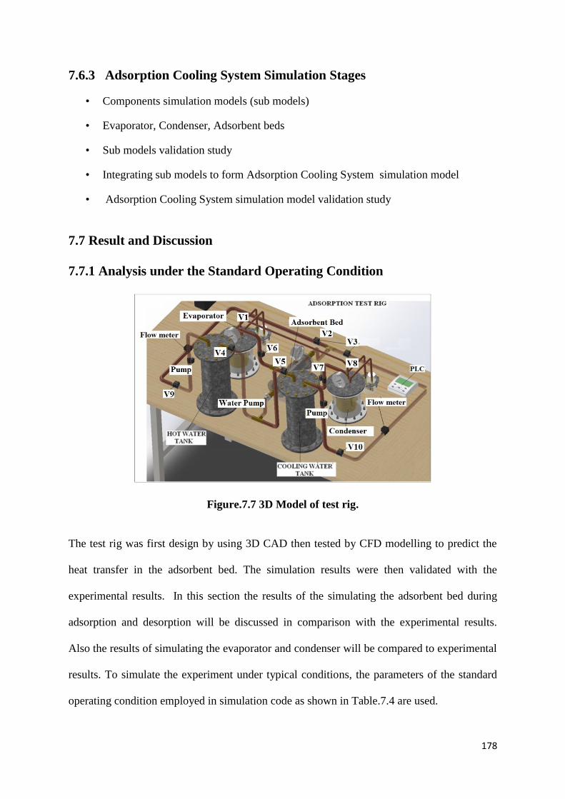
178
7.6.3 Adsorption Cooling System Simulation Stages
• Components simulation models (sub models)
• Evaporator, Condenser, Adsorbent beds
• Sub models validation study
• Integrating sub models to form Adsorption Cooling System simulation model
• Adsorption Cooling System simulation model validation study
7.7 Result and Discussion
7.7.1 Analysis under the Standard Operating Condition
Figure.7.7 3D Model of test rig.
The test rig was first design by using 3D CAD then tested by CFD modelling to predict the
heat transfer in the adsorbent bed. The simulation results were then validated with the
experimental results. In this section the results of the simulating the adsorbent bed during
adsorption and desorption will be discussed in comparison with the experimental results.
Also the results of simulating the evaporator and condenser will be compared to experimental
results. To simulate the experiment under typical conditions, the parameters of the standard
operating condition employed in simulation code as shown in Table.7.4 are used.
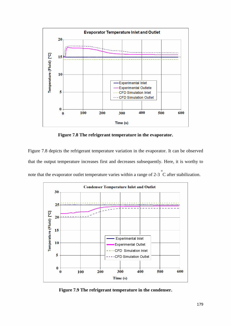
179
Figure 7.8 The refrigerant temperature in the evaporator.
Figure 7.8 depicts the refrigerant temperature variation in the evaporator. It can be observed
that the output temperature increases first and decreases subsequently. Here, it is worthy to
note that the evaporator outlet temperature varies within a range of 2-3 o
C after stabilization.
Figure 7.9 The refrigerant temperature in the condenser.
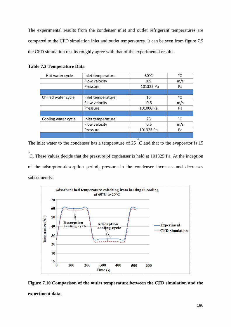
180
The experimental results from the condenser inlet and outlet refrigerant temperatures are
compared to the CFD simulation inlet and outlet temperatures. It can be seen from figure 7.9
the CFD simulation results roughly agree with that of the experimental results.
Table 7.3 Temperature Data
Hot water cycle Inlet temperature 60°C °C
Flow velocity 0.5 m/s
Pressure 101325 Pa Pa
Chilled water cycle Inlet temperature 15 °C
Flow velocity 0.5 m/s
Pressure 101000 Pa Pa
Cooling water cycle Inlet temperature 25 °C
Flow velocity 0.5 m/s
Pressure 101325 Pa Pa
The inlet water to the condenser has a temperature of 25 o
C and that to the evaporator is 15
o
C. These values decide that the pressure of condenser is held at 101325 Pa. At the inception
of the adsorption-desorption period, pressure in the condenser increases and decreases
subsequently.
Figure 7.10 Comparison of the outlet temperature between the CFD simulation and the
experiment data.
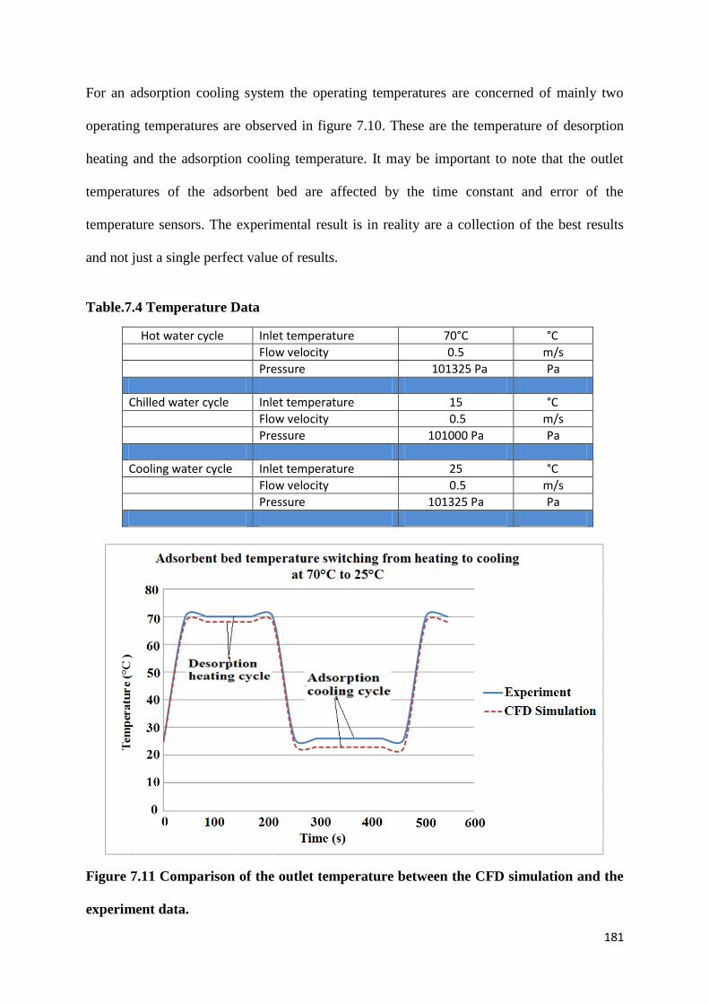
181
For an adsorption cooling system the operating temperatures are concerned of mainly two
operating temperatures are observed in figure 7.10. These are the temperature of desorption
heating and the adsorption cooling temperature. It may be important to note that the outlet
temperatures of the adsorbent bed are affected by the time constant and error of the
temperature sensors. The experimental result is in reality are a collection of the best results
and not just a single perfect value of results.
Table.7.4 Temperature Data
Hot water cycle Inlet temperature 70°C °C
Flow velocity 0.5 m/s
Pressure 101325 Pa Pa
Chilled water cycle Inlet temperature 15 °C
Flow velocity 0.5 m/s
Pressure 101000 Pa Pa
Cooling water cycle Inlet temperature 25 °C
Flow velocity 0.5 m/s
Pressure 101325 Pa Pa
Figure 7.11 Comparison of the outlet temperature between the CFD simulation and the
experiment data.
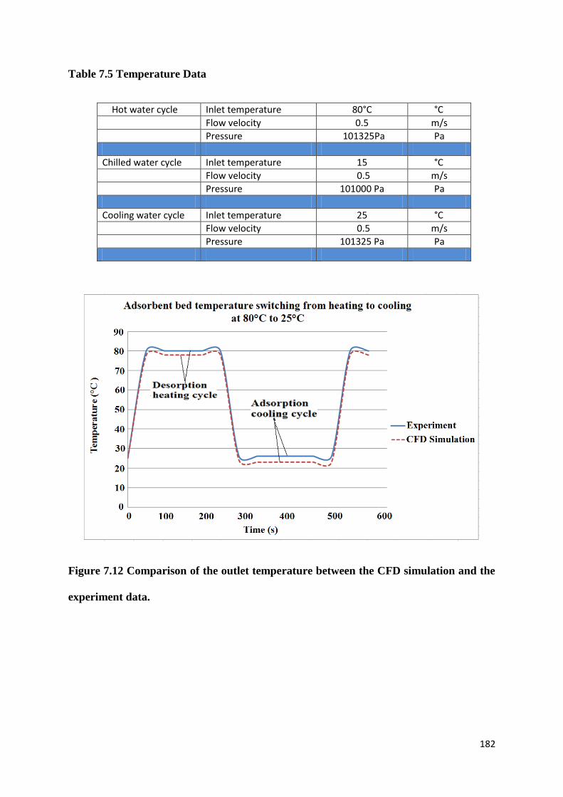
182
Table 7.5 Temperature Data
Hot water cycle Inlet temperature 80°C °C
Flow velocity 0.5 m/s
Pressure 101325Pa Pa
Chilled water cycle Inlet temperature 15 °C
Flow velocity 0.5 m/s
Pressure 101000 Pa Pa
Cooling water cycle Inlet temperature 25 °C
Flow velocity 0.5 m/s
Pressure 101325 Pa Pa
Figure 7.12 Comparison of the outlet temperature between the CFD simulation and the
experiment data.
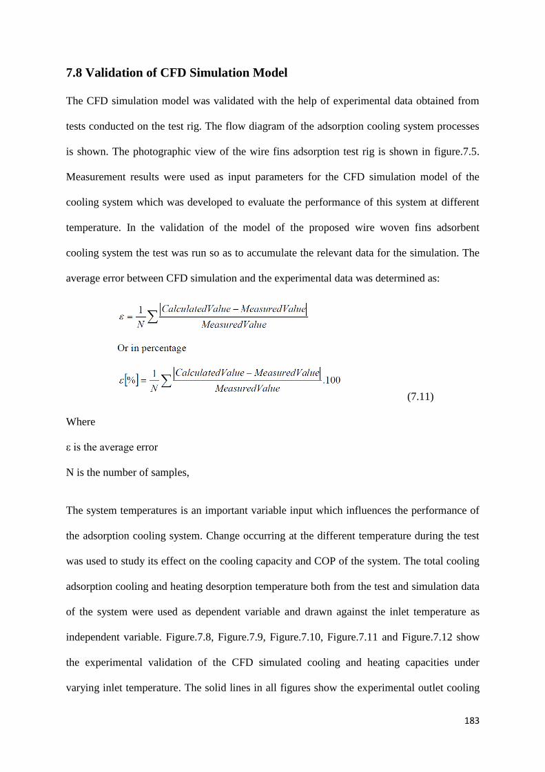
183
7.8 Validation of CFD Simulation Model
The CFD simulation model was validated with the help of experimental data obtained from
tests conducted on the test rig. The flow diagram of the adsorption cooling system processes
is shown. The photographic view of the wire fins adsorption test rig is shown in figure.7.5.
Measurement results were used as input parameters for the CFD simulation model of the
cooling system which was developed to evaluate the performance of this system at different
temperature. In the validation of the model of the proposed wire woven fins adsorbent
cooling system the test was run so as to accumulate the relevant data for the simulation. The
average error between CFD simulation and the experimental data was determined as:
(7.11)
Where
ε is the average error
N is the number of samples,
The system temperatures is an important variable input which influences the performance of
the adsorption cooling system. Change occurring at the different temperature during the test
was used to study its effect on the cooling capacity and COP of the system. The total cooling
adsorption cooling and heating desorption temperature both from the test and simulation data
of the system were used as dependent variable and drawn against the inlet temperature as
independent variable. Figure.7.8, Figure.7.9, Figure.7.10, Figure.7.11 and Figure.7.12 show
the experimental validation of the CFD simulated cooling and heating capacities under
varying inlet temperature. The solid lines in all figures show the experimental outlet cooling
184
and heating temperature variation over time and dots represent the CFD cooling temperature
variation over time. It is clear from the observation of these figures that both simulation and
test results show same trend i.e., the cooling temperature were proportional. An agreement of
validation was observed for most of the data error analysis showed a deviation of 6% and 3.4
% respectively.
7.9 Conclusion
The simulation code has been tested for stability in computation and is able to achieve CFD
simulation of the wire woven fin heat exchanger and the different components of the
adsorption cooling system. The comparison of CFD simulated results and experimental data
proves that the CFD model is reliable tool.
With this simulation tool, the time and cost of designing an adsorption cooling system could
be reduced for the design of a one adsorbent bed system as it provides valuable prediction for
component performances. With minor modification, it can be extended for use on other
configurations of multi-bed system.
185
CHAPTER 8
CONCLUSIONS AND PROSPECT FOR FUTURE WORK
8.1 Introduction
In addition to the conclusions drawn at the end of each chapter, this chapter sums up the
important results and conclusions obtained from the detailed study of earlier works done in
the area of adsorption cooling technologies. Additionally, this chapter also presents the main
findings of present research. This is followed by relevant recommendations for future
research and development.
8.2 Conclusions
The CFD simulation of the adsorption cooling system using copper wire woven finned heat
exchanger packed with silica gel has been successfully simulated. CFD comparison study
was carried out on a copper wire woven finned and aluminum flat finned heat exchanger. The
copper wire woven finned heat exchanger was considered to have better heat transfer
performance compared to the aluminum flat fin. The use of CFD simulation approach to
simulate adsorption cooling system differs from most simulation work reported in the literature
on adsorption cooling systems. The simulation code has been tested for capability of
simulating adsorption system heat transfer. A comparison of simulated results and
experimental data proves that the CFD simulation model is a reliable tool.
Due to the improvement in porous media CFD simulation, the water vapour uptake or off-
take of the adsorbent beds can now be accurately simulated in terms of heat transfer and
porous adsorbent bed design. Using CFD simulation code the time and cost of designing an
adsorption cooling system could be reduced as it provides valuable prediction for component
performances with minor modification.
186
8.3 Suggestions for Further Work
A solution to the need for a configuration with a larger surface area could be to redesign the
adsorbent bed to accommodate a copper wire woven fins heat exchanger. This type of heat
exchanger increases the surface area because of the fine wire configuration. The review of
the literature indicates a lack of work being carried out on this type of heat exchanger in
adsorption cooling systems, leading to the concept design by the researcher of a copper wire
woven finned adsorbent bed and a lab test rig to test the performance of this type of heat
exchanger. Copper wire woven finned heat exchangers are commonly used in oil heating
system. This can be redesigned for adsorbent beds used in adsorption cooling systems and
would solve one of the heat transfer problems of the heat exchanger.
In this study, CFD simulation modelling was used to help design a new copper wire woven
finned and silica gel adsorbent bed. It is expected that the analysis of this will help contribute
towards research and development of adsorption cooling technologies. For this to be
achieved, additional research is needed to redesign a full adsorption cooling system that could
be used, for example, as a cooler display unit. This system could then be tested against a
mechanical vapour system, over a period of time, in order to validate its performance.
In order for this new full adsorption cooling system to have high performance in terms of
coefficient of performance the following should be preferred.
1. A copper wire woven heat exchanger should be chosen rather than aluminium flat
plate fin heat exchanger since copper has higher thermal efficiency than aluminium
and wire fin have a lager surface area than a flat plate fin heat exchanger.
2. The CFD simulation models should be supported with experimental studies of the
prototypes. The modelled cycles should be constructed and analysed to further verify
the results of CFD simulation models.
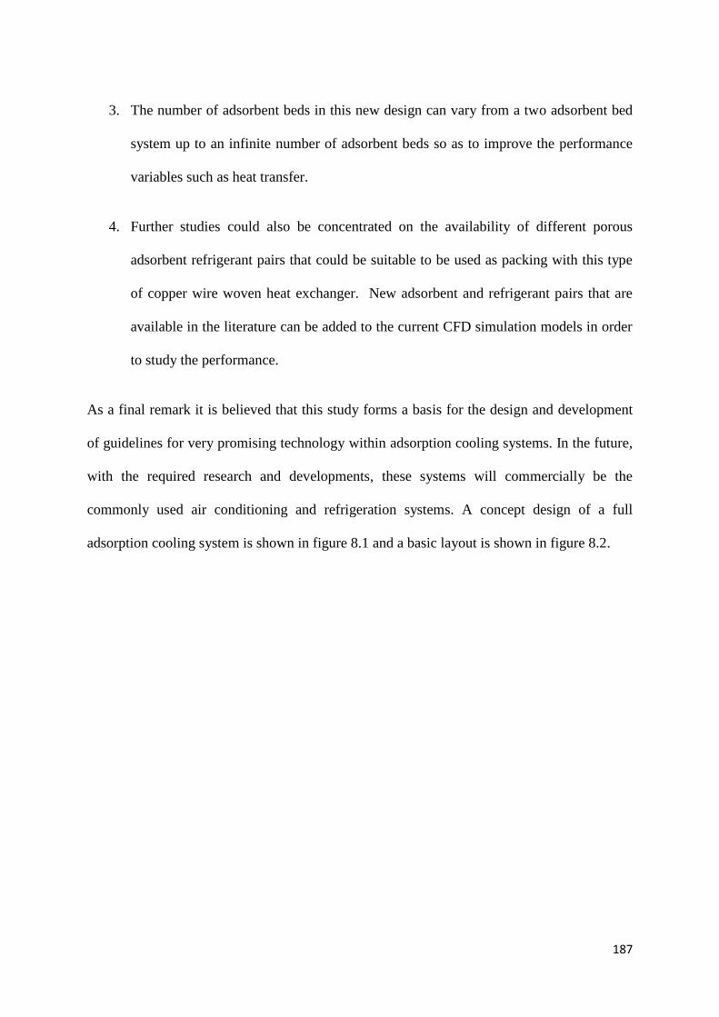
187
3. The number of adsorbent beds in this new design can vary from a two adsorbent bed
system up to an infinite number of adsorbent beds so as to improve the performance
variables such as heat transfer.
4. Further studies could also be concentrated on the availability of different porous
adsorbent refrigerant pairs that could be suitable to be used as packing with this type
of copper wire woven heat exchanger. New adsorbent and refrigerant pairs that are
available in the literature can be added to the current CFD simulation models in order
to study the performance.
As a final remark it is believed that this study forms a basis for the design and development
of guidelines for very promising technology within adsorption cooling systems. In the future,
with the required research and developments, these systems will commercially be the
commonly used air conditioning and refrigeration systems. A concept design of a full
adsorption cooling system is shown in figure 8.1 and a basic layout is shown in figure 8.2.
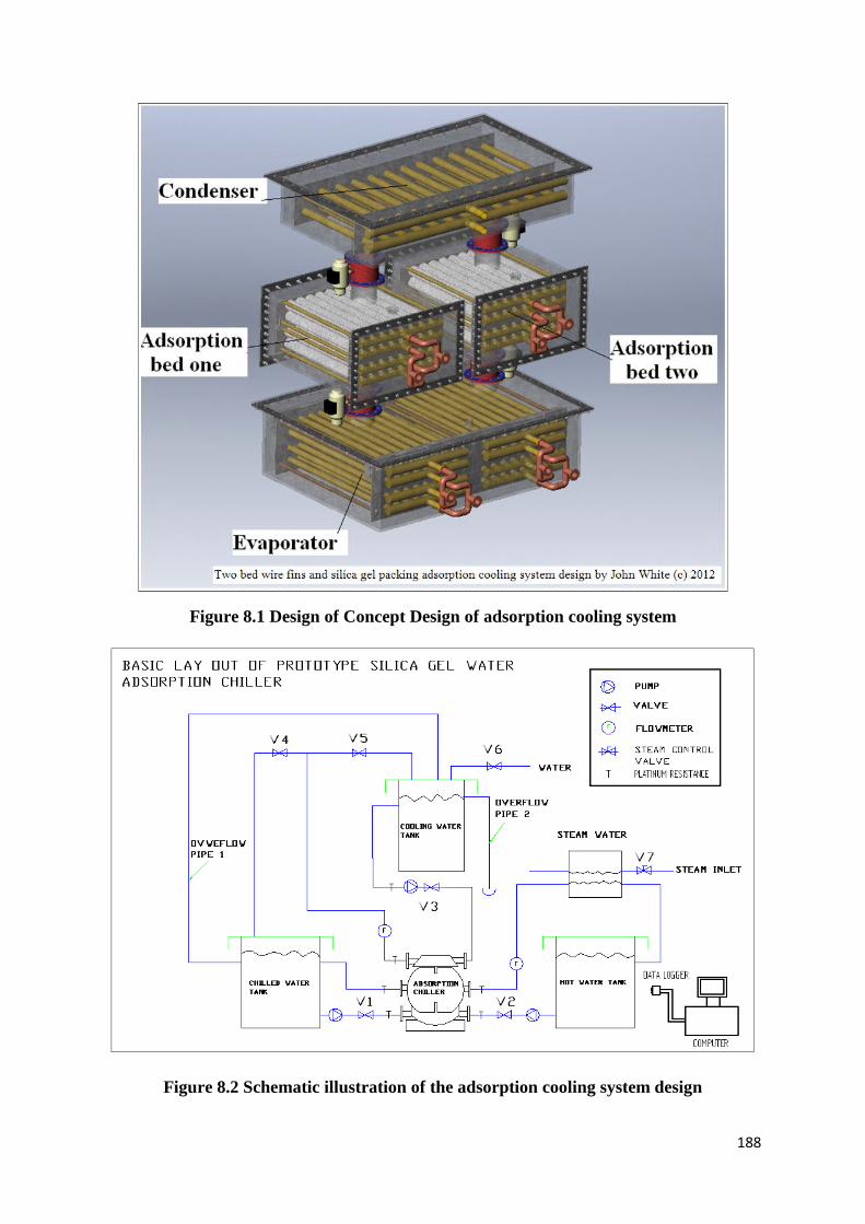
188
Figure 8.1 Design of Concept Design of adsorption cooling system
Figure 8.2 Schematic illustration of the adsorption cooling system design
189
REFERENCES
[1] Augier .F, Laroche .C., Brehon. E. (2008) Application of Computational Fluid
Dynamics to Fixed Bed Adsorption Calculations: University of Science and
Technology, Beijing.
[2] Mueller, G. E. (1992) Radial void draction distributions in randomly packed fixed
bedsof uniformly sized spheres in cylindrical containers in, Powder Technology, Vol
72(3) pp. 269-275.
[3] Rahimi, M. and Mohseni, M. (2008) CFD modelling of the effect of absorbent size
on absorption performance of a packed bed column in Korean Journal of Chemical
Engineering, vol. 25, no. 3, pp. 395–401.
[4] Murakami, S, Kato, S., Ito, K. and Zhu Q. (2003) Modelling and CFD prediction for
diffusion and adsorption within room with various adsorption isotherms. In Indoor Air
13, Supplement 6, pp.20-27.
[5] Critoph, R.E., (1996) Evaluation of alternative refrigerant-adsorbent pairs for
refrigeration cycles. Applied Thermal Engineering,.16: p. 891-900.
[6] Kuipers, J.A.M., Van Swaaij, W.P.M., (1998) In Wei, J., Anderson, J., Bischoff, K.,
Denn, M., Seinfield, J., Stephanopoulos, G., eds.; Advances in Chemical Engineering.
Academic Press, San Diego, p.227.
[7] Ranade,V., (2002) Computational Flow Modeling for Chemical Reactor Engineering.
Academic Press, New York.
[8] Nuntaphan Atipoang, Vithayasai Sanparwat, Vorayos Nat, Vorayos Nattanee and
Kiatsiriroat Tanongkiat. (2010) Use of oscillating heat pipe technique as extended
surface in wire-on-tube heat exchanger for heat transfer enhancement International
Communications in Heat and Mass Transfer Vol. 37, 287–292
[9] Miller, E.B. (1929) The Development of Silica Gel, Refrigerating Engineering in The
American Society of Refrigerating Engineers. 17(4) pp. 103-108.
190
[10] IGT, (1972) Technical feasibility of solid adsorption cooling system, Institute of Gas
Technology, Project HC-4-15, December.
[11] Tchernev, D.I., (1979) Solar Air Conditioning and Refrigeration Systems Utilizing
zeolites. Proceeding of meetings of Commissions E1-E2, Jerusalem, Issued by
International Institute of Refrigeration, pp. 209-215.
[12] Meunier, F. (2002) Sorption Contribution to Climate Change mitigation, in:
Proceedings of the International Sorption Heat Pump Conference, Shanghai.
September 24-27.
[13] Sakoda, A., & Suzuki, M., (1984) Fundamental study on solar powered adsorption
cooling system. Journal of Chemical Engineering, Japan, Vol. 17, No. 1pp.52-57.
[14] Sakoda, A. and Suzuki M (1986) Simultaneous Transport of Heat and Adsorbate in
Closed Type Adsorption Cooling System Utilizing Solar Heat Journal of Solar
Energy Engineering. Vol.108, pp.239-245.
[15] Kluppel, R.P. and Gurgel, J.M.A.M. (1988) Solar Cooled Drinking Fountain. Sunworld,
Vol 12, No 4, pp 113-4.
[16] Cho, S.H. and Kim, J.N., (1992) Modelling of a Silica Gel/Water Adsorption-Cooling
System, Energy, Vol. 17, No.9, pp.829-39.
[17] Watabe, Y. and Yanadori M., (1994).Cooling characteristic of adsorpti refrigeration
apparatus using silica gel-ethanol system. Kagakii Kogakii Ronbunshu, Vol.20, No.4,
pp.589-593.
[18] Saha, B.B., Boelman, E.C., and Kashiwagi, (1995).T. Computational analysis of an
advanced adsorption-refrigeration cycle, Energy, Vol. 20, No 10, pp.983-94
[19] Boelman, E.C., Saha, B.B., and Kashiwagi, T., (1997). Parametric Study of a Silica
Gel-water Adsorption Refrigeration Cycle-the Influence of Thermal Capacitance and
Heat Exchanger UAvalues on Cooling Capacity, Power Density, and COP. ASHRAE
Transactions, Vol 103. No 1, pp.l37-48
191
[20] Alam et.al (2000) Heat exchanger design effect on the system performance of silica gel
water adsorption system International Journal of Heat Mass Transfer. Vol.43. pp.
4419-4431.
[21] Anyanwu E.E., and Ezekwe C.I., (2003) Design, construction and test run of a solid
adsorption solar refrigerator using activated carbon/methanol, as adsorbent/adsorbate
pair, Energy Conversion and Management (44) pp 2879-2892
[22] Tanaka S., Hasegawa T., and Waki T. (1983) On the integrated solar collector-chiller
using the intermittent adsorption cycle. I.S.E.S. Solar World Congress, August 14-19,
Perth.
[23] Wang, R.Z., and Oliveira, R.G., (2005). Adsorption refrigeration An Efficient Way to
Make Good Use of Waste Heat and Solar Energy Proceedings of International
Sorption Heat Pump Conference, Denver, USA.
[24] Anyanwu, E.E, and Ogueke, N.V., (2005) Thermodynamic design procedure for solid
adsorption solar refrigerator, Renewable Energy (30) pp. 81-96.
[25] Chang W.-S, Wang C.-C and Shieh C.-C (2005) Experimental study of a solid
adsorption cooling system using flat-tube heat exchangers as adsorption bed Applied
Thermal Engineering 27 2195–2199.
[26] Jakob, I., and Walter Mittelbach, W., (2008) Development and Investigation of a
Compact silica gel/water adsorption chiller integrated in solar cooling systems, VII
Minsk, International Seminar, “Heat, Pumps, Refrigerators, Power Sources”. Minsk,
Belarus, September 8-11.
[27] Rouquerol. J., et al (1994) Recommendations for the characterization of porous solids
(Technical Report) International Union of Pure and Applied Chemistry, Vol.66, No.8,
pp.1739-1758
[28] Liu, Y., Leong. K.C., (2005) The effect of operating conditions on the performance of
zeolite/water adsorption cooling systems. Technological University Applied Thermal
Engineering, Vol.25 (10) pp. 1403–1418.
192
[29] Menard D., Py X., Mazet N., (2005) Activated carbon monolith of high thermal
conductivity for adsorption processes improvement Part A: Adsorption step, Chemical
Engineering and Processing Vol 44(9) pp. 1029–1038.
[30] Saha, B.B., El-Sharkawy, I.I, Chakraborty, A., Koyama, S. (2007) Study on an
activated carbon fiber–ethanol adsorption chiller. Part II, Performance evaluation.
Internation Journal Refrigeration, Vol.30. (1) pp.96–102.
[31] Huang, J., et al., (2007) Adsorption studies of a water soluble dye, Reactive Red MF-
3B, using sonication-surfactant-modified attapulgite clay. Journal of Hazardous
Materials Vol.143, pp 541–548.
[32] Hai-Jun, C., .et al., (2008) Attapulgite based LiCl composite adsorbents for cooling
and air conditioning applications, Applied Thermal Engineering. Vol. 28 pp. 2187–
2193.
[33] Wang, L.W., (2009). A review on adsorption working pairs for refrigeration,
Renewable and Sustainable Energy. Vol.13 (3) pp.518-534.
[34] Dabrowski, A., (2001) Adsorption-from theory to practice. Advances in Colloid and
Interface Science Vol. 93 pp. 136-224.
[35] Fripiat, J.J., Gatineau, L., Van Damme, H (1986), Multilayer Physical Adsorption on
Fractal Surfaces, Langmuir, Vol.2 (5) pp. 565-567.
[36] Qiu, S., and Zhu. G., (2009) Molecular engineering for synthesizing novel structures of
metal–organic frameworks with multifunctional properties Coordination Chemsistry
Reviews, Vol 253 (23) pp. 2892-2910.
[37] Aranovich, G., and Donohue, M., (1998) Analysis of Adsorption Isotherms: Lattice
Theory Predictions, Classification of Isotherms for Gas–Solid Equilibria, and
Similarities in Gas and Liquid Adsorption Behavior. Journal of Colloid and Interface
Science Vol.200 (2), pp. 273-290.
193
[38] Sangwichien, C., Aranovich, G.L., and Donohue, M.D., (2002) Density functional
theory predictions of adsorption isotherms with hysteresis loops. Colloids and
Surfaces A: Physicochemical and Engineering Aspects, 206, pp. 313–320.
[39] Somorjai, G.A., (1972) Principles of Surface Chemistry, Prentice-Hall, Englewood
Cliffs, N. J.
[40] San J.Y., Wei-Min Lin W.M, (2008) Comparison among three adsorption pairs for
using as the working substances in a multi-bed adsorption heat pump, Applied
Thermal Engineering. Vol 28, Issues 8-9, pp. 801-11-8.
[41] Sing, K.S.W., (2004) Characterization of porous materials: past, present and future,
Colloids and Surfaces A: Physicochemical Engineering Aspects. 241, pp.3-7.
[42] Chua, H.T., Ng, K.C., Chakraborty, A., Nay, M.O. and Othman, M.A., (2002)
Adsorption characteristic of silica gel + water systems, Journal of Chemical and
Engineering Data, Vol. 47, pp.1177-1181.
[43] Rouquerol, J. Davy, L., (1978) Automatic gravimetric apparatus for recording the
adsorption isotherms of gases or vapours onto solids, Thermochemical Acta, Vol. 24
(2), pp. 391-397.
[44] Yong, L., and Wang, R.Z. (2006) Adsorption Refrigeration: A Survey of Novel
Technologies Recent Patent on Engineering, 2007 (1) pp. 1-21.
[45] Marletta, L., Maggio, G., Freni, A. , Ingrasciotta, M, and Restuccia, G., (2002) A non-
uniform temperature non-uniform pressure dynamic model of heat and mass transfer
in compact adsorbent beds International Journal of Heat and Mass Transfer, Vol. 45
pp. 3321-3330.
[46] Wang, R.Z. (2001) Adsorption refrigeration research in Shanghai Jiao Tong University.
Renewable and Sustainable Energy Reviews; 5:1-37.
[47] Wang, R.Z, Oliveira, R. G., (2005) Adsorption Refrigeration - An Efficient Way to
Make Good Use of Waste Heat and Solar Energy. International Sorption Heat Pump
Conference June 22-24, Denver, Colorado, USA.
194
[48] Jakob, U., (2008) Development and Investigation of Compact Silica Gel Water
Adsorption Chiller Integrated in Solar Cooling Systems, Heat Pipes, Heat Pumps,
Refrigerators and Power Sources, Minsk, Belarus, September 8-11.
[49] Dunne, S. Carousel, (1996)Heat Exchanger for Sorption Cooling Process, US Patent
No. 5503222, Issued, April 2, 1996.
[50] Critoph, R.E., and Zhong. Y., (2004) Review of Trends in Solid Sorption
Refrigeration and Heat Pumping Technology Invited Review Paper, Journal of
Process Engineering Proc. IMechE, Part E Vol 219 pp.285-300 .
[51] Fan,Y., Luo, L., Souyri, B., (2007) Review of Solar Sorption Refrigeration
Technologies: Development and Applications. Renewable and Sustainable Energy
Reviews Vol. 11, pp. 1758–1775.
[52] Kopanidis, A. Theodorakakos (2008) Numerical Simulation of Fluid Flow and Heat
Transfer with Direct Modelling of Microscale Geometry. 5th European Thermal-
Sciences Conference, The Netherlands.
[53] Augier, F., Doux F.I., Delenne, J.Y. (2010) Numerical Simulations of Transfer and
Transport Properties inside Packed Beds of Spherical Particles a Process Modelling
and Design Division, Chemical Engineering Science, Vo. 65. Pp 1055-1064
[54] Jiyuan Tu, Guan H.Y and Chaoqun Liu (2008) Computational Fluid Dynamics A
Practical Approach, Butterworth Heinemann Publication ISBN 978-0-7506-8563-4
[55] Jafari, M. A., Zamankhan, P., Mousavi, S.M., . Pietarinen, K., (2008) Modelling
and CFD Simulation of Flow Behaviour and Dispersivity through Randomly Packed
Bed Reactors Chemical Engineering Journal, Vol. 144 (3) pp. 476-482
[56] Riffel, D.B. , Belo, F. A., (2007) Simulation of a Shell-and-Tube Heat Exchanger for
Solar Adsorption Chiller., Heat SET, Heat Transfer in Component and Systems for
Sustainable Energy Technologies, 18-20 April, Chambery, France
[57] Ahn, B. J., and Zoulalian, A., (1986) Axial Dispersion in Packed Beds with Large
Wall Eeffect, AIChE Journal Vol. 32 (1) pp 170–174.
195
[58] Kwapinski, W., Winterberg, M., Tsotsas, E., Mewes, D., (2004) Modelling of the
Wall Effect in Packed Bed Adsorption, Chemical Engineering and Technology. Vol.
27 (11) pp. 1179–1186.
[59] Wu, Y.X., Wang, X., Ching, C.B. (2002) Computational Fluid Dynamics Simulation
of the Adsorption Separation of Three Components in High Performance Liquid
Chromatography, Chromatographia Vol. 55 (7/8) pp. 439–445.
[60] Andersson, K. E. B. (1961). “Pressure drop in ideal fluidization”,Chemical
Engineering Science, Vol. 15, pp 276–297.
[61] Ergun, S. (1952) “Fluid flow through packed columns,” Chemical Engineering
Progress, vol. 48, pp. 89–94.
[62] Guo, G., , Dai. R. (2010 ) “Numerical Simulation of Flow and Heat Transfer in a
Random Packed Bed”, Particuology” Vol. 8 (3) pp.293-299.
[63] Dixon, A.G., and Cresswell, D. L. (1986) “Effective heat transfer parameters for
transient packed-bed models,” AIChE Journal, vol. 32, no. 5, pp. 809–819.
[64] Valdes- Parada, F,J., Ochoa-Tapia, J. A., and Alvarez-Ramirez , J. (2007) “Effective
medium equations for fractional Fick’s law in Porous Media” Francisco J. Physica
A: Statistical Mechanics and its Applications, Vol. 373 pp. 339-353.
[65] Winterberg, M., and Tsotsas, E. (2000) “Impact of Tube-to-Particle-Diameter Ratio on
Pressure Drop in Packed Beds”, AIChe Journal, Vol 46 (5) pp. 108-188
[66] Murakami, S., Kato,S., Ito,K., and Zhu, Q. (2003) “Modelling and CFD prediction
for diffusion and adsorption within room with various adsorption isotherms,” Indoor
Air, Vol. 13 (6) pp. 20–27
[67] Pozrikidis, C. (1997) Introduction to Theoretical and Computational Fluid Dynamics.
New York/Oxford, Oxford University Press
[68] Tu, J., Yeah, G-H. and Lui, C. (2008 ) Computational Fluid Dynamics: A Practical
Approach, Amsterdam/Boston: Butterworth Heinemann
196
[69] Kwapinski, W., Winterberg, M., Tsotsas, E., Mewes, D.,(2004) “ Modelling of the
Wall Effect in Packed Bed Adsorption”, Chemical Engineering and Technology.
Vol. 27 (11) pp. 1179–1186.
[70] Findenegg, G. H. (1983) Fundamentals of Adsorption (Engineering Foundation, New.
York), pp. 207–218.
[71] Riffel, D.B. , et, al. (2007) “Simulation of a Shell-and-Tube Heat Exchanger for Solar
Adsorption Chiller.”, Heat SET, Heat Transfer in Component and Systems for
Sustainable Energy Technologies, 18-20 April, Chambery, France.
[72] Guardo, A, Coussirat, M., Larrayoz, M. A., Recasens, F R. “CFD Flow and mass
transfer simulation in a packed bed with supercritical solvent: Preliminary results “
Chemical Engineering Department. Fluid Mechanics Department, Universitat
Politècnica de Catalunya.Barcelona, Spain. Online paper,
[73] Yuana, Y, Hana, M., Chenga, Y, Wanga, D., Jina, Y. (2005) “Experimental and CFD
analysis of two-phase cross/counter current flow in the packed column with a novel
internal” Chemical Engineering Science, Vol. 60 (5) pp.6210-6216.
[74] Calis, H. P. A. et al. (2001) “CFD modelling and experimental validation of pressure
drop and flow profile in a novel structured catalytic reactor packing.” Chemical
Engineering Science, Vol 56 pp. 1713–1720.
[75] Jafari , A., Zamankhan, P., Mousavi, S.M., Pietarinen. K. (2008) “Modelling and
CFD Simulation of Flow Behaviour and Dispersivity Through Randomly Packed
Bed Reactors” Chemical Engineering Journal, Vol. 144 (3) pp.476-482.
[76] Gu, A., Aibing, Y., Wright, B., and Zulli, P. (2006) “Simulation of Turbulent Flow in
a Packed Bed” Chemical and Engineering Technology” Vol.29 (5) 596-603.
[77] Chandesris A. M., Serre, G., Sagaut, P. (2006) “Macroscopic Turbulence Model for
Flow in Porous Media Suited for Channel, Pipe and Rod Bundle Flows”
International Journal of Heat and Mass Transfer, Vol. 49 (15-16) pp. 2739 -2750.
197
[78] Salim .M. et. Al (2009) Strategy for Dealing with Wall-bounded Turbulent Flows
Proceedings of the International Multi Conference of Engineers and Computer
Scientists 2009 Vol II IMECS 2009, March 18 - 20, Hong Kong.
[79] Siriboonluckul, N., and Juntasaro, V. (2007) “Turbulence Modelling for Wall-
bounded Particle-laden Flow with Separation” Vol. 34. (3). pp.331-338.
[80] Kirkgoz, M. S., Oner A. A. Akoz, M.S. (2009) “Numerical Modelling of Interaction
of a Current with a Circular Cylinder near a Rigid Bed” Advances in Engineering
Software Vol.40 (3) pp.1190 -1199.
[81] White, J. (2012) “A CFD Simulation on How the Different Sizes of Silica Gel Will
Affect the Adsorption Performance of Silica Gel”, Modelling and Simulation in
Engineering, vol. 2012, Article ID 651434, 12 pages. Hindawi Publishing
Corporation. Published online January 2012.
[82] Bertil Andersson, K.E., (1961) “Pressure drop in ideal fluidization,” Chemical
Engineering Science, vol. 15, no. 3-4, pp. 276–297.
[83] Molerus, O.,and Schweinzer, J., (1989) “Resistance of particle beds at Reynolds
numbers up to Re 104,” Chemical Engineering Science, vol. 44, no. 5, pp. 1071–
1079,
[84] Steger, J. L., and Benek, J.A (1987) “On the use of composite grid schemes in
computational aerodynamics,” Computer Methods in Applied Mechanics and
Engineering, vol. 64, no. 1-3, pp. 301–320,
[85] A-Akahira, A., Amanul Alam, K.C., Yoshinori Hamamoto (2005), Atsushi Akisawa,
and Takao Kashiwagi, “Experimental investigation of mass recovery adsorption
refrigeration cycle,” International Journal of Refrigeration, vol. 28, no. 4, pp. 565–
572,.
[86] Chang, K.S., Chen, M.T., Chung, T.W., ( 2005) “Effects of the thickness and particle
size of silica gel onthe heat and mass transfer performance of a silica gel-coated bed
for air-conditioning adsorption systems,” Applied Thermal Engineering, vol. 25, no.
14-15, pp. 2330–2340,.
198
[87] Liou, May-Fun, (2005) A numerical study of transport phenomena in porous media,
Ph.D. thesis, Case Western Reserve University, 2005.
[88] Kopanidis, K., and Theodorakakos, A (2008) “Numerical simulation of Fluid Flow
and Heat Transfer with Direct Modelling of Microscale Geometry,” in Proceedings of
the 5th European Thermal-Sciences Conference, The Netherlands, 2008.
[89] Anikeenko, A.V., Medvedev, N.N., Kovalev, M.K., and Melgunov M.S., (2009) ,
“Simulation of gas diffusion in porous layers of varying structure,” Journal of
Structural Chemistry, vol. 50, no. 3, pp. 403–410,
[90] Wang, D.C., Wu, J.Y., Xiaa, Z.Z., Zhaia, H., Wanga, R.H., and Dou, W.D. (2005)
“Study of a novel silica gel - water adsorption chiller. Part II. Experimental study,”
International Journal of Refrigeration, vol. 28, no. 7, pp. 1084–1091
[91] Akahira, A., and K. C. A. Alam K.C.A., (2005) , “Experimental Investigation of mass
Recovery Adsorption Refrigeration Cycle,” International Journal of Refrigeration,
vol. 28, no. 4, pp. 565–572
[92] Murakami, 5., Kato,S., Ito,K., and Zhu, Q., (2003) “Modeling and CFD prediction
for diffusion and adsorption within room with various adsorption isotherms,” Indoor
Air, vol. 13, no. 6, pp. 20–27
[93] Akisawa, A., Saha, B.B., Ng, K.G., et al., (2001) “Experimental investigation of the
Silica Gel-Water Adsorption Isotherm Characteristics,” Applied Thermal
Engineering, vol. 21, no. 16, pp. 1631–1642
[94] Hellstr¨om, J.G.I., and Lundstr¨om, T.S., (2006) “Flow through Porous Aedia at
Moderate Reynolds Number,” in Proceedings of the 4th International Scientific
Colloquium Modelling for Material Processing, Riga, Latvia, June 2006.
[95] Sing, K.S.W., (1996) “Adsorption methods for the characterization of porous
materials,” Advances in Colloid and Interface Science, vol. 76-77, pp. 3–11
199
[96] Gelb, L.D., and Gubbins, K.E.,(1998) “Characterization of porous glasses: Simulation
Models, Adsorption Isotherms, and the Brunauer-Emmett-Teller analysis Method,”
Langmuir, vol. 14, no. 8, pp. 2097–2111
[97] Liou, M/F., (2005) A numerical study of transport phenomena in porous media, Ph.D.
thesis, Department of Mechanical and Aerospace Engineering, Case Western Reserve
University, 2005
[98] Inaba,H. Seo, J.K., and Horibe, A., (2004) “Numerical study on adsorption
enhancement of rectangular adsorption bed,” Heat and Mass Transfer, vol. 41, no. 2,
pp. 133–146.
[99] Horv´ath, C., and. Lin, H.-J., (1978) “Band Spreading in Liquid Chromatography:
General Plate Height Equation and a Method for the Evaluation of the Individual
Plate Height Contributions,” Journal of Chromatography A, vol. 149, pp. 43–70
[100] Goworek, J., and Stefaniak, W., (1992) “Investigation on the Porosity of Silica Gel
by Thermal Desorption of Liquids,” Materials Chemistry and Physics, vol. 32, no. 3,
pp. 244–248
[101] Lienhard, IV J. H., and Lienhard, V. J. H., (2005). “A Heat Transfer Text Book,” 3rd,
Edition, Phlogiston Press, New York, p. 164,612,
[102] NQ, K.C., et al. (2001) “Experimental Investigation of the Silica Gel- Water
Adsorption Isotherm Characteristics” Applied Thermal Engineering, Vol 21, pp.1631
– 1642
[103] Kopanidis, A., Theodorakakos, A. (2008) Numerical simulation of fluid flow and
heat transfer with direct modelling of microscale geometry. Dept. of Engineering and
Management of Energy Resources, University of Western Macedonia 5th European
Thermal-Sciences Conference, The Netherlands.
200
[104] D.C. Wanga, J.Y. Wu. (2005) “Study of a novel silica gel–water adsorption chiller.
Part II. Experimental Study” International Journal of Refrigeration, Vol. 28, pp. 1084
-1091
[105] Yovanovich M.M., Marotta E.E.,( 2003) Thermal spreading and contact resistances,
in: A. Bejan, D. Kraus (Eds.), Heat Transfer Handbook, John Wiley and Sons Inc.,
Hoboken, New York, USA, (Chapter 4).
[106] Lambert, M. A., and Jones, B. J., 2006, "Automotive Adsorption Air Conditioner
Powered by Exhaust Heat. Part 1: Conceptual and Embodiment Design," Proceedings
of the Institution of Mechanical Engineers, Part D: Journal of Automobile
Engineering. 220(7): pp. 959-972.
[107] Hellström J. G. I., Lundström T. S. (2006) “Flow through Porous Media at Moderate
Reynolds Number” Modelling for Material Processing International Scientific
Colloquium, June 8-9, 2006
[108] Inaba. H., Seo. J. K., Horibe. A. (2004) Numerical study on adsorption enhancement
of rectangular adsorption bed. Heat and Mass Transfer, Volume 41, Number 2 pp.
133-146
[109] Liou. M-F. (2005) “A Numerical Study of Transport Phenomena in Porous Media
Department of Mechanical and Aerospace Engineering” Case Western Reserve
University” PhD, Thesis.
[110] Murakami, 5. Kato,S., Ito,K., and Zhu, Q., (2003) “Modeling and CFD prediction for
diffusion and adsorption within room with various adsorption isotherms,” Indoor Air,
vol. 13, no. 6, pp. 20–27
[111] Wu, Y.X., Yu, H.W., and Ching, C.B. (2004) “A Computational Fluid Dynamics
Study of Binary Adsorption Separation in Chromatography”. Chemical Engineering
Technology, Vol. 27 (3) , pp .955-966
201
[112] Steger, J. L., and Benek, J.A. (1987) “On the use of composite grid schemes in
computational aerodynamics,” Computer Methods in Applied Mechanics and
Engineering, vol. 64, no. 1-3, pp. 301–320
[113] Zhang. L.Z. (2000) “Design and testing of an automobile waste heat adsorption
cooling system”, Applied Thermal Engineering, vol. 20 (2000) 103-114
[114] Kopanidis, K., and Theodorakakos, A. (2008) “Numerical simulation of Fluid Flow
and Heat Transfer with Direct Modelling of Microscale Geometry,” in Proceedings of
the 5th European Thermal-Sciences Conference, The Netherlands, 2008
[115] NQ, K.C., et al. (2001) “Experimental Investigation of the Silica Gel-Water
Adsorption Isotherm Characteristics” Applied Thermal Engineering, Vol.21, pp.1631
– 1642
[116] Akahira, A., et al. (2005), “Experimental investigation of mass recovery adsorption
refrigeration cycle,” International Journal of Refrigeration, vol. 28, no. 4, pp. 565–
572
[117] Kopanidis, K., and Theodorakakos, A (2008) “Numerical simulation of Fluid Flow
and Heat Transfer with Direct Modelling of Microscale Geometry,” in Proceedings of
the 5th European Thermal-Sciences Conference, The Netherlands, 2008
[118] Murakami, 5., Kato,S., Ito, K., and Zhu, Q. (2003) “Modeling and CFD prediction
for diffusion and adsorption within room with various adsorption isotherms,” Indoor
Air, vol. 13, no. 6, pp. 20–27
[119] Wagner Wolfgang and Kruse Alfred (1998) “Properties of water and steam: the
industrial standard IAPWS-IF97 for the thermodynamic properties and supplementary
equations for other properties, Second edition ISBN 978-3-540-21419-9.
[120] Binder, R.C. (1973), Fluid Mechanics, 5th Edition. (Englewood Cliffs, NJ) Prentice-
Hall, Inc
202
[122] Bellot JC , Condoret JS (1991) Liquid Chromatography Modelling: A Review.
Process Biochemistry 26:363
[123] Guiochon G (1996) Book Review. Journal of Chromatography A 734:423.
[124] Reverchon E, Lamberti G. Subra P (1998) Modelling and Simulation of the
Supercritical Adsoption of Complex Terpene Mixtures. Chemical Engineering
Science 53:3537
[125] G.S.H. Lock (1994) Latent Heat Transfer: An Introduction to Fundamentals Oxford
Engineering Science Series publications ISBN 13: 9780198562849
[126] C. A. Truesdell, III (1991) A First Course in Rational Continuum Mechanics. Vol. 1:
General Concepts, 2nd ed., Academic Press. ISBN 0-12-701300-8. Sects. I.8-10.
[127] Ali, M. M. and Ramadhyani, S. (1992) Experiment on connective heat transfer in
corrugate channels, Experimental Heat Transfer, Vol. 5, pp. 175-193.
[128] Beecher, D. T. and Fagan, T. J. (1987) Effect of fin pattern on the air-side heat
transfer coefficient in plate finnedtube heat exchangers, ASHRAE Trans, Vol. 93, pp.
1961-1984.
[129] Ito, M., Kimura, H. and Senshu, T. (1977) Development of high efficiency air-cooled
heat exchanger, Hitachi Review, Vol. 26, pp. 323-327.
[130] Rogers GFC, Mayhew YR. (1988) Thermodynamic and Transport Properties of
Fluids: SI Units (4th Edition) ISBN-10: 0631902651
[131] Liu.Y.L., Wang R.Z. and Xia Z.Z. (2005) Experimental study on a continuous
adsorption water chiller with novel design. International Journal of Refrigeration
218–230
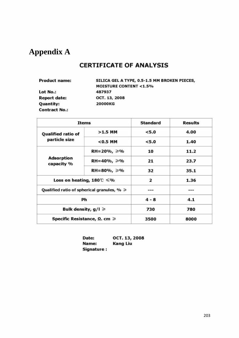
203
Appendix A
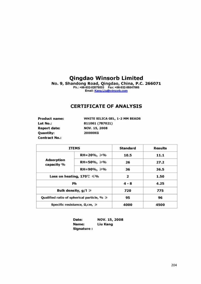
204
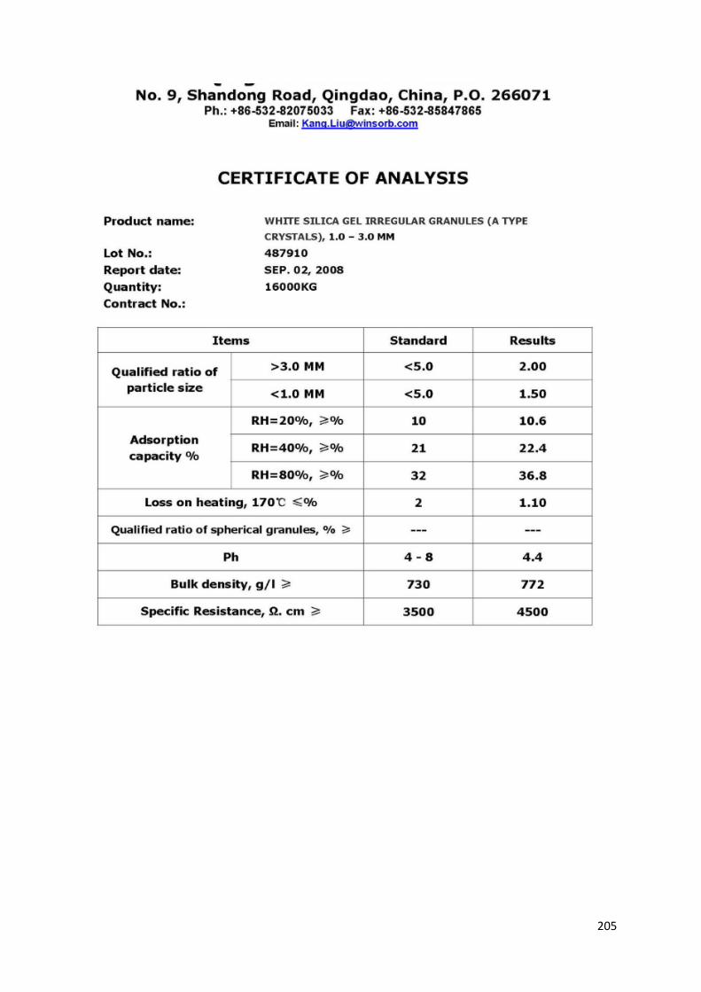
205
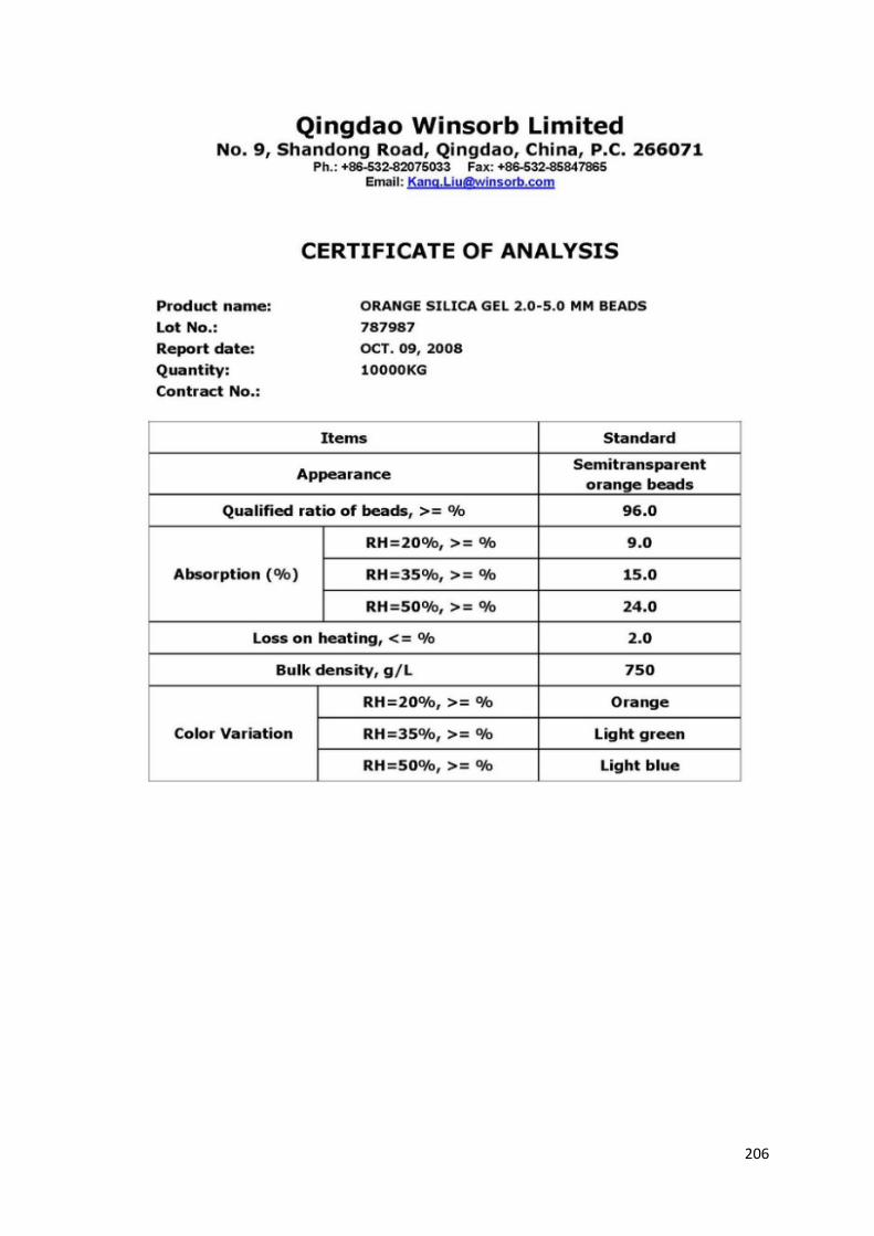
206
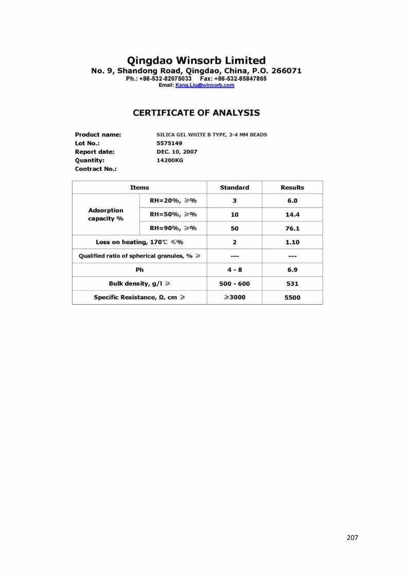
207
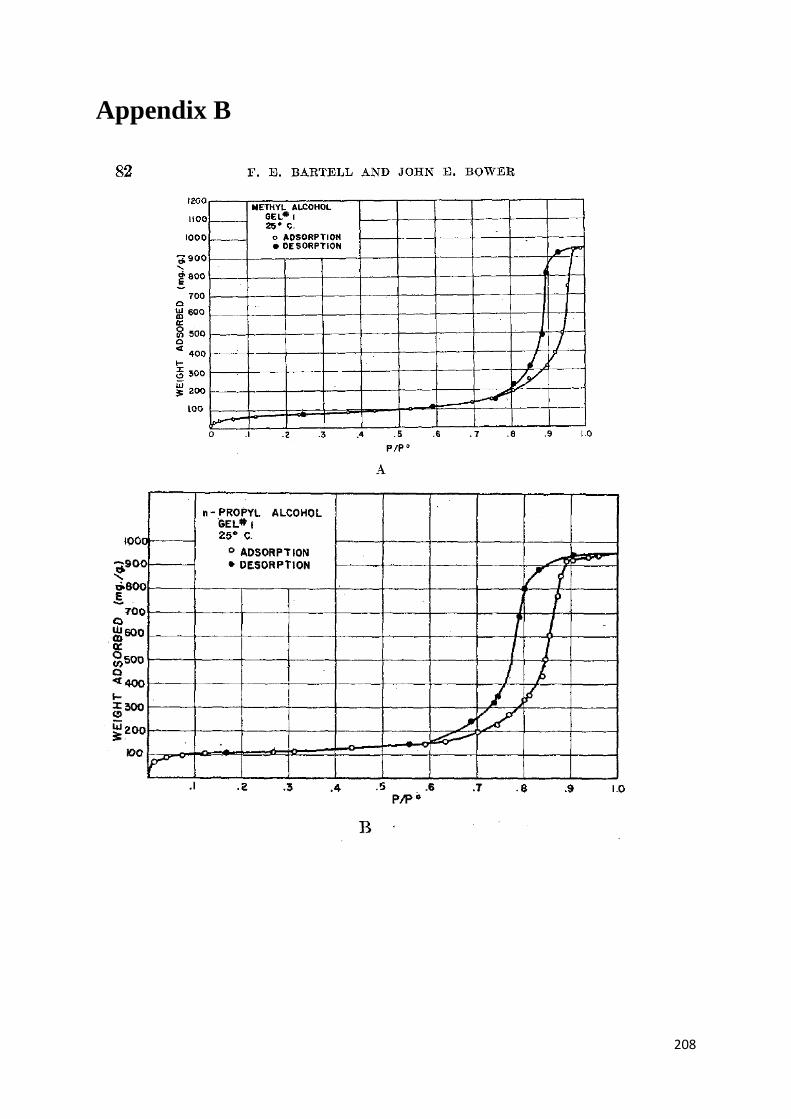
208
Appendix B
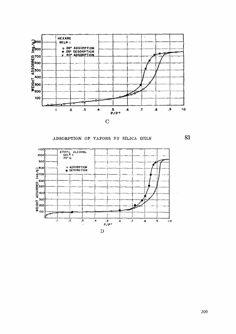
209
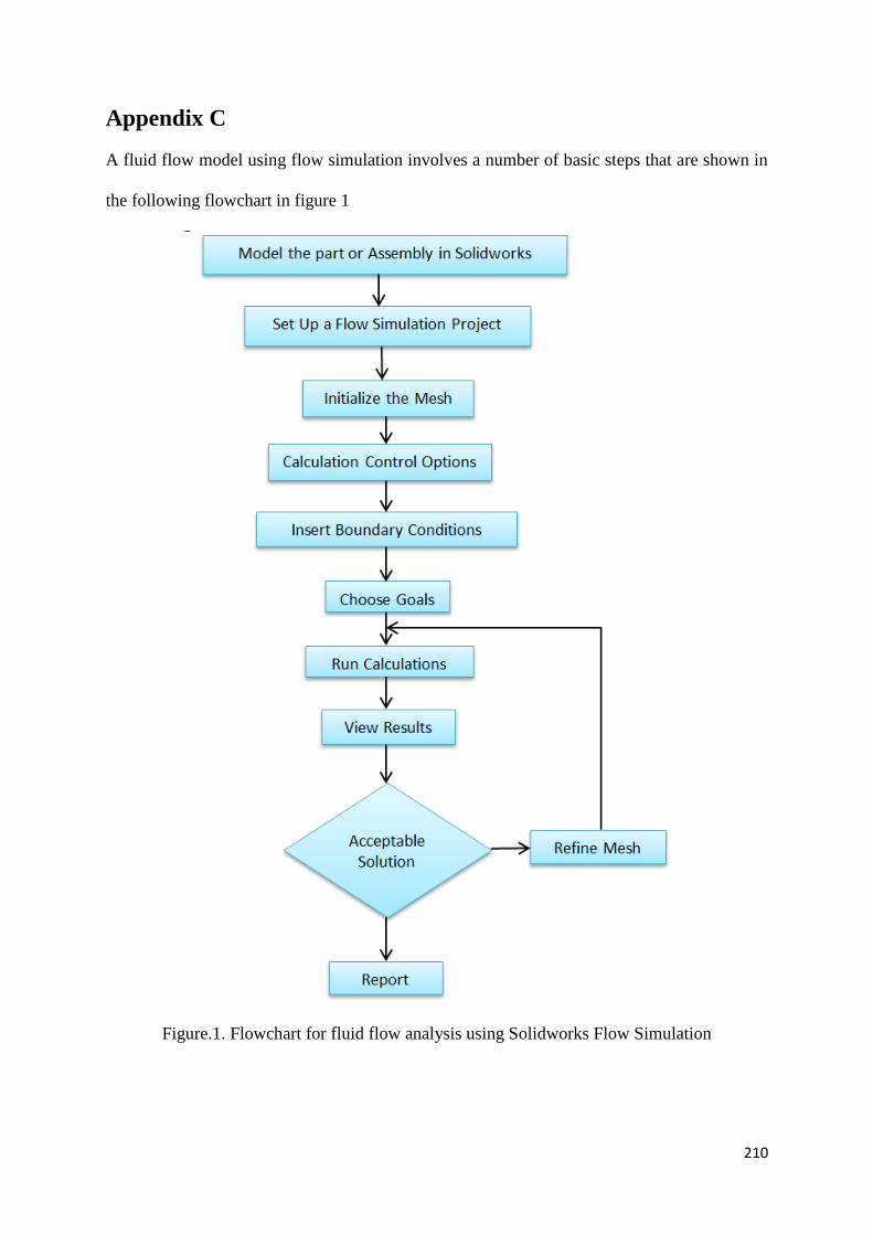
210
Appendix C
A fluid flow model using flow simulation involves a number of basic steps that are shown in
the following flowchart in figure 1
Figure.1. Flowchart for fluid flow analysis using Solidworks Flow Simulation