CFD SIMULATION OF CRUDE OIL HOMOGENIZATION IN PILOT … · CFD SIMULATION OF CRUDE OIL HOMOGENIZATION IN PILOT PLANT SCALE CT&F - Ciencia, Tecnología y Futuro - Vol. 5 Num. 2 Jun

CFD SIMULATION OF CRUDE OIL HOMOGENIZATION IN PILOT PLANT SCALE

CT&F - Ciencia, Tecnología y Futuro - Vol. 5 Num. 2 Jun. 2013 19

CFD SIMULATION OF CRUDE OIL HOMOGENIZATION IN PILOT

PLANT SCALE

Jesús-Alberto Castro-Gualdrón1*, Leonel-Andrés Abreu-Mora1 and Fabián-Andrey Díaz-Mateus2*

1Ecopetrol S.A. - Instituto Colombiano del Petróleo (ICP), A.A. 4185 Bucaramanga, Santander, Colombia2Ambiocoop Ltda. Bucaramanga, Santander, Colombia

e-mail: [email protected] [email protected]

(Received: Sep. 24, 2012; Accepted: May 17, 2013)

Keywords: Hydrocarbons, Blending, Tank, Agitation, Impeller.

*To whom correspondence should be addressed

CT&F - Ciencia, Tecnología y Futuro - Vol. 5 Num. 2 Jun. 2013 Pag. 19 - 30

The homogenization of different crude oils in a pilot plant tank is simulated using Computational Fluid Dynamics (CFD) commercial code. The models are inherently transient since all simulations start from a time zero where the crudes are completely separated to a final time of full homogenization. The tank

is agitated with a small impeller and a two-phase model is used in the simulations in order to see the mixing process and calculate the properties of the blend based on the volume fractions. The effect of the mesh size and time step size are studied since in this type of simulations the computational effort becomes a major pa-rameter and has to be reduced to a minimum. Experimental data taken from two different points in the tank at regular time intervals are available to compare the results of the simulations, concluding in good agreement.

ABSTRACT

How to cite: Castro-Gualdrón, J. A., Díaz-Mateus, F. A. & Abreu-Mora, L. A. (2013). CFD simulation of crude oil homogenization in pilot plant scale. CT&F - Ciencia, Tecnología y Futuro, 5(2), 19-30.

SIMULACIÓN MEDIANTE CFD DE LA HOMOGENIZACIÓN DE CRUDOS A ESCALA PILOTO

ISSN 0122-5383Latinoamerican journal of oil & gas and alternative energy

CT&F - Ciencia, Tecnología y Futuro - Vol. 5 Num. 2 Jun. 2013

JESÚS-ALBERTO CASTRO-GUALDRÓN et al.

20

A homogeneização de diferentes crus em tanque a escala piloto é simulada usando código comer-cial para Dinâmica Computacional de Fluidos - por sua sigla em inglês (CFD). Os modelos são inerentemente dinâmicos já que todas as simulações partem de um tempo zero onde os crus estão

completamente separados até um tempo final de completa homogeneização. O tanque é agitado com uma pequena hélice e um modelo de duas fases é usado na simulação com o propósito de observar o processo de mistura e calcular as propriedades da mistura em função das frações volumétricas. O efeito do tamanho de malha e a passagem do tempo são estudados, pois neste tipo de simulações o esforço computacional se converte em um parâmetro muito importante e deve ser reduzido ao mínimo. Dados experimentais tomados em dois pontos diferentes dentro do tanque em intervalos regulares de tempo estão disponíveis e observa-se boa concordância quando comparados com os resultados das simulações.

L a homogenización de diferentes crudos en tanque a escala piloto es simulada usando código co-mercial para Dinámica Computacional de Fluidos - de sus siglas en inglés (CFD). Los modelos son inherentemente dinámicos ya que todas las simulaciones parten de un tiempo cero donde los crudos

se encuentran completamente separados hasta un tiempo final de completa homogenización. El tanque es agitado con una pequeña propela y un modelo de dos fases es usado en la simulación con el propósito de observar el proceso de mezclado y calcular las propiedades de la mezcla en función de las fracciones volumétricas. El efecto del tamaño de malla y el paso en el tiempo son estudiados pues en este tipo de simulaciones el esfuerzo computacional se convierte en un parámetro muy importante y debe ser reducido al mínimo. Datos experimentales tomados en dos puntos diferentes dentro del tanque a intervalos regulares de tiempo están disponibles y se observa buena concordancia cuando se comparan con los resultados de las simulaciones.

Palabras clave: Hidrocarburos, Mezcla, Tanque, Agitación, Propela.

Palavras-chave: Hidrocarbonetos, Mistura, Tanque, Agitação, Hélice.

RESUMEN

RESUMO



1. INTRODUCTION

The homogenization time in crude oil storage tanks is a very important parameter in refineries where different crudes are charged continuously and the homogeneity of the crude stocks is necessary to assure a good perfor-mance of the refinery processes. In production locations heavy oils are usually mixed with lighter ones to achieve a proper viscosity for transportation in pipelines. In re-fineries such as Barrancabermeja Refinery (Barrancaber-meja, Colombia), several crudes that come from many places are pumped into the storage tanks and mixed in order to achieve a blend with suitable properties to be fed into the distillation units.

The mixing process inside storage tanks is usually unknown and the crude has different properties de-pending on the place where is pumped out. With CFD simulations, all the properties of the blend can be con-tinuously observed throughout the entire tank. Different geometries can be simulated, different impellers, jets or layouts can be analyzed and the consumption of energy for mixing can be optimized.

A CFD simulation must follow the next main steps: Construction of the Computer Aided Design (CAD) geo-metry and meshing, definition of mathematical models, resolution of equations and post-processing of results. Due to the complex shapes that mixers in agitated tanks have, the meshing usually results in a combination of tetrahedral, wedge and hexahedral forms. Thus, the flow is never aligned with the mesh and second order dis-cretization or higher must be used to solve the equations. In the post-processing is usual to refine the mesh in the proximities of the mixer where the gradients are several times higher to the rest of the tank. Refining the mesh reduces the false numerical diffusion and interpolation errors as its seen elsewhere in this publication.

CFD has been widely used to simulate mixing pro-cesses due to its capability to predict the transient varia-tion of different parameters and the capacity to analyze every type of vessel and mixers. Several researchers such as Marshall and Bakker (2003) and Fernandes, Cekinski, Nunhez and Urenha (2007) have simulated different configurations of mixers in tanks for industrial applications.

Few publications in the literature are found when it comes to mixing of crude oils using CFD. Dakhel and Rahimi (2004), Rahimi (2005) and Rahimi and Parvareh (2005) simulated the mixing process of light crude oils in storage tanks by impellers or jets. However, a two phase model is not presented and is not clear in these publications how the properties of the blend are calculated.

In this work the term blend refers to the mixture of hydrocarbons with different properties. The accu-rate calculation of blend properties is very important in industrial hydrocarbon applications where certain parameter must be assured such as a specific value of viscosity or density. It is well known that the calcula-tion of blend properties is not straightforward and different methods are available in the literature to calculate densities or viscosities of mixtures. In this work, different methods will be analyzed and a mul-tiphase model for miscible fluids is used in the CFD code where each hydrocarbon corresponds to a liquid phase in the multiphase model.

2. EXPERIMENTAL DEVELOPMENT

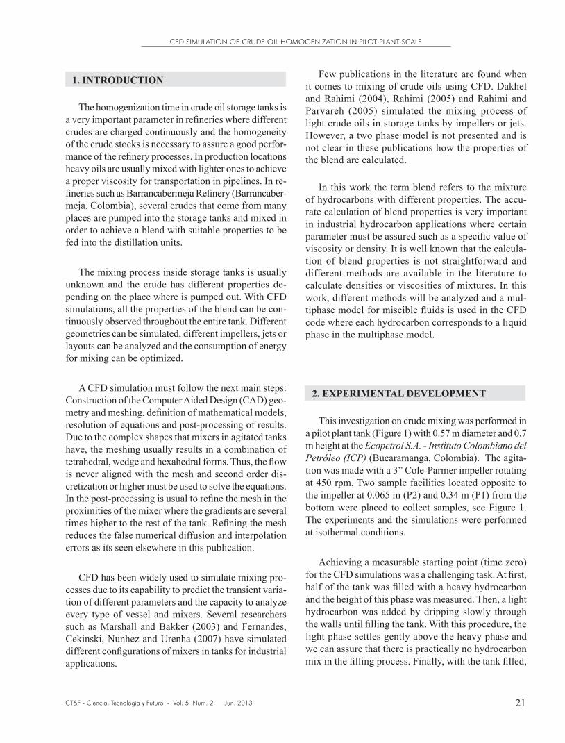
This investigation on crude mixing was performed in a pilot plant tank (Figure 1) with 0.57 m diameter and 0.7 m height at the Ecopetrol S.A. - Instituto Colombiano del Petróleo (ICP) (Bucaramanga, Colombia). The agita-tion was made with a 3” Cole-Parmer impeller rotating at 450 rpm. Two sample facilities located opposite to the impeller at 0.065 m (P2) and 0.34 m (P1) from the bottom were placed to collect samples, see Figure 1. The experiments and the simulations were performed at isothermal conditions.

Achieving a measurable starting point (time zero) for the CFD simulations was a challenging task. At first, half of the tank was filled with a heavy hydrocarbon and the height of this phase was measured. Then, a light hydrocarbon was added by dripping slowly through the walls until filling the tank. With this procedure, the light phase settles gently above the heavy phase and we can assure that there is practically no hydrocarbon mix in the filling process. Finally, with the tank filled,



22

Figure 1. Geometry of the pilot tank where the experiments were performed.

3. GEOMETRY AND MESHING

Two different and independent volumes were cons-tructed: one for the cylinder that contains the impeller and another one for the rest of the tank; both volumes are connected by a grid interface. The cylinder was made surrounding the impeller in the smallest po-ssible size that permitted a tetrahedral mesh with all elements having an equisize skew below 0.8. The rest of the domain was meshed with hexahedral elements. The k-ε turbulence models require maintaining the y+ coefficient between 30 - 300 in order to use the standard wall functions as proposed by Launder and Spalding (1974). Thus, the boundary layer cells in the proximities of the walls were rigorously sized to fulfill this constraint, see Figure 2. The k-ε turbulence model used in this work will be discussed in the next chapter. Nunhez (1994) and Fernandes et al. (2007) found that

tetrahedral meshes without proper boundary layers at the walls led to numerical errors as seen on Figure 3 where the contours of velocity present an oscillation bordering the walls of the tank.

Figure 2. Meshing for the impeller and the tank.

Figure 3. Errors in the contours of velocity found in tetrahedral meshes (Fernandes et al., 2007).

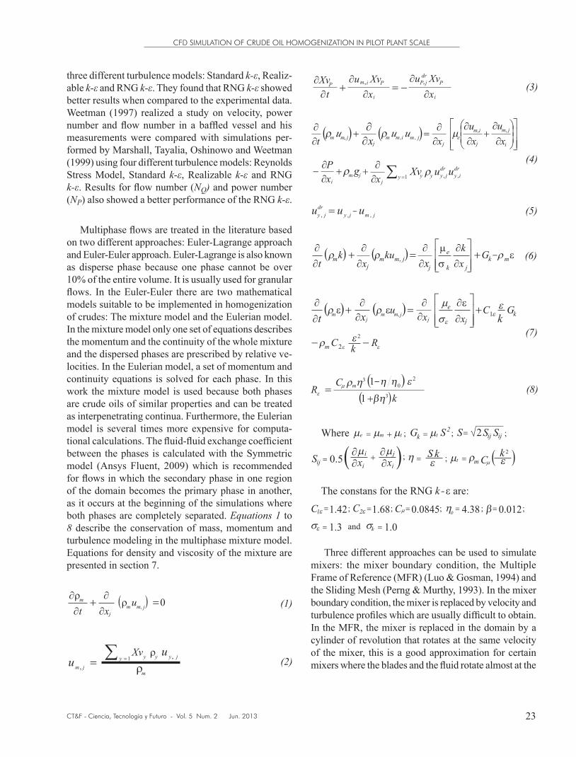
4. MATHEMATICAL MODELS

The equations that describe the three dimensional transient fluid flow in an agitated tank is Reynolds Average Navier Stokes (RANS) based, the flow can be considered incompressible since high Mach numbers are not presented. For turbulence modeling, the Re-normalization Group (RNG) k-ε was selected with the cons-tants and equations as presented by Yakhot and Orszag (1986). Rahimi and Parvareh (2005) presented a study in a semi-industrial tank on mixing by jets using

Sample facility P1

Propeller

Sample facility P2

0.57 m0.36 m

0.275 m

0.065 m

the experiment may start from a time zero where both hydrocarbons are completely separated. Once the im-peller is turned on, the mixing process starts and samples were taken at regular time intervals. The experimental procedures were simulated using CFD through the software Ansys FluentTM 12.0.



three different turbulence models: Standard k-ε, Realiz-able k-ε and RNG k-ε. They found that RNG k-ε showed better results when compared to the experimental data. Weetman (1997) realized a study on velocity, power number and flow number in a baffled vessel and his measurements were compared with simulations per-formed by Marshall, Tayalia, Oshinowo and Weetman (1999) using four different turbulence models: Reynolds Stress Model, Standard k-ε, Realizable k-ε and RNG k-ε. Results for flow number (NQ) and power number (NP) also showed a better performance of the RNG k-ε.

Multiphase flows are treated in the literature based on two different approaches: Euler-Lagrange approach and Euler-Euler approach. Euler-Lagrange is also known as disperse phase because one phase cannot be over 10% of the entire volume. It is usually used for granular flows. In the Euler-Euler there are two mathematical models suitable to be implemented in homogenization of crudes: The mixture model and the Eulerian model. In the mixture model only one set of equations describes the momentum and the continuity of the whole mixture and the dispersed phases are prescribed by relative ve-locities. In the Eulerian model, a set of momentum and continuity equations is solved for each phase. In this work the mixture model is used because both phases are crude oils of similar properties and can be treated as interpenetrating continua. Furthermore, the Eulerian model is several times more expensive for computa-tional calculations. The fluid-fluid exchange coefficient between the phases is calculated with the Symmetric model (Ansys Fluent, 2009) which is recommended for flows in which the secondary phase in one region of the domain becomes the primary phase in another, as it occurs at the beginning of the simulations where both phases are completely separated. Equations 1 to 8 describe the conservation of mass, momentum and turbulence modeling in the multiphase mixture model. Equations for density and viscosity of the mixture are presented in section 7.

0,�

�

��

�

�jmm

j

m uxt

�� (1)

y jyyy

jm

uXvu

m�

��1 ,

,(2)

P

dr

jPPimPXvuXvu

t

Xv ��

ix�

��

�

� ,,

ix�(3)

j

im

ej

jmimj

jmmx

u

xuu

xu

t,

,,,

��

�

��

�

��

�

�

��

�

�

ix�jmu ,�

��

�

�

��

�

��

�

�

dr

iy

dr

jyy yyj

uuXvx ,,1��

�� jm

i

gx

P�

�

��

�� m �

(4)

jmjy

dr

jy uuu ,,, �� (5)

� ��

�� mk

jk

e

j

jmmm Gx

k

xkuk

t��

��

�

��

�

�

�

�

��

jx�

��

�

�, �� (6)

� ��

��

�

�� G

kC

xxu

xtk

j

e

jjmm

jm

��

�

��

�

�

�

�

��

�

��

�

�

��

�� Rk

Cm ��2

2

1,� � �

(7)

CR

m 1 20

3 �� k1 3��

�� (8)

me ��t��kG S�t�2�S�2Sij SijWhere �

Sij �0.5 ��i

��j

�xi

��S k��t��m C��k 2

��

The constans for the RNG k are:�

C��1.42�C��1.68�C��0.0845��4.38��0.012�

��1.3 ��1.0kand

xi

Three different approaches can be used to simulate mixers: the mixer boundary condition, the Multiple Frame of Reference (MFR) (Luo & Gosman, 1994) and the Sliding Mesh (Perng & Murthy, 1993). In the mixer boundary condition, the mixer is replaced by velocity and turbulence profiles which are usually difficult to obtain. In the MFR, the mixer is replaced in the domain by a cylinder of revolution that rotates at the same velocity of the mixer, this is a good approximation for certain mixers where the blades and the fluid rotate almost at the



24

same velocity and there is a weak interaction between the blades and the rest of the tank. A simulation with MFR is more appropriate for steady solutions, since the mixer is static in the simulation. In the sliding mesh, a cylinder of revolution must be also built, but the mixer inside does rotate and interact with the fluid and the rest of the tank. The information from inside the cylinder is exchanged to rest of the domain by a grid interface between both. The sliding mesh method is more appropriate for transient solutions and is used in this work.

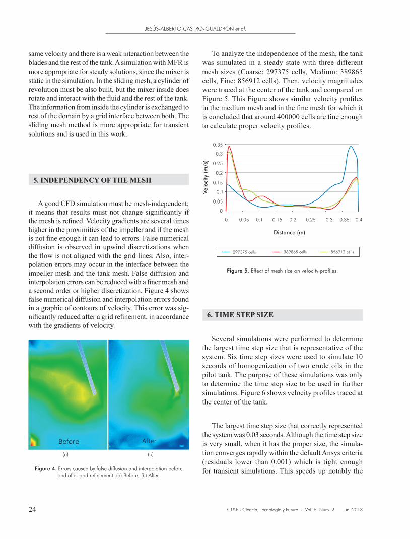
5. INDEPENDENCY OF THE MESH

A good CFD simulation must be mesh-independent; it means that results must not change significantly if the mesh is refined. Velocity gradients are several times higher in the proximities of the impeller and if the mesh is not fine enough it can lead to errors. False numerical diffusion is observed in upwind discretizations when the flow is not aligned with the grid lines. Also, inter-polation errors may occur in the interface between the impeller mesh and the tank mesh. False diffusion and interpolation errors can be reduced with a finer mesh and a second order or higher discretization. Figure 4 shows false numerical diffusion and interpolation errors found in a graphic of contours of velocity. This error was sig-nificantly reduced after a grid refinement, in accordance with the gradients of velocity.

Figure 4. Errors caused by false diffusion and interpolation before and after grid refinement. (a) Before, (b) After.

To analyze the independence of the mesh, the tank was simulated in a steady state with three different mesh sizes (Coarse: 297375 cells, Medium: 389865 cells, Fine: 856912 cells). Then, velocity magnitudes were traced at the center of the tank and compared on Figure 5. This Figure shows similar velocity profiles in the medium mesh and in the fine mesh for which it is concluded that around 400000 cells are fine enough to calculate proper velocity profiles.

0.05 0.1 0.15 0.2 0.25 0.3 0.35 0.4

Distance (m)

0

297375 cells 389865 cells 856912 cells

0.35

0.3

0.25

0.2

0.15

0.1

0.05

0Velo

city

(m

/s)

Figure 5. Effect of mesh size on velocity profiles.

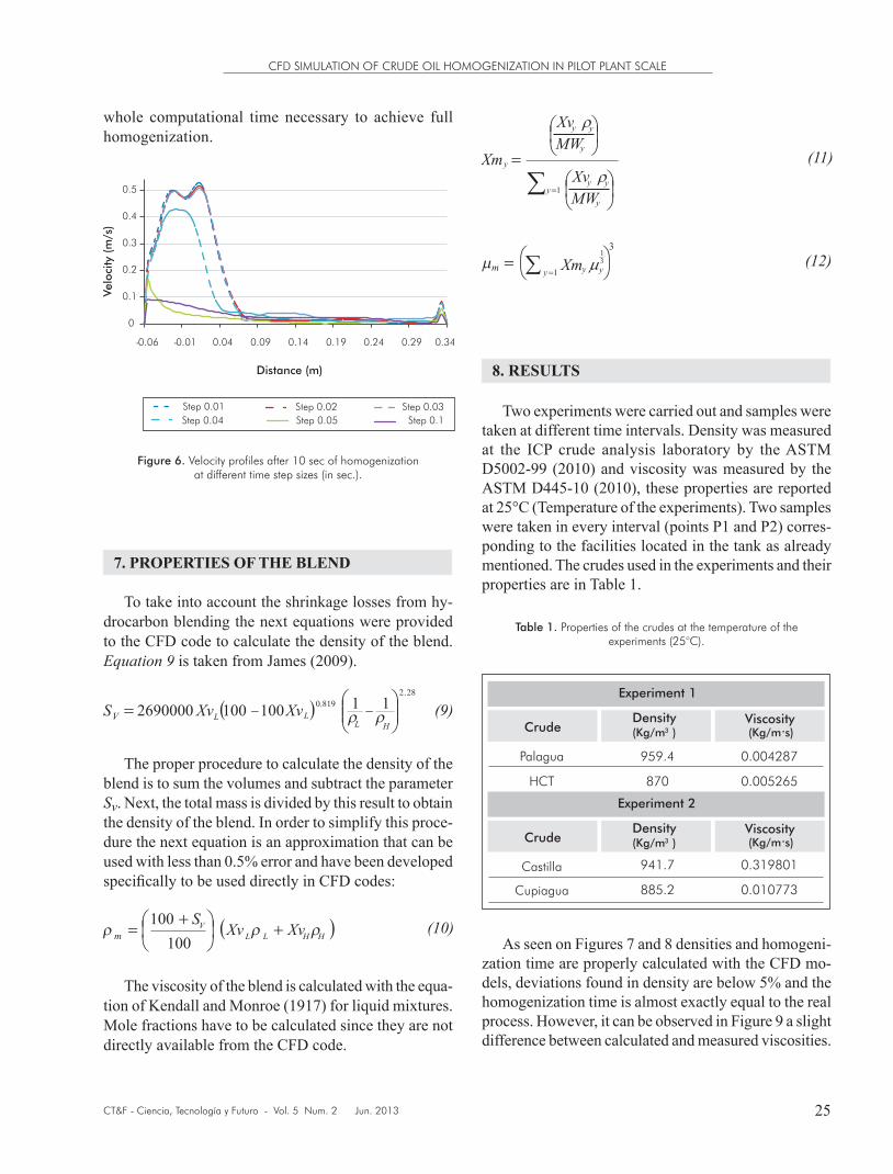
6. TIME STEP SIZE

Several simulations were performed to determine the largest time step size that is representative of the system. Six time step sizes were used to simulate 10 seconds of homogenization of two crude oils in the pilot tank. The purpose of these simulations was only to determine the time step size to be used in further simulations. Figure 6 shows velocity profiles traced at the center of the tank.

The largest time step size that correctly represented the system was 0.03 seconds. Although the time step size is very small, when it has the proper size, the simula-tion converges rapidly within the default Ansys criteria (residuals lower than 0.001) which is tight enough for transient simulations. This speeds up notably the

(a) (b)



whole computational time necessary to achieve full homogenization.

0

0.1

0.2

0.3

0.4

0.5

-0.06 -0.01 0.04 0.09 0.14 0.19 0.24 0.29 0.34

Velo

city

(m

/s)

Distance (m)

Step 0.01

Step 0.1Step 0.04

Step 0.02 Step 0.03

Step 0.05

Figure 6. Velocity profiles after 10 sec of homogenization at different time step sizes (in sec.).

7. PROPERTIES OF THE BLEND

To take into account the shrinkage losses from hy-drocarbon blending the next equations were provided to the CFD code to calculate the density of the blend. Equation 9 is taken from James (2009).

� 0.819 1001002690000 �� LLV XvXvS �

28.2

11��

��

L��

�

�

H� (9)

The proper procedure to calculate the density of the blend is to sum the volumes and subtract the parameter Sv. Next, the total mass is divided by this result to obtain the density of the blend. In order to simplify this proce-dure the next equation is an approximation that can be used with less than 0.5% error and have been developed specifically to be used directly in CFD codes:

�HHLL

Vm XvXv

S��

�

��

��

100

100 � (10)

The viscosity of the blend is calculated with the equa-tion of Kendall and Monroe (1917) for liquid mixtures. Mole fractions have to be calculated since they are not directly available from the CFD code.

��

�

1y

yXm (11)

��

�yMW

yyXv ��

�

��

�yMW

yyXv ��

�

3

1��y yym Xm �� 3

1�

�� (12)

8. RESULTS

Two experiments were carried out and samples were taken at different time intervals. Density was measured at the ICP crude analysis laboratory by the ASTM D5002-99 (2010) and viscosity was measured by the ASTM D445-10 (2010), these properties are reported at 25°C (Temperature of the experiments). Two samples were taken in every interval (points P1 and P2) corres-ponding to the facilities located in the tank as already mentioned. The crudes used in the experiments and their properties are in Table 1.

Table 1. Properties of the crudes at the temperature of the experiments (25°C).

Experiment 1

Palagua

HCT

CrudeDensity

3(Kg/m )Viscosity

Experiment 2

Castilla

Cupiagua

CrudeDensity

3(Kg/m )

.(Kg/m s)

Viscosity.(Kg/m s)

959.4

870

0.004287

0.005265

941.7

885.2

0.319801

0.010773

As seen on Figures 7 and 8 densities and homogeni-zation time are properly calculated with the CFD mo-dels, deviations found in density are below 5% and the homogenization time is almost exactly equal to the real process. However, it can be observed in Figure 9 a slight difference between calculated and measured viscosities.



26

960

950

940

930

920

910

900

880

870

0 2 4 6 8 10

Time (min)

3D

ensi

ty (

Kg/m

)

Measured P1 Measured P2

Calculated P1 Calculated P2

Figure 7. Variation in time of the crude blend density for experiment 1.

Figure 8. Variation in time of the crude blend density for experiment 2.

0

0.05

0.1

0.15

0.2

0.25

0.3

0.35

0 5 10 15 20

Vis

cosi

ty (

kg/m

s)

Time (min)

Measured P2 Measured P2

Calculated P1 Calculated P2

Figure 9. Variation in time of the crude blend viscosity for experiment 2.

It is known that calculating accurate viscosities of hydrocarbon blends is a difficult task; nevertheless, de-viations are maximum at 22%, which is very different to the 400% calculated with Equation 13, a method used by CFD commercial codes to calculate viscosity of mixtures.

�m1��y yyXv �� (13)

Table 2. Deviations found in viscosity (kg/m•s) of the full blend of crudes in experiment 2.

MeasuredCalculated Equations

11, 12

Deviation

%

Calculated Equation

13

Deviation

%

912.4 912.29912.38 0.02 0.1

Table 2 shows the difference between the method

used by commercial CFD codes and the method used in this work to calculate viscosity of mixtures. Viscosi-ties found with Equation 13 are exceedingly different to measured values, while Equations 11 and 12 show an excellent approximation to the real value.

The method used by CFD commercial codes to cal-culate density of mixtures is the same used to calculate viscosity, as seen on Equation 14.

(14)�m1��y yyXv� �

Table 3. Deviations found in density (kg/m3) of the full blend of crudes in experiment 2.

MeasuredCalculated Equations

9, 10

Deviation

%

Calculated Equation

14

Deviation

%

912.4 912.29912.38 0.02 0.1

Table 3 shows that differences between the method used by commercial CFD codes and the method used in this work to calculate density of mixtures seem in-significant due to the small size of the pilot tank used to perform the experiments. However, when it comes to blending of crudes in industrial refinery tanks, these differences become very significant due to the important shrinkage in the volume of the blend, see James (2009).



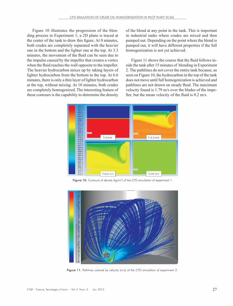
Figure 10 illustrates the progression of the blen-ding process in Experiment 1; a 2D plane is traced at the center of the tank to draw this figure. At 0 minutes, both crudes are completely separated with the heavier one in the bottom and the lighter one at the top. At 3.3 minutes, the movement of the fluid can be seen due to the impulse caused by the impeller that creates a vortex when the fluid reaches the wall opposite to the impeller. The heavier hydrocarbon mixes up by taking layers of lighter hydrocarbon from the bottom to the top. At 6.6 minutes, there is only a thin layer of lighter hydrocarbon at the top, without mixing. At 10 minutes, both crudes are completely homogenized. The interesting feature of these contours is the capability to determine the density

of the blend at any point in the tank. This is important in industrial tanks where crudes are mixed and then pumped out. Depending on the point where the blend is pumped out, it will have different properties if the full homogenization is not yet achieved.

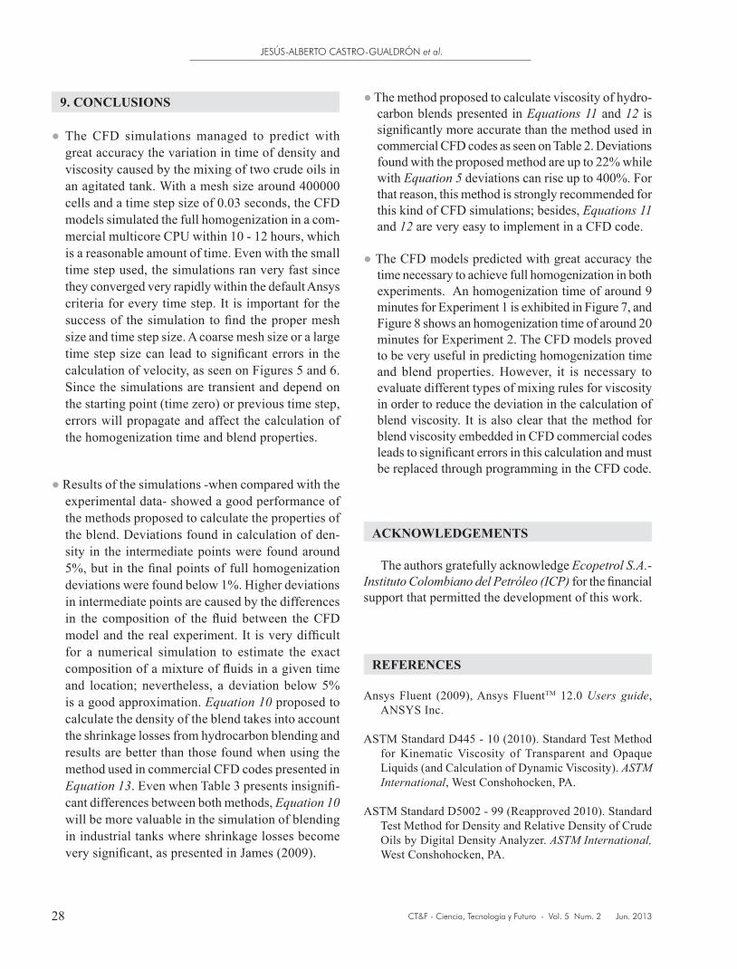
Figure 11 shows the course that the fluid follows in-side the tank after 15 minutes of blending in Experiment 2. The pathlines do not cover the entire tank because, as seen on Figure 10, the hydrocarbon in the top of the tank does not move until full homogenization is achieved and pathlines are not drawn on steady fluid. The maximum velocity found is 1.79 m/s over the blades of the impe-ller, but the mean velocity of the fluid is 0.2 m/s.

Figure 10. Contours of density (kg/m3) of the CFD simulation of experiment 1.

Figure 11. Pathlines colored by velocity (m/s) of the CFD simulation of experiment 2.



28

9. CONCLUSIONS

● The CFD simulations managed to predict with great accuracy the variation in time of density and viscosity caused by the mixing of two crude oils in an agitated tank. With a mesh size around 400000 cells and a time step size of 0.03 seconds, the CFD models simulated the full homogenization in a com-mercial multicore CPU within 10 - 12 hours, which is a reasonable amount of time. Even with the small time step used, the simulations ran very fast since they converged very rapidly within the default Ansys criteria for every time step. It is important for the success of the simulation to find the proper mesh size and time step size. A coarse mesh size or a large time step size can lead to significant errors in the calculation of velocity, as seen on Figures 5 and 6. Since the simulations are transient and depend on the starting point (time zero) or previous time step, errors will propagate and affect the calculation of the homogenization time and blend properties.

● Results of the simulations -when compared with the experimental data- showed a good performance of the methods proposed to calculate the properties of the blend. Deviations found in calculation of den-sity in the intermediate points were found around 5%, but in the final points of full homogenization deviations were found below 1%. Higher deviations in intermediate points are caused by the differences in the composition of the fluid between the CFD model and the real experiment. It is very difficult for a numerical simulation to estimate the exact composition of a mixture of fluids in a given time and location; nevertheless, a deviation below 5% is a good approximation. Equation 10 proposed to calculate the density of the blend takes into account the shrinkage losses from hydrocarbon blending and results are better than those found when using the method used in commercial CFD codes presented in Equation 13. Even when Table 3 presents insignifi-cant differences between both methods, Equation 10 will be more valuable in the simulation of blending in industrial tanks where shrinkage losses become very significant, as presented in James (2009).

● The method proposed to calculate viscosity of hydro-carbon blends presented in Equations 11 and 12 is significantly more accurate than the method used in commercial CFD codes as seen on Table 2. Deviations found with the proposed method are up to 22% while with Equation 5 deviations can rise up to 400%. For that reason, this method is strongly recommended for this kind of CFD simulations; besides, Equations 11 and 12 are very easy to implement in a CFD code.

● The CFD models predicted with great accuracy the time necessary to achieve full homogenization in both experiments. An homogenization time of around 9 minutes for Experiment 1 is exhibited in Figure 7, and Figure 8 shows an homogenization time of around 20 minutes for Experiment 2. The CFD models proved to be very useful in predicting homogenization time and blend properties. However, it is necessary to evaluate different types of mixing rules for viscosity in order to reduce the deviation in the calculation of blend viscosity. It is also clear that the method for blend viscosity embedded in CFD commercial codes leads to significant errors in this calculation and must be replaced through programming in the CFD code.

ACKNOWLEDGEMENTS

The authors gratefully acknowledge Ecopetrol S.A.-Instituto Colombiano del Petróleo (ICP) for the financial support that permitted the development of this work.

REFERENCES

Ansys Fluent (2009), Ansys FluentTM 12.0 Users guide, ANSYS Inc.

ASTM Standard D445 - 10 (2010). Standard Test Method for Kinematic Viscosity of Transparent and Opaque Liquids (and Calculation of Dynamic Viscosity). ASTM International, West Conshohocken, PA.

ASTM Standard D5002 - 99 (Reapproved 2010). Standard Test Method for Density and Relative Density of Crude Oils by Digital Density Analyzer. ASTM International, West Conshohocken, PA.



Dakhel, A. A. & Rahimi, M. (2004). CFD simulation of homogenization in large-scale crude oil storage tanks. J. Pet. Sci. Eng., 43(3-4), 151 - 161.

Fernandes, C., Cekinski, E., Nunhez, J. R. & Urenha, L. C. (2007). Agitação e Mistura na Industria. Brazil: LTC Ed

James, H. (2009). Shrinkage losses resulting from liquid hydrocarbon blending. Alberta: J2 Measurement Solu-tions Inc. Clearwater B.C.

Kendall, J. & Monroe, K. P. (1917). The viscosity of liquids II. The viscosity composition curve for ideal liquid mix-tures. J. Am. Chem. Soc., 39(9), 1787-1802.

Launder, B. E. & Spalding, D. B. (1974). The numerical computation of turbulent flows. Comput. Methods Appl. Mech. Eng., 3(2), 269-289.

Luo, J. Y., Issa, R. I. & Gosman, A. D. (1994). Prediction of impeller induced flows in mixing vessels using multiple frames of reference. 8th Europe Conference on Mixing, Inst. Chem. Eng. Symp. Ser., Cambridge, UK. No. 136.

Marshall, E. M. & Bakker, A. (2003). Computational fluid mixing. Lebanon: Fluent Inc.

Marshall, E. M., Tayalia, Y., Oshinowo, L. & Weetman, R. (1999). Comparison of turbulence models in CFD predictions of flow number and power draw in stirred tanks, Mixing XVII, Banff, Alberta, Canadá.

Nunhez, J. R. (1994). The influence of geometric factors on the optimum design of stirred tank reactors. Ph. D. Thesis, University of Leeds, Leeds , UK.

Perng, C. Y. & Murthy J. Y. (1993). A moving - deforming-mesh technique for simulation of flow in mixing tanks. Process Mixing - Chemical and biochemical applica-tions: Part II. AICHE Symp. Ser. 211(293), 37-41.

Rahimi, M. (2005). The effect of impellers layout on mixing time in a large-scale crude oil storage tank. J. Pet. Sci. Eng., 46(3), 161-170.

Rahimi, M. & Parvareh, A. (2005). Experimental and CFD investigation on mixing by a jet in a semi-industrial stirred tank. Chem. Eng. J., 115(1-2), 85-92.

Weetman, R. J. (1997). Automated sliding mesh CFD compu-tations for fluid foil impellers, 9th European Conference on Mixing, Paris, France.

Yakhot, V. & Orszag, S. A. (1986). Renormalization group analysis of turbulence. I. Basic theory. J. Sci. Comput., 1(1), 3-51.

AUTHORS

Jesús-Alberto Castro-Gualdrón.

Affiliation: Ecopetrol S.A. - Instituto Colombiano del Petróleo (ICP).Ing. Química, M.Sc. Ing. Química, Universidad Industrial de Santander; Esp. Gerencia de Recursos Energéticos, Universidad Autónoma de Bucaramanga.e-mail: [email protected]

Fabián-Andrey Díaz-Mateus.Affiliation: Ambiocoop Ltda.

Ing. Química, Universidad Industrial de Santander; M.Sc, Univer-sidad de Campinas.e-mail: [email protected]

Leonel-Andres Abreu-Mora.

Affiliation: Ecopetrol S.A. - Instituto Colombiano del Petróleo (ICP).Ing. Química, Esp. Auditorias de Seguridad de Procesos.e-mail: [email protected]



30

C , C , C , ç ,â2å ì 1å 0

gj

Gk

k

MWy

P

Rå

S Sij

SV

udr

P,i,j

udry,i,j

ui,j

um,i,j

xi,j

Xmy

Xvy, P, L, H

Constants for the RNG k - å model

2Gravity in the j direction (m/s )

3Production of turbulent kinetic energy term (J/m /s)2 2Turbulent kinetic energy per unit mass (m /s )

Molecular Weight of phase y

Absolute pressure (Pa)

RNG term in the RNG k - å model- 1

Inverse of the mean shear time scale (s )

Mean strain rate tensor

Volumetric shrinkage, as a % of the total mixture

ideal volume

Drift velocity of the secondary phase in the i, j

direction (m/s)

Drift velocity of phase y in the i, j direction (m/s)

Velocity component in the i, j direction (m/s)

Velocity component of the mixture in the i, j

direction (m/s)

Coordinate in the i, j direction

Molar fraction of phase y

Volume fraction of phase y, secondary phase, lighter

component, heavier component

å

ç�,e ��,t ��m

�,�m ,�L, Hy

��

GREEK LETTERS

NOTATION

Dissipation rate of turbulent kinetic energy per unit 2 3mass (m /s )

Turbulence to mean shear time scale ratio

Effective, Turbulent and Molecular viscosity of .the mixture (Pa s)

Density of the mixture, phase y, lighter component, 3heavier component (kg/m )

Turbulent Prandtl number for k and å

Documents

CFD SIMULATION OF CRUDE OIL HOMOGENIZATION IN PILOT … · CFD SIMULATION OF CRUDE OIL HOMOGENIZATION IN PILOT PLANT SCALE CT&F - Ciencia, Tecnología y Futuro - Vol. 5 Num. 2 Jun