CFD SIMULATION OF A SOLID BOWL CENTRIFUGE

USED FOR WASTE MANAGEMENT

Dipl.-Ing. X. Romaní Fernández; Prof. Dr.-Ing. H. Nirschl

Universität Karlsruhe (TH), Institut für MVM

E-mail: xiana.romani@mvm.uni-karlsruhe.de

ABSTRACT

This study presents some initial results from the numerical simulation of the flow in a solid

bowl centrifuge used for the particle separation in the industrial fluid processing. Fluent,

Computational Fluid Dynamics (CFD) software was used to simulate this multiphase flow.

Simplified two dimensional and three dimensional geometries were built and meshed from the

real centrifuge geometry. The CFD results showed a boundary layer of axially fast moving

fluid at the gas-liquid interface. Below this layer there was a thin recirculation. The obtained

tangential velocity values are lower than the ones for the rigid-body motion. Also, the

trajectories of solid particles were evaluated.

1. Introduction

Centrifugation is commonly used to separate fine solid particles from fluids. Cleaning

industrial fluids with centrifugation technology help to increase their life time, for example,

cooling lubricants in metalworking, glass processing or ceramics treatment. Centrifuges can

also be used to reduce the volume of the disposals, for example, in painting cabins for the

discharged paint sludge.

Stringent environmental requirements, stricter quality specifications, and increasing cost

pressure have made high fluid purity mandatory. Such purity can de achieved using solid

bowls centrifuges, which are less complex than other devices like decanters and disk stack

separators.

Flow and sedimentation have been well described both in tubular centrifuges [1, 2] and in

overflow centrifuges [3], but the complex flow fields of industrial solid bowl centrifuges have

not been amenable to rigorous mathematical analysis. For an optimization in terms of

geometry and process conditions, one must know how liquid flows inside a solid bowl

centrifuge with radial compartments and how flow rate and bowl speed influence the flow

patterns. This study will use CFD to solve numerically the governing flow equations in the

centrifuge. Although CFD has been used to develop models of flow in some industrial

devices, only recently have researchers tried to simulate the flow in centrifuges [4, 5, 6].

2. Model description

2.1 Mathematical formulation

Fluent 6.3.13 was used to simulate the multiphase flow, gas-liquid, in the centrifuge. The

presence of solid particles was ignored for flow simulation purposes, which is an acceptable

assumption for low solid concentration. An Euler-Lagrange approach is used to track the

particles when the flow simulation has converged.

The equations solved (Eq. 1 and 2) are the Reynolds Averaged Navier-Stokes (RANS)

equations, in conjunction with the Volume of Fluid (VOF) method. This method is designed

to track the interface of two phases that are not interpenetrating,

( ) ( ) 0vραραt

qqqqq =⋅∇+∂

∂ r, (1)

( ) ( ) Fττpvvρvρt

t

rrrr+⋅∇+⋅∇+−∇=∇⋅+

∂

∂, (2)

Where ρ is the density, v the velocity, p the pressure, τ the shear stress tensor, τt the tensor of

turbulences and F an external volumetric force. The first equation, continuity equation for

phase q, is used to calculate the volume fraction of each phase (αq). In the second equation,

the momentum equation, the values for all variables and properties are shared by the phases

and represent volume averaged-values.

The flow is assumed to be turbulent due to the high axial and tangential velocities. The

turbulent stress tensor, τt, in the momentum equation (Eq. 2) was modelled using the

renormalization group (RNG) k-ε turbulence model, recommended for swirling flows [7].

Another more elaborated turbulence model, the Reynolds stress model (RSM) [7], was also

used in one of the simulations.

Once the flow has converged, a finite number of particles are introduced into the domain and

their trajectories are tracked with the Discrete Phase Model available in Fluent. This model,

adequate for low loaded flows, calculates the positions of particles integrating the force

balance (Eq. 4) until they reach the bowl wall (settled particles) or leave the domain with the

outlet flow (not settled particles),

( ) ( )r

p

p

pD

p Fρ

ρρguuF

td

ud+

−+−= . (4)

In Eq.4, u and ρ are the fluid velocity and density respectively, and up and ρp are the particle

velocity and density. The first term is the drag force (FD) per unit of mass and the second is

the gravitational force, negligible compared to the rotational force (Fr).

2.2 Geometry and Mesh

Assuming that there are no circumferential gradients

on the flow (but non-zero circumferential velocities),

the first simulations were two dimensional rotation

symmetric, avoided the radial walls and the exact

geometry of the flow accelerator and the weir. Then

a three dimensional model was made to confirm the

obtained patterns and to get some information about

the circumferential gradients. Because of the

periodicity of the system only one fourth of the

centrifuge was simulated in the three dimensional

model.

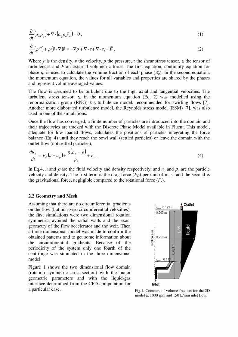
Figure 1 shows the two dimensional flow domain

(rotation symmetric cross-section) with the major

geometric parameters and with the liquid-gas

interface determined from the CFD computation for

a particular case. Fig.1. Contours of volume fraction for the 2D

model at 1000 rpm and 150 L/min inlet flow.

3. Results

3.1. Gas-Liquid interface

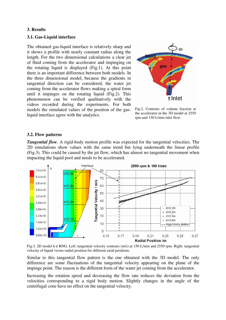
The obtained gas-liquid interface is relatively sharp and

it shows a profile with nearly constant radius along the

length. For the two dimensional calculations a clear jet

of fluid coming from the accelerator and impinging on

the rotating liquid is displayed (Fig.1). At this point

there is an important difference between both models. In

the three dimensional model, because the gradients in

tangential direction can be considered, the water jet

coming from the accelerator flows making a spiral form

until it impinges on the rotating liquid (Fig.2). This

phenomenon can be verified qualitatively with the

videos recorded during the experiments. For both

models the simulated values of the position of the gas-

liquid interface agree with the analytics.

Fig.2. Contours of volume fraction at

the accelerator in the 3D model at 2550

rpm and 150 L/min inlet flow.

3.2. Flow patterns

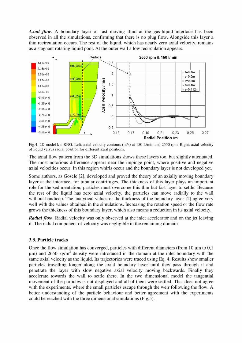
Tangential flow. A rigid-body motion profile was expected for the tangential velocities. The

2D simulations show values with the same trend but lying underneath the linear profile

(Fig.3). This could be caused by the jet flow, which has almost no tangential movement when

impacting the liquid pool and needs to be accelerated.

Fig.3. 2D model k-ε RNG. Left: tangential velocity contours (m/s) at 150 L/min and 2550 rpm. Right: tangential

velocity of liquid versus radial position for different axial positions.

Similar to this tangential flow pattern is the one obtained with the 3D model. The only

difference are some fluctuations of the tangential velocity appearing on the plane of the

impinge point. The reason is the different form of the water jet coming from the accelerator.

Increasing the rotation speed and decreasing the flow rate reduces the deviation from the

velocities corresponding to a rigid body motion. Slightly changes in the angle of the

centrifugal cone have no effect on the tangential velocity.

Axial flow. A boundary layer of fast moving fluid at the gas-liquid interface has been

observed in all the simulations, confirming that there is no plug flow. Alongside this layer a

thin recirculation occurs. The rest of the liquid, which has nearly zero axial velocity, remains

as a stagnant rotating liquid pool. At the outer wall a low recirculation appears.

Fig.4. 2D model k-ε RNG. Left: axial velocity contours (m/s) at 150 L/min and 2550 rpm. Right: axial velocity

of liquid versus radial position for different axial positions.

The axial flow pattern from the 3D simulations shows these layers too, but slightly attenuated.

The most notorious difference appears near the impinge point, where positive and negative

axial velocities occur. In this region whirls occur and the boundary layer is not developed yet.

Some authors, as Gösele [2], developed and proved the theory of an axially moving boundary

layer at the interface, for tubular centrifuges. The thickness of this layer plays an important

role for the sedimentation, particles must overcome this thin but fast layer to settle. Because

the rest of the liquid has zero axial velocity, the particles can move radially to the wall

without handicap. The analytical values of the thickness of the boundary layer [2] agree very

well with the values obtained in the simulations. Increasing the rotation speed or the flow rate

grows the thickness of this boundary layer, which also means a reduction in its axial velocity.

Radial flow. Radial velocity was only observed at the inlet accelerator and on the jet leaving

it. The radial component of velocity was negligible in the remaining domain.

3.3. Particle tracks

Once the flow simulation has converged, particles with different diameters (from 10 µm to 0,1

µm) and 2650 kg/m3 density were introduced in the domain at the inlet boundary with the

same axial velocity as the liquid. Its trajectories were traced using Eq. 4. Results show smaller

particles travelling longer along the axial boundary layer until they pass through it and

penetrate the layer with slow negative axial velocity moving backwards. Finally they

accelerate towards the wall to settle there. In the two dimensional model the tangential

movement of the particles is not displayed and all of them were settled. That does not agree

with the experiments, where the small particles escape through the weir following the flow. A

better understanding of the particle behaviour and better agreement with the experiments

could be reached with the three dimensional simulations (Fig.5).

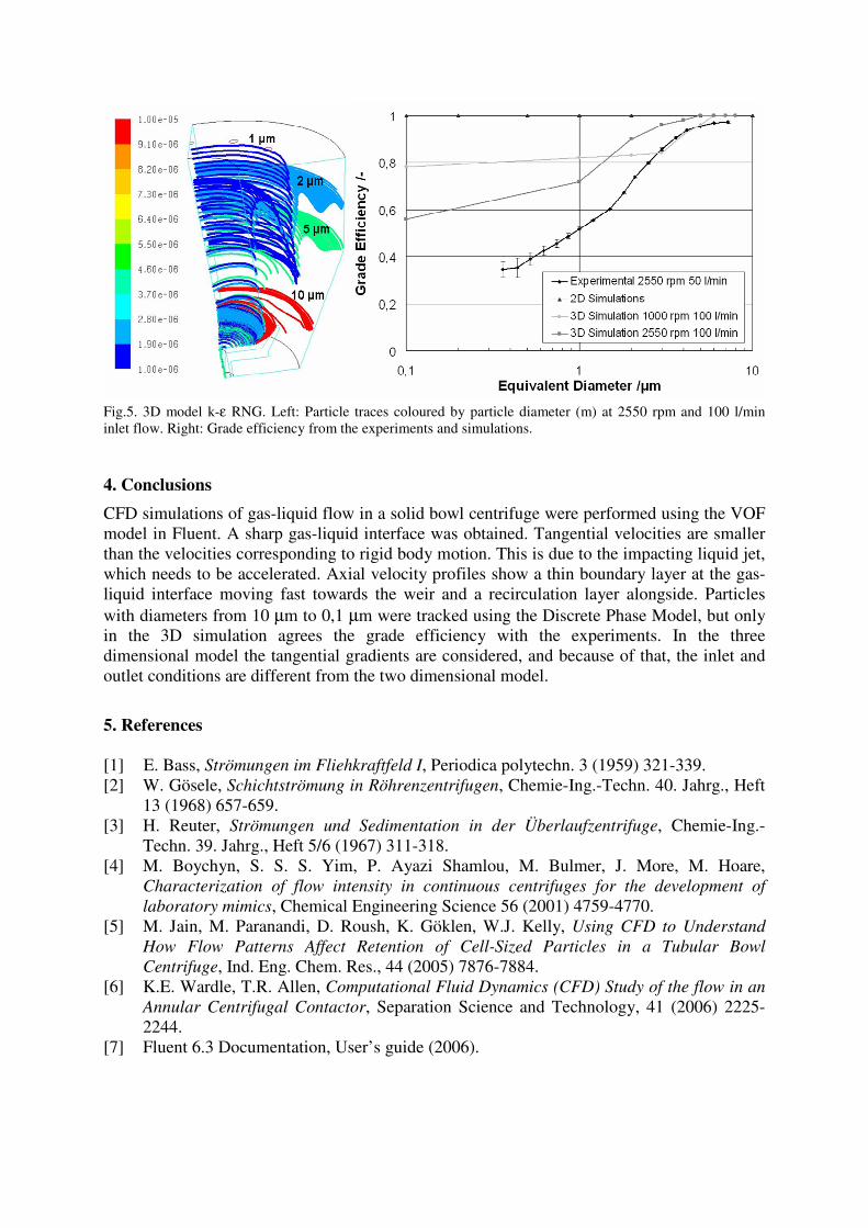
Fig.5. 3D model k-ε RNG. Left: Particle traces coloured by particle diameter (m) at 2550 rpm and 100 l/min

inlet flow. Right: Grade efficiency from the experiments and simulations.

4. Conclusions

CFD simulations of gas-liquid flow in a solid bowl centrifuge were performed using the VOF

model in Fluent. A sharp gas-liquid interface was obtained. Tangential velocities are smaller

than the velocities corresponding to rigid body motion. This is due to the impacting liquid jet,

which needs to be accelerated. Axial velocity profiles show a thin boundary layer at the gas-

liquid interface moving fast towards the weir and a recirculation layer alongside. Particles

with diameters from 10 µm to 0,1 µm were tracked using the Discrete Phase Model, but only

in the 3D simulation agrees the grade efficiency with the experiments. In the three

dimensional model the tangential gradients are considered, and because of that, the inlet and

outlet conditions are different from the two dimensional model.

5. References

[1] E. Bass, Strömungen im Fliehkraftfeld I, Periodica polytechn. 3 (1959) 321-339.

[2] W. Gösele, Schichtströmung in Röhrenzentrifugen, Chemie-Ing.-Techn. 40. Jahrg., Heft

13 (1968) 657-659.

[3] H. Reuter, Strömungen und Sedimentation in der Überlaufzentrifuge, Chemie-Ing.-

Techn. 39. Jahrg., Heft 5/6 (1967) 311-318.

[4] M. Boychyn, S. S. S. Yim, P. Ayazi Shamlou, M. Bulmer, J. More, M. Hoare,

Characterization of flow intensity in continuous centrifuges for the development of laboratory mimics, Chemical Engineering Science 56 (2001) 4759-4770.

[5] M. Jain, M. Paranandi, D. Roush, K. Göklen, W.J. Kelly, Using CFD to Understand How Flow Patterns Affect Retention of Cell-Sized Particles in a Tubular Bowl Centrifuge, Ind. Eng. Chem. Res., 44 (2005) 7876-7884.

[6] K.E. Wardle, T.R. Allen, Computational Fluid Dynamics (CFD) Study of the flow in an Annular Centrifugal Contactor, Separation Science and Technology, 41 (2006) 2225-

2244.

[7] Fluent 6.3 Documentation, User’s guide (2006).