Embed Size (px)
Citation preview
CFD Simulation Methodology for Ground-Coupled Ventilation System
A comparison of alternative modeling strategies using computational fluid dynamics
Jamal K. Alghamdi
Thesis submitted to the faculty of the Virginia Polytechnic Institute and State University in partial fulfillment of the requirements for the degree of
Master of Science
In Architecture
Prof. James Jones, Committee Chair
Prof. Robert Schubert
Prof. Pavlos Vlachos
6/25/2008
Blacksburg, Virginia
Keywords: CFD, GCV, Ground-Coupled Ventilation, Computational Fluid Dynamics, heat exchange, soil temperature, geothermal energy
CFD Simulation Methodology for Ground-Coupled Ventilation System
A comparison of alternative modeling strategies using computational fluid dynamics
Jamal K. Alghamdi
Abstract In the past two decades, a growing interest in alternative energy resources as a
replacement to the non-renewable resources used now days. These alternatives include
geothermal energy which can be used to generate power and reduce the demands on
energy used to heat and cool buildings. Ground-coupled ventilation system is one of the
many applications of the geothermal energy that have a lot of attention in the early 80’s
and 90’s but all designs of the system where based on single case situations. On the other
hand, computational fluid dynamics tools are used to simulate heat and fluid flow in any
real life situation. They start to develop rapidly with the fast development of computers
and processors. These tools provide a great opportunity to simulate and predict the
outcome of most problems with minimum loss and better way to develop new designs.
By using these CFD tools in GCV systems designing procedure, energy can be conserved
and designs going to be improved.
The main objective of this study is to find and develop a CFD modeling strategy
for GCV systems. To accomplish this objective, a case study must be selected, a proper
CFD tool chosen, modeling and meshing method determined, and finally running
simulations and analyzing results. All factors that affect the performance of GCV should
be taken under consideration in that process such as soil, backfill, and pipes thermal
properties. Multiple methods of simulation were proposed and compared to determine the
best modeling approach.
iii Contents
Contents
Abstract .......................................................................................................................... ii
Contents ......................................................................................................................... iii
List of figures .................................................................................................................. v
List of Tables: ............................................................................................................... vii
1. Chapter one: Introduction ........................................................................................ 1
1.1 Background knowledge: .................................................................................... 1
1.2 Heat transfer fundamentals: ............................................................................... 2
1.3 Research focus: ................................................................................................. 4
1.4 Hypothesis: ....................................................................................................... 5
1.5 Research Goal and Objectives: .......................................................................... 5
2. Chapter two: Methodology ...................................................................................... 6
2.1 Experimental: .................................................................................................... 6
2.1.1 Identify an as-built GCV system(s) that would most conveniently support
the research objectives: ............................................................................................ 6
2.1.2 Data monitoring equipments installation: ................................................... 9
2.1.3 Soil sample analysis and determination of thermal properties: .................. 12
2.1.4 Temperature samples selection: ................................................................ 13
2.2 CFD simulations: ............................................................................................ 13
2.2.1 Available CFD tools and their characteristics: .......................................... 13
2.2.2 Test the chosen CFD software: ................................................................. 15
2.2.3 Set a Soil Simulation Model ..................................................................... 16
2.2.4 Setup a base CFD model for the selected GCV system ............................. 17
2.3 Data analysis: .................................................................................................. 30
iv
3. Chapter three: Results ............................................................................................ 31
3.1 Experimental site monitoring and comparisons results .................................... 31
3.2 CFD tools comparative investigation results .................................................... 33
3.3 CFD software testing results ........................................................................... 34
3.4 Soil sample simulation results ......................................................................... 34
3.5 GCV system modeling methods simulation results .......................................... 36
3.6 Data analysis results ........................................................................................ 43
3.7 Multiple pipes simulation: ............................................................................... 43
4. Chapter Four: Conclusions .................................................................................... 45
Works Cited .................................................................................................................. 46
v List of figures
List of figures
Figure 1-1: Schematic image of GCV system -------------------------------------------------- 1
Figure 1-2: GCV system environment and design factors ------------------------------------ 2
Figure 1-3: Soil temperature distribution as factor of depth (DOE & Tech, 2004) -------- 3
Figure 1-4: Schematic heat flow conditions within a GCV system -------------------------- 3
Figure 1-5: Issues to be covered in this research ----------------------------------------------- 4
Figure 2-1: Solar House CM after it’s been constructed in 1981 ---------------------------- 7
Figure 2-2: Vitrified clay pipes used in the Solar House CM’s GCV system and the
gravel backfill -------------------------------------------------------------------------------------- 7
Figure 2-3: Schematic drawing of the Solar House CM ground coupled system ---------- 8
Figure 2-4: 3D shows pipes numbering and the air flow assigned to each one ------------- 9
Figure 2-5: Air flow control via fans with dampers ------------------------------------------ 10
Figure 2-6: Thermocouple located at the inlet of the pipe (right) and the buried below
grade (left) ----------------------------------------------------------------------------------------- 10
Figure 2-7: Datalogger setup at site ------------------------------------------------------------ 11
Figure 2-8: Thermocouples locations in pipe number 4 -------------------------------------- 11
Figure 2-9: Soil samples taken from the site -------------------------------------------------- 12
Figure 2-10: The internal flow through parallel plates --------------------------------------- 15
Figure 2-11: Soil model with probe location in the CFD ------------------------------------ 16
Figure 2-12: Single pipe set with dimensions ------------------------------------------------- 17
Figure 2-13: Four pipes set model with dimensions ------------------------------------------ 17
Figure 2-14: Regions and surfaces classified in the problem model ------------------------ 18
Figure 2-15: Generated mesh for the problem surface and volume ------------------------- 19
Figure 2-16: Inflation layers defined within surface mesh ----------------------------------- 19
Figure 2-17: Soil domain faces locations ------------------------------------------------------ 21
Figure 2-18: Solver software during simulation process ------------------------------------- 29
Figure 2-19: Results visualization in post-process -------------------------------------------- 30
Figure 3-1: Relationship between air volume and temperature change -------------------- 31
Figure 3-2: 24 Hours period temperature change (10/08/2007) ----------------------------- 32
vi List of figures
Figure 3-3: 24 Hours period temperature change (01/21/2008) ----------------------------- 32
Figure 3-4: Final results of both analytical and CFD simulation to the internal flow
problem -------------------------------------------------------------------------------------------- 34
Figure 3-5: Relationship between site soil temperature and simulation output temperature
------------------------------------------------------------------------------------------------------ 36
Figure 3-6: Method no. 1 (air turbulence) ----------------------------------------------------- 37
Figure 3-7: Method no. 2 (air turbulence) ----------------------------------------------------- 37
Figure 3-8: Method no. 3 (pipe wall roughness) ---------------------------------------------- 38
Figure 3-9: Method no. 4 (pipe wall roughness) ---------------------------------------------- 38
Figure 3-10: Method no. 5 (Backfill thickness) ----------------------------------------------- 39
Figure 3-11: Method no. 6 (Backfill thickness) ----------------------------------------------- 39
Figure 3-12: Method no. 7 (Backfill thickness) ----------------------------------------------- 40
Figure 3-13: Method no. 8 (boundary condition) --------------------------------------------- 40
Figure 3-14: Method no. 9 (boundary condition) --------------------------------------------- 41
Figure 3-15: Method no. 10 (boundary condition) -------------------------------------------- 41
Figure 3-16: Method no. 11 (boundary condition) -------------------------------------------- 42
Figure 3-17: Method no. 12 (mixed) ----------------------------------------------------------- 42
Figure 3-18: Data outcome of multiple pipes simulation ------------------------------------ 44
vii List of Tables:
List of Tables:
Table 2-1: Temperature samples chosen for the CFD simulation from the monitored
experiment site ------------------------------------------------------------------------------------ 13
Table 2-2: Parameters of the problem ---------------------------------------------------------- 15
Table 2-3: Materials thermal properties -------------------------------------------------------- 20
Table 2-4: Air domain boundary conditions definitions ------------------------------------- 21
Table 2-5: Pipes domain boundary conditions definitions ----------------------------------- 21
Table 2-6: Backfill domain boundary conditions definitions -------------------------------- 21
Table 2-7: Soil domain boundary conditions definitions------------------------------------- 21
Table 2-8: List of the 12 simulation methods used in this research and their properties - 22
Table 2-9: Method No. 1 (air turbulence) ------------------------------------------------------ 23
Table 2-10: Method No. 2 (air turbulence) ---------------------------------------------------- 23
Table 2-11: Method No. 3 (pipe wall roughness) --------------------------------------------- 24
Table 2-12: Method No. 4 (pipe wall roughness) --------------------------------------------- 24
Table 2-13: Method No. 5 (backfill thickness) ------------------------------------------------ 25
Table 2-14: Method No. 6 (backfill thickness) ------------------------------------------------ 25
Table 2-15: Method No. 7 (backfill thickness) ------------------------------------------------ 26
Table 2-16: Method No. 8 (soil boundary condition) ---------------------------------------- 26
Table 2-17: Method No. 9 (soil boundary condition) ---------------------------------------- 27
Table 2-18: Method No. 10 (soil boundary condition) --------------------------------------- 27
Table 2-19: Method No. 11 (soil boundary condition) --------------------------------------- 28
Table 2-20: Method No. 12 (Mixed) ----------------------------------------------------------- 28
Table 3-1: CFD software comparisons --------------------------------------------------------- 33
Table 3-2: Results of stage one in soil simulation (in F°) ------------------------------------ 35
Table 3-3: Results of stage two of soil simulation (F°) -------------------------------------- 35
Table 3-4: Method no. 1 (air turbulence) ------------------------------------------------------ 36
Table 3-5: Method no. 2 (air turbulence) ------------------------------------------------------ 37
Table 3-6: Method no. 3 (pipe wall roughness) ----------------------------------------------- 38
Table 3-7: Method no. 4 (pipe wall roughness) ----------------------------------------------- 38
viii List of Tables:
Table 3-8: Method no. 5 (Backfill thickness) ------------------------------------------------- 39
Table 3-9: Method no. 6 (Backfill thickness) ------------------------------------------------- 39
Table 3-10: Method no. 7 (Backfill thickness) ------------------------------------------------ 40
Table 3-11: Method no. 8 (boundary condition) ---------------------------------------------- 40
Table 3-12: Method no. 9 (boundary condition) ---------------------------------------------- 41
Table 3-13: Method no. 10 (boundary condition) --------------------------------------------- 41
Table 3-14: Method no. 11 (boundary condition) --------------------------------------------- 42
Table 3-15: Method no. 12 (mixed) ------------------------------------------------------------ 42
Table 3-16: Simulation data statistical comparison results via Fisher’s LSD means
comparison method ------------------------------------------------------------------------------- 43
Table 3-17: Multiple pipes simulation run results -------------------------------------------- 44
1 Chapter one: Introduction
1. Chapter one: Introduction
1.1 Background knowledge:
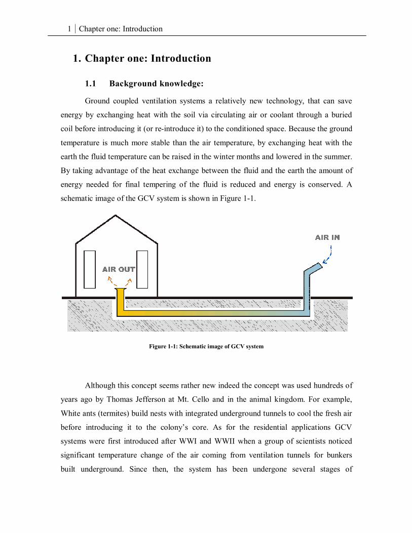
Ground coupled ventilation systems a relatively new technology, that can save
energy by exchanging heat with the soil via circulating air or coolant through a buried
coil before introducing it (or re-introduce it) to the conditioned space. Because the ground
temperature is much more stable than the air temperature, by exchanging heat with the
earth the fluid temperature can be raised in the winter months and lowered in the summer.
By taking advantage of the heat exchange between the fluid and the earth the amount of
energy needed for final tempering of the fluid is reduced and energy is conserved. A
schematic image of the GCV system is shown in Figure 1-1.
Figure 1-1: Schematic image of GCV system
Although this concept seems rather new indeed the concept was used hundreds of
years ago by Thomas Jefferson at Mt. Cello and in the animal kingdom. For example,
White ants (termites) build nests with integrated underground tunnels to cool the fresh air
before introducing it to the colony’s core. As for the residential applications GCV
systems were first introduced after WWI and WWII when a group of scientists noticed
significant temperature change of the air coming from ventilation tunnels for bunkers
built underground. Since then, the system has been undergone several stages of
2 Chapter one: Introduction
development which led to the invention of the geothermal heat exchange system that uses
water rather than soil as the mediate. Many materials and methods of exchange have been
investigated over the past several years but the two most common types are the closed
loop system and open loop system. The closed loop circulates air through a heat pump.
This system typically has lower efficiency than the open loop system that uses outdoor air
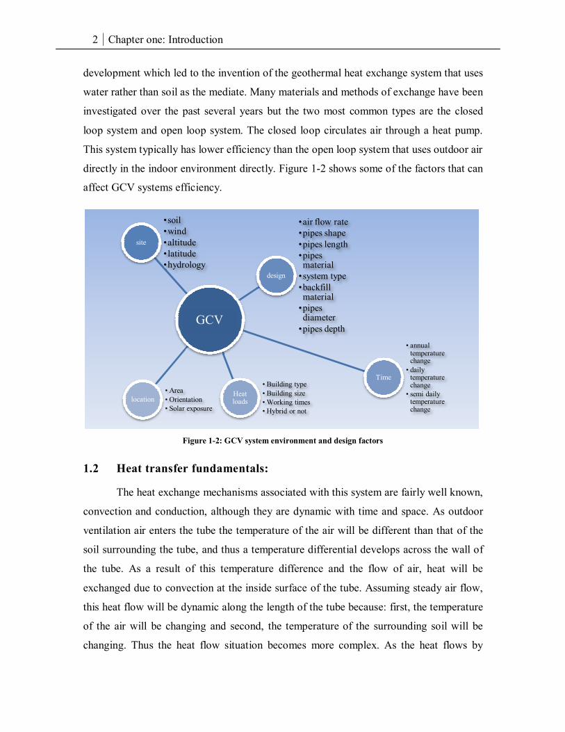
directly in the indoor environment directly. Figure 1-2 shows some of the factors that can
affect GCV systems efficiency.
Figure 1-2: GCV system environment and design factors
1.2 Heat transfer fundamentals:
The heat exchange mechanisms associated with this system are fairly well known,
convection and conduction, although they are dynamic with time and space. As outdoor
ventilation air enters the tube the temperature of the air will be different than that of the
soil surrounding the tube, and thus a temperature differential develops across the wall of
the tube. As a result of this temperature difference and the flow of air, heat will be
exchanged due to convection at the inside surface of the tube. Assuming steady air flow,
this heat flow will be dynamic along the length of the tube because: first, the temperature
of the air will be changing and second, the temperature of the surrounding soil will be
changing. Thus the heat flow situation becomes more complex. As the heat flows by
site
•soil•wind•altitude• latitude•hydrology
design
•air flow rate•pipes shape•pipes length•pipes material
•system type•backfill material
•pipes diameter
•pipes depth
Time
• annual temperature change
• daily temperature change
• semi daily temperature change
Heat loads
• Building type• Building size• Working times• Hybrid or not
location• Area• Orientation• Solar exposure
GCV
3 Chapter one: Introduction
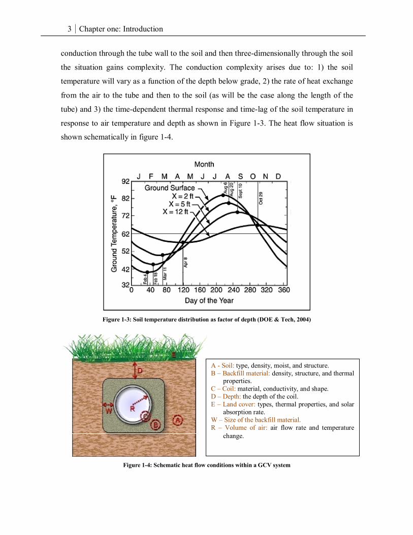
conduction through the tube wall to the soil and then three-dimensionally through the soil
the situation gains complexity. The conduction complexity arises due to: 1) the soil
temperature will vary as a function of the depth below grade, 2) the rate of heat exchange
from the air to the tube and then to the soil (as will be the case along the length of the
tube) and 3) the time-dependent thermal response and time-lag of the soil temperature in
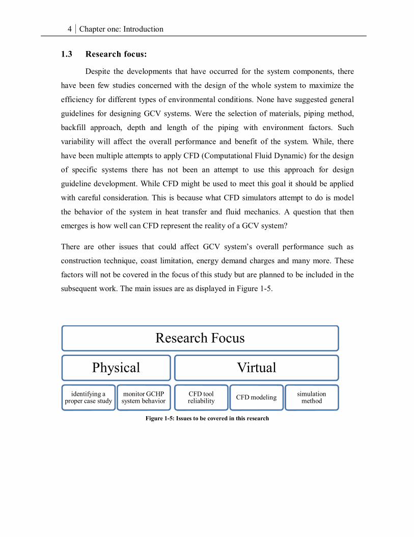
response to air temperature and depth as shown in Figure 1-3. The heat flow situation is
shown schematically in figure 1-4.
Figure 1-3: Soil temperature distribution as factor of depth (DOE & Tech, 2004)
Figure 1-4: Schematic heat flow conditions within a GCV system
A - Soil: type, density, moist, and structure. B – Backfill material: density, structure, and thermal
properties. C – Coil: material, conductivity, and shape. D – Depth: the depth of the coil. E – Land cover: types, thermal properties, and solar
absorption rate. W – Size of the backfill material. R – Volume of air: air flow rate and temperature
change.
4 Chapter one: Introduction
1.3 Research focus:
Despite the developments that have occurred for the system components, there
have been few studies concerned with the design of the whole system to maximize the
efficiency for different types of environmental conditions. None have suggested general
guidelines for designing GCV systems. Were the selection of materials, piping method,
backfill approach, depth and length of the piping with environment factors. Such
variability will affect the overall performance and benefit of the system. While, there
have been multiple attempts to apply CFD (Computational Fluid Dynamic) for the design
of specific systems there has not been an attempt to use this approach for design
guideline development. While CFD might be used to meet this goal it should be applied
with careful consideration. This is because what CFD simulators attempt to do is model
the behavior of the system in heat transfer and fluid mechanics. A question that then
emerges is how well can CFD represent the reality of a GCV system?
There are other issues that could affect GCV system’s overall performance such as
construction technique, coast limitation, energy demand charges and many more. These
factors will not be covered in the focus of this study but are planned to be included in the
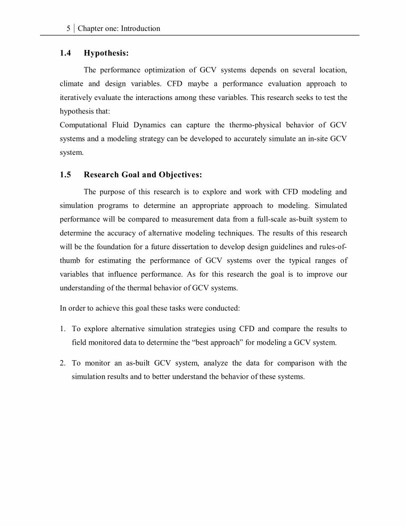
subsequent work. The main issues are as displayed in Figure 1-5.
Figure 1-5: Issues to be covered in this research
Research Focus
Physical
identifying a proper case study
monitor GCHP system behavior
Virtual
CFD tool reliability CFD modeling simulation
method
5 Chapter one: Introduction
1.4 Hypothesis:
The performance optimization of GCV systems depends on several location,
climate and design variables. CFD maybe a performance evaluation approach to
iteratively evaluate the interactions among these variables. This research seeks to test the
hypothesis that:
Computational Fluid Dynamics can capture the thermo-physical behavior of GCV
systems and a modeling strategy can be developed to accurately simulate an in-site GCV
system.
1.5 Research Goal and Objectives:
The purpose of this research is to explore and work with CFD modeling and
simulation programs to determine an appropriate approach to modeling. Simulated
performance will be compared to measurement data from a full-scale as-built system to
determine the accuracy of alternative modeling techniques. The results of this research
will be the foundation for a future dissertation to develop design guidelines and rules-of-
thumb for estimating the performance of GCV systems over the typical ranges of
variables that influence performance. As for this research the goal is to improve our
understanding of the thermal behavior of GCV systems.
In order to achieve this goal these tasks were conducted:
1. To explore alternative simulation strategies using CFD and compare the results to
field monitored data to determine the “best approach” for modeling a GCV system.
2. To monitor an as-built GCV system, analyze the data for comparison with the
simulation results and to better understand the behavior of these systems.
6 Chapter two: Methodology
2. Chapter two: Methodology To test the research hypothesis with a CFD tool there must be a reference point to
compare simulation result to it and find the proper method of simulation. This reference
could be hypothetical or experimental. Hypothetical reference has the mathematical and
physical laws to support it but it may not include all factors affecting the GCV system
performance and cause a data bias. On the other hand, experimental monitoring will
provide the research with the full spectrum plus it gives an opportunity to study the
behavior of the GCV system during the monitoring period.
Research methodology described in this chapter will be under three phases:
Experimental, CFD simulations, and data analysis.
2.1 Experimental:
2.1.1 Identify an as-built GCV system(s) that would most conveniently
support the research objectives:
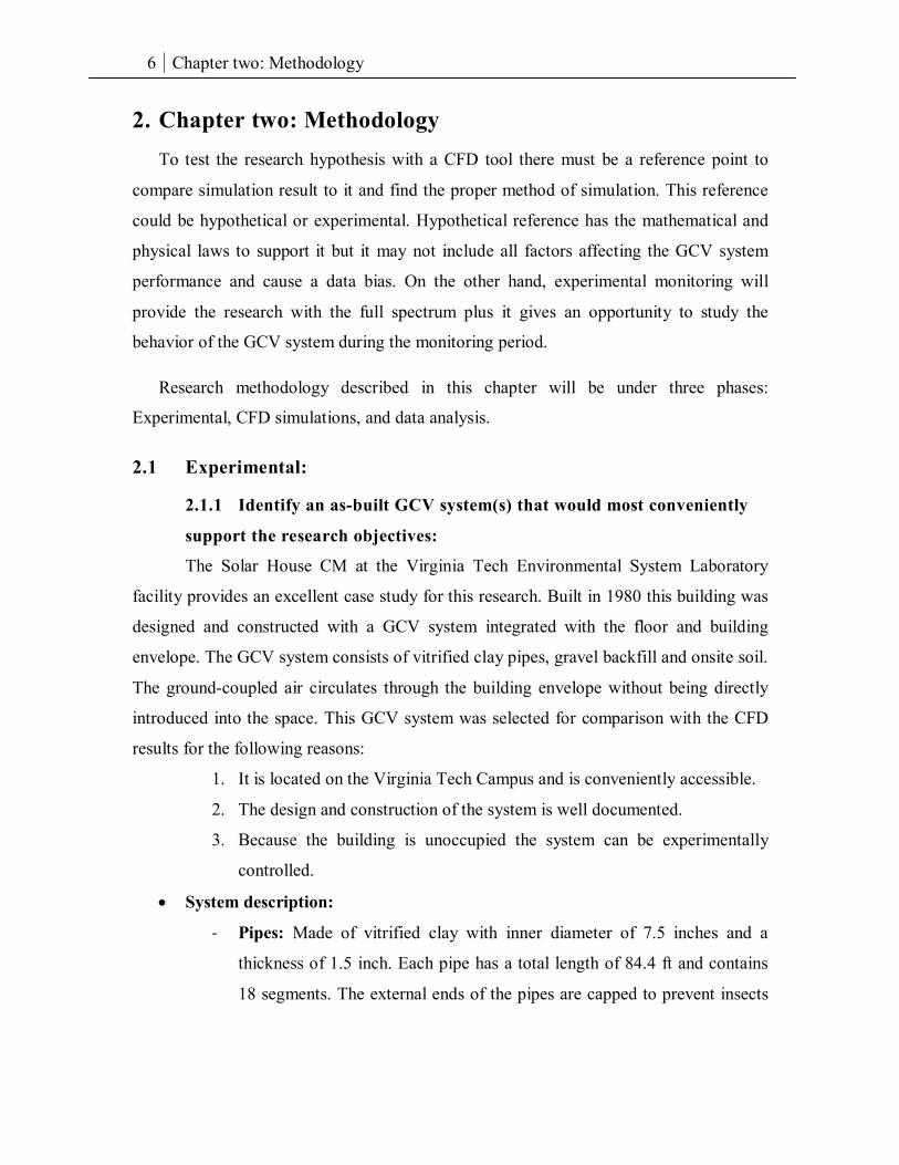
The Solar House CM at the Virginia Tech Environmental System Laboratory
facility provides an excellent case study for this research. Built in 1980 this building was
designed and constructed with a GCV system integrated with the floor and building
envelope. The GCV system consists of vitrified clay pipes, gravel backfill and onsite soil.
The ground-coupled air circulates through the building envelope without being directly
introduced into the space. This GCV system was selected for comparison with the CFD
results for the following reasons:
1. It is located on the Virginia Tech Campus and is conveniently accessible.
2. The design and construction of the system is well documented.
3. Because the building is unoccupied the system can be experimentally
controlled.
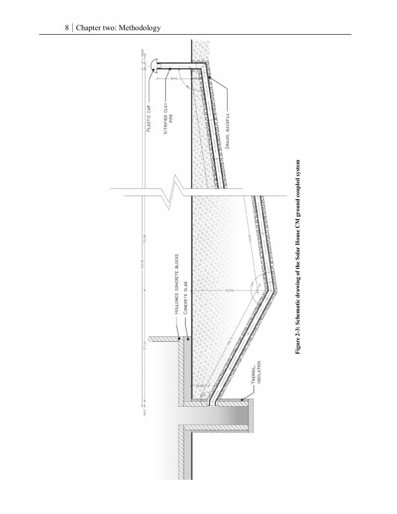
• System description:
- Pipes: Made of vitrified clay with inner diameter of 7.5 inches and a
thickness of 1.5 inch. Each pipe has a total length of 84.4 ft and contains
18 segments. The external ends of the pipes are capped to prevent insects
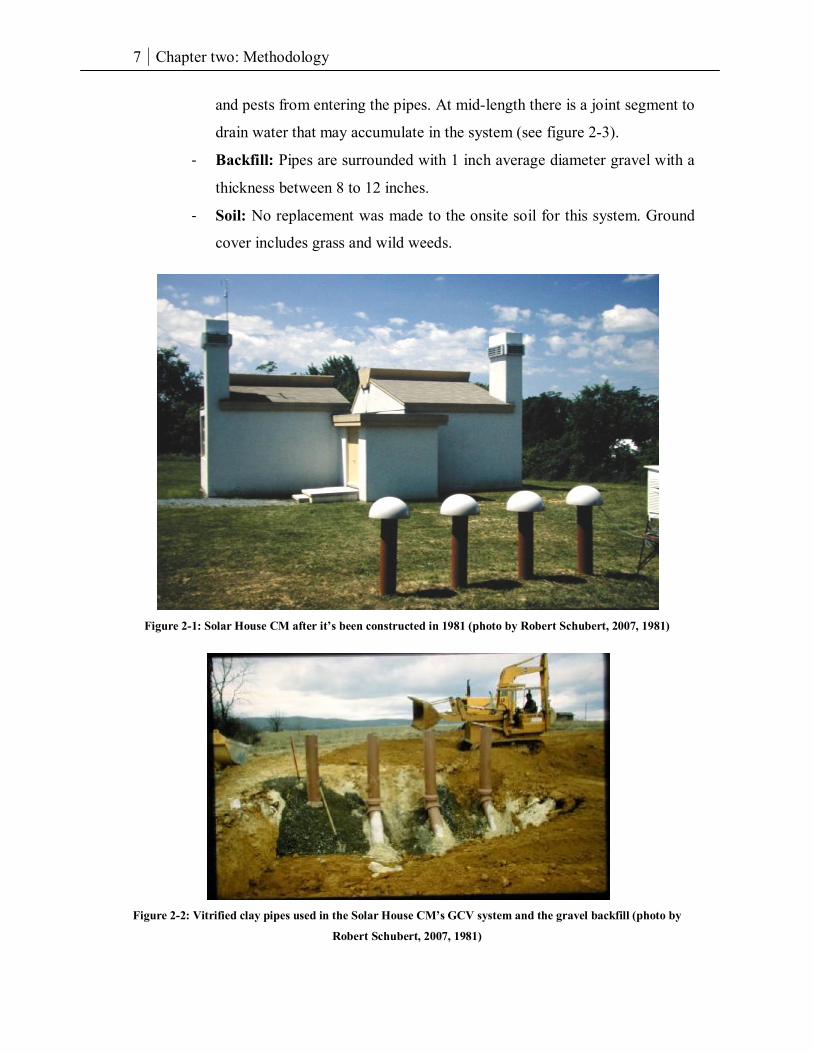
7 Chapter two: Methodology
and pests from entering the pipes. At mid-length there is a joint segment to
drain water that may accumulate in the system (see figure 2-3).
- Backfill: Pipes are surrounded with 1 inch average diameter gravel with a
thickness between 8 to 12 inches.
- Soil: No replacement was made to the onsite soil for this system. Ground
cover includes grass and wild weeds.
Figure 2-1: Solar House CM after it’s been constructed in 1981 (photo by Robert Schubert, 2007, 1981)
Figure 2-2: Vitrified clay pipes used in the Solar House CM’s GCV system and the gravel backfill (photo by
Robert Schubert, 2007, 1981)
8 Chapter two: Methodology
Figu
re 2
-3: S
chem
atic
dra
win
g of
the
Sola
r H
ouse
CM
gro
und
coup
led
syst
em
9 Chapter two: Methodology
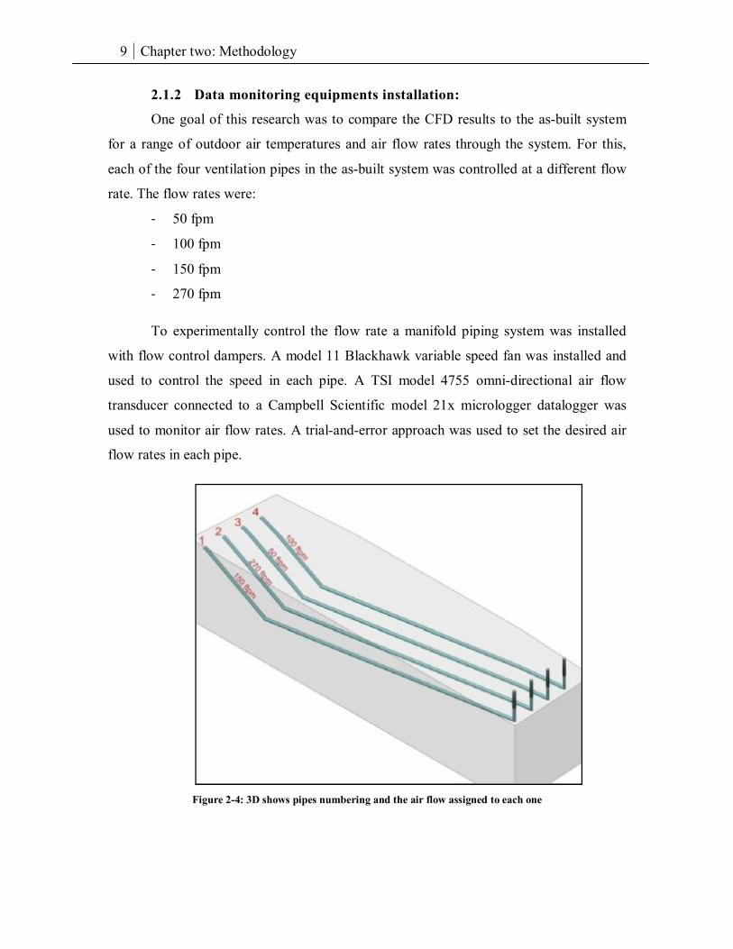
2.1.2 Data monitoring equipments installation:
One goal of this research was to compare the CFD results to the as-built system
for a range of outdoor air temperatures and air flow rates through the system. For this,
each of the four ventilation pipes in the as-built system was controlled at a different flow
rate. The flow rates were:
- 50 fpm
- 100 fpm
- 150 fpm
- 270 fpm
To experimentally control the flow rate a manifold piping system was installed
with flow control dampers. A model 11 Blackhawk variable speed fan was installed and
used to control the speed in each pipe. A TSI model 4755 omni-directional air flow
transducer connected to a Campbell Scientific model 21x micrologger datalogger was
used to monitor air flow rates. A trial-and-error approach was used to set the desired air
flow rates in each pipe.
Figure 2-4: 3D shows pipes numbering and the air flow assigned to each one
10 Chapter two: Methodology
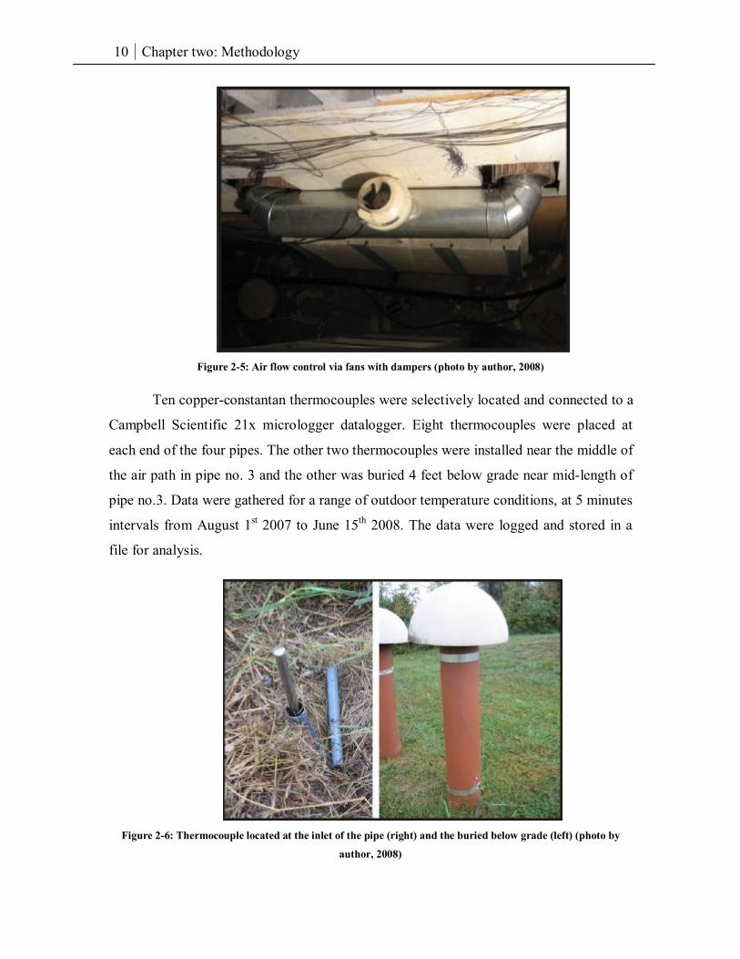
Figure 2-5: Air flow control via fans with dampers (photo by author, 2008)
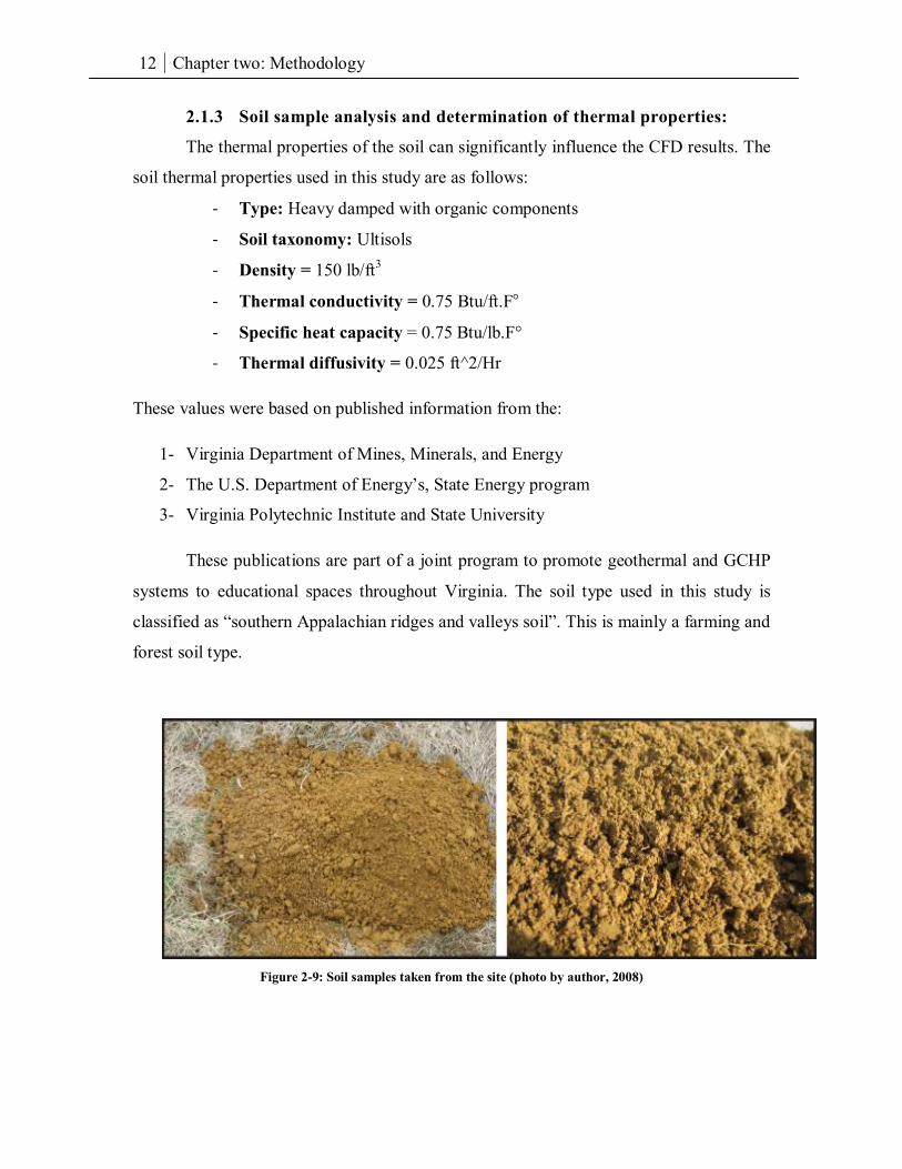
Ten copper-constantan thermocouples were selectively located and connected to a
Campbell Scientific 21x micrologger datalogger. Eight thermocouples were placed at
each end of the four pipes. The other two thermocouples were installed near the middle of
the air path in pipe no. 3 and the other was buried 4 feet below grade near mid-length of
pipe no.3. Data were gathered for a range of outdoor temperature conditions, at 5 minutes
intervals from August 1st 2007 to June 15th 2008. The data were logged and stored in a
file for analysis.
Figure 2-6: Thermocouple located at the inlet of the pipe (right) and the buried below grade (left) (photo by
author, 2008)
11 Chapter two: Methodology
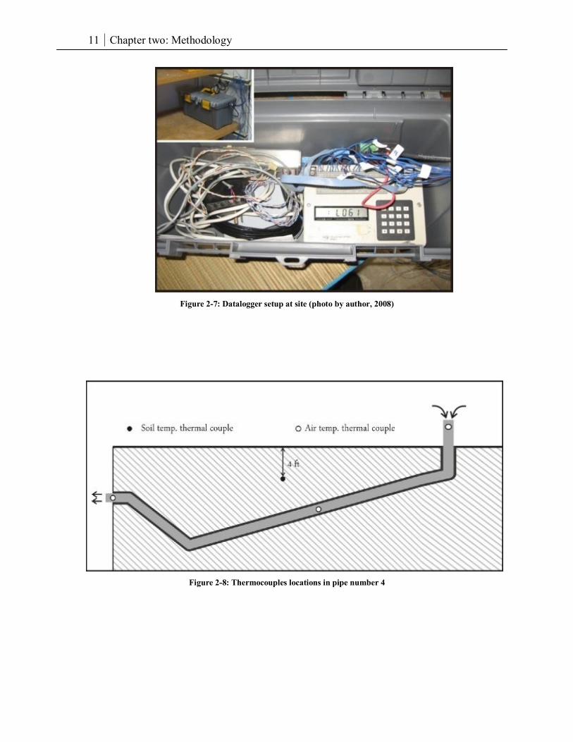
Figure 2-7: Datalogger setup at site (photo by author, 2008)
Figure 2-8: Thermocouples locations in pipe number 4
12 Chapter two: Methodology
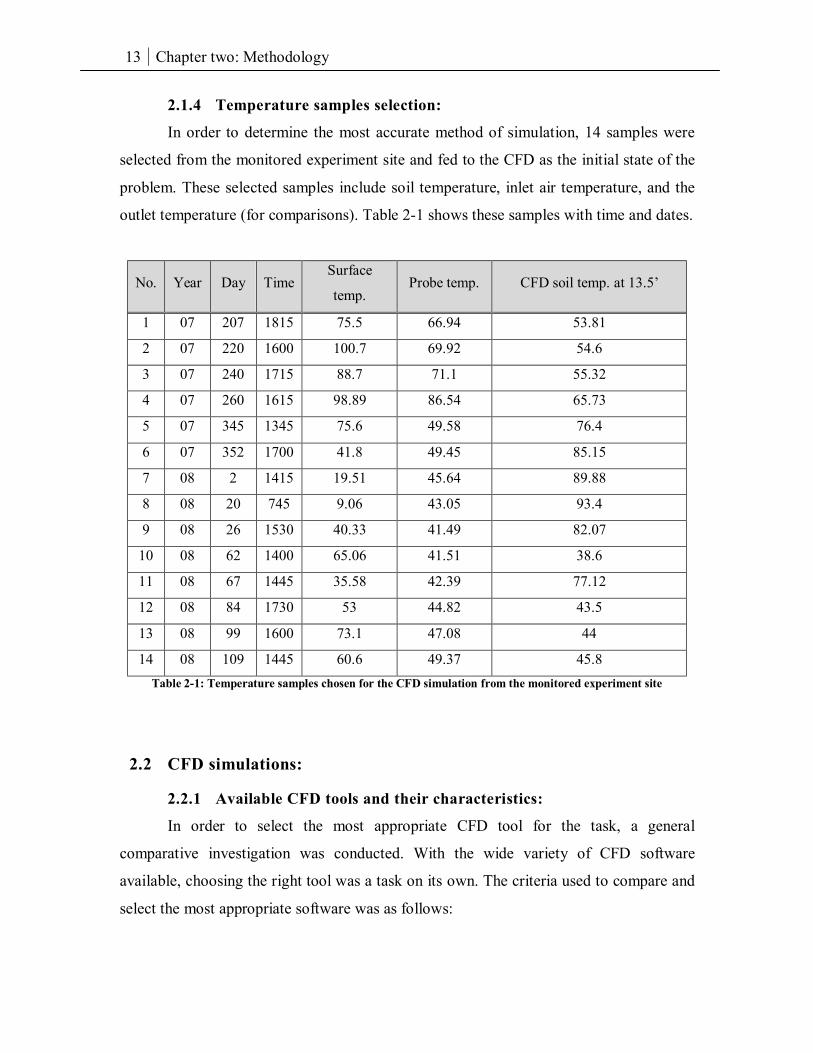
2.1.3 Soil sample analysis and determination of thermal properties:
The thermal properties of the soil can significantly influence the CFD results. The
soil thermal properties used in this study are as follows:
- Type: Heavy damped with organic components
- Soil taxonomy: Ultisols
- Density = 150 lb/ft3
- Thermal conductivity = 0.75 Btu/ft.F°
- Specific heat capacity = 0.75 Btu/lb.F°
- Thermal diffusivity = 0.025 ft^2/Hr
These values were based on published information from the:
1- Virginia Department of Mines, Minerals, and Energy
2- The U.S. Department of Energy’s, State Energy program
3- Virginia Polytechnic Institute and State University
These publications are part of a joint program to promote geothermal and GCHP
systems to educational spaces throughout Virginia. The soil type used in this study is
classified as “southern Appalachian ridges and valleys soil”. This is mainly a farming and
forest soil type.
Figure 2-9: Soil samples taken from the site (photo by author, 2008)
13 Chapter two: Methodology
2.1.4 Temperature samples selection:
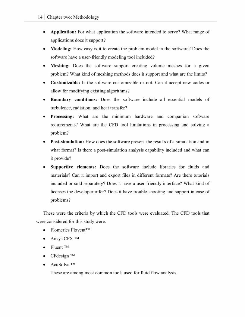
In order to determine the most accurate method of simulation, 14 samples were
selected from the monitored experiment site and fed to the CFD as the initial state of the
problem. These selected samples include soil temperature, inlet air temperature, and the
outlet temperature (for comparisons). Table 2-1 shows these samples with time and dates.
No. Year Day Time Surface
temp. Probe temp. CFD soil temp. at 13.5’
1 07 207 1815 75.5 66.94 53.81
2 07 220 1600 100.7 69.92 54.6
3 07 240 1715 88.7 71.1 55.32
4 07 260 1615 98.89 86.54 65.73
5 07 345 1345 75.6 49.58 76.4
6 07 352 1700 41.8 49.45 85.15
7 08 2 1415 19.51 45.64 89.88
8 08 20 745 9.06 43.05 93.4
9 08 26 1530 40.33 41.49 82.07
10 08 62 1400 65.06 41.51 38.6
11 08 67 1445 35.58 42.39 77.12
12 08 84 1730 53 44.82 43.5
13 08 99 1600 73.1 47.08 44
14 08 109 1445 60.6 49.37 45.8 Table 2-1: Temperature samples chosen for the CFD simulation from the monitored experiment site
2.2 CFD simulations:
2.2.1 Available CFD tools and their characteristics:
In order to select the most appropriate CFD tool for the task, a general
comparative investigation was conducted. With the wide variety of CFD software
available, choosing the right tool was a task on its own. The criteria used to compare and
select the most appropriate software was as follows:
14 Chapter two: Methodology
• Application: For what application the software intended to serve? What range of
applications does it support?
• Modeling: How easy is it to create the problem model in the software? Does the
software have a user-friendly modeling tool included?
• Meshing: Does the software support creating volume meshes for a given
problem? What kind of meshing methods does it support and what are the limits?
• Customizable: Is the software customizable or not. Can it accept new codes or
allow for modifying existing algorithms?
• Boundary conditions: Does the software include all essential models of
turbulence, radiation, and heat transfer?
• Processing: What are the minimum hardware and companion software
requirements? What are the CFD tool limitations in processing and solving a
problem?
• Post-simulation: How does the software present the results of a simulation and in
what format? Is there a post-simulation analysis capability included and what can
it provide?
• Supportive elements: Does the software include libraries for fluids and
materials? Can it import and export files in different formats? Are there tutorials
included or sold separately? Does it have a user-friendly interface? What kind of
licenses the developer offer? Does it have trouble-shooting and support in case of
problems?
These were the criteria by which the CFD tools were evaluated. The CFD tools that
were considered for this study were:
• Flomerics Flovent™
• Ansys CFX ™
• Fluent ™
• CFdesign ™
• AcuSolve ™
These are among most common tools used for fluid flow analysis.
15 Chapter two: Methodology
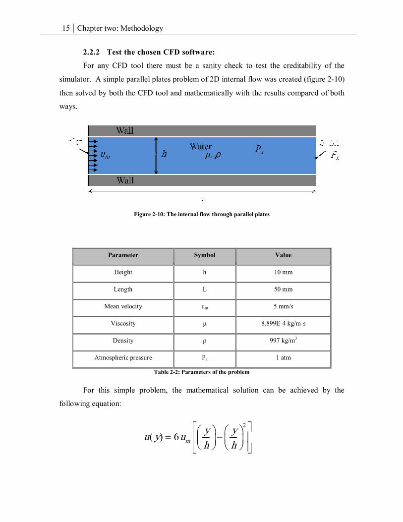
2.2.2 Test the chosen CFD software:
For any CFD tool there must be a sanity check to test the creditability of the
simulator. A simple parallel plates problem of 2D internal flow was created (figure 2-10)
then solved by both the CFD tool and mathematically with the results compared of both
ways.
Figure 2-10: The internal flow through parallel plates
Parameter Symbol Value
Height h 10 mm
Length L 50 mm
Mean velocity um 5 mm/s
Viscosity μ 8.899E-4 kg/m-s
Density ρ 997 kg/m3
Atmospheric pressure Pa 1 atm
Table 2-2: Parameters of the problem
For this simple problem, the mathematical solution can be achieved by the
following equation:
2
( ) 6 my yu y uh h
= −
16 Chapter two: Methodology
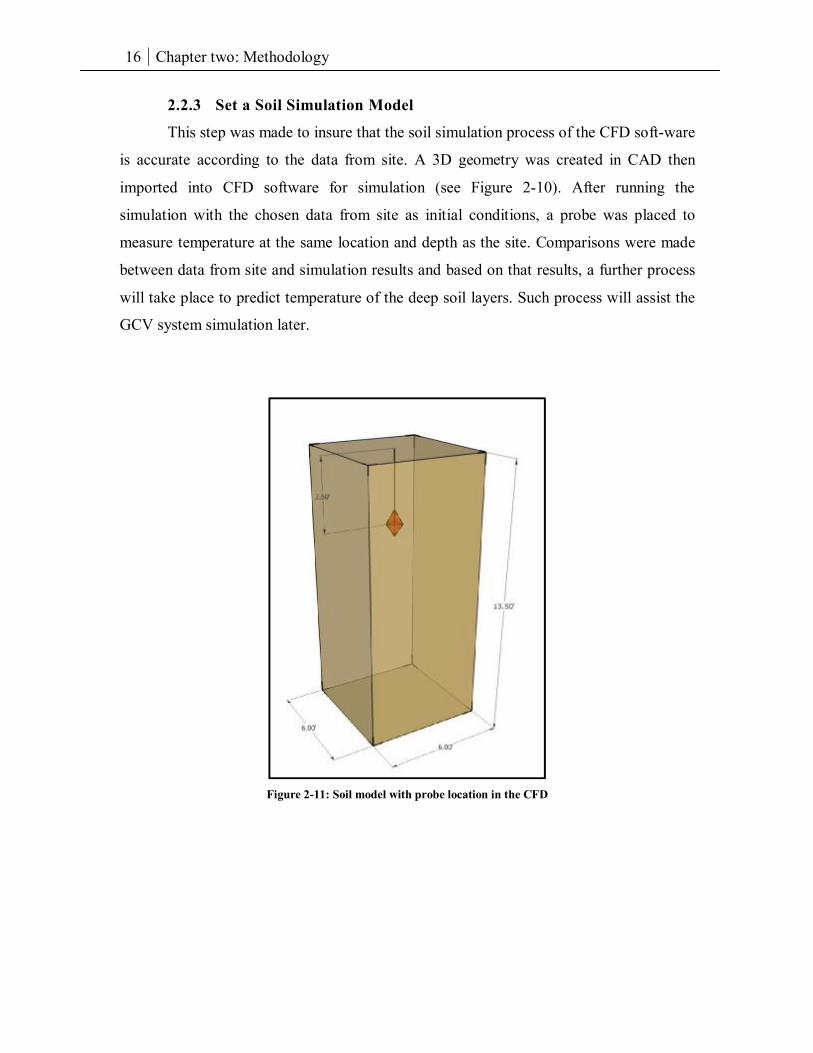
2.2.3 Set a Soil Simulation Model
This step was made to insure that the soil simulation process of the CFD soft-ware
is accurate according to the data from site. A 3D geometry was created in CAD then
imported into CFD software for simulation (see Figure 2-10). After running the
simulation with the chosen data from site as initial conditions, a probe was placed to
measure temperature at the same location and depth as the site. Comparisons were made
between data from site and simulation results and based on that results, a further process
will take place to predict temperature of the deep soil layers. Such process will assist the
GCV system simulation later.
Figure 2-11: Soil model with probe location in the CFD
17 Chapter two: Methodology
2.2.4 Setup a base CFD model for the selected GCV system
Setting a model for the selected GCHP system must go through the following
procedures:
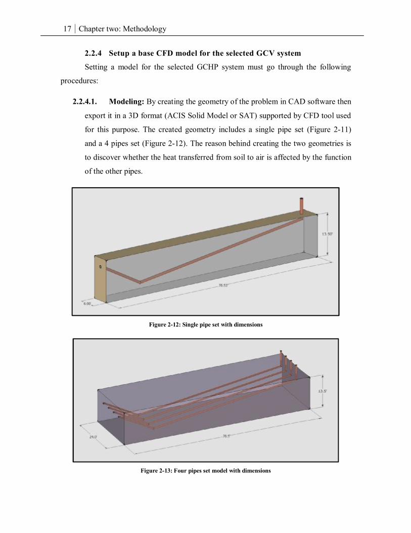
2.2.4.1. Modeling: By creating the geometry of the problem in CAD software then
export it in a 3D format (ACIS Solid Model or SAT) supported by CFD tool used
for this purpose. The created geometry includes a single pipe set (Figure 2-11)
and a 4 pipes set (Figure 2-12). The reason behind creating the two geometries is
to discover whether the heat transferred from soil to air is affected by the function
of the other pipes.
Figure 2-12: Single pipe set with dimensions
Figure 2-13: Four pipes set model with dimensions
18 Chapter two: Methodology
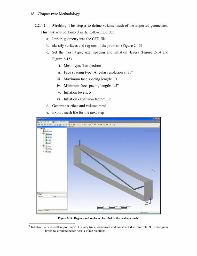
2.2.4.2. Meshing: This step is to define volume mesh of the imported geometries.
This task was performed in the following order:
a. Import geometry into the CFD file
b. classify surfaces and regions of the problem (Figure 2-13)
c. Set the mesh type, size, spacing and inflation1 layers (Figure 2-14 and
Figure 2-15)
i. Mesh type: Tetrahedron
ii. Face spacing type: Angular resolution at 30°
iii. Maximum face spacing length: 10”
iv. Minimum face spacing length: 1.5”
v. Inflation levels: 5
vi. Inflation expansion factor: 1.2
d. Generate surface and volume mesh
e. Export mesh file for the next step
Figure 2-14: Regions and surfaces classified in the problem model
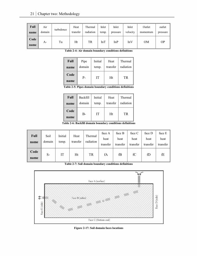
1 Inflation: a near-wall region mesh. Usually finer, structured and constructed in multiple 2D rectangular
levels to simulate better near-surface reactions.
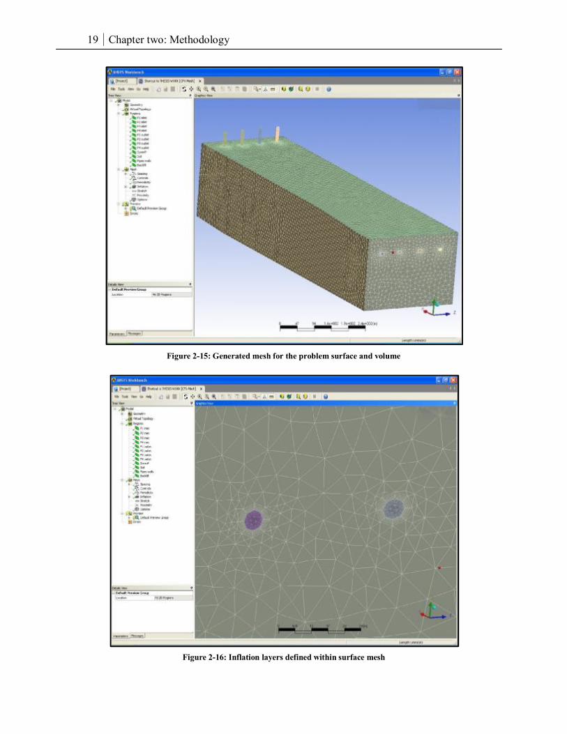
19 Chapter two: Methodology
Figure 2-15: Generated mesh for the problem surface and volume
Figure 2-16: Inflation layers defined within surface mesh

20 Chapter two: Methodology
2.2.4.3. Problem definition: problem definition is the step where elements of the
given geometry are fed into the CFD. These elements such as domains identified,
materials assigned, thermal properties defined, and finally inlets and outlets
locations are located. The values of the defined elements as follows:
a. Domains: Soil (solid), pipe (solid), backfill (solid), and air (fluid)
b. Materials defined: Soil, vitrified clay, gravel, air
c. Materials thermal properties: see table 2-3
material Density Thickness Thermal
conductivity
Thermal
diffusivity
specific heat
capacity
Soil 150 lb/ft3 --- 0.75 Btu/Ft.F° 0.025 Ft2/Hr 0.23 Btu/lb.F°
Vitrified clay 2000kg/m3 1.5” 1.2 W/m*K 0.023 Ft2/Hr 0.215 Btu/lb.F°
Air (at 25° c) Default --- Default Default Default
Gravel 2629 kg/m3 3” – 5” (1”) 4.8 W/m*K --- 0.79 kJ/(kg K)
Table 2-3: Materials thermal properties
2.2.4.4. Boundary conditions: boundary conditions and initial state are set to
insure proper thermal behavior that matches the existed GCV system (Figure 2-
15). Furthermore, these conditions are the main variables in this research and by
tuning them the results will vary. The process of defining the initial boundary
conditions includes:
a. Air domain boundary conditions (see table 2-4)
b. Pipe domain boundary conditions (see table 2-5)
c. Backfill domain boundary conditions (see table 2-6)
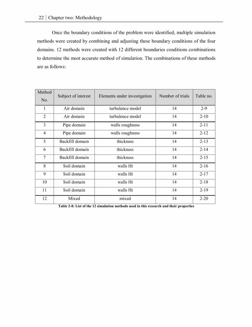
d. Soil domain boundary conditions (see figure 2-17 and table 2-7)
e. Linking all domains together
f. Write the solver file for simulator to process next step
21 Chapter two: Methodology
Full
name
Air
domain turbulence
Heat
transfer
Thermal
radiation
Inlet
temp.
Inlet
pressure
Inlet
velocity
Outlet
momentum
outlet
pressure
Code
name A- Tu Ht TR InT InP InV OM OP
Table 2-4: Air domain boundary conditions definitions
Full
name
Pipe
domain
Initial
temp.
Heat
transfer
Thermal
radiation
Code
name P- IT Ht TR
Table 2-5: Pipes domain boundary conditions definitions
Full
name
Backfill
domain
Initial
temp.
Heat
transfer
Thermal
radiation
Code
name B- IT Ht TR
Table 2-6: Backfill domain boundary conditions definitions
Full
name
Soil
domain
Initial
temp.
Heat
transfer
Thermal
radiation
face A
heat
transfer
face B
heat
transfer
face C
heat
transfer
face D
heat
transfer
face E
heat
transfer
Code
name S- IT Ht TR fA fB fC fD fE
Table 2-7: Soil domain boundary conditions definitions
Figure 2-17: Soil domain faces locations
22 Chapter two: Methodology
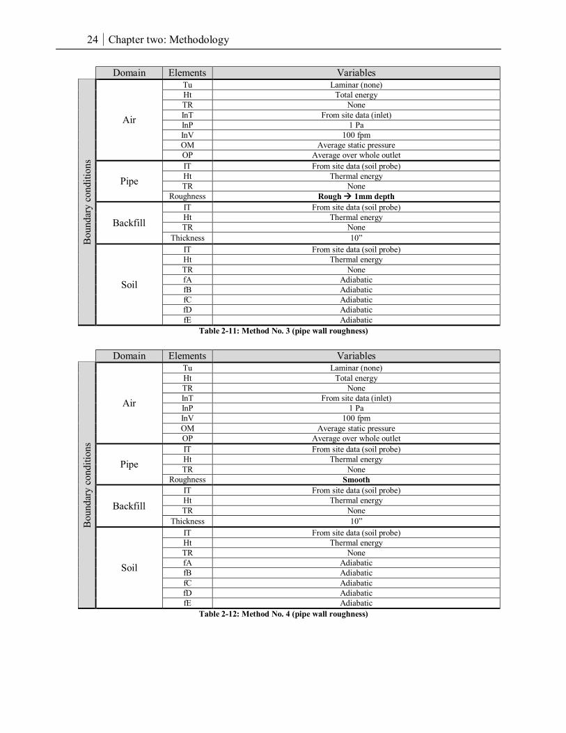
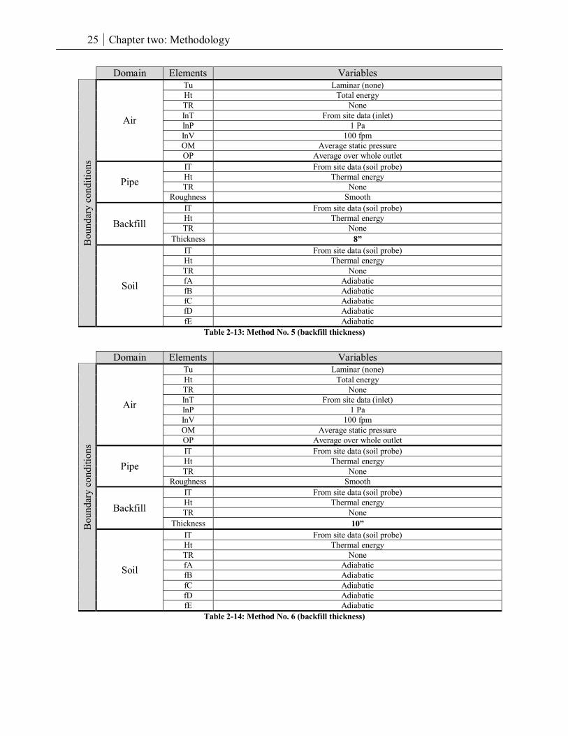
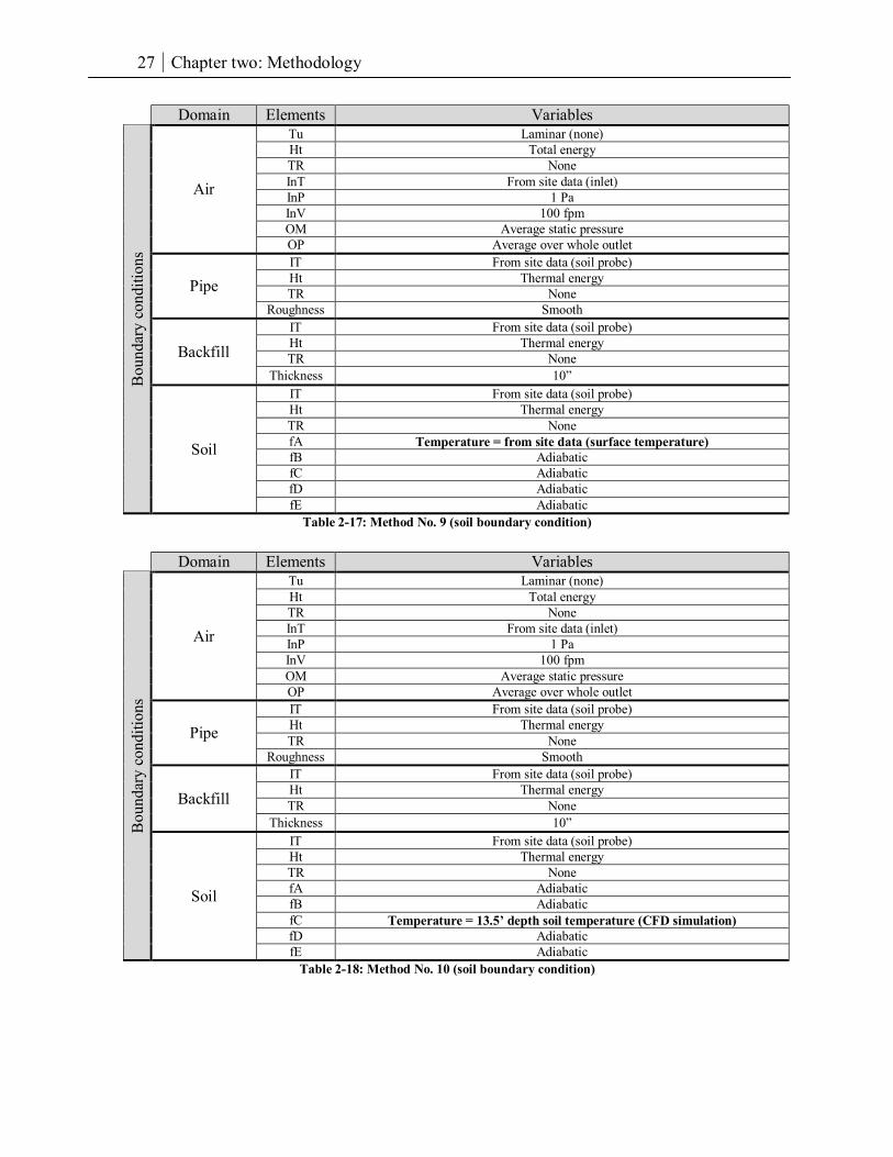
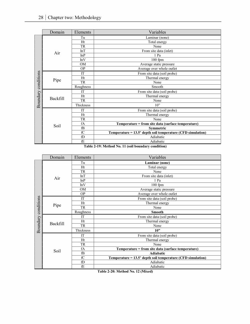
Once the boundary conditions of the problem were identified, multiple simulation
methods were created by combining and adjusting these boundary conditions of the four
domains. 12 methods were created with 12 different boundaries conditions combinations
to determine the most accurate method of simulation. The combinations of these methods
are as follows:
Method
No. Subject of interest Elements under investigation Number of trials Table no.
1 Air domain turbulence model 14 2-9
2 Air domain turbulence model 14 2-10
3 Pipe domain walls roughness 14 2-11
4 Pipe domain walls roughness 14 2-12
5 Backfill domain thickness 14 2-13
6 Backfill domain thickness 14 2-14
7 Backfill domain thickness 14 2-15
8 Soil domain walls Ht 14 2-16
9 Soil domain walls Ht 14 2-17
10 Soil domain walls Ht 14 2-18
11 Soil domain walls Ht 14 2-19
12 Mixed mixed 14 2-20 Table 2-8: List of the 12 simulation methods used in this research and their properties
23 Chapter two: Methodology
Domain Elements Variables B
ound
ary
cond
ition
s
Air
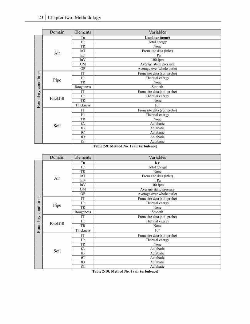
Tu Laminar (none) Ht Total energy TR None InT From site data (inlet) InP 1 Pa InV 100 fpm OM Average static pressure OP Average over whole outlet
Pipe IT From site data (soil probe) Ht Thermal energy TR None
Roughness Smooth
Backfill IT From site data (soil probe) Ht Thermal energy TR None
Thickness 10”
Soil
IT From site data (soil probe) Ht Thermal energy TR None fA Adiabatic fB Adiabatic fC Adiabatic fD Adiabatic fE Adiabatic
Table 2-9: Method No. 1 (air turbulence)
Domain Elements Variables
Bou
ndar
y co
nditi
ons
Air
Tu k-є Ht Total energy TR None InT From site data (inlet) InP 1 Pa InV 100 fpm OM Average static pressure OP Average over whole outlet
Pipe IT From site data (soil probe) Ht Thermal energy TR None
Roughness Smooth
Backfill IT From site data (soil probe) Ht Thermal energy TR None
Thickness 10”
Soil
IT From site data (soil probe) Ht Thermal energy TR None fA Adiabatic fB Adiabatic fC Adiabatic fD Adiabatic fE Adiabatic
Table 2-10: Method No. 2 (air turbulence)
24 Chapter two: Methodology
Domain Elements Variables B
ound
ary
cond
ition
s
Air
Tu Laminar (none) Ht Total energy TR None InT From site data (inlet) InP 1 Pa InV 100 fpm OM Average static pressure OP Average over whole outlet
Pipe IT From site data (soil probe) Ht Thermal energy TR None
Roughness Rough à 1mm depth
Backfill IT From site data (soil probe) Ht Thermal energy TR None
Thickness 10”
Soil
IT From site data (soil probe) Ht Thermal energy TR None fA Adiabatic fB Adiabatic fC Adiabatic fD Adiabatic fE Adiabatic
Table 2-11: Method No. 3 (pipe wall roughness)
Domain Elements Variables
Bou
ndar
y co
nditi
ons
Air
Tu Laminar (none) Ht Total energy TR None InT From site data (inlet) InP 1 Pa InV 100 fpm OM Average static pressure OP Average over whole outlet
Pipe IT From site data (soil probe) Ht Thermal energy TR None
Roughness Smooth
Backfill IT From site data (soil probe) Ht Thermal energy TR None
Thickness 10”
Soil
IT From site data (soil probe) Ht Thermal energy TR None fA Adiabatic fB Adiabatic fC Adiabatic fD Adiabatic fE Adiabatic
Table 2-12: Method No. 4 (pipe wall roughness)
25 Chapter two: Methodology
Domain Elements Variables B
ound
ary
cond
ition
s
Air
Tu Laminar (none) Ht Total energy TR None InT From site data (inlet) InP 1 Pa InV 100 fpm OM Average static pressure OP Average over whole outlet
Pipe IT From site data (soil probe) Ht Thermal energy TR None
Roughness Smooth
Backfill IT From site data (soil probe) Ht Thermal energy TR None
Thickness 8”
Soil
IT From site data (soil probe) Ht Thermal energy TR None fA Adiabatic fB Adiabatic fC Adiabatic fD Adiabatic fE Adiabatic
Table 2-13: Method No. 5 (backfill thickness)
Domain Elements Variables
Bou
ndar
y co
nditi
ons
Air
Tu Laminar (none) Ht Total energy TR None InT From site data (inlet) InP 1 Pa InV 100 fpm OM Average static pressure OP Average over whole outlet
Pipe IT From site data (soil probe) Ht Thermal energy TR None
Roughness Smooth
Backfill IT From site data (soil probe) Ht Thermal energy TR None
Thickness 10”
Soil
IT From site data (soil probe) Ht Thermal energy TR None fA Adiabatic fB Adiabatic fC Adiabatic fD Adiabatic fE Adiabatic
Table 2-14: Method No. 6 (backfill thickness)

26 Chapter two: Methodology
Domain Elements Variables B
ound
ary
cond
ition
s
Air
Tu Laminar (none) Ht Total energy TR None InT From site data (inlet) InP 1 Pa InV 100 fpm OM Average static pressure OP Average over whole outlet
Pipe IT From site data (soil probe) Ht Thermal energy TR None
Roughness Smooth
Backfill IT From site data (soil probe) Ht Thermal energy TR None
Thickness 12”
Soil
IT From site data (soil probe) Ht Thermal energy TR None fA Adiabatic fB Adiabatic fC Adiabatic fD Adiabatic fE Adiabatic
Table 2-15: Method No. 7 (backfill thickness)
Domain Elements Variables
Bou
ndar
y co
nditi
ons
Air
Tu Laminar (none) Ht Total energy TR None InT From site data (inlet) InP 1 Pa InV 100 fpm OM Average static pressure OP Average over whole outlet
Pipe IT From site data (soil probe) Ht Thermal energy TR None
Roughness Smooth
Backfill IT From site data (soil probe) Ht Thermal energy TR None
Thickness 10”
Soil
IT From site data (soil probe) Ht Thermal energy TR None fA Adiabatic fB Symmetric fC Adiabatic fD Adiabatic fE Adiabatic
Table 2-16: Method No. 8 (soil boundary condition)
27 Chapter two: Methodology
Domain Elements Variables B
ound
ary
cond
ition
s
Air
Tu Laminar (none) Ht Total energy TR None InT From site data (inlet) InP 1 Pa InV 100 fpm OM Average static pressure OP Average over whole outlet
Pipe IT From site data (soil probe) Ht Thermal energy TR None
Roughness Smooth
Backfill IT From site data (soil probe) Ht Thermal energy TR None
Thickness 10”
Soil
IT From site data (soil probe) Ht Thermal energy TR None fA Temperature = from site data (surface temperature) fB Adiabatic fC Adiabatic fD Adiabatic fE Adiabatic
Table 2-17: Method No. 9 (soil boundary condition)
Domain Elements Variables
Bou
ndar
y co
nditi
ons
Air
Tu Laminar (none) Ht Total energy TR None InT From site data (inlet) InP 1 Pa InV 100 fpm OM Average static pressure OP Average over whole outlet
Pipe IT From site data (soil probe) Ht Thermal energy TR None
Roughness Smooth
Backfill IT From site data (soil probe) Ht Thermal energy TR None
Thickness 10”
Soil
IT From site data (soil probe) Ht Thermal energy TR None fA Adiabatic fB Adiabatic fC Temperature = 13.5’ depth soil temperature (CFD simulation) fD Adiabatic fE Adiabatic
Table 2-18: Method No. 10 (soil boundary condition)
28 Chapter two: Methodology
Domain Elements Variables B
ound
ary
cond
ition
s
Air
Tu Laminar (none) Ht Total energy TR None InT From site data (inlet) InP 1 Pa InV 100 fpm OM Average static pressure OP Average over whole outlet
Pipe IT From site data (soil probe) Ht Thermal energy TR None
Roughness Smooth
Backfill IT From site data (soil probe) Ht Thermal energy TR None
Thickness 10”
Soil
IT From site data (soil probe) Ht Thermal energy TR None fA Temperature = from site data (surface temperature) fB Symmetric fC Temperature = 13.5’ depth soil temperature (CFD simulation) fD Adiabatic fE Adiabatic
Table 2-19: Method No. 11 (soil boundary condition)
Domain Elements Variables
Bou
ndar
y co
nditi
ons
Air
Tu Laminar (none) Ht Total energy TR None InT From site data (inlet) InP 1 Pa InV 100 fpm OM Average static pressure OP Average over whole outlet
Pipe IT From site data (soil probe) Ht Thermal energy TR None
Roughness Smooth
Backfill IT From site data (soil probe) Ht Thermal energy TR None
Thickness 10”
Soil
IT From site data (soil probe) Ht Thermal energy TR None fA Temperature = from site data (surface temperature) fB Adiabatic fC Temperature = 13.5’ depth soil temperature (CFD simulation) fD Adiabatic fE Adiabatic
Table 2-20: Method No. 12 (Mixed)
29 Chapter two: Methodology
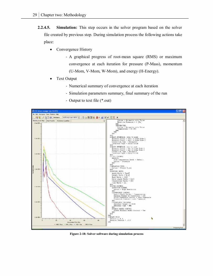
2.2.4.5. Simulation: This step occurs in the solver program based on the solver
file created by previous step. During simulation process the following actions take
place:
• Convergence History
- A graphical progress of root-mean square (RMS) or maximum
convergence at each iteration for pressure (P-Mass), momentum
(U-Mom, V-Mom, W-Mom), and energy (H-Energy).
• Text Output
- Numerical summary of convergence at each iteration
- Simulation parameters summary, final summary of the run
- Output to text file (*.out)
Figure 2-18: Solver software during simulation process
30 Chapter two: Methodology
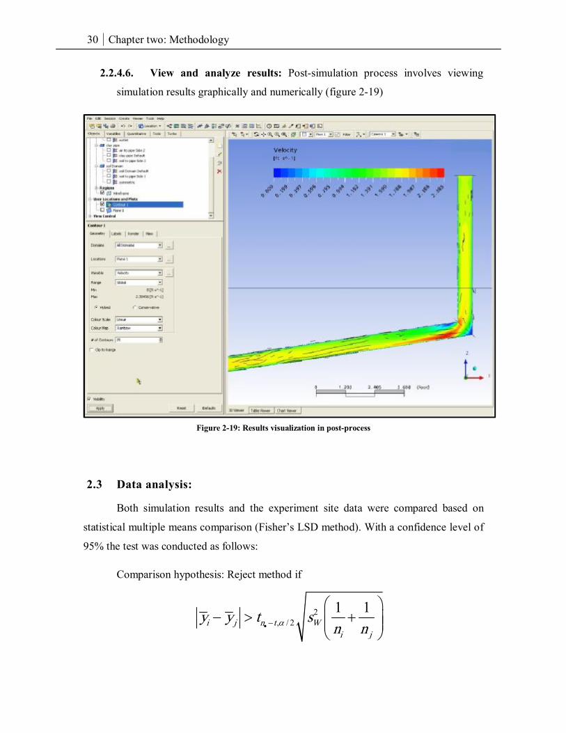
2.2.4.6. View and analyze results: Post-simulation process involves viewing
simulation results graphically and numerically (figure 2-19)
Figure 2-19: Results visualization in post-process
2.3 Data analysis:
Both simulation results and the experiment site data were compared based on
statistical multiple means comparison (Fisher’s LSD method). With a confidence level of
95% the test was conducted as follows:
Comparison hypothesis: Reject method if
2, / 2
1 1i j n t W
i j
y y t sn nα• −
− > +
31 Chapter three: Results
3. Chapter three: Results This chapter will summarize the outcome of this research under five categories:
1. Experimental site monitoring and comparisons results
2. CFD tools comparative investigation results
3. CFD software testing results
4. Soil sample simulation results
5. GCV system modeling methods simulation results
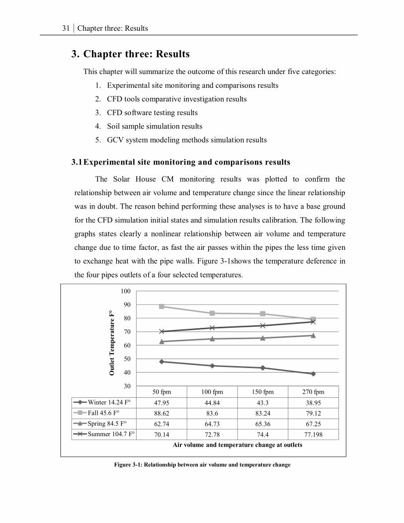
3.1 Experimental site monitoring and comparisons results
The Solar House CM monitoring results was plotted to confirm the
relationship between air volume and temperature change since the linear relationship
was in doubt. The reason behind performing these analyses is to have a base ground
for the CFD simulation initial states and simulation results calibration. The following
graphs states clearly a nonlinear relationship between air volume and temperature
change due to time factor, as fast the air passes within the pipes the less time given
to exchange heat with the pipe walls. Figure 3-1shows the temperature deference in
the four pipes outlets of a four selected temperatures.
Figure 3-1: Relationship between air volume and temperature change
50 fpm 100 fpm 150 fpm 270 fpmWinter 14.24 F° 47.95 44.84 43.3 38.95Fall 45.6 F° 88.62 83.6 83.24 79.12Spring 84.5 F° 62.74 64.73 65.36 67.25Summer 104.7 F° 70.14 72.78 74.4 77.198
30
40
50
60
70
80
90
100
Out
let T
empe
ratu
re F
°
Air volume and temperature change at outlets
32 Chapter three: Results
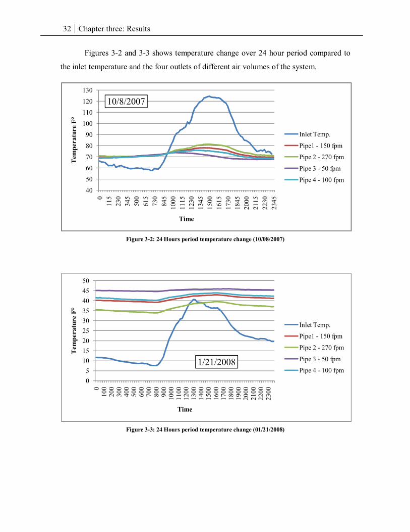
Figures 3-2 and 3-3 shows temperature change over 24 hour period compared to
the inlet temperature and the four outlets of different air volumes of the system.
Figure 3-2: 24 Hours period temperature change (10/08/2007)
Figure 3-3: 24 Hours period temperature change (01/21/2008)
40
50
60
70
80
90
100
110
120
1300
115
230
345
500
615
730
845
1000
1115
1230
1345
1500
1615
1730
1845
2000
2115
2230
2345
Tem
pera
ture
F°
Time
10/8/2007
Inlet Temp.
Pipe1 - 150 fpm
Pipe 2 - 270 fpm
Pipe 3 - 50 fpm
Pipe 4 - 100 fpm
05
101520253035404550
010
020
030
040
050
060
070
080
090
010
0011
0012
0013
0014
0015
0016
0017
0018
0019
0020
0021
0022
0023
00
Tem
pera
ture
F°
Time
1/21/2008
Inlet Temp.
Pipe1 - 150 fpm
Pipe 2 - 270 fpm
Pipe 3 - 50 fpm
Pipe 4 - 100 fpm
33 Chapter three: Results
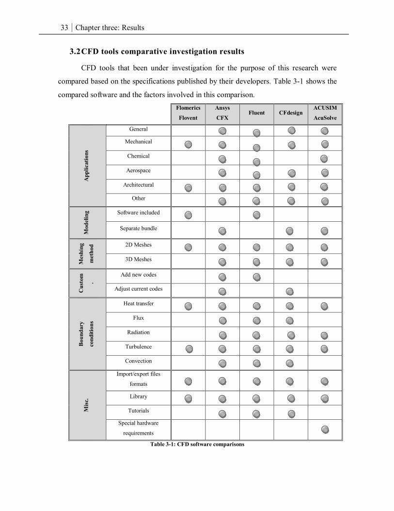
3.2 CFD tools comparative investigation results
CFD tools that been under investigation for the purpose of this research were
compared based on the specifications published by their developers. Table 3-1 shows the
compared software and the factors involved in this comparison.
Flomerics
Flovent
Ansys
CFX Fluent CFdesign
ACUSIM
AcuSolve
App
licat
ions
General
Mechanical
Chemical
Aerospace
Architectural
Other
Mod
elin
g Software included
Separate bundle
Mes
hing
met
hod 2D Meshes
3D Meshes
Cus
tom
.
Add new codes
Adjust current codes
Boun
dary
cond
ition
s
Heat transfer
Flux
Radiation
Turbulence
Convection
Misc
.
Import/export files
formats
Library
Tutorials
Special hardware
requirements
Table 3-1: CFD software comparisons
34 Chapter three: Results
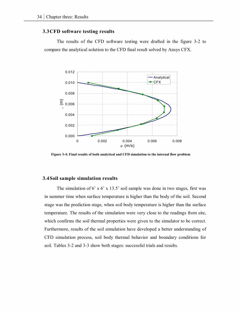
3.3 CFD software testing results
The results of the CFD software testing were drafted in the figure 3-2 to
compare the analytical solution to the CFD final result solved by Ansys CFX.
Figure 3-4: Final results of both analytical and CFD simulation to the internal flow problem
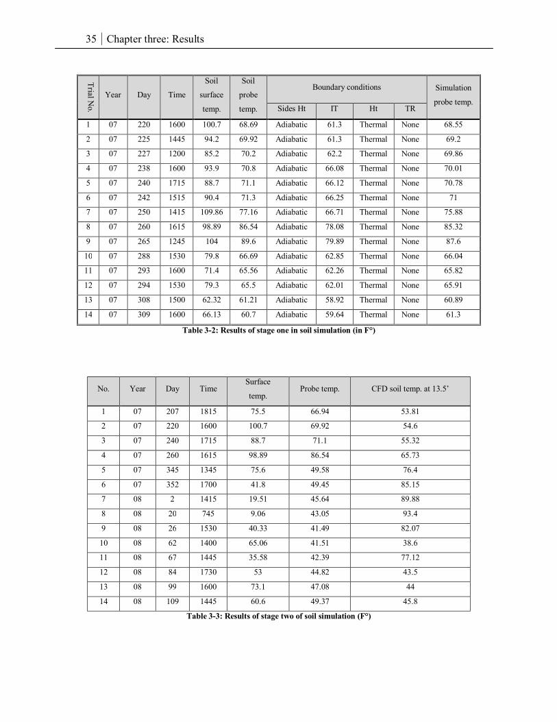
3.4 Soil sample simulation results
The simulation of 6’ x 6’ x 13.5’ soil sample was done in two stages, first was
in summer time when surface temperature is higher than the body of the soil. Second
stage was the prediction stage, when soil body temperature is higher than the surface
temperature. The results of the simulation were very close to the readings from site,
which confirms the soil thermal properties were given to the simulator to be correct.
Furthermore, results of the soil simulation have developed a better understanding of
CFD simulation process, soil body thermal behavior and boundary conditions for
soil. Tables 3-2 and 3-3 show both stages: successful trials and results.
0.000
0.002
0.004
0.006
0.008
0.010
0.012
0 0.002 0.004 0.006 0.008u (m/s)
y
(m)
AnalyticalCFX
35 Chapter three: Results
Table 3-2: Results of stage one in soil simulation (in F°)
No. Year Day Time Surface
temp. Probe temp. CFD soil temp. at 13.5’
1 07 207 1815 75.5 66.94 53.81
2 07 220 1600 100.7 69.92 54.6
3 07 240 1715 88.7 71.1 55.32
4 07 260 1615 98.89 86.54 65.73
5 07 345 1345 75.6 49.58 76.4
6 07 352 1700 41.8 49.45 85.15
7 08 2 1415 19.51 45.64 89.88
8 08 20 745 9.06 43.05 93.4
9 08 26 1530 40.33 41.49 82.07
10 08 62 1400 65.06 41.51 38.6
11 08 67 1445 35.58 42.39 77.12
12 08 84 1730 53 44.82 43.5
13 08 99 1600 73.1 47.08 44
14 08 109 1445 60.6 49.37 45.8
Table 3-3: Results of stage two of soil simulation (F°)
Trial No.
Year Day Time
Soil
surface
temp.
Soil
probe
temp.
Boundary conditions Simulation
probe temp. Sides Ht IT Ht TR
1 07 220 1600 100.7 68.69 Adiabatic 61.3 Thermal None 68.55
2 07 225 1445 94.2 69.92 Adiabatic 61.3 Thermal None 69.2
3 07 227 1200 85.2 70.2 Adiabatic 62.2 Thermal None 69.86
4 07 238 1600 93.9 70.8 Adiabatic 66.08 Thermal None 70.01
5 07 240 1715 88.7 71.1 Adiabatic 66.12 Thermal None 70.78
6 07 242 1515 90.4 71.3 Adiabatic 66.25 Thermal None 71
7 07 250 1415 109.86 77.16 Adiabatic 66.71 Thermal None 75.88
8 07 260 1615 98.89 86.54 Adiabatic 78.08 Thermal None 85.32
9 07 265 1245 104 89.6 Adiabatic 79.89 Thermal None 87.6
10 07 288 1530 79.8 66.69 Adiabatic 62.85 Thermal None 66.04
11 07 293 1600 71.4 65.56 Adiabatic 62.26 Thermal None 65.82
12 07 294 1530 79.3 65.5 Adiabatic 62.01 Thermal None 65.91
13 07 308 1500 62.32 61.21 Adiabatic 58.92 Thermal None 60.89
14 07 309 1600 66.13 60.7 Adiabatic 59.64 Thermal None 61.3
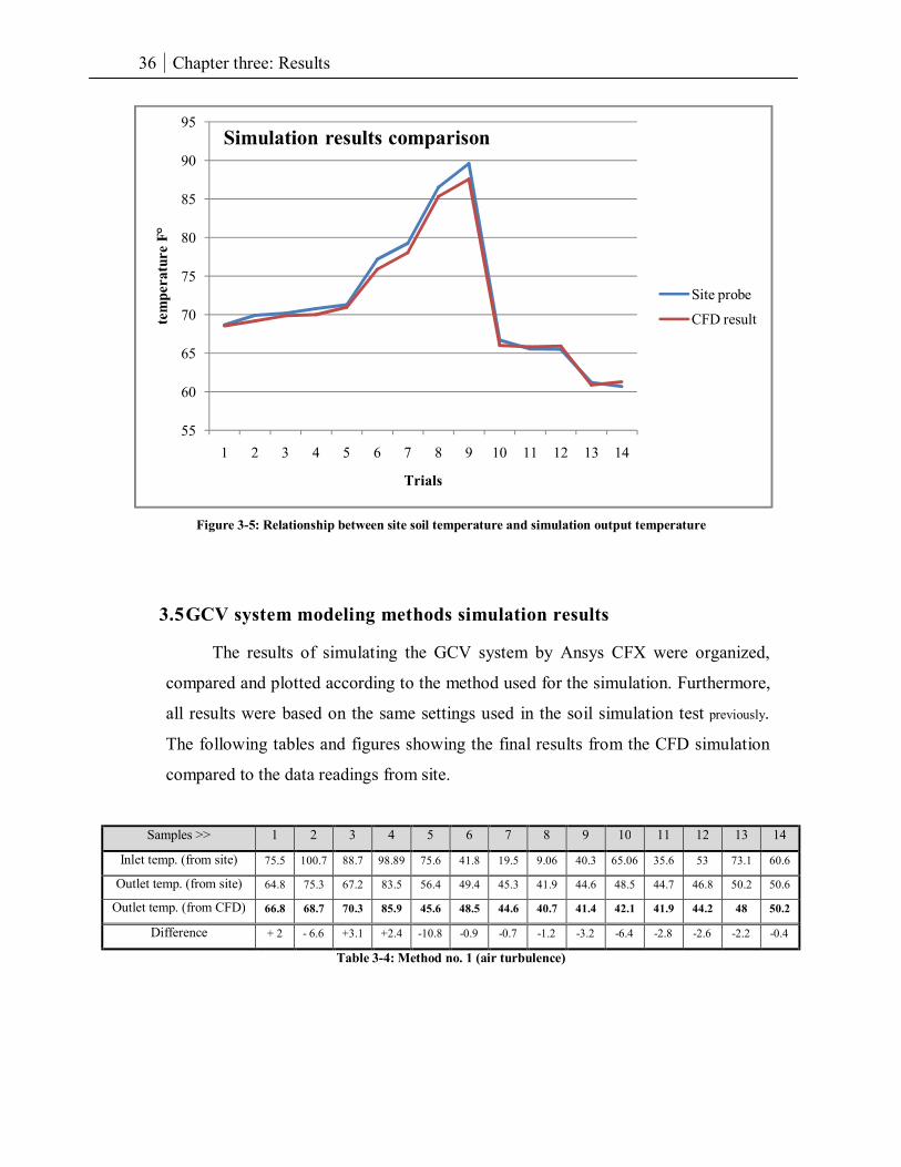
36 Chapter three: Results
Figure 3-5: Relationship between site soil temperature and simulation output temperature
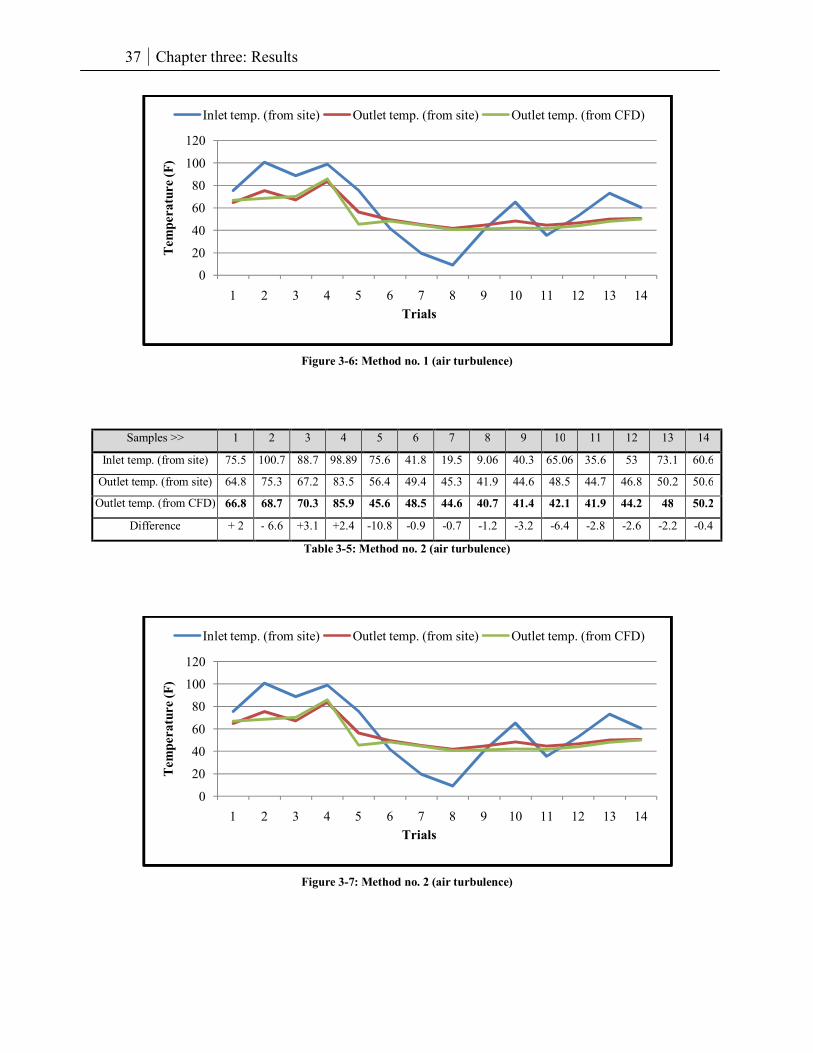
3.5 GCV system modeling methods simulation results
The results of simulating the GCV system by Ansys CFX were organized,
compared and plotted according to the method used for the simulation. Furthermore,
all results were based on the same settings used in the soil simulation test previously.
The following tables and figures showing the final results from the CFD simulation
compared to the data readings from site.
Samples >> 1 2 3 4 5 6 7 8 9 10 11 12 13 14
Inlet temp. (from site) 75.5 100.7 88.7 98.89 75.6 41.8 19.5 9.06 40.3 65.06 35.6 53 73.1 60.6
Outlet temp. (from site) 64.8 75.3 67.2 83.5 56.4 49.4 45.3 41.9 44.6 48.5 44.7 46.8 50.2 50.6
Outlet temp. (from CFD) 66.8 68.7 70.3 85.9 45.6 48.5 44.6 40.7 41.4 42.1 41.9 44.2 48 50.2
Difference + 2 - 6.6 +3.1 +2.4 -10.8 -0.9 -0.7 -1.2 -3.2 -6.4 -2.8 -2.6 -2.2 -0.4
Table 3-4: Method no. 1 (air turbulence)
55
60
65
70
75
80
85
90
95
1 2 3 4 5 6 7 8 9 10 11 12 13 14
tem
pera
ture
F°
Trials
Simulation results comparison
Site probe
CFD result
37 Chapter three: Results
Figure 3-6: Method no. 1 (air turbulence)
Samples >> 1 2 3 4 5 6 7 8 9 10 11 12 13 14
Inlet temp. (from site) 75.5 100.7 88.7 98.89 75.6 41.8 19.5 9.06 40.3 65.06 35.6 53 73.1 60.6
Outlet temp. (from site) 64.8 75.3 67.2 83.5 56.4 49.4 45.3 41.9 44.6 48.5 44.7 46.8 50.2 50.6
Outlet temp. (from CFD) 66.8 68.7 70.3 85.9 45.6 48.5 44.6 40.7 41.4 42.1 41.9 44.2 48 50.2
Difference + 2 - 6.6 +3.1 +2.4 -10.8 -0.9 -0.7 -1.2 -3.2 -6.4 -2.8 -2.6 -2.2 -0.4
Table 3-5: Method no. 2 (air turbulence)
Figure 3-7: Method no. 2 (air turbulence)
0
20
40
60
80
100
120
1 2 3 4 5 6 7 8 9 10 11 12 13 14
Tem
pera
ture
(F)
Trials
Inlet temp. (from site) Outlet temp. (from site) Outlet temp. (from CFD)
0
20
40
60
80
100
120
1 2 3 4 5 6 7 8 9 10 11 12 13 14
Tem
pera
ture
(F)
Trials
Inlet temp. (from site) Outlet temp. (from site) Outlet temp. (from CFD)
38 Chapter three: Results
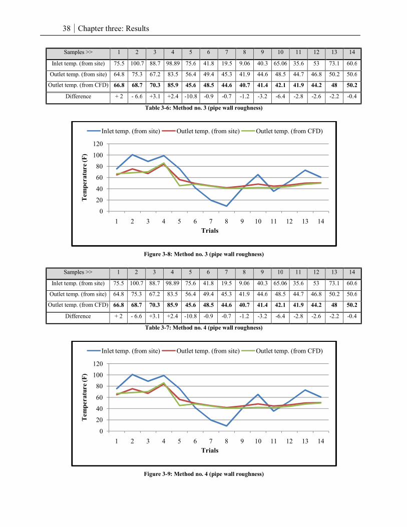
Samples >> 1 2 3 4 5 6 7 8 9 10 11 12 13 14
Inlet temp. (from site) 75.5 100.7 88.7 98.89 75.6 41.8 19.5 9.06 40.3 65.06 35.6 53 73.1 60.6
Outlet temp. (from site) 64.8 75.3 67.2 83.5 56.4 49.4 45.3 41.9 44.6 48.5 44.7 46.8 50.2 50.6
Outlet temp. (from CFD) 66.8 68.7 70.3 85.9 45.6 48.5 44.6 40.7 41.4 42.1 41.9 44.2 48 50.2
Difference + 2 - 6.6 +3.1 +2.4 -10.8 -0.9 -0.7 -1.2 -3.2 -6.4 -2.8 -2.6 -2.2 -0.4
Table 3-6: Method no. 3 (pipe wall roughness)
Figure 3-8: Method no. 3 (pipe wall roughness)
Samples >> 1 2 3 4 5 6 7 8 9 10 11 12 13 14
Inlet temp. (from site) 75.5 100.7 88.7 98.89 75.6 41.8 19.5 9.06 40.3 65.06 35.6 53 73.1 60.6
Outlet temp. (from site) 64.8 75.3 67.2 83.5 56.4 49.4 45.3 41.9 44.6 48.5 44.7 46.8 50.2 50.6
Outlet temp. (from CFD) 66.8 68.7 70.3 85.9 45.6 48.5 44.6 40.7 41.4 42.1 41.9 44.2 48 50.2
Difference + 2 - 6.6 +3.1 +2.4 -10.8 -0.9 -0.7 -1.2 -3.2 -6.4 -2.8 -2.6 -2.2 -0.4
Table 3-7: Method no. 4 (pipe wall roughness)
Figure 3-9: Method no. 4 (pipe wall roughness)
0
20
40
60
80
100
120
1 2 3 4 5 6 7 8 9 10 11 12 13 14
Tem
pera
ture
(F)
Trials
Inlet temp. (from site) Outlet temp. (from site) Outlet temp. (from CFD)
0
20
40
60
80
100
120
1 2 3 4 5 6 7 8 9 10 11 12 13 14
Tem
pera
ture
(F)
Trials
Inlet temp. (from site) Outlet temp. (from site) Outlet temp. (from CFD)
39 Chapter three: Results
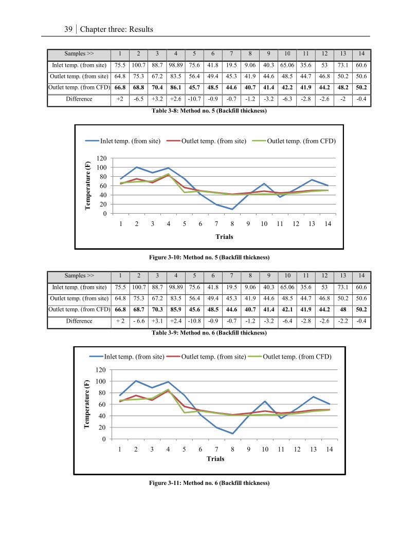
Samples >> 1 2 3 4 5 6 7 8 9 10 11 12 13 14
Inlet temp. (from site) 75.5 100.7 88.7 98.89 75.6 41.8 19.5 9.06 40.3 65.06 35.6 53 73.1 60.6
Outlet temp. (from site) 64.8 75.3 67.2 83.5 56.4 49.4 45.3 41.9 44.6 48.5 44.7 46.8 50.2 50.6
Outlet temp. (from CFD) 66.8 68.8 70.4 86.1 45.7 48.5 44.6 40.7 41.4 42.2 41.9 44.2 48.2 50.2
Difference +2 -6.5 +3.2 +2.6 -10.7 -0.9 -0.7 -1.2 -3.2 -6.3 -2.8 -2.6 -2 -0.4
Table 3-8: Method no. 5 (Backfill thickness)
Figure 3-10: Method no. 5 (Backfill thickness)
Samples >> 1 2 3 4 5 6 7 8 9 10 11 12 13 14
Inlet temp. (from site) 75.5 100.7 88.7 98.89 75.6 41.8 19.5 9.06 40.3 65.06 35.6 53 73.1 60.6
Outlet temp. (from site) 64.8 75.3 67.2 83.5 56.4 49.4 45.3 41.9 44.6 48.5 44.7 46.8 50.2 50.6
Outlet temp. (from CFD) 66.8 68.7 70.3 85.9 45.6 48.5 44.6 40.7 41.4 42.1 41.9 44.2 48 50.2
Difference + 2 - 6.6 +3.1 +2.4 -10.8 -0.9 -0.7 -1.2 -3.2 -6.4 -2.8 -2.6 -2.2 -0.4
Table 3-9: Method no. 6 (Backfill thickness)
Figure 3-11: Method no. 6 (Backfill thickness)
020406080
100120
1 2 3 4 5 6 7 8 9 10 11 12 13 14
Tem
pera
ture
(F)
Trials
Inlet temp. (from site) Outlet temp. (from site) Outlet temp. (from CFD)
0
20
40
60
80
100
120
1 2 3 4 5 6 7 8 9 10 11 12 13 14
Tem
pera
ture
(F)
Trials
Inlet temp. (from site) Outlet temp. (from site) Outlet temp. (from CFD)
40 Chapter three: Results
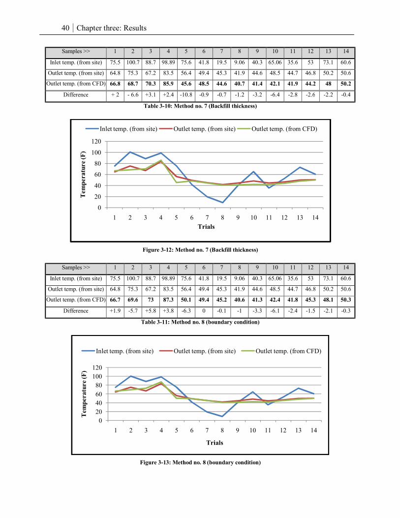
Samples >> 1 2 3 4 5 6 7 8 9 10 11 12 13 14
Inlet temp. (from site) 75.5 100.7 88.7 98.89 75.6 41.8 19.5 9.06 40.3 65.06 35.6 53 73.1 60.6
Outlet temp. (from site) 64.8 75.3 67.2 83.5 56.4 49.4 45.3 41.9 44.6 48.5 44.7 46.8 50.2 50.6
Outlet temp. (from CFD) 66.8 68.7 70.3 85.9 45.6 48.5 44.6 40.7 41.4 42.1 41.9 44.2 48 50.2
Difference + 2 - 6.6 +3.1 +2.4 -10.8 -0.9 -0.7 -1.2 -3.2 -6.4 -2.8 -2.6 -2.2 -0.4
Table 3-10: Method no. 7 (Backfill thickness)
Figure 3-12: Method no. 7 (Backfill thickness)
Samples >> 1 2 3 4 5 6 7 8 9 10 11 12 13 14
Inlet temp. (from site) 75.5 100.7 88.7 98.89 75.6 41.8 19.5 9.06 40.3 65.06 35.6 53 73.1 60.6
Outlet temp. (from site) 64.8 75.3 67.2 83.5 56.4 49.4 45.3 41.9 44.6 48.5 44.7 46.8 50.2 50.6
Outlet temp. (from CFD) 66.7 69.6 73 87.3 50.1 49.4 45.2 40.6 41.3 42.4 41.8 45.3 48.1 50.3
Difference +1.9 -5.7 +5.8 +3.8 -6.3 0 -0.1 -1 -3.3 -6.1 -2.4 -1.5 -2.1 -0.3
Table 3-11: Method no. 8 (boundary condition)
Figure 3-13: Method no. 8 (boundary condition)
0
20
40
60
80
100
120
1 2 3 4 5 6 7 8 9 10 11 12 13 14
Tem
pera
ture
(F)
Trials
Inlet temp. (from site) Outlet temp. (from site) Outlet temp. (from CFD)
020406080
100120
1 2 3 4 5 6 7 8 9 10 11 12 13 14
Tem
pera
ture
(F)
Trials
Inlet temp. (from site) Outlet temp. (from site) Outlet temp. (from CFD)
41 Chapter three: Results
Samples >> 1 2 3 4 5 6 7 8 9 10 11 12 13 14
Inlet temp. (from site) 75.5 100.7 88.7 98.89 75.6 41.8 19.5 9.06 40.3 65.06 35.6 53 73.1 60.6
Outlet temp. (from site) 64.8 75.3 67.2 83.5 56.4 49.4 45.3 41.9 44.6 48.5 44.7 46.8 50.2 50.6
Outlet temp. (from CFD) 70.7 79.4 78 90.8 56.6 43.5 40.1 31.2 41.1 48.1 41.6 47.2 56.3 52.1
Difference +5.9 +4.1 +10.8 +7.3 +0.2 -5.9 -5.2 -10.7 -3.5 -0.4 -3.1 +0.4 +6.1 +1.5
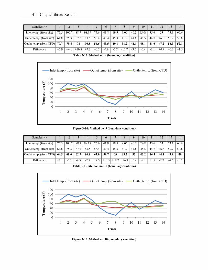
Table 3-12: Method no. 9 (boundary condition)
Figure 3-14: Method no. 9 (boundary condition)
Samples >> 1 2 3 4 5 6 7 8 9 10 11 12 13 14
Inlet temp. (from site) 75.5 100.7 88.7 98.89 75.6 41.8 19.5 9.06 40.3 65.06 35.6 53 73.1 60.6
Outlet temp. (from site) 64.8 75.3 67.2 83.5 56.4 49.4 45.3 41.9 44.6 48.5 44.7 46.8 50.2 50.6
Outlet temp. (from CFD) 64.5 68.6 62.7 80.8 63.9 59.7 69 68.3 50 40.2 46.5 44.1 45.9 49
Difference -0.3 -6.7 -4.5 -2.7 +7.5 +10.3 +18.7 +26.4 +5.4 -8.3 +1.8 -2.7 -4.3 -1.6
Table 3-13: Method no. 10 (boundary condition)
Figure 3-15: Method no. 10 (boundary condition)
020406080
100120
1 2 3 4 5 6 7 8 9 10 11 12 13 14
Tem
pera
ture
(F)
Trials
Inlet temp. (from site) Outlet temp. (from site) Outlet temp. (from CFD)
020406080
100120
1 2 3 4 5 6 7 8 9 10 11 12 13 14
Tem
pera
ture
(F)
Trials
Inlet temp. (from site) Outlet temp. (from site) Outlet temp. (from CFD)
42 Chapter three: Results
Samples >> 1 2 3 4 5 6 7 8 9 10 11 12 13 14
Inlet temp. (from site) 75.5 100.7 88.7 98.89 75.6 41.8 19.5 9.06 40.3 65.06 35.6 53 73.1 60.6
Outlet temp. (from site) 64.8 75.3 67.2 83.5 56.4 49.4 45.3 41.9 44.6 48.5 44.7 46.8 50.2 50.6
Outlet temp. (from CFD) 66.7 69.6 73 87.3 50.1 49.4 45.2 40.6 41.3 42.4 41.8 45.3 48.1 50.3
Difference +1.9 -5.7 +5.8 +3.8 -6.3 0 -0.1 -1 -3.3 -6.1 -2.4 -1.5 -2.1 -0.3
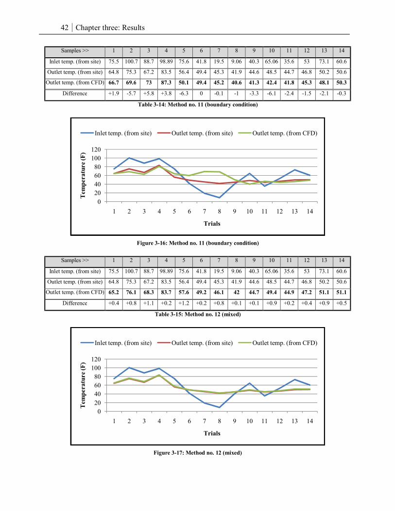
Table 3-14: Method no. 11 (boundary condition)
Figure 3-16: Method no. 11 (boundary condition)
Samples >> 1 2 3 4 5 6 7 8 9 10 11 12 13 14
Inlet temp. (from site) 75.5 100.7 88.7 98.89 75.6 41.8 19.5 9.06 40.3 65.06 35.6 53 73.1 60.6
Outlet temp. (from site) 64.8 75.3 67.2 83.5 56.4 49.4 45.3 41.9 44.6 48.5 44.7 46.8 50.2 50.6
Outlet temp. (from CFD) 65.2 76.1 68.3 83.7 57.6 49.2 46.1 42 44.7 49.4 44.9 47.2 51.1 51.1
Difference +0.4 +0.8 +1.1 +0.2 +1.2 +0.2 +0.8 +0.1 +0.1 +0.9 +0.2 +0.4 +0.9 +0.5
Table 3-15: Method no. 12 (mixed)
Figure 3-17: Method no. 12 (mixed)
020406080
100120
1 2 3 4 5 6 7 8 9 10 11 12 13 14
Tem
pera
ture
(F)
Trials
Inlet temp. (from site) Outlet temp. (from site) Outlet temp. (from CFD)
020406080
100120
1 2 3 4 5 6 7 8 9 10 11 12 13 14
Tem
pera
ture
(F)
Trials
Inlet temp. (from site) Outlet temp. (from site) Outlet temp. (from CFD)
43 Chapter three: Results
3.6 Data analysis results
In order to determine the best approach in simulation using one of the
previous methods a statistical test was made. Based on Fisher’s LSD means
comparison method the following table shows the results were concluded:
Method Mean Hypothesis test result
(|yi- 55.993| > 1.805)
1 52.778 Rejected
2 52.778 Rejected
3 52.778 Rejected
4 52.778 Rejected
5 52.835 Rejected
6 52.778 Rejected
7 52.778 Rejected
8 53.65 Rejected
9 55.478 Rejected
10 58.085 Rejected
11 58.085 Rejected
12 55.471 Accepted
Table 3-16: Simulation data statistical comparison results via Fisher’s LSD means comparison method
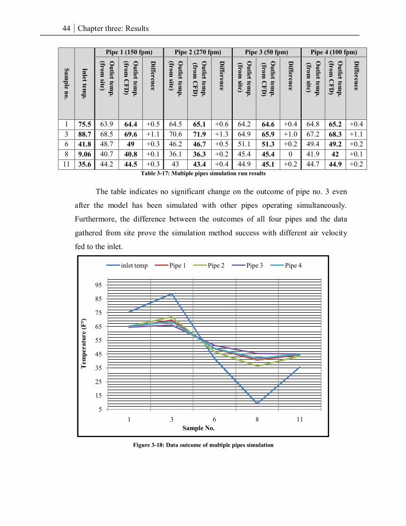
3.7 Multiple pipes simulation:
The purpose of this simulation is to find out if there a significant effect on
GCV performance when operating multiple pipes at the same time and the same
area. So far, the CFD simulation shows no effect on the performance and/or outcome
of these GCV systems on the steady state runs. Table 3-17 shows a comparison
between all four pipes simulation results based on the 12th method approach.
44 Chapter three: Results
Sample no.
Inlet temp.
Pipe 1 (150 fpm) Pipe 2 (270 fpm) Pipe 3 (50 fpm) Pipe 4 (100 fpm)
Outlet tem
p. (from
site)
Outlet tem
p. (from
CFD
)
Difference
Outlet tem
p. (from
site)
Outlet tem
p. (from
CFD
)
Difference
Outlet tem
p. (from
site)
Outlet tem
p. (from
CFD
)
Difference
Outlet tem
p. (from
site)
Outlet tem
p. (from
CFD
)
Difference
1 75.5 63.9 64.4 +0.5 64.5 65.1 +0.6 64.2 64.6 +0.4 64.8 65.2 +0.4 3 88.7 68.5 69.6 +1.1 70.6 71.9 +1.3 64.9 65.9 +1.0 67.2 68.3 +1.1 6 41.8 48.7 49 +0.3 46.2 46.7 +0.5 51.1 51.3 +0.2 49.4 49.2 +0.2 8 9.06 40.7 40.8 +0.1 36.1 36.3 +0.2 45.4 45.4 0 41.9 42 +0.1
11 35.6 44.2 44.5 +0.3 43 43.4 +0.4 44.9 45.1 +0.2 44.7 44.9 +0.2 Table 3-17: Multiple pipes simulation run results
The table indicates no significant change on the outcome of pipe no. 3 even
after the model has been simulated with other pipes operating simultaneously.
Furthermore, the difference between the outcomes of all four pipes and the data
gathered from site prove the simulation method success with different air velocity
fed to the inlet.
Figure 3-18: Data outcome of multiple pipes simulation
5
15
25
35
45
55
65
75
85
95
1 3 6 8 11
Tem
pera
ture
(F°)
Sample No.
inlet temp Pipe 1 Pipe 2 Pipe 3 Pipe 4
45 Chapter Four: Conclusions
4. Chapter Four: Conclusions This research was conducted to develop the best approach of simulation for
GCV systems through CFD tools. All contributing factors to the GCV system
performance were taken under consideration in the modeling and solving phases.
The main model of CFD simulation was digital imitation to the GCV system of
Virginia Tech Solar House CM (1981) Blacksburg, VA. From the results of each
step performed in this research, the following can be concluded:
• Solar house monitoring: results confirm that the relationship between
heat transfer and air velocity is a non-linear relationship. Furthermore, the
slower air passes through the system pipes the higher temperature change
occur.
• CFD tools investigation: for available CFD tools in the market, basic and
through comparison suggest using Ansys CFX as primary candidate for
this research purposes. This software has all needed components to
perform all required elements in this research.
• Soil sample simulation: first phase of soil simulation run proved the
accuracy of soil thermal properties claimed by the U.S Department Of
Energy. Next phase was made to predict the soil body temperature based
on data from the Solar House. These predictions are essential for the main
GCV simulation later.
• Single pipe simulation: the results of simulating 14 samples by twelve
different methods provide a clear evidence of the delicacy of soil domain
temperature initial setting and how it affects the results. The 12th method
was proved to be the best approach to simulate the GCV system and that is
the main objective of this research. This method includes non-turbulent air
flow at 100 fpm, smooth pipe surface, a 4” backfill thickness, soil surface
temperature taken from site and finally, soil temperature at 13.5’ taken
from soil sample simulation.
• Multiple pipes simulation: the effect of simulating multiple pipes per
model in a steady-state method shows no effect on the outcome of each
pipe simulated in this model.
46 <Works Cited
Works Cited 1. Ansys. (2007, December 12). cfx models radiation. Retrieved March 14, 2008, from
ANSYS, Inc. web site: http://www.ansys.com/products/cfx/cfx-models-radiation.asp
2. ASHRAE. (1999). Ventilation for Acceptable Indoor Air Quality. ANSI/ASHRAE
Standard 62.
3. Bernier, M. A. (2006). Closed-Loop Ground-Coupled Heat Pump Systems. ASHRAE Journal , 8.
4. Bruderer, H. (2005). Cooling with Heat Pumps: Passive and Active. Allendorf:
Viessmann (Schweiz) AG, Division SATAG Thermotechnics.
5. CFD-Online. (2008, Feberuary 9). Main Page. Retrieved March 13, 2008, from CFD
Online: http://www.cfd-online.com/Wiki/Main_Page
6. Couvillion, R. J., & Cotton, D. E. (1990). Laboratory and Computer Comparisons of Ground-Coupled Heat Pump Backfills. Atlanta ,GA: ASHRAE Trans.
7. Deru, M., Judkoff, R., & Neymark, J. (2003). Whole-Building Energy Simulation with a Three-Dimensional Ground-Coupled Heat Transfer Model. Atlanta ,GA: ASHRAE
Transactions.
8. Energy, D. o. (2008, Feberuary 1). EERE Consumer's Guide: Geothermal Heat Pumps. Retrieved May 5, 2008, from Department of Energy - Homepage:
http://www.eere.energy.gov/consumer/your_home/space_heating_cooling/index.cfm/
mytopic=12640
9. Fluent. (2007, August 28). A Brief History of Computational Fluid Dynamics (CFD)
from Fluent. Retrieved May 21, 2008, from Fluent:
http://www.fluent.com/about/cfdhistory.htm
10. Fluent. (n.d.). Fluent. Retrieved January 6, 2008, from A Brief History of
Computational Fluid Dynamics (CFD): http://www.fluent.com/about/cfdhistory.htm
11. Hillel, D. (1982). Introduction to soil physics. San Diego, CA: Academic Press.
47 <Works Cited
12. HPC. (2007, November 2). Heat Pump Centre. Retrieved December 21, 2007, from
Heat Pump Centre: http://www.heatpumpcentre.org/
13. Hyde, R. (2000). Climate Responsive Design. London and New York: E & FN Spon.
14. IEA. (2007, August 12). IEA Energy Statistics. Retrieved May 3, 2008, from
International Energy Agency:
http://www.iea.org/Textbase/stats/electricitydata.asp?COUNTRY_CODE=US&Subm
it=Submit
15. IGA. (2004, Feberuary 1). Geothermal Energy. Retrieved May 9, 2008, from IGA
International Geothermal Association: http://iga.igg.cnr.it/geo/geoenergy.php
16. IGSHPA. (2008, March 3). IGSHPA - Down to Earth Energy. Retrieved March 16,
2008, from IGSHPA - Down to Earth Energy: http://www.igshpa.okstate.edu/
17. Incorporate, F. (1997). Flovent. Southborough, MA, USA: Flomerics Incorporate.
18. Kavanaugh, S. (1992). Field Test of a Vertical Ground-Coupled Heat Pump in Alabama. Atlanta ,GA: ASHRAE Trans.
19. Kavanaugh, S. (1998). Ground Source Heat Pumps. ASHRAE Journal , 5.
20. Kavanaugh, S. (1992). Ground-Coupling with Water Source Heat Pumps. The
University of Alabama, Mechanical Engineering. Tuscaloosa, Alabama: University of
Alabama.
21. Kavanaugh, S. P. (2003). Impact of Operating Hours on Long-Term Heat Storage and the Design of Ground Heat Exchangers. Atlanta ,GA: ASHRAE Transactions.
22. Kavanaugh, S. P., & Deerman, J. (1991). Simulation of Vertical U-Tube Ground-Coupled Heat Pump System Using The Cylindrical Heat Source Solution. Atlanta
,GA: ASHRAE Trans.
23. Kopyt, P., & Gwarek, W. (2002). A Comparison of Commercial CFD Software Capable of Coupling to External Electromagnetic Software for Modeling of Microwave Heating Process. Warsaw, Poland: Warsaw University of Technology.
48 <Works Cited
24. Lienau, P. J., Boyd, T. L., & Rogers, R. L. (1995). Ground-Source Heat Pump Case Studies and Utility Programs. Klamath Falls, OR: Oregon Institute of Technology.
25. Maidment, G., Monksmith, R., & J.F.Missenden. (2001). Sustainable Cooling via a Ground Coupled Chilled Ceiling System– A Theoretical Investigation. London:
CIBSE PUBLICATIONS.
26. Marshall, T. J., & Holmes, J. W. (1988). Soil Physics (2nd Edition ed.). New York:
Cambridge Univ. Press.
27. Martin, S. D. (1990). A Design and Economic Sensitivity Study of Single-Pipe Horizontal Ground-Coupled Heat Pump Systems. Atlanta ,GA: ASHRAE Trans.
28. McCrary, B. H., Kavanaugh, S. P., & Williamson, D. G. (2006). Environmental Impacts of Surface Water Heat Pump Systems. Atlanta ,GA: ASHRAE Transactions.
29. Mohammad-zadeh, Y., Johnson, R., Edwards, J., & Safemazandarani, R. (1989).
Model Validation for Three Ground-Coupled Heat Pumps. Atlanta ,GA: ASHRAE
Trans.
30. NAVIGATOR, S. (2006, October 29). GEOTHERMAL ENERGY LINKS TO OTHER
ALTERNATIVE ENERGY AND GEOTHERMAL INFORMATION WEBSITES.
Retrieved May 5, 2008, from SOLAR NAVIGATOR SITE:
http://www.solarnavigator.net/geothermal_energy.htm
31. Nofziger, D. L. (2003). Soil Temperature Variations With Time and Depth. Stillwater,
OK: Oklahoma State University.
32. NRCS. (2008, April 14). The Twelve Orders of Soil Taxonomy | NRCS Soils. Retrieved May 5, 2008, from Natural Resources Conservation Service:
http://soils.usda.gov/technical/soil_orders/
33. Oerder, S.-A., & Meyer, J. P. (1998). Effectiveness of a Municipal Ground-Coupled Reversible Heat Pump System Compared to an Air-Source System. Atlanta ,GA:
ASHRAE Transactions.
49 <Works Cited
34. Office of Energy Efficiency, N. R. (2004). Heating and Cooling With a Heat Pump. Gatineau, QC: Energey Publications, Office of Energy Efficiency.
35. Phetteplace, G., & Sullivan, W. (1998). Performance of a Hybrid Ground-Coupled Heat Pump System. Atlanta ,GA: ASHRAE Transactions.
36. Pietsch, J. (1990). Water-Loop Heat Pump Systems Assessment. Atlanta, GA:
ASHRAE Trans.
37. RAFFERTY, K. (2001). DESIGN ASPECTS OF COMMERCIAL OPEN-LOOP HEAT PUMP SYSTEMS. Klamath Falls, OR: Geo-Heat Center.
38. Ross, D. (1990). Service Life of Water-Loop Heat Pump Compressors in Commercial Buildings. Atlanta, GA: ASHRAE Transactions.
39. Schubert, R. P., & Riley, J. F. (1985). The Solar House CM Research Project. Blacksburg: Virginia Polytechnic Institute and State University.
40. Soo, S., Anderson, D., Bauch, T., & Sohn, C. (1997). Technical Assessment of Advanced Cooling Technologies in the Current Market. Urbana, IL: US Army Corps
of Engineers.
41. Spilker, E. H. (1998). Ground-Coupled Heat Pump Loop Design Using Conductivity
Testing and the Effect of Different Backfill Materials on Vertical Bore Length. Atlanta ,GA: ASHRAE Transactions.
42. Spitler, J. (2005). Ground-Source Heat Pump System Research—Past, Present, and
Future. ASHRAE , 4.
43. Stein, B., Reynolds, J. S., Grondzik, W. T., & Kwok, A. G. (2006). Mechanical and Electrical Equipment for Buildings (10th Edition ed.). Hoboken, New Jersey, USA:
John Wiley and Sons.
44. Stiles, L., Harrison, K., & Taylor, H. (1999). RICHARD STOCKTON GHP SYSTEM: A CASE STUDY OF ENERGY AND FINANCIAL SAVINGS. Pomona, NJ: Richard
Stockton College.
50 <Works Cited
45. Tech, V., & DOE. (2004, September 29). GHP Technology. Retrieved November 23,
2007, from GHP Technology: http://www.geo4va.vt.edu/
46. Technology, O. I. (2008, Feberuary 28). Geo-Heat Center Publications. Retrieved
March 6, 2008, from GEO-HEAT CENTER: http://geoheat.oit.edu/techpap.htm#geo
47. TETlib. (2004, April 25). Mesh. Retrieved March 8, 2008, from TETlib 1.0 Reference
Manual: http://www.hannemann-family.net/TETlib/mesh.html
48. White, F. M. (2007). Fluid Mechanics. New York: McGraw-Hill.
49. Zheng, D., Running, S. W., & Hunt Jr, E. R. (1993). A daily soil temperature model
based on air temperature and precipitation for continental applications. Missoula,
Montana: CLIMATE RESEARCH.