International Journal of Offshore and Polar Engineering (ISSN 1053-5381) http://www.isope.org/publications/publications.htmCopyright © by The International Society of Offshore and Polar EngineersVol. 28, No. 2, June 2018, pp. 154–163; https://doi.org/10.17736/ijope.2018.sh21

CFD Computation of Wave Forces and Motions of DTC Ship in Oblique Waves

Cong Liu, Jianhua Wang and Decheng Wan*Collaborative Innovation Center for Advanced Ship and Deep-Sea ExplorationState Key Laboratory of Ocean Engineering, Shanghai Jiao Tong University

Shanghai, China

Numerical simulations of the Duisburg Test Case (DTC) ship free to heave, roll, and pitch motions in oblique waves arepresented. The computations are carried out by an in-house computational fluid dynamics (CFD) solver, naoe-FOAM-SJTU,based on volume of fluid (VOF) and overset grid methods. An open source library, waves2Foam, is used to generate desiredwave conditions and prevent the wave reflecting internally from the computational domain. This study focuses on the shortwave; therefore, only one wave length is chosen. The diffraction and radiation effects have significant influence on thenonlinearity of wave forces. The results of longitudinal and lateral mean drift forces reach their maximum values at headingsof 60� and 90�, respectively, which is caused by the increment of ship motions and enhancement of wave diffraction. Thetime history and Fast Fourier transform results of longitudinal and lateral forces show a strong nonlinear property. Thenthe analysis on ship motions and wave patterns demonstrates that the nonlinearity has a connection with the ship motionand complex wave diffraction and wave slamming. The results of ship motions show that the heave and pitch motions aremainly dominated by wave frequency, whereas the roll motion is correlated with its natural frequency.

INTRODUCTION

In response to global warming, the International MaritimeOrganization (IMO) implemented the Energy Efficiency DesignIndex (EEDI) effective January 2013. The EEDI requires eachnewly-built vessel to meet the regulation for vessel emissions. Tocut down emissions, some ship designers and builders choose tolower the installed power and ship’s speed instead of putting effortto optimize ship’s speed-powering performance. This leads to ris-ing concerns regarding the sufficiency of propulsion power andsteering devices to maintain maneuverability of ships in adverseconditions. It is evident that when a ship is operating in adverseconditions, the mean drift forces and moments will act on the shipand change its course. Therefore, it is necessary to develop suit-able tools to effectively evaluate mean drift forces and momentsand assess ship maneuverability in waves.

There are many previous studies that focus on mean drift forces,most of which used the potential theory. Grue and Palm (1993)discussed the effect of the steady second-order velocities on themean drift forces and moments acting on the marine structurein waves and a (small) current. Later, Hermans (1999) presentednumerical results for two classes of tankers—namely, a very largecrude carrier (VLCC) and a liquefied natural gas carrier (LNG)—and a semisubmersible and compared them with experimental dataobtained at the Maritime Research Institute in the Netherlands(MARIN). Tanizawa et al. (2000) applied linear and fully non-linear numerical wave tanks (NWTs) to study wave drift forceacting on a two-dimensional Lewis-form body in a finite-depthwave flume. More recently, Liu and Papanikolaou (2016) workedon the fine-tuning of the far-field method using the Kochin func-tion for predicting the added resistance of ships in oblique waves.

*ISOPE Member.Received July 12, 2017; updated and further revised manuscript received

by the editors October 15, 2017. The original version (prior to the finalupdated and revised manuscript) was presented at the Twenty-seventhInternational Ocean and Polar Engineering Conference (ISOPE-2017),San Francisco, California, June 25–30, 2017.

KEY WORDS: Wave forces, naoe-FOAM-SJTU solver, overset grid,oblique waves, DTC ship model.

In that study, the validity of a hybrid method is verified, whichcombined the far-field method with a semi-empirical formula inthe short waves region for predicting the longitudinal mean driftforces of DTC forms and various wave headings.

However, the conventional potential methods still have limita-tions when handling strong nonlinear problems in short waves;such methods usually underestimate the added resistance (longi-tudinal mean drift forces) in short waves (Liu and Papanikolaou,2016). Owing to the rapid development of computer techniques,computational fluid dynamics (CFD) has experienced unprece-dented developments in recent decades. Since it develops reli-able multiphase models and turbulence models, CFD can handlecomplicated nonlinear problems and obtain more accurate results.For example, Orihara and Miyata (2003) solved ship motionsunder regular head wave conditions and evaluated the added resis-tance of an SR-108 container ship in waves using a CFD simula-tion method called WISDAM-X. The Reynolds-averaged Navier–Stokes (RANS) equation was solved using the Finite VolumeMethod (FVM) with an overlapping grid system. Shen and Wan(2013) conducted numerical simulations of DTMB model 5512 inregular head waves by an OpenFOAM-based solver, naoe-FOAM-SJTU. Sadat-Hosseini et al. (2013) presented added resistanceresults for a KRISO VLCC 2 (KVLCC2) through both experimen-tal and numerical methods. Yang and Kim (2015) predicted theadded resistance of KVLCC2 in waves, where the hull was repre-sented by a signed distance function. More recently, Fournarakiset al. (2017) applied a three-dimensional panel code NEWDRIFTand a CFD unsteady RANS commercial solver for the estima-tion of the drift forces, the yaw moment, and the added resis-tance of KVLCC2 in waves. Its numerical results were comparedwith available experimental data from the Energy Efficient SafeSHip OPERAtion (SHOPERA) project (Sprenger et al., 2016). Inthe work of El Moctar et al. (2016), the second-order forces andmoments for DTC were measured in model tests and computed bysolving RANS equations. Papanikolaou et al. (2016) obtained thesurge and sway forces and yaw moments of DTC in short wavesusing the commercial code STAR-CCM+. The results demon-strated the ability of CFD solvers to satisfactorily estimate theforces and moments acting on a ship in waves, and to predict

International Journal of Offshore and Polar Engineering, Vol. 28, No. 2, June 2018, pp. 154–163 155

the flow separation phenomena behind the hull when the ship isoperating in oblique waves. Wang et al. (2017) conducted numer-ical simulations of a free running ship in different waves (i.e.,head wave, bow quartering wave, and beam wave) and found thatthe CFD method is reliable in predicting the ship’s hydrodynamicperformance and maneuverability.

The focus of this work lies on numerical predictions on driftforces of the DTC in high and steep regular head, following, andoblique waves. These climates were selected to check the capa-bility of numerical models to capture the nonlinear effect. In thepresent work, CFD solver naoe-FOAM-SJTU (Shen and Wan,2011; Shen and Wan, 2012; Cao et al., 2013) is used to con-duct the numerical investigation. The experimental data (Sprengeret al., 2016) are provided by the Norwegian Marine TechnologyResearch Institute (MARINTEK). After the validation is done, itis possible for us to implement this numerical model to conductthe maneuverability computation of ships in adverse wave con-ditions. For example, computation can be performed for the zig-zag maneuvers and turning circle maneuvers in high and steepwaves. On this basis, it is possible to develop a procedure to per-form a holistic assessment of ship performance and to formulateminimum powering requirements to ensure safe ship operation inadverse weather conditions.

The rest of this paper is organized as follows: In the nextsection, a brief introduction of the numerical methods is given.The geometry and conditions of the computational cases follow.Then, the computational results and the comparison with exper-imental data are discussed. Finally, a summary of the paper ispresented.

NUMERICAL METHODS

Governing Equations

The incompressible Navier–Stokes equations are the governingequations, which can be written as follows:

ï ·U =0 (1)

¡4�U 5

¡t+ï ·4�4U −Ug5U 5=−ïpd−g ·xï�+ï ·4�dïU 5 (2)

where U is fluid velocity field and Ug is the grid velocity; pd =

p − �g · x is the dynamic pressure, obtained by subtracting thehydrostatic component from the total pressure p; � is the mixturedensity; g is the gravity acceleration; and �d is dynamic viscosity.

Volume of Fluid Method

The volume of fluid (VOF) method with artificial compressionis used to capture the air-water interface. Details of the VOF sim-ulation procedure in OpenFOAM are described in Rusche (2002).A VOF method with a bounded compression technique is appliedto capture the free-surface interface. The transport equation isexpressed as

¡�

¡t+ï · 4�4U −Ug5�5+ï · 4Ur41 −�5�5= 0 (3)

where � is the volume of the fraction, indicating the relative pro-portion of fluid in each cell, and its value is always between zeroand one:

�= 0 air�= 1 water0 <�< 1 interface

(4)

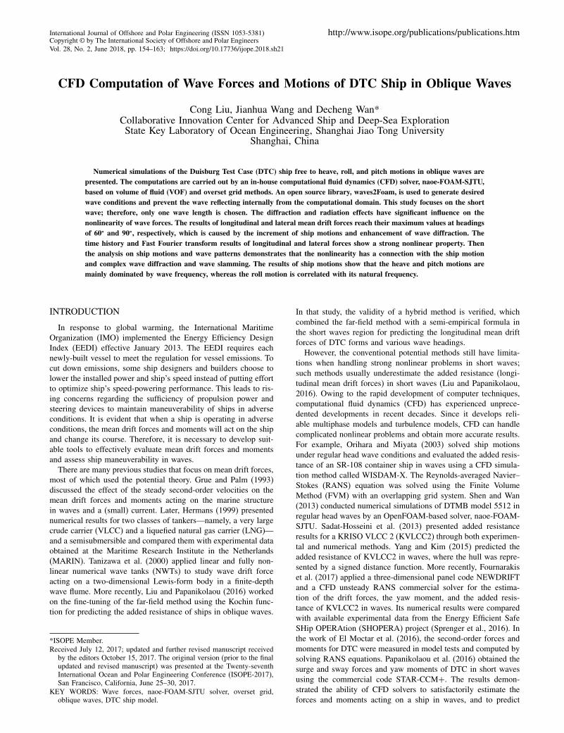
Fig. 1 Top view of the computational domain with wave genera-tion zone

In Eq. 3, Ur is the velocity field used to compress the interface,and it takes effect only on the surface interface as a result ofthe term 41 − �5�. The expression of this term can be found inBerberovic et al. (2009).

Overset Grid Technique

Overset grid is a grid system composed of multiple blocksof overlapping structured or unstructured grids. In a full oversetgrid system, a complex geometry is decomposed into a system ofgeometrically simple overlapping grids. Boundary information isexchanged between these grids via interpolation of the fluid vari-ables. In this way, the overset grid method removes the restric-tions of the mesh topology among different objects and allowsgrids to move independently within the computational domain,and it can be used to handle large-amplitude motions in the fieldof ship and ocean engineering. The most critical objective inthe overset grid is the accomplishment of information exchangebetween grid blocks. Based on the numerical methods from Open-FOAM, including the cell-centered scheme and unstructured grids,Suggar++ (Noack et al. 2009) is utilized to generate the domainconnectivity information (DCI) for the overset grid interpolationin the solver naoe-FOAM-SJTU. In this way, the solver can han-dle arbitrary motions in the simulation. For example, Wang et al.(2016a) used the same solver to simulate ship self-propulsionwith moving rudders and rotating propellers. Furthermore, Wanget al. (2016b) carried out turning circle simulation using the samesolver. In those studies, the moving rudders and rotating pro-pellers were handled by the dynamic overset grid method. Moredetails about the overset grid technique can be found in Shen et al.(2015).

Wave Generation

In general, the incoming wave is generated by imposing theboundary conditions on the tank inlet. To absorb the wave reflec-tion from the outlet, a damping zone is set at the end of the tankto avoid the wave reflection. This conventional wave generationmethod suffers reflection between the inlet and structure, espe-cially in the case free of current. One solution is to extend the dis-tance between the inlet and object. However, the disadvantage ofthis solution is the accompanying smaller time step and increasingcomputational time. To overcome this problem, the open sourcelibrary waves2Foam (Jacobsen et al., 2012) is imposed in oursolver. In the work of Jacobsen et al. (2012), a method calledthe relaxation technique is developed to achieve the functional-ity of both wave generation and absorption in a uniform way andto avoid wave reflection from the boundaries. In this study, anannular relaxation zone is set up to generate waves with different

156 CFD Computation of Wave Forces and Motions of DTC Ship in Oblique Waves

heading angles (Fig. 1). The variables �, such as U or p, insidethe relaxation zone can be expressed as follows:

�= �R�computed + 41 −�R5�target (5)

where the variable �target is a function of space and time knownfrom the Stokes wave theory, and �computed is the variable com-puted from the FVM. �R is always 1 at the interface between thenon-relaxed part of the computational domain and the relaxationzone and is 0 on the inlet boundary. And �R smoothly varies from1 to 0 in the relaxation zone. Such distribution of �R makes the �relaxed by the value of �computed and �target in the relaxation zone.In this way, the relaxation zone achieves the functionality of bothwave generation and absorption in a uniform way and avoids thewave reflection between the boundaries.

GEOMETRY AND CONDITIONS

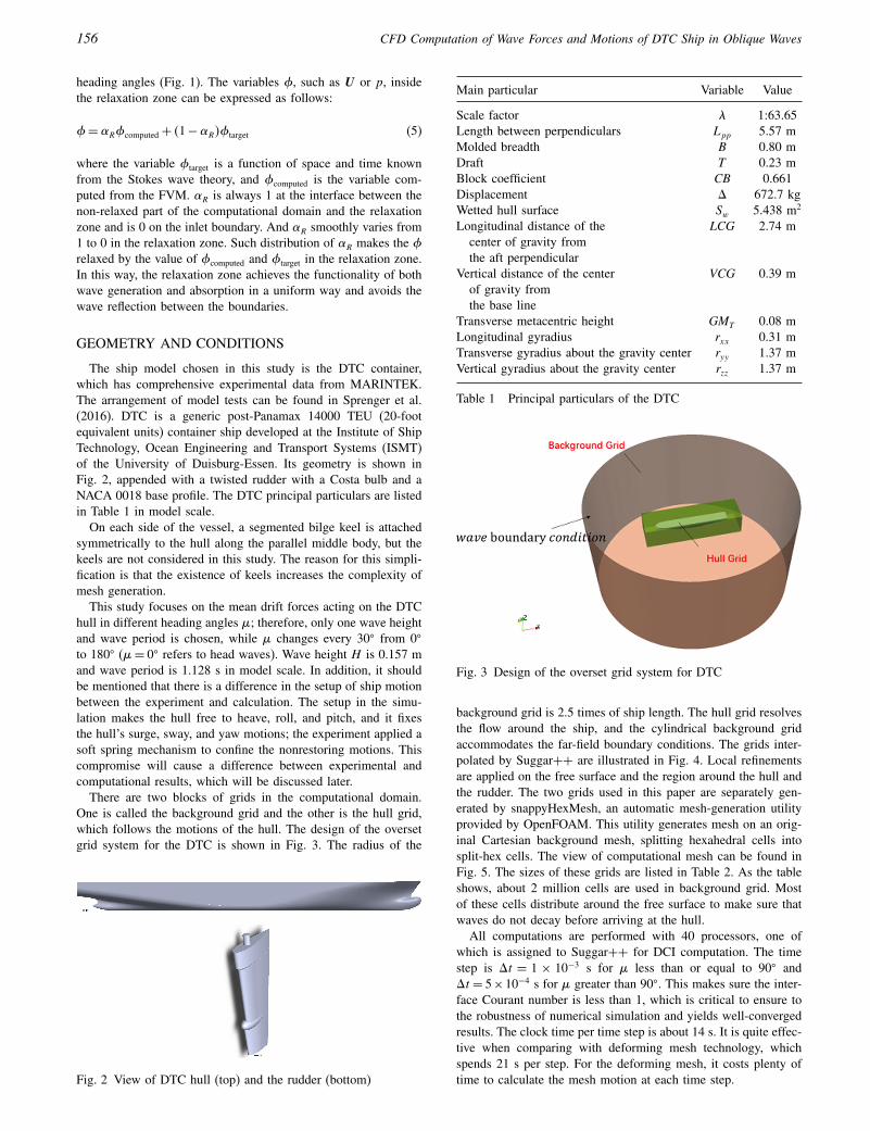
The ship model chosen in this study is the DTC container,which has comprehensive experimental data from MARINTEK.The arrangement of model tests can be found in Sprenger et al.(2016). DTC is a generic post-Panamax 14000 TEU (20-footequivalent units) container ship developed at the Institute of ShipTechnology, Ocean Engineering and Transport Systems (ISMT)of the University of Duisburg-Essen. Its geometry is shown inFig. 2, appended with a twisted rudder with a Costa bulb and aNACA 0018 base profile. The DTC principal particulars are listedin Table 1 in model scale.

On each side of the vessel, a segmented bilge keel is attachedsymmetrically to the hull along the parallel middle body, but thekeels are not considered in this study. The reason for this simpli-fication is that the existence of keels increases the complexity ofmesh generation.

This study focuses on the mean drift forces acting on the DTChull in different heading angles �; therefore, only one wave heightand wave period is chosen, while � changes every 30� from 0�

to 180� (�= 0� refers to head waves). Wave height H is 0.157 mand wave period is 1.128 s in model scale. In addition, it shouldbe mentioned that there is a difference in the setup of ship motionbetween the experiment and calculation. The setup in the simu-lation makes the hull free to heave, roll, and pitch, and it fixesthe hull’s surge, sway, and yaw motions; the experiment applied asoft spring mechanism to confine the nonrestoring motions. Thiscompromise will cause a difference between experimental andcomputational results, which will be discussed later.

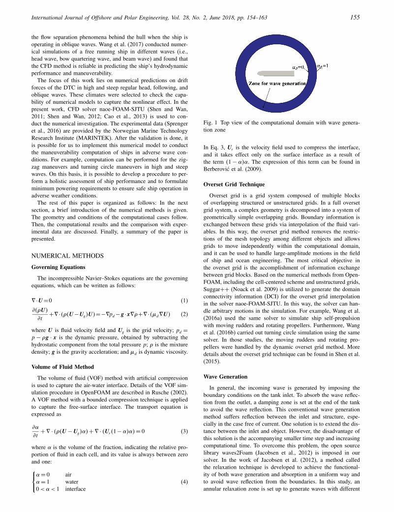
There are two blocks of grids in the computational domain.One is called the background grid and the other is the hull grid,which follows the motions of the hull. The design of the oversetgrid system for the DTC is shown in Fig. 3. The radius of the

Fig. 2 View of DTC hull (top) and the rudder (bottom)

Main particular Variable Value

Scale factor � 1:63.65Length between perpendiculars Lpp 5.57 mMolded breadth B 0.80 mDraft T 0.23 mBlock coefficient CB 0.661Displacement ã 672.7 kgWetted hull surface Sw 5.438 m2

Longitudinal distance of the LCG 2.74 mcenter of gravity fromthe aft perpendicular

Vertical distance of the center VCG 0.39 mof gravity fromthe base line

Transverse metacentric height GMT 0.08 mLongitudinal gyradius rxx 0.31 mTransverse gyradius about the gravity center ryy 1.37 mVertical gyradius about the gravity center rzz 1.37 m

Table 1 Principal particulars of the DTC

Fig. 3 Design of the overset grid system for DTC

background grid is 2.5 times of ship length. The hull grid resolvesthe flow around the ship, and the cylindrical background gridaccommodates the far-field boundary conditions. The grids inter-polated by Suggar++ are illustrated in Fig. 4. Local refinementsare applied on the free surface and the region around the hull andthe rudder. The two grids used in this paper are separately gen-erated by snappyHexMesh, an automatic mesh-generation utilityprovided by OpenFOAM. This utility generates mesh on an orig-inal Cartesian background mesh, splitting hexahedral cells intosplit-hex cells. The view of computational mesh can be found inFig. 5. The sizes of these grids are listed in Table 2. As the tableshows, about 2 million cells are used in background grid. Mostof these cells distribute around the free surface to make sure thatwaves do not decay before arriving at the hull.

All computations are performed with 40 processors, one ofwhich is assigned to Suggar++ for DCI computation. The timestep is ãt = 1 × 10−3 s for � less than or equal to 90� andãt = 5×10−4 s for � greater than 90�. This makes sure the inter-face Courant number is less than 1, which is critical to ensure tothe robustness of numerical simulation and yields well-convergedresults. The clock time per time step is about 14 s. It is quite effec-tive when comparing with deforming mesh technology, whichspends 21 s per step. For the deforming mesh, it costs plenty oftime to calculate the mesh motion at each time step.

International Journal of Offshore and Polar Engineering, Vol. 28, No. 2, June 2018, pp. 154–163 157

Fig. 4 Mesh views for vertical plane at y = 0 (red for backgroundmesh and green for hull mesh)

(a) Global mesh (split along central fore-and-aft vertical plane)

(b) Local mesh (Bow) (c) Local mesh (Stern)

Fig. 5 Computational mesh

Hull Background Total

Number of cells 1,461,919 2,226,624 3,688,543

Table 2 Grid sizes for computations of mean drift forces in reg-ular waves

RESULTS

Mean Drift Forces in Regular Waves

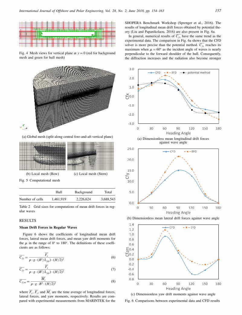
Figure 6 shows the coefficients of longitudinal mean driftforces, lateral mean drift forces, and mean yaw drift moments forthe � in the range of 0� to 180�. The definitions of these coeffi-cients are as follows:

Cfx =Fx

� · g · 4B2/Lpp5 · 4H/252(6)

Cfy =Fx

� · g · 4B2/Lpp5 · 4H/252(7)

Cfzm =Mz

� · g ·B2 · 4H/252(8)

where Fx, Fy , and Mz are the time average of longitudinal forces,lateral forces, and yaw moments, respectively. Results are com-pared with experimental measurements from MARINTEK for the

SHOPERA Benchmark Workshop (Sprenger et al., 2016). Theresults of longitudinal mean drift forces obtained by potential the-ory (Liu and Papanikolaou, 2016) are also present in Fig. 6a.

In general, numerical results of Cfx have the same trend as theexperimental data. The comparison in Fig. 6a shows that the CFDsolver is more precise than the potential method. Cfx reaches itsmaximum when �= 60� as the incident angle of waves is nearlyperpendicular to the forward shoulder of the hull. Consequently,the diffraction increases and the radiation also become stronger

(a) Dimensionless mean longitudinal drift forcesagainst wave angle

(b) Dimensionless mean lateral drift forces against wave angle

(c) Dimensionless yaw drift moments against wave angle

Fig. 6 Comparisons between experimental data and CFD results

158 CFD Computation of Wave Forces and Motions of DTC Ship in Oblique Waves

(a) Time history of Cfx and Cfy for �= 0� (b) Time history of Cfx and Cfy for �= 30�

(c) Time history of Cfx and Cfy for �= 60� (d) Time history of Cfx and Cfy for �= 90�

(e) Time history of Cfx and Cfy for �= 120� (f) Time history of Cfx and Cfy for �= 150�

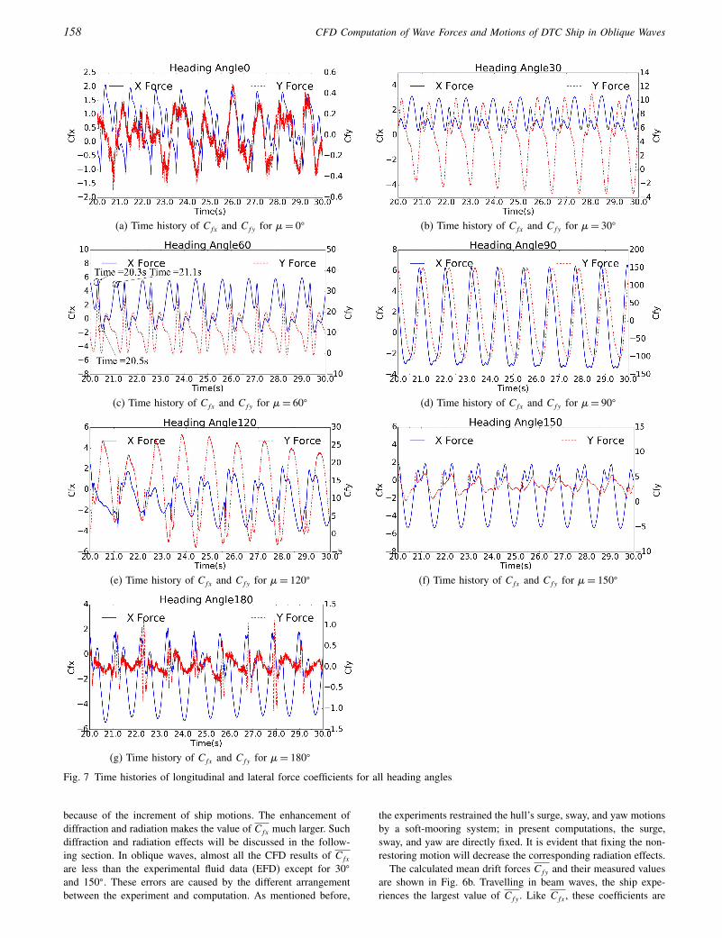
(g) Time history of Cfx and Cfy for �= 180�

Fig. 7 Time histories of longitudinal and lateral force coefficients for all heading angles

because of the increment of ship motions. The enhancement ofdiffraction and radiation makes the value of Cfx much larger. Suchdiffraction and radiation effects will be discussed in the follow-ing section. In oblique waves, almost all the CFD results of Cfx

are less than the experimental fluid data (EFD) except for 30�

and 150�. These errors are caused by the different arrangementbetween the experiment and computation. As mentioned before,

the experiments restrained the hull’s surge, sway, and yaw motionsby a soft-mooring system; in present computations, the surge,sway, and yaw are directly fixed. It is evident that fixing the non-restoring motion will decrease the corresponding radiation effects.

The calculated mean drift forces Cfy and their measured valuesare shown in Fig. 6b. Travelling in beam waves, the ship expe-riences the largest value of Cfy . Like Cfx, these coefficients are

International Journal of Offshore and Polar Engineering, Vol. 28, No. 2, June 2018, pp. 154–163 159

underestimated by CFD, especially for the beam waves, whichis underestimated by 27.6%. The errors of CFD predictions forCfy under other wave conditions vary from 10.2% to 25.2%. Inthe oblique wave, the second-order force is dependent on motion,particularly on the sway motion in the beam waves. Thus, fixingthe non-restoring motion will arise the drift force error relatedto the radiation especially when � is close to 90�. Consequently,the difference in Cfy between CFD and EFD increases as � isapproaching 90� (as shown in Fig. 6b).

The comparison of mean yaw drift forces Cfzm is shown inFig. 6c. It shows good agreement between CFD and EFD when� < 90�. The largest value of yaw drift force occurs when � =

60�, since Cfx reaches its maximum value and the arm of forceis quite considerable. Similar to Cfx, the yaw moment for 60� isunderestimated. The results of Cfzm have only the same trend withEFD results, and errors are obvious in some cases.

Time History of Forces

The time histories of force coefficients, Cfx and Cfy , can bedefined in the same way as Cfx and Cfy by using transient val-ues. The results of Cfx and Cfy for all cases can be found inFig. 7. The results present strong nonlinear behaviors instead ofsmooth cosine curves. As shown in Fig. 7c, the extremum ofCfx appears three times in one period, indicating that this curveis composed of several different frequency components. For thecases of 0� (Fig. 7a), 120� (Fig. 7e), and 180� (Fig. 7g), spikescan be observed corresponding to strong wave slamming. Withthe heading approaching 90�, the amplitudes of both Cfx and Cfy

increase. The peak values of Cfx increase moderately and are of

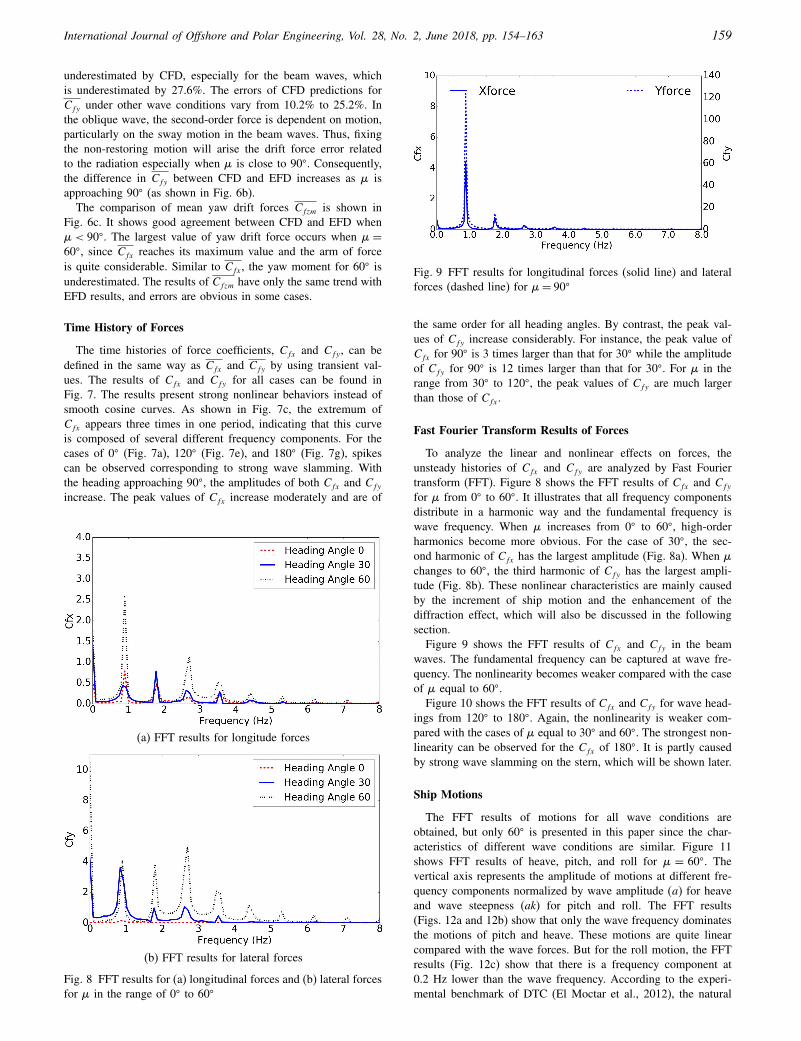
(a) FFT results for longitude forces

(b) FFT results for lateral forces

Fig. 8 FFT results for (a) longitudinal forces and (b) lateral forcesfor � in the range of 0� to 60�

Fig. 9 FFT results for longitudinal forces (solid line) and lateralforces (dashed line) for �= 90�

the same order for all heading angles. By contrast, the peak val-ues of Cfy increase considerably. For instance, the peak value ofCfx for 90� is 3 times larger than that for 30� while the amplitudeof Cfy for 90� is 12 times larger than that for 30�. For � in therange from 30� to 120�, the peak values of Cfy are much largerthan those of Cfx.

Fast Fourier Transform Results of Forces

To analyze the linear and nonlinear effects on forces, theunsteady histories of Cfx and Cfy are analyzed by Fast Fouriertransform (FFT). Figure 8 shows the FFT results of Cfx and Cfy

for � from 0� to 60�. It illustrates that all frequency componentsdistribute in a harmonic way and the fundamental frequency iswave frequency. When � increases from 0� to 60�, high-orderharmonics become more obvious. For the case of 30�, the sec-ond harmonic of Cfx has the largest amplitude (Fig. 8a). When �

changes to 60�, the third harmonic of Cfy has the largest ampli-tude (Fig. 8b). These nonlinear characteristics are mainly causedby the increment of ship motion and the enhancement of thediffraction effect, which will also be discussed in the followingsection.

Figure 9 shows the FFT results of Cfx and Cfy in the beamwaves. The fundamental frequency can be captured at wave fre-quency. The nonlinearity becomes weaker compared with the caseof � equal to 60�.

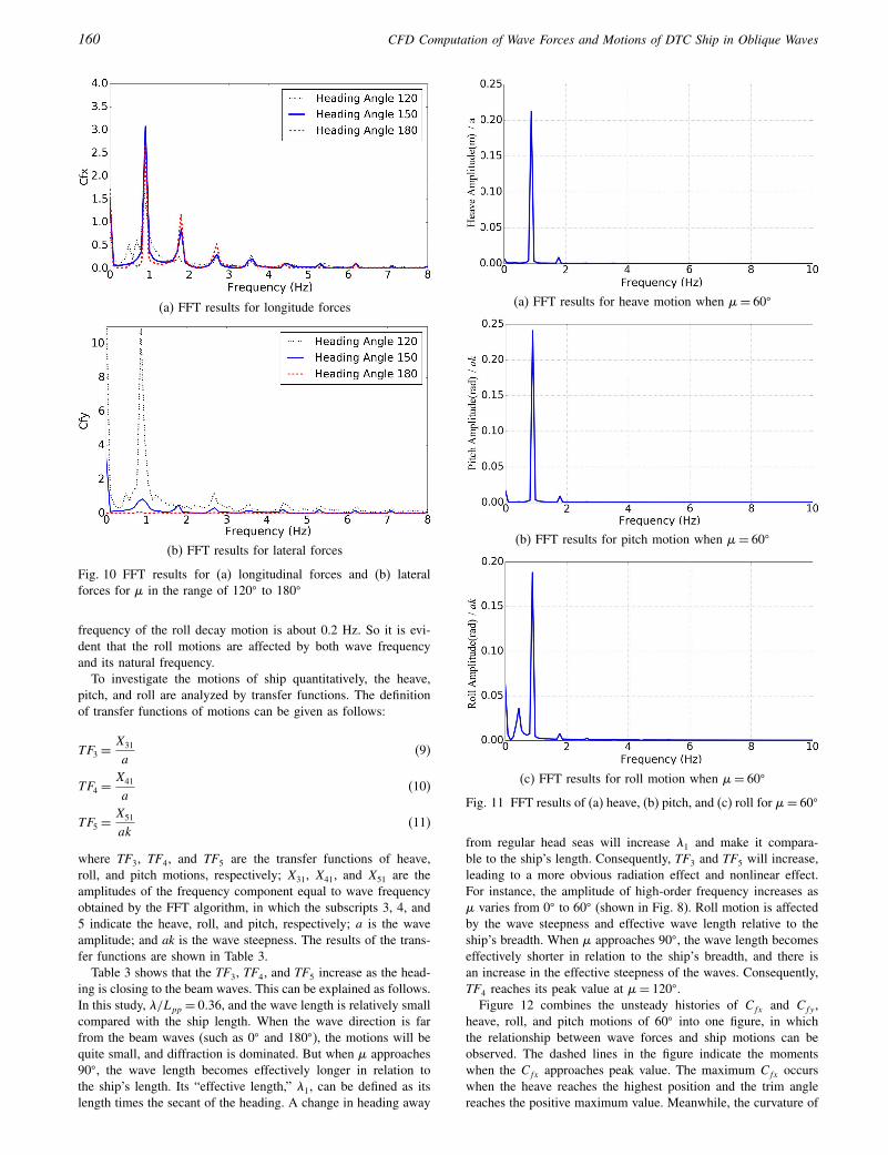
Figure 10 shows the FFT results of Cfx and Cfy for wave head-ings from 120� to 180�. Again, the nonlinearity is weaker com-pared with the cases of � equal to 30� and 60�. The strongest non-linearity can be observed for the Cfx of 180�. It is partly causedby strong wave slamming on the stern, which will be shown later.

Ship Motions

The FFT results of motions for all wave conditions areobtained, but only 60� is presented in this paper since the char-acteristics of different wave conditions are similar. Figure 11shows FFT results of heave, pitch, and roll for � = 60�. Thevertical axis represents the amplitude of motions at different fre-quency components normalized by wave amplitude (a) for heaveand wave steepness (ak) for pitch and roll. The FFT results(Figs. 12a and 12b) show that only the wave frequency dominatesthe motions of pitch and heave. These motions are quite linearcompared with the wave forces. But for the roll motion, the FFTresults (Fig. 12c) show that there is a frequency component at0.2 Hz lower than the wave frequency. According to the experi-mental benchmark of DTC (El Moctar et al., 2012), the natural

160 CFD Computation of Wave Forces and Motions of DTC Ship in Oblique Waves

(a) FFT results for longitude forces

(b) FFT results for lateral forces

Fig. 10 FFT results for (a) longitudinal forces and (b) lateralforces for � in the range of 120� to 180�

frequency of the roll decay motion is about 0.2 Hz. So it is evi-dent that the roll motions are affected by both wave frequencyand its natural frequency.

To investigate the motions of ship quantitatively, the heave,pitch, and roll are analyzed by transfer functions. The definitionof transfer functions of motions can be given as follows:

TF3 =X31

a(9)

TF4 =X41

a(10)

TF5 =X51

ak(11)

where TF3, TF4, and TF5 are the transfer functions of heave,roll, and pitch motions, respectively; X31, X41, and X51 are theamplitudes of the frequency component equal to wave frequencyobtained by the FFT algorithm, in which the subscripts 3, 4, and5 indicate the heave, roll, and pitch, respectively; a is the waveamplitude; and ak is the wave steepness. The results of the trans-fer functions are shown in Table 3.

Table 3 shows that the TF3, TF4, and TF5 increase as the head-ing is closing to the beam waves. This can be explained as follows.In this study, �/Lpp = 0036, and the wave length is relatively smallcompared with the ship length. When the wave direction is farfrom the beam waves (such as 0� and 180�), the motions will bequite small, and diffraction is dominated. But when � approaches90�, the wave length becomes effectively longer in relation tothe ship’s length. Its “effective length,” �1, can be defined as itslength times the secant of the heading. A change in heading away

(a) FFT results for heave motion when �= 60�

(b) FFT results for pitch motion when �= 60�

(c) FFT results for roll motion when �= 60�

Fig. 11 FFT results of (a) heave, (b) pitch, and (c) roll for �= 60�

from regular head seas will increase �1 and make it compara-ble to the ship’s length. Consequently, TF3 and TF5 will increase,leading to a more obvious radiation effect and nonlinear effect.For instance, the amplitude of high-order frequency increases as� varies from 0� to 60� (shown in Fig. 8). Roll motion is affectedby the wave steepness and effective wave length relative to theship’s breadth. When � approaches 90�, the wave length becomeseffectively shorter in relation to the ship’s breadth, and there isan increase in the effective steepness of the waves. Consequently,TF4 reaches its peak value at �= 120�.

Figure 12 combines the unsteady histories of Cfx and Cfy ,heave, roll, and pitch motions of 60� into one figure, in whichthe relationship between wave forces and ship motions can beobserved. The dashed lines in the figure indicate the momentswhen the Cfx approaches peak value. The maximum Cfx occurswhen the heave reaches the highest position and the trim anglereaches the positive maximum value. Meanwhile, the curvature of

International Journal of Offshore and Polar Engineering, Vol. 28, No. 2, June 2018, pp. 154–163 161

Fig. 12 Time histories of Cfx, Cfy , heave, roll, and pitch (� =

60�)

Heading angles 0 30 60 90 120 150 180

TF3 0.087 0.123 0.212 0.679 0.177 0.067 0.07TF4 0 0.145 0.188 0.234 0.312 0.066 0TF5 0.111 0.151 0.241 0.037 0.095 0.117 0.083

Table 3 Transfer functions of heave and pitch motions

Cfy also changes at this moment. In addition, the minimum Cfx

and Cfy occur when the heave and pitch approach negative max-imum values. Therefore, the ship motions have an impact on theforces and do contribute to the nonlinearity.

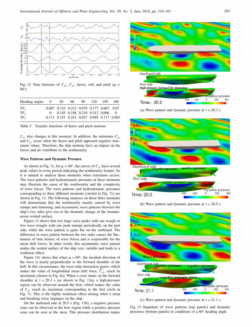
Wave Patterns and Dynamic Pressure

As shown in Fig. 7c, for �= 60�, the curves of Cfx have severalpeak values in every period indicating the nonlinearity feature. Soit is natural to analyze these moments when extremum occurs.The wave patterns and hydrodynamic pressures at these momentsmay illustrate the cause of the nonlinearity and the complexityof wave forces. The wave patterns and hydrodynamic pressurescorresponding to three different moments (circled in Fig. 7c) areshown in Fig. 13. The following analyses on these three momentswill demonstrate that the nonlinearity mainly caused by waverunups and slamming, and asymmetric wave patterns between theship’s two sides give rise to the dramatic change of the instanta-neous wetted surface.

Figure 13 shows that two large wave peaks with one trough ortwo wave troughs with one peak emerge periodically on the portside, while the wave pattern is quite flat on the starboard. Thedifference in wave pattern between the two sides causes the fluc-tuation of time history of wave forces and is responsible for themean drift forces. In other words, this asymmetric wave patternmakes the wetted surface of the ship very variable and leads to anonlinear effect.

Figure 13c shows that when �= 60�, the incident direction ofthe wave is nearly perpendicular to the forward shoulder of thehull. In this circumstance, the wave-ship interaction grows, whichmakes the value of longitudinal mean drift force, Cfx, reach itsmaximum (shown in Fig. 6a). When a crest slams on the forwardshoulder at t = 2003 s (as shown in Fig. 13a), a high-pressureregion can be observed around the bow, which makes the valueof Cfx reach its maximum corresponding to the first circle inFig. 7c. This is the highly nonlinear effect arising when a steepand breaking wave impinges on the ship.

On the starboard side at 20.5 s (Fig. 13b), a negative pressurezone can be observed at the bow region while a positive pressurezone can be seen at the stern. This pressure distribution makes

(a) Wave pattern and dynamic pressure at t = 2003 s

(b) Wave pattern and dynamic pressure at t = 2005 s

(c) Wave pattern and dynamic pressure at t = 2101 s

Fig. 13 Snapshots of wave patterns (top panels) and dynamicpressures (bottom panels) in conditions of a 60� heading angle

162 CFD Computation of Wave Forces and Motions of DTC Ship in Oblique Waves

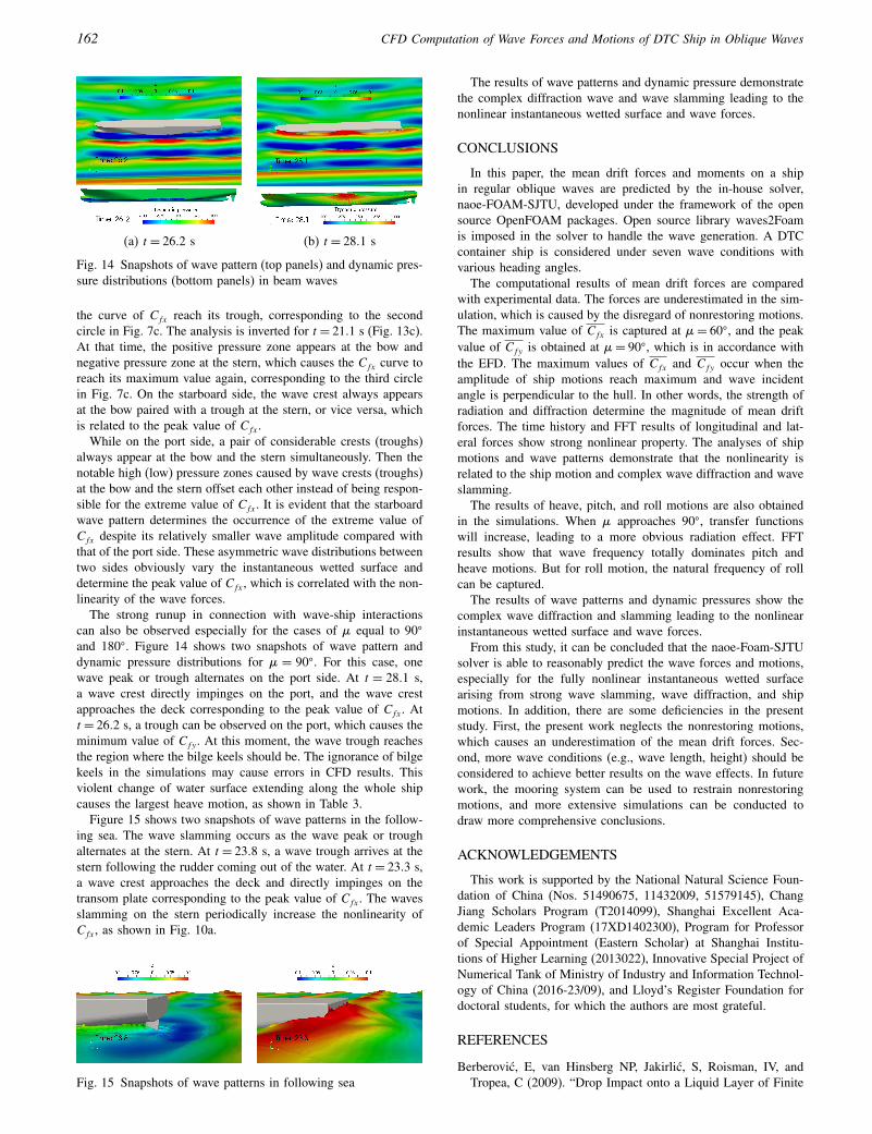
(a) t = 2602 s (b) t = 2801 s

Fig. 14 Snapshots of wave pattern (top panels) and dynamic pres-sure distributions (bottom panels) in beam waves

the curve of Cfx reach its trough, corresponding to the secondcircle in Fig. 7c. The analysis is inverted for t = 2101 s (Fig. 13c).At that time, the positive pressure zone appears at the bow andnegative pressure zone at the stern, which causes the Cfx curve toreach its maximum value again, corresponding to the third circlein Fig. 7c. On the starboard side, the wave crest always appearsat the bow paired with a trough at the stern, or vice versa, whichis related to the peak value of Cfx.

While on the port side, a pair of considerable crests (troughs)always appear at the bow and the stern simultaneously. Then thenotable high (low) pressure zones caused by wave crests (troughs)at the bow and the stern offset each other instead of being respon-sible for the extreme value of Cfx. It is evident that the starboardwave pattern determines the occurrence of the extreme value ofCfx despite its relatively smaller wave amplitude compared withthat of the port side. These asymmetric wave distributions betweentwo sides obviously vary the instantaneous wetted surface anddetermine the peak value of Cfx, which is correlated with the non-linearity of the wave forces.

The strong runup in connection with wave-ship interactionscan also be observed especially for the cases of � equal to 90�

and 180�. Figure 14 shows two snapshots of wave pattern anddynamic pressure distributions for � = 90�. For this case, onewave peak or trough alternates on the port side. At t = 2801 s,a wave crest directly impinges on the port, and the wave crestapproaches the deck corresponding to the peak value of Cfx. Att = 2602 s, a trough can be observed on the port, which causes theminimum value of Cfy . At this moment, the wave trough reachesthe region where the bilge keels should be. The ignorance of bilgekeels in the simulations may cause errors in CFD results. Thisviolent change of water surface extending along the whole shipcauses the largest heave motion, as shown in Table 3.

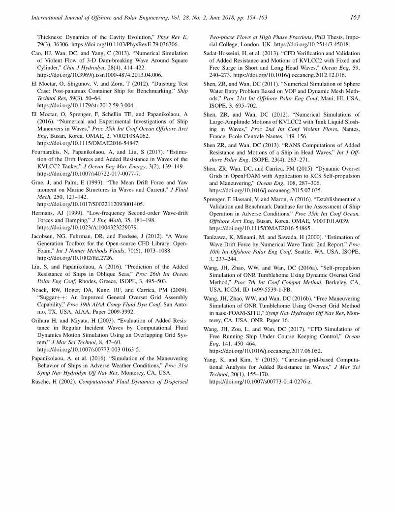
Figure 15 shows two snapshots of wave patterns in the follow-ing sea. The wave slamming occurs as the wave peak or troughalternates at the stern. At t = 2308 s, a wave trough arrives at thestern following the rudder coming out of the water. At t = 2303 s,a wave crest approaches the deck and directly impinges on thetransom plate corresponding to the peak value of Cfx. The wavesslamming on the stern periodically increase the nonlinearity ofCfx, as shown in Fig. 10a.

Fig. 15 Snapshots of wave patterns in following sea

The results of wave patterns and dynamic pressure demonstratethe complex diffraction wave and wave slamming leading to thenonlinear instantaneous wetted surface and wave forces.

CONCLUSIONS

In this paper, the mean drift forces and moments on a shipin regular oblique waves are predicted by the in-house solver,naoe-FOAM-SJTU, developed under the framework of the opensource OpenFOAM packages. Open source library waves2Foamis imposed in the solver to handle the wave generation. A DTCcontainer ship is considered under seven wave conditions withvarious heading angles.

The computational results of mean drift forces are comparedwith experimental data. The forces are underestimated in the sim-ulation, which is caused by the disregard of nonrestoring motions.The maximum value of Cfx is captured at �= 60�, and the peakvalue of Cfy is obtained at �= 90�, which is in accordance withthe EFD. The maximum values of Cfx and Cfy occur when theamplitude of ship motions reach maximum and wave incidentangle is perpendicular to the hull. In other words, the strength ofradiation and diffraction determine the magnitude of mean driftforces. The time history and FFT results of longitudinal and lat-eral forces show strong nonlinear property. The analyses of shipmotions and wave patterns demonstrate that the nonlinearity isrelated to the ship motion and complex wave diffraction and waveslamming.

The results of heave, pitch, and roll motions are also obtainedin the simulations. When � approaches 90�, transfer functionswill increase, leading to a more obvious radiation effect. FFTresults show that wave frequency totally dominates pitch andheave motions. But for roll motion, the natural frequency of rollcan be captured.

The results of wave patterns and dynamic pressures show thecomplex wave diffraction and slamming leading to the nonlinearinstantaneous wetted surface and wave forces.

From this study, it can be concluded that the naoe-Foam-SJTUsolver is able to reasonably predict the wave forces and motions,especially for the fully nonlinear instantaneous wetted surfacearising from strong wave slamming, wave diffraction, and shipmotions. In addition, there are some deficiencies in the presentstudy. First, the present work neglects the nonrestoring motions,which causes an underestimation of the mean drift forces. Sec-ond, more wave conditions (e.g., wave length, height) should beconsidered to achieve better results on the wave effects. In futurework, the mooring system can be used to restrain nonrestoringmotions, and more extensive simulations can be conducted todraw more comprehensive conclusions.

ACKNOWLEDGEMENTS

This work is supported by the National Natural Science Foun-dation of China (Nos. 51490675, 11432009, 51579145), ChangJiang Scholars Program (T2014099), Shanghai Excellent Aca-demic Leaders Program (17XD1402300), Program for Professorof Special Appointment (Eastern Scholar) at Shanghai Institu-tions of Higher Learning (2013022), Innovative Special Project ofNumerical Tank of Ministry of Industry and Information Technol-ogy of China (2016-23/09), and Lloyd’s Register Foundation fordoctoral students, for which the authors are most grateful.

REFERENCES

Berberovic, E, van Hinsberg NP, Jakirlic, S, Roisman, IV, andTropea, C (2009). “Drop Impact onto a Liquid Layer of Finite

International Journal of Offshore and Polar Engineering, Vol. 28, No. 2, June 2018, pp. 154–163 163

Thickness: Dynamics of the Cavity Evolution,” Phys Rev E,79(3), 36306. https://doi.org/10.1103/PhysRevE.79.036306.

Cao, HJ, Wan, DC, and Yang, C (2013). “Numerical Simulationof Violent Flow of 3-D Dam-breaking Wave Around SquareCylinder,” Chin J Hydrodyn, 28(4), 414–422.https://doi.org/10.3969/j.issn1000-4874.2013.04.006.

El Moctar, O, Shigunov, V, and Zorn, T (2012). “Duisburg TestCase: Post-panamax Container Ship for Benchmarking,” ShipTechnol Res, 59(3), 50–64.https://doi.org/10.1179/str.2012.59.3.004.

El Moctar, O, Sprenger, F, Schellin TE, and Papanikolaou, A(2016). “Numerical and Experimental Investigations of ShipManeuvers in Waves,” Proc 35th Int Conf Ocean Offshore ArctEng, Busan, Korea, OMAE, 2, V002T08A062.https://doi.org/10.1115/OMAE2016-54847.

Fournarakis, N, Papanikolaou, A, and Liu, S (2017). “Estima-tion of the Drift Forces and Added Resistance in Waves of theKVLCC2 Tanker,” J Ocean Eng Mar Energy, 3(2), 139–149.https://doi.org/10.1007/s40722-017-0077-7.

Grue, J, and Palm, E (1993). “The Mean Drift Force and Yawmoment on Marine Structures in Waves and Current,” J FluidMech, 250, 121–142.https://doi.org/10.1017/S0022112093001405.

Hermans, AJ (1999). “Low-frequency Second-order Wave-driftForces and Damping,” J Eng Math, 35, 181–198.https://doi.org/10.1023/A:1004323229079.

Jacobsen, NG, Fuhrman, DR, and Fredsøe, J (2012). “A WaveGeneration Toolbox for the Open-source CFD Library: Open-Foam,” Int J Numer Methods Fluids, 70(6), 1073–1088.https://doi.org/10.1002/fld.2726.

Liu, S, and Papanikolaou, A (2016). “Prediction of the AddedResistance of Ships in Oblique Seas,” Proc 26th Int OceanPolar Eng Conf, Rhodes, Greece, ISOPE, 3, 495–503.

Noack, RW, Boger, DA, Kunz, RF, and Carrica, PM (2009).“Suggar++: An Improved General Overset Grid AssemblyCapability,” Proc 19th AIAA Comp Fluid Dyn Conf, San Anto-nio, TX, USA, AIAA, Paper 2009-3992.

Orihara H, and Miyata, H (2003). “Evaluation of Added Resis-tance in Regular Incident Waves by Computational FluidDynamics Motion Simulation Using an Overlapping Grid Sys-tem,” J Mar Sci Technol, 8, 47–60.https://doi.org/10.1007/s00773-003-0163-5.

Papanikolaou, A, et al. (2016). “Simulation of the ManeuveringBehavior of Ships in Adverse Weather Conditions,” Proc 31stSymp Nav Hydrodyn Off Nav Res, Monterey, CA, USA.

Rusche, H (2002). Computational Fluid Dynamics of Dispersed

Two-phase Flows at High Phase Fractions, PhD Thesis, Impe-rial College, London, UK. https://doi.org/10.2514/3.45018.

Sadat-Hosseini, H, et al. (2013). “CFD Verification and Validationof Added Resistance and Motions of KVLCC2 with Fixed andFree Surge in Short and Long Head Waves,” Ocean Eng, 59,240–273. https://doi.org/10.1016/j.oceaneng.2012.12.016.

Shen, ZR, and Wan, DC (2011). “Numerical Simulation of SphereWater Entry Problem Based on VOF and Dynamic Mesh Meth-ods,” Proc 21st Int Offshore Polar Eng Conf, Maui, HI, USA,ISOPE, 3, 695–702.

Shen, ZR, and Wan, DC (2012). “Numerical Simulations ofLarge-Amplitude Motions of KVLCC2 with Tank Liquid Slosh-ing in Waves,” Proc 2nd Int Conf Violent Flows, Nantes,France, Ecole Centrale Nantes, 149–156.

Shen ZR, and Wan, DC (2013). “RANS Computations of AddedResistance and Motions of a Ship in Head Waves,” Int J Off-shore Polar Eng, ISOPE, 23(4), 263–271.

Shen, ZR, Wan, DC, and Carrica, PM (2015). “Dynamic OversetGrids in OpenFOAM with Application to KCS Self-propulsionand Maneuvering,” Ocean Eng, 108, 287–306.https://doi.org/10.1016/j.oceaneng.2015.07.035.

Sprenger, F, Hassani, V, and Maron, A (2016). “Establishment of aValidation and Benchmark Database for the Assessment of ShipOperation in Adverse Conditions,” Proc 35th Int Conf Ocean,Offshore Arct Eng, Busan, Korea, OMAE, V001T01A039.https://doi.org/10.1115/OMAE2016-54865.

Tanizawa, K, Minami, M, and Sawada, H (2000). “Estimation ofWave Drift Force by Numerical Wave Tank: 2nd Report,” Proc10th Int Offshore Polar Eng Conf, Seattle, WA, USA, ISOPE,3, 237–244.

Wang, JH, Zhao, WW, and Wan, DC (2016a). “Self-propulsionSimulation of ONR Tumblehome Using Dynamic Overset GridMethod,” Proc 7th Int Conf Comput Method, Berkeley, CA,USA, ICCM, ID 1499-5539-1-PB.

Wang, JH, Zhao, WW, and Wan, DC (2016b). “Free ManeuveringSimulation of ONR Tumblehome Using Overset Grid Methodin naoe-FOAM-SJTU,” Symp Nav Hydrodyn Off Nav Res, Mon-terey, CA, USA, ONR, Paper 16.

Wang, JH, Zou, L, and Wan, DC (2017). “CFD Simulations ofFree Running Ship Under Course Keeping Control,” OceanEng, 141, 450–464.https://doi.org/10.1016/j.oceaneng.2017.06.052.

Yang, K, and Kim, Y (2015). “Cartesian-grid-based Computa-tional Analysis for Added Resistance in Waves,” J Mar SciTechnol, 20(1), 155–170.https://doi.org/10.1007/s00773-014-0276-z.