CFD Analysis of the Electrostatic Spray Painting Process ... M2-B-3.pdf · ILASS Americas, 21 st Annual Conference on Liquid Atomization and Spray Systems, Orlando, Florida, USA,

ILASS Americas, 21st Annual Conference on Liquid Atomization and Spray Systems, Orlando, Florida, USA, May 2008

CFD Analysis of the Electrostatic Spray Painting Process with a Rotating Bell Cup

V. Viti *, J. Kulkarni

Ansys, Inc., 10 Cavendish Ct., Lebanon, NH 03766, USA

A. Watve

ANSYS Fluent India Pvt. Ltd, Pune Infotech Park, Pune, India

Abstract

The use of electrostatic fields in the spray painting process is a common technique utilized to increase the transfer efficiency of the process and the quality of the applied coating. The electrostatic field is usually generated by apply-ing a voltage differential between the spray gun and the grounded target surface so that the electric potential will drive the charged droplets toward the target. In modern booths the coatings are often applied via rotating-cup-type spray guns mounted on automated robotic arms that move along pre-programmed trajectories. In such systems the paint droplets are generated by atomization of the thin film of paint that covers the surface of the rotating cup when it hits the serrated cup rim. The so-formed droplets are charged with the same potential polarity as the spray gun via induction or corona charging and are pushed by the electrostatic force toward the grounded target surface. In addi-tion to the electrostatic force, a strong airflow coaxial with the spray gun, referred to as “shaping air”, helps convec-tion of the droplets toward the target. Typically this process occurs in a painting booth where for safety reasons and according to regulations a strong crossflow of air-conditioned air exists. The interaction of these three forces as well as the particle size determines the path that the droplets will follow and ultimately the location of their deposition. While the general characteristics of the electrostatic spray painting process (ESP) process are well understood, there is a lack of detailed physical analysis which is essential for the optimization of the process. The present work makes use of Computational Fluid Dynamics (CFD) methods to analyze the interaction of the flowfield with the electro-static field and the effect that their coupling has on the paint droplets. While the flowfield and the electrostatic field are computed using an Eulerian approach through the use of a finite-volume formulation, the droplet trajectory is computed using a Lagrangean scheme that tracks each particle trajectory by integrating its equation of motion. The paint droplets have an initial size distribution determined by experiment and their initial specific electrostatic charge is calculated following empirical correlations and basic principles. The coupling between the flowfield and the elec-trostatic field is given by the computed particle trajectories since the motion of the particle is affected both by the flowfield and the electrostatic field and in turn, the electrostatic field is affected by the particle motion via the space charge. Flow turbulence effects are computed using the realizable k-ε model and particle turbulent dispersion is computed using a random-walk approach. The CFD commercial code FLUENT was used to perform these simula-tions since the off-the-shelf code is capable of simulating the flowfield and the electrostatic field as well as the parti-cle trajectories. In addition to these standard models, specific subroutines were written to compute the interaction of the droplets with the electrostatic field via the space charge. A graphic-user interface was developed in order to make the setup of these simulations faster and more consistent so that a high degree of repeatability can be achieved. The present paper is a summary of the ongoing work being performed in this area at the Lebanon Ansys office.

*Corresponding author, Consulting Engineer, [email protected], +1 (603) 643 2600

2

Introduction The application of electrostatic fields to the coating

process is a very well-established technique in the manufacturing industry. While the general workings of the process are well-understood, there still is a lack of deep insight of i) all of the physical processes that take part in the deposition and, especially, ii) how these processes interact with one another. The understanding of the physics and their interaction is relevant for the optimization of the coating process. Till now this has been primarily fine-tuned at the system level by analyz-ing bulk parameters via experimental methods and em-pirical correlations and then make changes at the sys-tem level. However, the non-linearity of the interactions makes the problem difficult to treat, especially when the process has already been extensively improved em-pirically and when there is the need to perform the op-timization of sensitive parameters such as the film thickness and the coating quality.

In the present work we are concerned with the elec-

trostatic spray painting (ESP) process using either sol-vent or water-based liquid paint. The ESP process can be divided into four different sub-processes depending on what physics are locally dominant [1][2]; the atomi-zation, the droplet charging, the transport and deposi-tion. The analysis and the control of each of these proc-esses presents several challenges and the detailed phys-ics are still unknown and are the subject of intense re-search [2]. Due to its complexity, atomization of liquid jets and films is a very active field in which researchers are performing theoretical, experimental and numerical work to better understand the different breakup mecha-nisms that interact to produce sprays [1]-[10]. The work performed by Kazama [11] clearly shows the complex-ity of the atomization when applied to the ESP problem with a rotating cup. We are not attempting to simulate atomization, thus the initial particle size distribution is taken from experimental measurements and it is repre-sentative of the distribution function produced by rotat-ing cups with a serrated rim under normal operating conditions [1]. Also, droplet dynamics during deposi-tion are not treated, and we are assuming that all of the droplets that reach the target are deposited at that loca-tion without splashing, the focus of the paper being, partly the charging of the droplet and mainly the trans-port mechanisms.

The transport problem has been studied by several

researchers since it appears that, at the current state, most benefits are to be derived by focusing on its opti-mization. Also, with the exception of selected physics, the transport process is essentially the same for ESP and powder coating systems and for completeness we

include several references to research work in powder coating.

Hackberg et al.13 studied the problem using an axi-

symmetric flow and a simple Stoke’s law flow model to compute the trajectory of the paint particles. Their re-sults showed the usefulness of numerical simulations in predicting the trends in the painting process. Ellwood et al. [14] performed numerical simulations of a station-ary, axis-symmetric, vertical paint gun. In their model the flow was assumed to be laminar and axi-symmetric. The cup was stationary and not rotating, the booth air-flow was co-axial to the gun and gravity was not in-cluded. The simulations included the coupling of the flowfield with the electrostatic field, and the effect of the paint particles on the continuous phase. They showed that the space charge has a considerable impact on the particle trajectories thus strongly influencing the results. The coupling of the particles with the continu-ous phase was found to be important only in the region near the injection locations where the concentration of paint particles is highest. Bottner and Sommerfeld [15] performed simulations of the powder coating process in a turbulent flow using a finite-volume code, FAST, and included both the first Maxwell equation (Poisson equa-tion) and the continuity of current equation. However, their film-thickness results did not match favorably with the experimental measurements and the authors attributed the disagreement to the complexity of the flowfield created by the round nozzle with a dispersion cone. Miller et al. [16] simulated the flowfield in a paint booth using particle-collision techniques. They assumed no momentum coupling between the paint particles and the flowfield and did not include the effect of a space charge. They analyzed qualitatively the effect of the shaping air velocity, of the cup rotational speed and of the charge-to-mass ratio of the particles. Their simula-tions showed that there is little influence of the shaping air flow on the transfer efficiency. On the other hand, they showed that the scatter of the paint particles in-creased with the rotational speed of the cup and that the effect of an increase of charge-to-mass ratio is equiva-lent to an increase in the electrostatic field. Su-Im et al. [17] conducted a numerical study of the transport phe-nomenon for a rotary bell paint spray. Similarly to Ell-wood et al., they considered the momentum coupling of the particles with the flowfield. However, the electro-static field was not computed numerically but rather it was derived analytically. As expected, it was concluded that the transfer efficiency increases with charge-to-mass ratio. Also, they found that transfer efficiency increases with the shaping air flow, up to a maximum value at which the transfer efficiency and shaping air flow become inversely proportional.

3

Extensive CFD simulations have been performed for the powder coating process. Researchers at the Fraunhofer Institute in Germany have performed exten-sive analysis of the powder coating process using FLU-ENT. Powder coating and ESP of a liquid paint have several elements in common especially in the transport region where standard numerical particle-transport models are crude enough that the modeling of solid particles is the same as that of non-evaporating liquid droplets. Ye et al. [19][20] analyzed the trajectories and the deposition of charged solid particles traveling through the electrostatic field of a powder coating booth. These simulations made use of experimental data for the size-dependent specific charge on the particles and included the effect of the space charge generated by the particles. Their results matched very well the ex-perimental measurements for static and dynamic film thickness but commented on the lack of reliable data for the charge on the particles. The same authors refined their mathematical model in a later work [21] by in-cluding the effect of the free ions, the latter a result of the corona charging. Again, the numerical results matched extremely well the experimental results that were conducted in-house by the same research group. In addition, this work suggested that the effect of the space charge, at least for the particular configuration used, was to increase the transfer efficiency. It is impor-tant to notice a progression in the complexity of the numerical models used by the researchers and the inclu-sion of more physical phenomena, such as the two-way coupling of the flowfield with the particle motion and the effect of the space charge on the electrostatic field. In particular, the computation of the space charge repre-sents an interesting problem since it involves the “seed-ing” of the computational domain with an electrostatic charge carried by the charged particles and/or the ion-ized air. For corona-charging systems, widely diffused in the powder coating or electrostatic precipitators, the contribution of the ionized air to the space charge is dominant. This is due to the strong electrostatic field near the electrodes which is necessary to charge the particles. Similar considerations are valid for the simu-lation of electrostatic precipitators where again, the main charging mechanism is corona-charging [24]-[25].

Differently from corona-charging systems, in con-

duction-charging systems such as the one treated in this paper, the major contribution to the space charge, espe-cially in the region close to the grounded target surface, comes from charged particles [35]. This observation allows the simulation to be simplified since the ion con-tribution can be ignored and the ion continuity equation does not need to be solved. All of the numerical simula-tions of the ESP process where the droplets are charged via conduction-charging have made use of this postula-tion and often also the space charge produced by the

charged droplets has been ignored altogether (see Miller et al. [16]).

One of the most recent works in ESP simulations is

that by Viti et al. [26] where the ESP process was stud-ied taking into account the effect of the space charge produced by the charted particles, the evaporation or the VOC in the paint and the fission occurring by Rayleigh splits as a consequence of the loss of particle mass. However, these authors assumed a uniform charge-per-unit area for the droplets, the charge quan-tity being measured in terms of DC voltage. The trans-fer efficiency results obtained with this model appeared to be in qualitative agreement with the expected trends, but no comparison to experimental data was available. In contrast to what Ye et al. [21] observed in their power coating model, these authors computed a de-crease in transfer efficiency due to the space charge, with the Rayleigh splits and evaporation further de-creasing the efficiency.

The present paper focuses on the simulation of the

transport mechanism through an experimental setup for the testing of an ESP system. The flowfield and the electrostatic field are solved using finite-volume meth-ods via a commercial CFD software, FLUENT. The droplet flow is computed using a Lagrangean approach and the contribution of the charged droplets on the space charge is taken into consideration. Transfer effi-ciency and film thickness data is compared for two cases under normal operating conditions, one without space charge and the second with space charge.

Approach

The commercial finite-volume CFD code FLUENT is used to solve the flowfield as well as the electrostatic field and their interaction. The code is used to solve the steady, three-dimensional, compressible Reynolds-Averaged Navier-Stokes (RANS) equations with turbu-lence effects included via the realizable k-ε turbulence model with wall effects taken into account by the two-layer Enhanced Wall Treatment model [28]–[31].

The potential field is computed using FLUENT User-Defined Scalar (UDS) equation which is a generic transport equation for a passive scalar. Additional sub-routines were developed to compute the electrostatic field, the electrostatic force acting on the particles and the space charge distribution. These subroutines were written as User-Defined Functions (UDFs) which basi-cally are C-language programs that can be dynamically linked to the main solver through specified hooks. A specialized graphic user-interface was developed to automate the correct loading and setup of the UDFs and of the boundary conditions for the electrostatic field. The governing equation for the electrostatic field is derived from the Maxwell equations and in this case,

4

with constant permittivity and in steady state, it reduces to a single Poisson equation:

,2 v e

o

ρφ

ε∇ = −

where φ is the potential function, ρv,e is the space-charge density and ε0 =8.85x10-12 C2/Nm2 is the permit-tivity of vacuum,.

The motion of the particles is computed through

FLUENT discrete-phase model (DPM) [28]. The DPM is a Lagrangean model for the tracking of spherical par-ticles or droplets through the computational domain where the solution of the continuous phase has been

solved using an Eulerian approach. In the present study a one-way coupling was used, i.e. the effect of the DPM on the flowfield was ignored. However, a two-way coupling was used for the electrostatic field since this procedure allowed for the computation of the space charge. A sample of ten thousand particles is injected, with a particle size distribution determined from ex-perimental data and discussed later. The injection loca-tions are evenly distributed around the rim of the rotat-ing cup, so that each injection is separated from the

other by an angle given by 360°/(number of particles in size class). The particle size distribution combined with the knowledge of the total paint volumetric flow deter-mines the mass flow carried by each particle class. Since the DPM model requires the specification of the mass flow through each particle injection, this value can be determined from information of the mass flow carried by each particle class and the number of injec-tions specified for the same size class. Notice that each injection corresponds to one particle size. The summa-tion of the mass flow of all the injections gives the de-sired mass flow. The particles carry an electric charge, q, proportional to their mass, this boundary condition being discussed later. Turbulence effects on the particle

trajectories were included by means of a random-walk model that uses the local turbulent kinetic energy and a random-number generator to compute a stochastic con-tribution to the mean velocity [28].

Yes

Inject paint particles and compute particles trajectories

( )( ) p

Dp p

dF

dt m

ρ ρρ−

= − + +p Ep

u Fu u g

Compute paint mass density in computational domain and from known charge-to-mass ratio

calculate the Space Charge, evρ

Solve for Electrostatic field, with space charge, Poisson equation:

2ev

o

ρφε

∇ = −

Converged?No

Yes

Stop

Yes Flowfield interaction?

No

Solve for Flowfield with influence

of paint particles

Solve for Electrostatic field, without space charge, Laplace equation:

Start

Solve for Flowfield, incompressible 3D Reynolds-Averaged Navier-Stokes equations

with eddy viscosity turbulence model or shear-transport (Reynolds-stress) model

20 pt

υ∂∇ = + ∇ =−∇ + ∇∂U

U U U U-R

Stop

No

Paint Injected?

Yes


( )( ) p

Dp p

dF

dt m

ρ ρρ−

= − + +p Ep

u Fu u g




2ev

o

ρφε

∇ = −

Converged?No

Yes

Stop


No


of paint particles


Start



20 pt

υ∂∇ = + ∇ =−∇ + ∇∂U

U U U U-R

Stop

No

Paint Injected?

Yes


( )( ) p

Dp p

dF

dt m

ρ ρρ−

= − + +p Ep

u Fu u g




2ev

o

ρφε

∇ = −

Converged?No

Yes

Stop


No


of paint particles


( )( ) p

Dp p

dF

dt m

ρ ρρ−

= − + +p Ep

u Fu u g




2ev

o

ρφε

∇ = −

Converged?Converged?No

Yes

StopStop


No


of paint particles


Flowfield interaction?

No


of paint particles


Start



20 pt

υ∂∇ = + ∇ =−∇ + ∇∂U

U U U U-R

Stop

No

Paint Injected?


Start



20 pt

υ∂∇ = + ∇ =−∇ + ∇∂U

U U U U-R

Stop

No

Paint Injected?


StartStart



20 pt

υ∂∇ = + ∇ =−∇ + ∇∂U

U U U U-R



20 pt

υ∂∇ = + ∇ =−∇ + ∇∂U

U U U U-R

StopStop

No

Paint Injected?

Paint Injected?

2 0φ∇ =

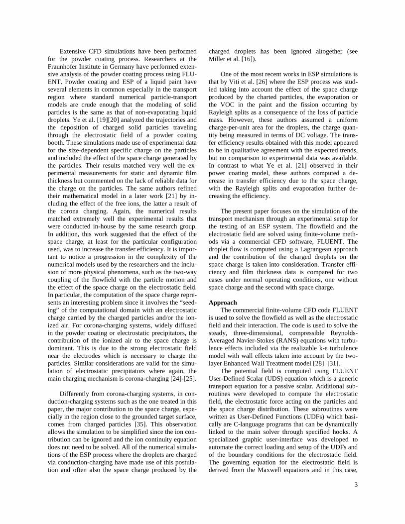
Figure 1. Flow diagram of the iterative procedure for the computation of the electrostatic field with and without space charge.

5

The trajectory of each particle is calculated by in-tegration of the equation of motion:

( )

( ) pD

p

dF

dt

ρ ρρ−

= − + +pp E

uu u g F

where up is the particle velocity, FD is the particle

drag coefficient, assumed to be a sphere, g is the accel-eration of gravity, ρp is the density of the paint, and FE is the electrostatic force, computed from:

q=EF E φ= −∇E

In the above equation for the electrostatic force we

are making the assumption that the Coulomb force is dominant over other electrostatic forces such as the image charge, the dielectrophoretic and the dipole-dipole effect [12].

1.5 m

1.5 m

1.5

m

1.0 m

18 c

m

15 c

m

1.0 m

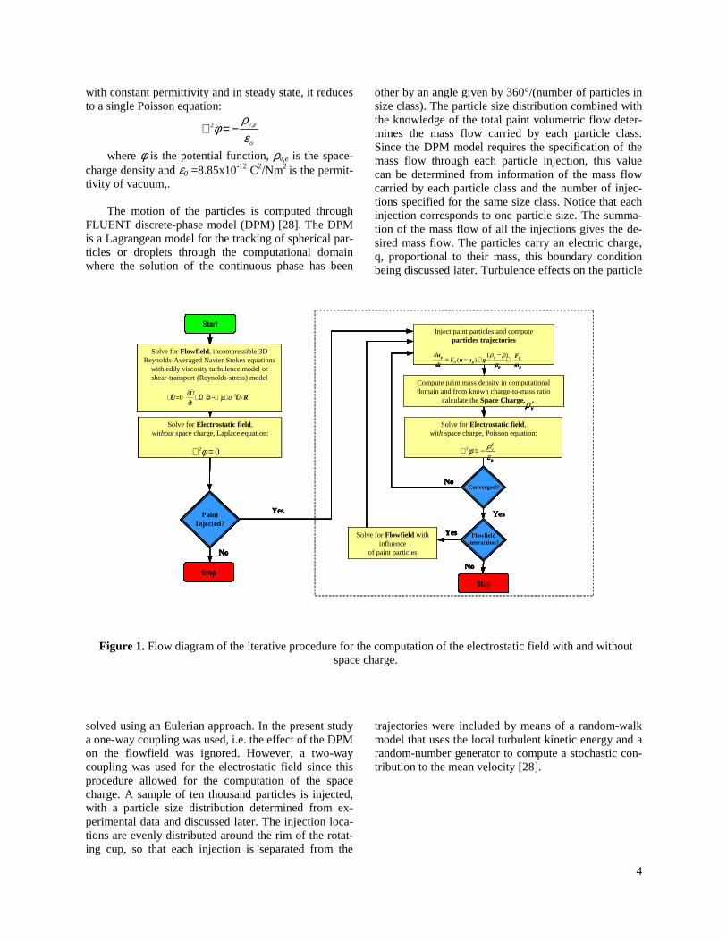
Figure 2 Computational domain lay-out and di-

mensions. The space charge, ρe, is computed through an itera-

tive process shown in the flow diagram of Figure 1. The flowfield and the electrostatic field without space charge (the latter governed by Lagrange equation) are computed using the appropriate boundary conditions. Once this solution is converged, the paint is injected using a sample file of 10000 particles with the correct particle size distribution and a specific charge. The ini-tial trajectories of this particle sample are computed according to the flowfield and the electrostatic field without space charge. The particles trajectories are used to “seed” the source term in the domain accordingly to the charge carried by each particle stream. This source

will vary over the computational domain and it deter-mines the space charge. That initial space charge is added as a source term to the Laplace equation for the electrostatic field so that we are now solving a Poisson equation. The equation is solved until convergence. When a new particle sample is injected and the process is repeated until overall convergence is reached. In or-der to make the setup of these simulations faster and more consistent a graphic-user interface was developed in the form of an add-on panel that is comparable to the standard FLUENT model panels.

Computational Domain and Grid The computational domain, shown in Figure 2, is a

rectangular box of size 1.5 meter a side which com-pletely encloses the paint gun and the target. The target is a flat plate 1m x 1m and 1 cm thick, its face placed at a distance of 200 mm. from the rim of the cup. For con-venience and to better control the grid density distribu-tion, the domain is decomposed into smaller connected volumes and an unstructured hexahedral mesh is used to discretize the entire domain.

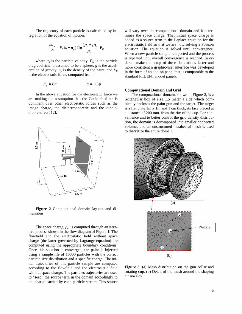
(a)

(b)

Figure 3. (a) Mesh distribution on the gun collar and rotating cup. (b) Detail of the mesh around the shaping air nozzles.

Nozzle

6

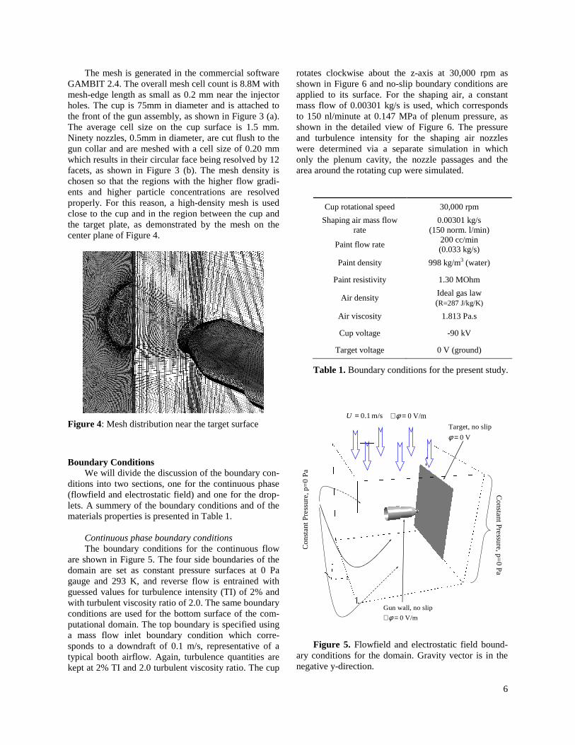
The mesh is generated in the commercial software GAMBIT 2.4. The overall mesh cell count is 8.8M with mesh-edge length as small as 0.2 mm near the injector holes. The cup is 75mm in diameter and is attached to the front of the gun assembly, as shown in Figure 3 (a). The average cell size on the cup surface is 1.5 mm. Ninety nozzles, 0.5mm in diameter, are cut flush to the gun collar and are meshed with a cell size of 0.20 mm which results in their circular face being resolved by 12 facets, as shown in Figure 3 (b). The mesh density is chosen so that the regions with the higher flow gradi-ents and higher particle concentrations are resolved properly. For this reason, a high-density mesh is used close to the cup and in the region between the cup and the target plate, as demonstrated by the mesh on the center plane of Figure 4.

Figure 4: Mesh distribution near the target surface

Boundary Conditions We will divide the discussion of the boundary con-

ditions into two sections, one for the continuous phase (flowfield and electrostatic field) and one for the drop-lets. A summery of the boundary conditions and of the materials properties is presented in Table 1.

Continuous phase boundary conditions The boundary conditions for the continuous flow

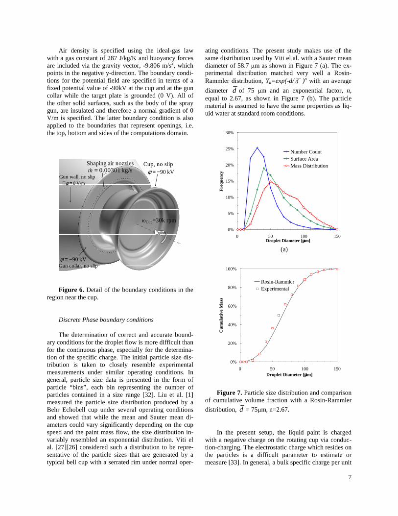
are shown in Figure 5. The four side boundaries of the domain are set as constant pressure surfaces at 0 Pa gauge and 293 K, and reverse flow is entrained with guessed values for turbulence intensity (TI) of 2% and with turbulent viscosity ratio of 2.0. The same boundary conditions are used for the bottom surface of the com-putational domain. The top boundary is specified using a mass flow inlet boundary condition which corre-sponds to a downdraft of 0.1 m/s, representative of a typical booth airflow. Again, turbulence quantities are kept at 2% TI and 2.0 turbulent viscosity ratio. The cup

rotates clockwise about the z-axis at 30,000 rpm as shown in Figure 6 and no-slip boundary conditions are applied to its surface. For the shaping air, a constant mass flow of 0.00301 kg/s is used, which corresponds to 150 nl/minute at 0.147 MPa of plenum pressure, as shown in the detailed view of Figure 6. The pressure and turbulence intensity for the shaping air nozzles were determined via a separate simulation in which only the plenum cavity, the nozzle passages and the area around the rotating cup were simulated.

Con

stan

t P

ress

ure,

p=

0 P

a

Co

nstan

t Pre

ssure

, p=0

Pa

0 V/mφ∇ =Target, no slip

0 Vφ =

0.1 m/sU =

Gun wall, no slip

0 V/mφ∇ =

Figure 5. Flowfield and electrostatic field bound-

ary conditions for the domain. Gravity vector is in the negative y-direction.

Cup rotational speed 30,000 rpm

Shaping air mass flow rate

0.00301 kg/s (150 norm. l/min)

Paint flow rate 200 cc/min (0.033 kg/s)

Paint density 998 kg/m3 (water)

Paint resistivity 1.30 MOhm

Air density Ideal gas law (R=287 J/kg/K)

Air viscosity 1.813 Pa.s

Cup voltage -90 kV

Target voltage 0 V (ground)

Table 1. Boundary conditions for the present study.

7

Air density is specified using the ideal-gas law with a gas constant of 287 J/kg/K and buoyancy forces are included via the gravity vector, -9.806 m/s2, which points in the negative y-direction. The boundary condi-tions for the potential field are specified in terms of a fixed potential value of -90kV at the cup and at the gun collar while the target plate is grounded (0 V). All of the other solid surfaces, such as the body of the spray gun, are insulated and therefore a normal gradient of 0 V/m is specified. The latter boundary condition is also applied to the boundaries that represent openings, i.e. the top, bottom and sides of the computations domain.

Figure 6. Detail of the boundary conditions in the

region near the cup. Discrete Phase boundary conditions The determination of correct and accurate bound-

ary conditions for the droplet flow is more difficult than for the continuous phase, especially for the determina-tion of the specific charge. The initial particle size dis-tribution is taken to closely resemble experimental measurements under similar operating conditions. In general, particle size data is presented in the form of particle “bins”, each bin representing the number of particles contained in a size range [32]. Liu et al. [1] measured the particle size distribution produced by a Behr Echobell cup under several operating conditions and showed that while the mean and Sauter mean di-ameters could vary significantly depending on the cup speed and the paint mass flow, the size distribution in-variably resembled an exponential distribution. Viti el al. [27][26] considered such a distribution to be repre-sentative of the particle sizes that are generated by a typical bell cup with a serrated rim under normal oper-

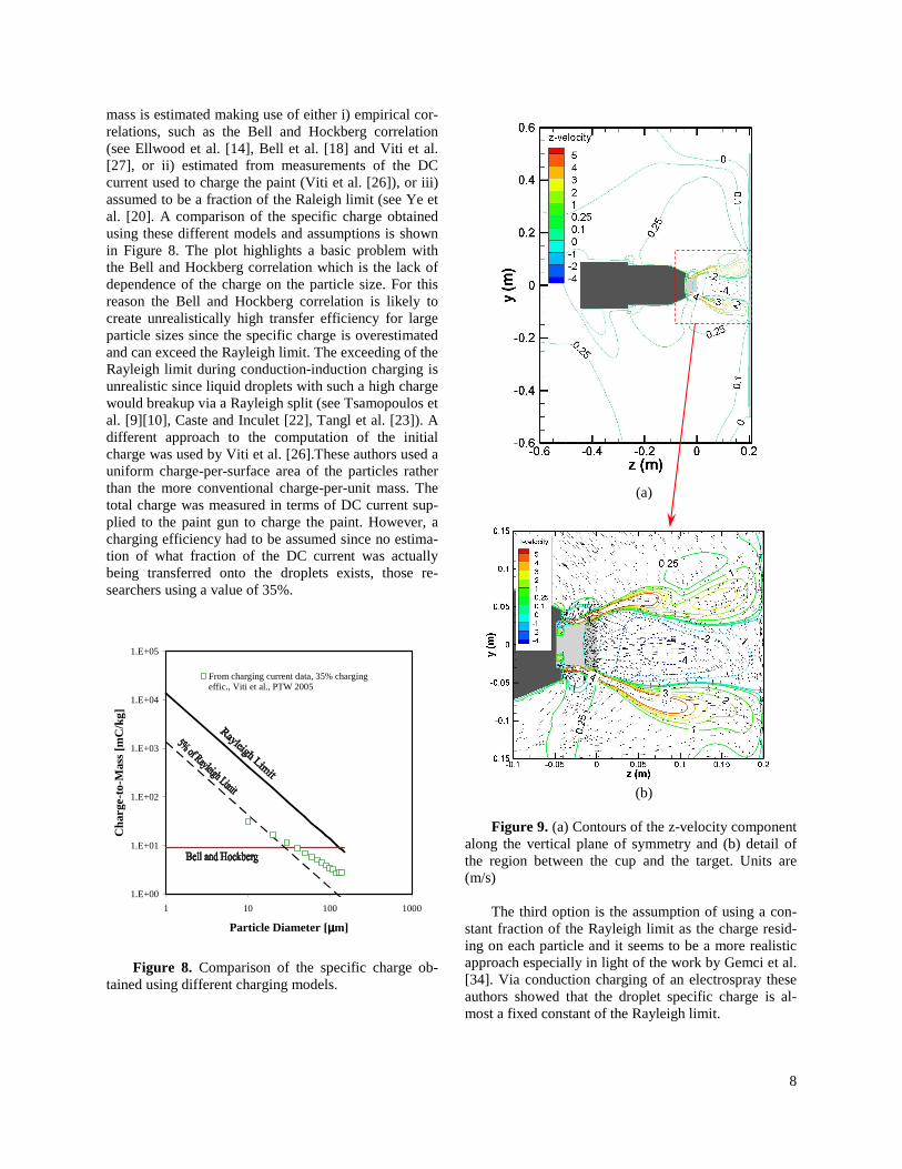
ating conditions. The present study makes use of the same distribution used by Viti el al. with a Sauter mean diameter of 58.7 µm as shown in Figure 7 (a). The ex-perimental distribution matched very well a Rosin-Rammler distribution, Yd=exp(-d/ d )n with an average

diameter d of 75 µm and an exponential factor, n, equal to 2.67, as shown in Figure 7 (b). The particle material is assumed to have the same properties as liq-uid water at standard room conditions.

0%

5%

10%

15%

20%

25%

30%

0 50 100 150Droplet Diameter [µµµµm]

Fre

quen

cy

Number CountSurface AreaMass Distribution

(a)

0%

20%

40%

60%

80%

100%

0 50 100 150Droplet Diameter [µµµµm]

Cum

ulat

ive

Mas

s

Rosin-RammlerExperimental

Figure 7. Particle size distribution and comparison

of cumulative volume fraction with a Rosin-Rammler

distribution, d = 75µm, n=2.67. In the present setup, the liquid paint is charged

with a negative charge on the rotating cup via conduc-tion-charging. The electrostatic charge which resides on the particles is a difficult parameter to estimate or measure [33]. In general, a bulk specific charge per unit

ωCup=30k rpm

Cup, no slipShaping air nozzles

90 kVφ = −0.00301 kg/sm =&

Gun collar, no slip90 kVφ = −

Gun wall, no slip0 V/mφ∇ =

8

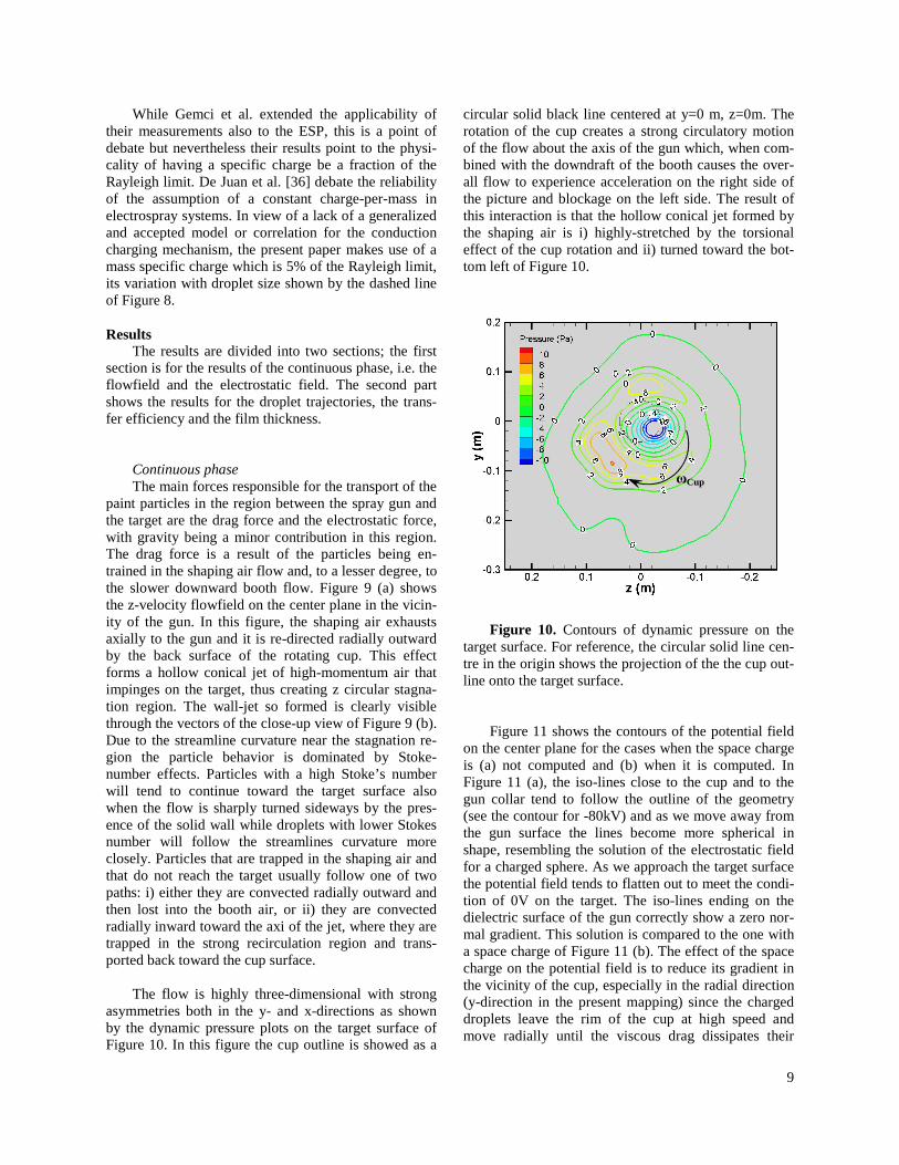
mass is estimated making use of either i) empirical cor-relations, such as the Bell and Hockberg correlation (see Ellwood et al. [14], Bell et al. [18] and Viti et al. [27], or ii) estimated from measurements of the DC current used to charge the paint (Viti et al. [26]), or iii) assumed to be a fraction of the Raleigh limit (see Ye et al. [20]. A comparison of the specific charge obtained using these different models and assumptions is shown in Figure 8. The plot highlights a basic problem with the Bell and Hockberg correlation which is the lack of dependence of the charge on the particle size. For this reason the Bell and Hockberg correlation is likely to create unrealistically high transfer efficiency for large particle sizes since the specific charge is overestimated and can exceed the Rayleigh limit. The exceeding of the Rayleigh limit during conduction-induction charging is unrealistic since liquid droplets with such a high charge would breakup via a Rayleigh split (see Tsamopoulos et al. [9][10], Caste and Inculet [22], Tangl et al. [23]). A different approach to the computation of the initial charge was used by Viti et al. [26].These authors used a uniform charge-per-surface area of the particles rather than the more conventional charge-per-unit mass. The total charge was measured in terms of DC current sup-plied to the paint gun to charge the paint. However, a charging efficiency had to be assumed since no estima-tion of what fraction of the DC current was actually being transferred onto the droplets exists, those re-searchers using a value of 35%.

1.E+00

1.E+01

1.E+02

1.E+03

1.E+04

1.E+05

1 10 100 1000

Particle Diameter [µµµµm]

Cha

rge-

to-M

ass

[mC

/kg]

From charging current data, 35% chargingeffic., Viti et al., PTW 2005

Figure 8. Comparison of the specific charge ob-tained using different charging models.

(a)

(b)

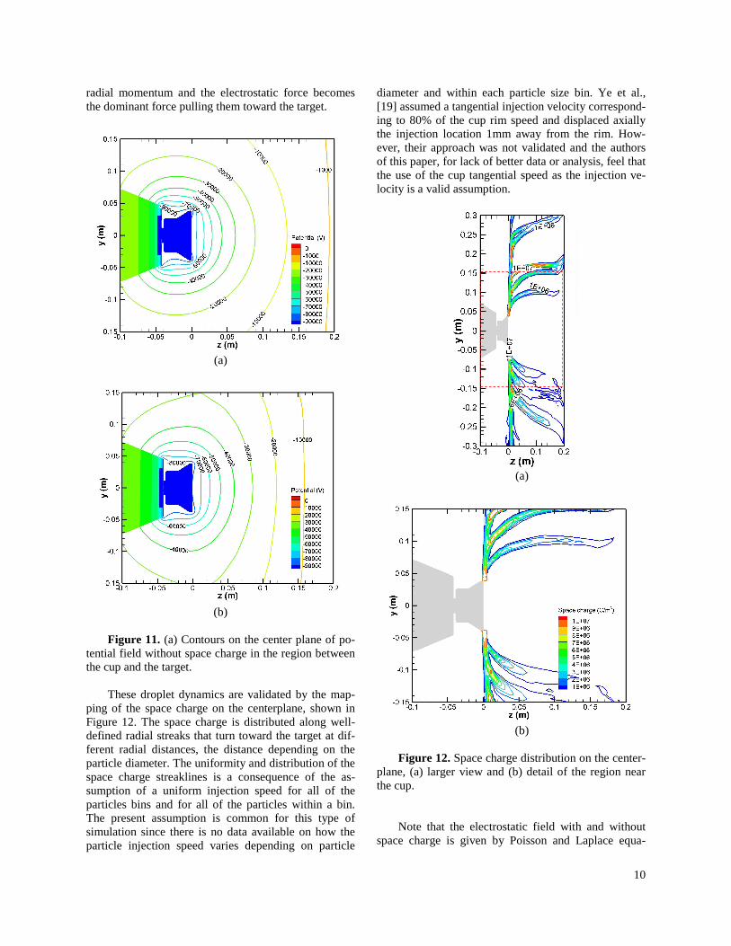
Figure 9. (a) Contours of the z-velocity component

along the vertical plane of symmetry and (b) detail of the region between the cup and the target. Units are (m/s)

The third option is the assumption of using a con-

stant fraction of the Rayleigh limit as the charge resid-ing on each particle and it seems to be a more realistic approach especially in light of the work by Gemci et al. [34]. Via conduction charging of an electrospray these authors showed that the droplet specific charge is al-most a fixed constant of the Rayleigh limit.

9

While Gemci et al. extended the applicability of their measurements also to the ESP, this is a point of debate but nevertheless their results point to the physi-cality of having a specific charge be a fraction of the Rayleigh limit. De Juan et al. [36] debate the reliability of the assumption of a constant charge-per-mass in electrospray systems. In view of a lack of a generalized and accepted model or correlation for the conduction charging mechanism, the present paper makes use of a mass specific charge which is 5% of the Rayleigh limit, its variation with droplet size shown by the dashed line of Figure 8.

Results

The results are divided into two sections; the first section is for the results of the continuous phase, i.e. the flowfield and the electrostatic field. The second part shows the results for the droplet trajectories, the trans-fer efficiency and the film thickness.

Continuous phase The main forces responsible for the transport of the

paint particles in the region between the spray gun and the target are the drag force and the electrostatic force, with gravity being a minor contribution in this region. The drag force is a result of the particles being en-trained in the shaping air flow and, to a lesser degree, to the slower downward booth flow. Figure 9 (a) shows the z-velocity flowfield on the center plane in the vicin-ity of the gun. In this figure, the shaping air exhausts axially to the gun and it is re-directed radially outward by the back surface of the rotating cup. This effect forms a hollow conical jet of high-momentum air that impinges on the target, thus creating z circular stagna-tion region. The wall-jet so formed is clearly visible through the vectors of the close-up view of Figure 9 (b). Due to the streamline curvature near the stagnation re-gion the particle behavior is dominated by Stoke-number effects. Particles with a high Stoke’s number will tend to continue toward the target surface also when the flow is sharply turned sideways by the pres-ence of the solid wall while droplets with lower Stokes number will follow the streamlines curvature more closely. Particles that are trapped in the shaping air and that do not reach the target usually follow one of two paths: i) either they are convected radially outward and then lost into the booth air, or ii) they are convected radially inward toward the axi of the jet, where they are trapped in the strong recirculation region and trans-ported back toward the cup surface.

The flow is highly three-dimensional with strong

asymmetries both in the y- and x-directions as shown by the dynamic pressure plots on the target surface of Figure 10. In this figure the cup outline is showed as a

circular solid black line centered at y=0 m, z=0m. The rotation of the cup creates a strong circulatory motion of the flow about the axis of the gun which, when com-bined with the downdraft of the booth causes the over-all flow to experience acceleration on the right side of the picture and blockage on the left side. The result of this interaction is that the hollow conical jet formed by the shaping air is i) highly-stretched by the torsional effect of the cup rotation and ii) turned toward the bot-tom left of Figure 10.

Figure 10. Contours of dynamic pressure on the

target surface. For reference, the circular solid line cen-tre in the origin shows the projection of the the cup out-line onto the target surface.

Figure 11 shows the contours of the potential field

on the center plane for the cases when the space charge is (a) not computed and (b) when it is computed. In Figure 11 (a), the iso-lines close to the cup and to the gun collar tend to follow the outline of the geometry (see the contour for -80kV) and as we move away from the gun surface the lines become more spherical in shape, resembling the solution of the electrostatic field for a charged sphere. As we approach the target surface the potential field tends to flatten out to meet the condi-tion of 0V on the target. The iso-lines ending on the dielectric surface of the gun correctly show a zero nor-mal gradient. This solution is compared to the one with a space charge of Figure 11 (b). The effect of the space charge on the potential field is to reduce its gradient in the vicinity of the cup, especially in the radial direction (y-direction in the present mapping) since the charged droplets leave the rim of the cup at high speed and move radially until the viscous drag dissipates their

ωCup

10

radial momentum and the electrostatic force becomes the dominant force pulling them toward the target.

(a)

(b)

Figure 11. (a) Contours on the center plane of po-

tential field without space charge in the region between the cup and the target.

These droplet dynamics are validated by the map-

ping of the space charge on the centerplane, shown in Figure 12. The space charge is distributed along well-defined radial streaks that turn toward the target at dif-ferent radial distances, the distance depending on the particle diameter. The uniformity and distribution of the space charge streaklines is a consequence of the as-sumption of a uniform injection speed for all of the particles bins and for all of the particles within a bin. The present assumption is common for this type of simulation since there is no data available on how the particle injection speed varies depending on particle

diameter and within each particle size bin. Ye et al., [19] assumed a tangential injection velocity correspond-ing to 80% of the cup rim speed and displaced axially the injection location 1mm away from the rim. How-ever, their approach was not validated and the authors of this paper, for lack of better data or analysis, feel that the use of the cup tangential speed as the injection ve-locity is a valid assumption.

(a)

(b)

Figure 12. Space charge distribution on the center-

plane, (a) larger view and (b) detail of the region near the cup.

Note that the electrostatic field with and without

space charge is given by Poisson and Laplace equa-

11

tions, respectively. Both of these differential equations are linear and for simple geometries can be solved in closed form. However, the coupling with the flowfield and, to a lesser degree, the complex geometry makes the solution of the electrostatic field a non-trivial task which needs the use of an iterative procedure.

-1.E+05

-9.E+04

-8.E+04

-7.E+04

-6.E+04

-5.E+04

-4.E+04

-3.E+04

-2.E+04

-1.E+04

0.E+00

-0.01 0.04 0.09 0.14 0.19

z-distance (m)

Pot

enti

al (

V)

0.E+00

3.E+05

6.E+05

9.E+05

1.E+06

Electrostatic F

ield (V/m

)

No space charge

With space charge

E-field

Potential

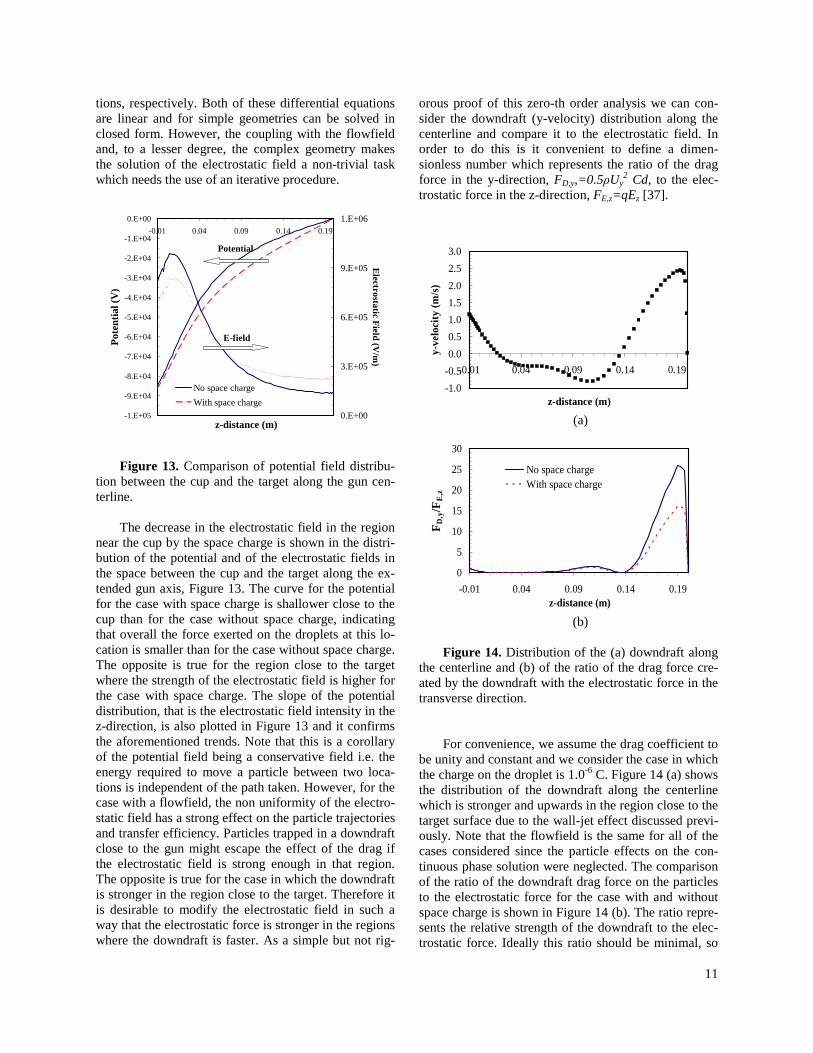
Figure 13. Comparison of potential field distribu-tion between the cup and the target along the gun cen-terline.

The decrease in the electrostatic field in the region

near the cup by the space charge is shown in the distri-bution of the potential and of the electrostatic fields in the space between the cup and the target along the ex-tended gun axis, Figure 13. The curve for the potential for the case with space charge is shallower close to the cup than for the case without space charge, indicating that overall the force exerted on the droplets at this lo-cation is smaller than for the case without space charge. The opposite is true for the region close to the target where the strength of the electrostatic field is higher for the case with space charge. The slope of the potential distribution, that is the electrostatic field intensity in the z-direction, is also plotted in Figure 13 and it confirms the aforementioned trends. Note that this is a corollary of the potential field being a conservative field i.e. the energy required to move a particle between two loca-tions is independent of the path taken. However, for the case with a flowfield, the non uniformity of the electro-static field has a strong effect on the particle trajectories and transfer efficiency. Particles trapped in a downdraft close to the gun might escape the effect of the drag if the electrostatic field is strong enough in that region. The opposite is true for the case in which the downdraft is stronger in the region close to the target. Therefore it is desirable to modify the electrostatic field in such a way that the electrostatic force is stronger in the regions where the downdraft is faster. As a simple but not rig-

orous proof of this zero-th order analysis we can con-sider the downdraft (y-velocity) distribution along the centerline and compare it to the electrostatic field. In order to do this is it convenient to define a dimen-sionless number which represents the ratio of the drag force in the y-direction, FD,y,=0.5ρUy

2 Cd, to the elec-trostatic force in the z-direction, FE,z=qEz [37].

-1.0

-0.5

0.0

0.5

1.0

1.5

2.0

2.5

3.0

-0.01 0.04 0.09 0.14 0.19

z-distance (m)

y-ve

loci

ty (

m/s

)

(a)

0

5

10

15

20

25

30

-0.01 0.04 0.09 0.14 0.19z-distance (m)

FD

,y/F

E,z

No space chargeWith space charge

(b)

Figure 14. Distribution of the (a) downdraft along

the centerline and (b) of the ratio of the drag force cre-ated by the downdraft with the electrostatic force in the transverse direction.

For convenience, we assume the drag coefficient to

be unity and constant and we consider the case in which the charge on the droplet is 1.0-6 C. Figure 14 (a) shows the distribution of the downdraft along the centerline which is stronger and upwards in the region close to the target surface due to the wall-jet effect discussed previ-ously. Note that the flowfield is the same for all of the cases considered since the particle effects on the con-tinuous phase solution were neglected. The comparison of the ratio of the downdraft drag force on the particles to the electrostatic force for the case with and without space charge is shown in Figure 14 (b). The ratio repre-sents the relative strength of the downdraft to the elec-trostatic force. Ideally this ratio should be minimal, so

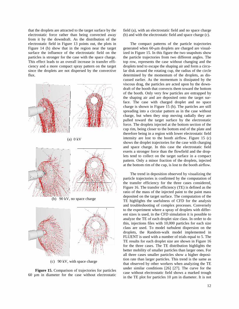
12

that the droplets are attracted to the target surface by the electrostatic force rather than being convected away from it by the downdraft. As the distribution of the electrostatic field in Figure 13 points out, the plots in Figure 14 (b) show that in the region near the target surface the influence of the electrostatic field on the particles is stronger for the case with the space charge. This effect leads to an overall increase in transfer effi-ciency and a more compact spray pattern on the target since the droplets are not dispersed by the convective flux.

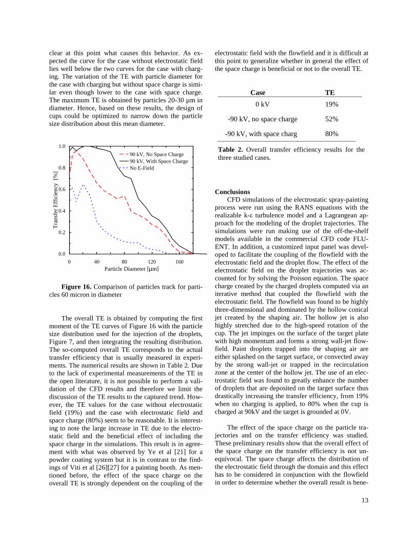
(a) 0 kV

(b) 90 kV, no space charge

(c) 90 kV, with space charge Figure 15. Comparison of trajectories for particles

60 µm in diameter for the case without electrostatic

field (a), with an electrostatic field and no space charge (b) and with the electrostatic field and space charge (c).

The compact patterns of the particle trajectories

generated when 60-µm droplets are charged are visual-ized in Figure 15. In this figure the two snapshots show the particle trajectories from two different angles. The top row, represents the case without changing and the droplets tend to escape the shaping air and form a circu-lar disk around the rotating cup, the radius of the circle determined by the momentum of the droplets, as dis-cussed earlier. As the momentum is dissipated by the viscous drag, the particles are acted upon by the down-draft of the booth that convects them toward the bottom of the booth. Only very few particles are entrapped by the shaping air and are deposited onto the target sur-face. The case with charged droplet and no space charge is shown in Figure 15 (b). The particles are still spreading into a circular pattern as in the case without charge, but when they stop moving radially they are pulled toward the target surface by the electrostatic force. The droplets injected at the bottom section of the cup rim, being closer to the bottom end of the plate and therefore being in a region with lower electrostatic field intensity are lost to the booth airflow. Figure 15 (c) shows the droplet trajectories for the case with charging and space charge. In this case the electrostatic field exerts a stronger force than the flowfield and the drop-lets tend to collect on the target surface in a compact pattern. Only a minor fraction of the droplets, injected at the bottom rim of the cup, is lost to the booth airflow.

The trend in deposition observed by visualizing the

particle trajectories is confirmed by the computation of the transfer efficiency for the three cases considered, Figure 16. The transfer efficiency (TE) is defined as the ratio of the mass of the injected paint to the paint mass deposited on the target surface. The computation of the TE highlights the usefulness of CFD for the analysis and troubleshooting of complex processes. Conversely to the experiment where a spray of droplets with differ-ent sizes is used, in the CFD simulation it is possible to analyze the TE of each droplet size class. In order to do this, injections files with 10,000 particles for each size class are used. To model turbulent dispersion on the droplets, the Random-walk model implemented in FLUENT is used with a number of trials equal to 5. The TE results for each droplet size are shown in Figure 16 for the three cases. The TE distribution highlights the better mobility of smaller particles than larger ones. For all three cases smaller particles show a higher deposi-tion rate than larger particles. This trend is the same as that observed by other workers when analyzing the TE under similar conditions [26] [27]. The curve for the case without electrostatic field shows a marked trough in the TE plot for particles 10 µm in diameter. It is not

13

clear at this point what causes this behavior. As ex-pected the curve for the case without electrostatic field lies well below the two curves for the case with charg-ing. The variation of the TE with particle diameter for the case with charging but without space charge is simi-lar even though lower to the case with space charge. The maximum TE is obtained by particles 20-30 µm in diameter. Hence, based on these results, the design of cups could be optimized to narrow down the particle size distribution about this mean diameter.

0.0

0.2

0.4

0.6

0.8

1.0

0 40 80 120 160Particle Diameter [µm]

Tra

nsf

er

Effi

cie

ncy

[%

]

90 kV, No Space Charge90 kV, With Space ChargeNo E-Field

Figure 16. Comparison of particles track for parti-

cles 60 micron in diameter The overall TE is obtained by computing the first

moment of the TE curves of Figure 16 with the particle size distribution used for the injection of the droplets, Figure 7, and then integrating the resulting distribution. The so-computed overall TE corresponds to the actual transfer efficiency that is usually measured in experi-ments. The numerical results are shown in Table 2. Due to the lack of experimental measurements of the TE in the open literature, it is not possible to perform a vali-dation of the CFD results and therefore we limit the discussion of the TE results to the captured trend. How-ever, the TE values for the case without electrostatic field (19%) and the case with electrostatic field and space charge (80%) seem to be reasonable. It is interest-ing to note the large increase in TE due to the electro-static field and the beneficial effect of including the space charge in the simulations. This result is in agree-ment with what was observed by Ye et al [21] for a powder coating system but it is in contrast to the find-ings of Viti et al [26][27] for a painting booth. As men-tioned before, the effect of the space charge on the overall TE is strongly dependent on the coupling of the

electrostatic field with the flowfield and it is difficult at this point to generalize whether in general the effect of the space charge is beneficial or not to the overall TE.

Conclusions CFD simulations of the electrostatic spray-painting

process were run using the RANS equations with the realizable k-ε turbulence model and a Lagrangean ap-proach for the modeling of the droplet trajectories. The simulations were run making use of the off-the-shelf models available in the commercial CFD code FLU-ENT. In addition, a customized input panel was devel-oped to facilitate the coupling of the flowfield with the electrostatic field and the droplet flow. The effect of the electrostatic field on the droplet trajectories was ac-counted for by solving the Poisson equation. The space charge created by the charged droplets computed via an iterative method that coupled the flowfield with the electrostatic field. The flowfield was found to be highly three-dimensional and dominated by the hollow conical jet created by the shaping air. The hollow jet is also highly stretched due to the high-speed rotation of the cup. The jet impinges on the surface of the target plate with high momentum and forms a strong wall-jet flow-field. Paint droplets trapped into the shaping air are either splashed on the target surface, or convected away by the strong wall-jet or trapped in the recirculation zone at the center of the hollow jet. The use of an elec-trostatic field was found to greatly enhance the number of droplets that are deposited on the target surface thus drastically increasing the transfer efficiency, from 19% when no charging is applied, to 80% when the cup is charged at 90kV and the target is grounded at 0V.

The effect of the space charge on the particle tra-

jectories and on the transfer efficiency was studied. These preliminary results show that the overall effect of the space charge on the transfer efficiency is not un-equivocal. The space charge affects the distribution of the electrostatic field through the domain and this effect has to be considered in conjunction with the flowfield in order to determine whether the overall result is bene-

Case TE

0 kV 19%

-90 kV, no space charge 52%

-90 kV, with space charge 80%

Table 2. Overall transfer efficiency results for the three studied cases.

14

ficial or not to the transfer efficiency. A dimensionless number, the ratio of the downdraft aerodynamic force to the electrostatic force is proposed as a tool to better understand and characterize the interaction of the flow-field with the electrostatic field via the particle flow.

CFD techniques were found to be able to ade-

quately resolve the complex flowfield and electrostatic field as well as the paint droplet trajectories. The nu-merical approach proved to be useful in providing valu-able information for the optimization of coating sys-tems.

Acknowledgments The authors would like to thank Satya Kondle for

his assistance in producing the results used in this pa-per.

References 1. Liu, Y., Lai, M., Im, K., Sankagiri, N., Loch, T. And

Nivi, H., An experimental investigation of spray transfer processes in an electrostatic rotating bell applicator, SAE Paper 982290, 1998.

2. Bailey, A., The science and technology of electro-static powder spraying, transport and coating, Jour-nal of Electrostatics 45, 85-120, 1998.

3. Lefebvre, A., Atomization and sprays, Hemisphere Publishing Company, 1989.

4. Sirignano, W.A., Fluid dynamics and transport of droplets and sprays, Cambridge University Press, 1999.

5. Lin, S.P., Breakup of liquid sheets and jets, Cam-bridge University Press, 2003.

6. Lin, S.P., Reitz, R.D., “Drop and spray formation from liquid jet”, Annual Review of Fluid Mechan-ics, Vol. 30, pp. 85-105, 1998.

7. Reitz, D., Bracco, F. V., “Mechanism of Atomiza-tion of a Liquid Jet”, Physics of Fluids, 26 (10) (1982).

8. Frohn, A., Roth, N., Dynamics of Droplets, 1st Ed. Springer-Verlag, New York, 2000.

9. Tsamopoulos, J.A., Akylas, T. R., Browns, R.A., Dynamics of charged drop break-ups, Proc. of the Royal Society, London, 1985, Vol. 401, pp. 67-88.

10. Tsamopoulos, J.A., Nonlinear Dynamics and break-up of charged drops, American Institute of Physics, Conference proceedings Series, No. 197, pp. 169-187, 1989.

11. Kazama, S., Japan Society of Automotive Engi-neers, Review 24, pp. 489-494, 2003.

12. Li, A. and Ahmadi, G., Aerosol particle deposition with electrostatic attraction in a turbulent channel

flow, Journal of Colloid Interface Sciences, Vol. 158, 476-482, 1993.

13. Hackberg, B., Lundqvist, S., Carlsson, B., Hog-berg, T., A theoretical model for electrostatic spraying and coating, Journal of Electrostatics, Vol. 14, 1983, pp.255-268.

14. Ellwood, K.R.J., Braslaw, J., A finite-element model for an electrostatic bell sprayer, Journal of Electrostatic, Vol. 23, 1998, pp. 1-23.

15. Bottner, C.-U. , Sommerfeld, M., Euler/Lagrange calculations of particle motion in turbulent flow coupled with an electric field, European Congress on Computational Methods in Applied Sciences and Engineering, CFD Conference, Swansea, UK, 4-7 September 2001.

16. Miller, R., Strumolo, G., Babu, V., Braslaw, J., Mehta, M., Transient CFD simulations of a bell sprayer, Proc. of the Intl. Body Engineering Con-ference and Exposition, Detroit, Michigan, Sep-tember 1998, SAE Paper 982291.

17. Su-Im, K., Yu, J. S.-T., Ming, C.-L., Meredith, W., Simulation of the shaping air and spray transport in electrostatic rotary bell painting process, Proc. of the Intl. Body Engineering Conference and Exhibi-tion, Paris, France, July 2002, SAE Paper 2002-01-2106.

18. Bell, G. C, Hochberg, J., Mechanics electrostatic atomization, transport, and deposition of coatings, in G. D. Parfitt (Ed.), Organic Coatings Science and Technology, Vol. 5, Marcel-Dekker, New York, pp. 325-357, 1981.

19. Ye, Q. , Steigleder, T., Scheibe, A., J. Dominick, J., Numerical simulation of the electrostatic pow-der coating process with a corona spraygun, Jour-nal of Electrostatics, Vol. 54, pp 189-205, 2002.

20. Ye, Q., Dominick, J., Scheibe, A., Numerical simu-lation of spray painting in the automotive industry, 1st European Automotive CFD Conference, Bin-gen, Germany, June 2003

21. Ye, Q., Dominick, J., On the simulation of space charge in electrostatic powder coating with a co-rona spray gun, Powder Technology Vol. 135– 136, pp. 250– 260, 2003.

22. Castle, G.S.P., Inculet, I.I., Induction charge limit of small water droplets, Institute of Physics Con-ference Series 118, Session 3, presented at electro-statics ’91, Oxford, 1991.

23. Tang1, K., Smith, R.D., Theoretical prediction of charged droplet evaporation and fission in elec-trospray ionization, International Journal of Mass Spectrometry Vol. 185/186/187, pp.97-105, 1999.

24. Zamankhan, P., Ahmadi, G., Coupling effects of the flow and electric fields in electrostatic precipi-tators, Journal of Applied Physics, Volume 96, No. 12, 2004.

15

25. Medlin, Andrew J., Electrohydrodynamic Model-ling of Fine Particle Collection in Electrostatic Pre-cipitators, Ph.D. Dissertation, University of New South Wales, Australia, May 1998.

26. Viti, V., Salazar, A., Saito, S., Numerical Investi-gation of the Evaporation and Break-up of Charged Droplets in an Automotive Paint Booth, Paint Technology Workshop, Lexington, KY, USA, 12-13 October 2005.

27. Viti, V., Salazar, A., Saito, S., A Numerical Study of the Coupling between the Flowfield and the Electrostatic Field inside an Automotive Spray Paint Booth, Transactions of the IASME, Vol. , 2005.

28. Fluent, Inc., “Fluent 6.3 User Guide”, Lebanon, NH, USA, 2006.

29. Kader., B., Temperature and Concentration Profiles in Fully Turbulent Boundary Layers, International Journal of Heat and Mass Transfer, Vol. 24, No. 9, pp.1541-1544, 1981.

30. Wolfstein., M., The Velocity and Temperature Dis-tribution of One-Dimensional Flow with Turbu-lence Augmentation and Pressure Gradient, Inter-national Journal of Heat and Mass Transfer, Vol. 12, pp. 301-318, 1969.

31. Chen, H. C., Patel., V. C., Near-Wall Turbulence Models for Complex Flows Including Separation, AIAA Journal, Vol. 26, No. 6, pp. 641-648, 1988.

32. Hinds, W. C., “Aerosol Technology”, 2nd Ed., John Wiley and Sons, New York, ISBN 0-471-19410-7, 1999.

33. Zhao, S., Peter Castle, G.S., Adamiak, Z., Com-parison of conduction and induction charging in liquid spraying, Journal of Electrostatics Vol. 63 pp. 871-876, 2005.

34. Gemci, T., Hitron, R. Chigier, N., Measuring Charge-To-Mass Ratio Of Individual Droplets Us-ing Phase Doppler Interferometery, ILASS Ameri-cas, 15th Annual Conference on Liquid Atomiza-tion and Spray Systems, Madison, WI, May 2002

35. McCarthy, J. E., Senser, D.W., Specific charge measurements in electrostatic air sprays, Particu-late Science and Technology, Vol. 23, pp. 21-32, 2005.

36. De Juan, L., De La Mora, F., Charge and Size Dis-tributions of Electrospray Drops, Journal of Col-loids and Interface Science, Vol. 186, pp. 280-293, 1997.

37. Viti, V., Kitagawa, K., Internal communications, University of Kentucky/Aichi Institute of Technol-ogy, February-March 2006.

16

Documents

CFD Analysis of the Electrostatic Spray Painting Process ... M2-B-3.pdf · ILASS Americas, 21 st Annual Conference on Liquid Atomization and Spray Systems, Orlando, Florida, USA,