Embed Size (px)
Citation preview
SANDIA REPORT SAND2008-1688 Unlimited Release Printed April 2008
CFD Analysis of Rotating Two-Bladed Flatback Wind Turbine Rotor
David D. Chao and C.P. “Case” van Dam
Prepared by Sandia National Laboratories Albuquerque, New Mexico 87185 and Livermore, California 94550 Sandia is a multiprogram laboratory operated by Sandia Corporation, a Lockheed Martin Company, for the United States Department of Energy’s National Nuclear Security Administration under Contract DE-AC04-94AL85000. Approved for public release; further dissemination unlimited.

Issued by Sandia National Laboratories, operated for the United States Department of Energy by Sandia Corporation. NOTICE: This report was prepared as an account of work sponsored by an agency of the United States Government. Neither the United States Government, nor any agency thereof, nor any of their employees, nor any of their contractors, subcontractors, or their employees, make any warranty, express or implied, or assume any legal liability or responsibility for the accuracy, completeness, or usefulness of any information, apparatus, product, or process disclosed, or represent that its use would not infringe privately owned rights. Reference herein to any specific commercial product, process, or service by trade name, trademark, manufacturer, or otherwise, does not necessarily constitute or imply its endorsement, recommendation, or favoring by the United States Government, any agency thereof, or any of their contractors or subcontractors. The views and opinions expressed herein do not necessarily state or reflect those of the United States Government, any agency thereof, or any of their contractors. Printed in the United States of America. This report has been reproduced directly from the best available copy. Available to DOE and DOE contractors from U.S. Department of Energy Office of Scientific and Technical Information P.O. Box 62 Oak Ridge, TN 37831 Telephone: (865) 576-8401 Facsimile: (865) 576-5728 E-Mail: [email protected] Online ordering: http://www.osti.gov/bridge Available to the public from U.S. Department of Commerce National Technical Information Service 5285 Port Royal Rd. Springfield, VA 22161 Telephone: (800) 553-6847 Facsimile: (703) 605-6900 E-Mail: [email protected] Online order: http://www.ntis.gov/help/ordermethods.asp?loc=7-4-0#online
2
SAND2008-1688 Unlimited Release Printed April 2008
CFD Analysis of Rotating Two-Bladed Flatback Wind Turbine Rotor
David D. Chao and C. P. “Case” van Dam
Department of Mechanical and Aeronautical Engineering University of California One Shields Avenue
Davis, CA 95616-5294
Dale E. Berg, Sandia National Laboratories Technical Manager
Sandia Contract No. 15890
Abstract The effects of modifying the inboard portion of the NREL Phase VI rotor using a thickened, flatback version of the S809 design airfoil are studied using a three-dimensional Reynolds-averaged Navier-Stokes method. A motivation for using such a thicker airfoil design coupled with a blunt trailing edge is to alleviate structural constraints while reducing blade weight and maintaining the power performance of the rotor. The calculated results for the baseline Phase VI rotor are benchmarked against wind tunnel results obtained at 10, 7, and 5 meters per second. The calculated results for the modified rotor are compared against those of the baseline rotor. The results of this study demonstrate that a thick, flatback blade profile is viable as a bridge to connect structural requirements with aerodynamic performance in designing future wind turbine rotors.
3

Acknowledgements This project was supported by TPI Composites of Warren, Rhode Island under Contract 15890 – Revision 4 with Sandia National Laboratories. The primary members of the TPI team were Derek Berry (Principal Investigator) and Steve Nolet of TPI, Kevin Jackson of Dynamic Design, Michael Zuteck of MDZ Consulting and C.P. (Case) van Dam and his graduate students (David Chao for this particular effort) at the University of California at Davis. The members of the Sandia team were Tom Ashwill, Dale Berg (Technical Manager), Daniel Laird, Mark Rumsey, Herbert Sutherland, Paul Veers and Jose Zayas.
4

Table of Contents
Abstract.............................................................................................................................. 3
Acknowledgements ........................................................................................................... 4
Table of Contents .............................................................................................................. 5
List of Figures.................................................................................................................... 6
Introduction....................................................................................................................... 9
Flow Solver and Grid Generation ................................................................................. 10 Rotor Configurations .................................................................................................... 11 Grid Generation ............................................................................................................ 12
Results and Discussion.................................................................................................... 12 10 meters per second..................................................................................................... 13 7 meters per second....................................................................................................... 15 5 meters per second....................................................................................................... 16 Flow visualization......................................................................................................... 17 Some further analysis.................................................................................................... 18
Conclusions...................................................................................................................... 20
References........................................................................................................................ 77
5

List of Figures
Figure 1. Comparison of S809 design airfoil and modified S809 with 40% maximum thickness-to-chord ratio and 10% flatback trailing edge................................ 23
Figure 2. Tunnel views of geometric schedules for (a) baseline rotor blade, and (b) flatback rotor blade. ....................................................................................... 24
Figure 3. Views of computational grid for (a) baseline rotor, (b) flatback rotor, and (c) overall grid field. ............................................................................................ 25
Figure 4, Torque convergence histories for 10 m/s cases: (a) normal dynamic simulations, (b) dynamic simulations with 250% scaled velocities, and (c) source term with low-Mach preconditioning simulations.............................. 27
Figure 5. Comparison of spanwise normal force coefficients for baseline rotor at 10 m/s. ................................................................................................................. 29
Figure 6. Pressure coefficient distributions for baseline rotor at 10 m/s: (a) 30% span station, (b) 47% span station, (c) 63% span station, (d) 80% span station, and (e) 95% span station. ...................................................................................... 30
Figure 7. Comparison of spanwise normal force coefficients for flatback rotor at 10 m/s. ................................................................................................................. 33
Figure 8. Pressure coefficient distributions for flatback rotor at 10 m/s: (a) 30% span station, (b) 47% span station, (c) 63% span station, (d) 80% span station, and (e) 95% span station. ...................................................................................... 34
Figure 9. Smooth plots of velocity magnitude on suction side surface of rotor configurations at 10 m/s for (a) baseline rotor, and (b) flatback rotor. Black lines refer to span stations where Cp distributions are compared. Red line refers to 45% span station where blade geometries for both configurations become the same. Solutions obtained from source term with low-Mach preconditioning simulation............................................................................. 37
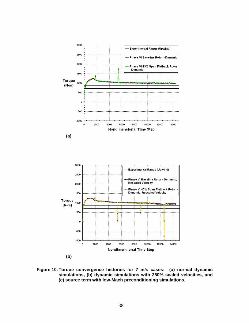
Figure 10. Torque convergence histories for 7 m/s cases: (a) normal dynamic simulations, (b) dynamic simulations with 250% scaled velocities, and (c) source term with low-Mach preconditioning simulations.............................. 38
Figure 11. Comparison of spanwise normal force coefficients for baseline rotor at 7 m/s......................................................................................................................... 40
6
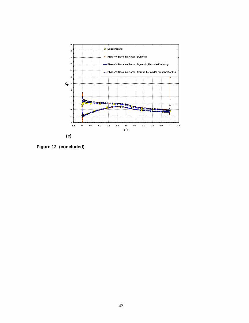
Figure 12. Pressure coefficient distributions for baseline rotor at 7 m/s: (a) 30% span station, (b) 47% span station, (c) 63% span station, (d) 80% span station, and (e) 95% span station. ...................................................................................... 41
Figure 13. Comparison of spanwise normal force coefficients for flatback rotor at 7 m/s......................................................................................................................... 44
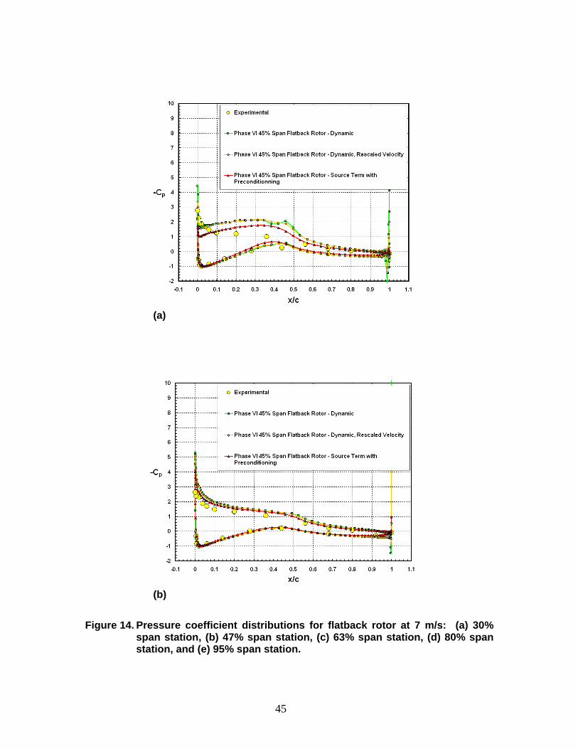
Figure 14. Pressure coefficient distributions for flatback rotor at 7 m/s: (a) 30% span station, (b) 47% span station, (c) 63% span station, (d) 80% span station, and (e) 95% span station. ...................................................................................... 45
Figure 15. Smooth plots of velocity magnitude on suction side surface of rotor configurations at 7 m/s for (a) baseline rotor, and (b) flatback rotor. Black lines refer to span stations where Cp distributions are compared. Red line refers to 45% span station where blade geometries for both configurations become the same. Solutions obtained from source term with low-Mach preconditioning simulation............................................................................. 48
Figure 16. Torque convergence histories for 5 m/s cases: (a) normal dynamic simulations, and (b) source term with low-Mach preconditioning simulations......................................................................................................................... 49
Figure 17. Comparison of spanwise normal force coefficients for baseline rotor at 5 m/s......................................................................................................................... 50
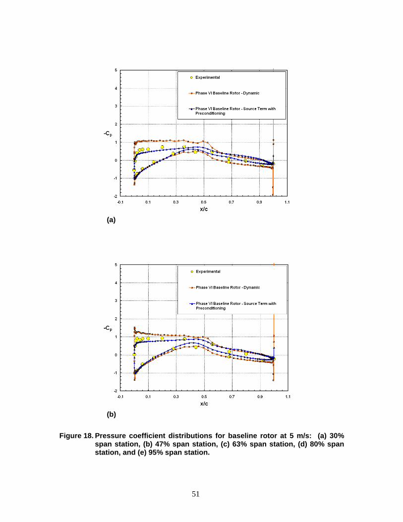
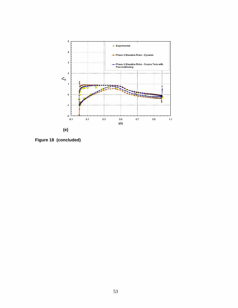
Figure 18. Pressure coefficient distributions for baseline rotor at 5 m/s: (a) 30% span station, (b) 47% span station, (c) 63% span station, (d) 80% span station, and (e) 95% span station. ...................................................................................... 51
Figure 19. Comparison of spanwise normal force coefficients for flatback rotor at 5 m/s......................................................................................................................... 54
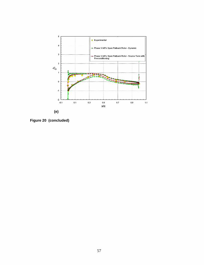
Figure 20. Pressure coefficient distributions for flatback rotor at 5 m/s: (a) 30% span station, (b) 47% span station, (c) 63% span station, (d) 80% span station, and (e) 95% span station. ...................................................................................... 55
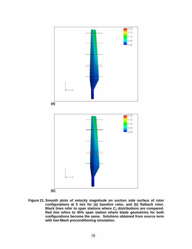
Figure 21. Smooth plots of velocity magnitude on suction side surface of rotor configurations at 5 m/s for (a) baseline rotor, and (b) flatback rotor. Black lines refer to span stations where Cp distributions are compared. Red line refers to 45% span station where blade geometries for both configurations become the same. Solutions obtained from source term with low-Mach preconditioning simulation............................................................................. 58
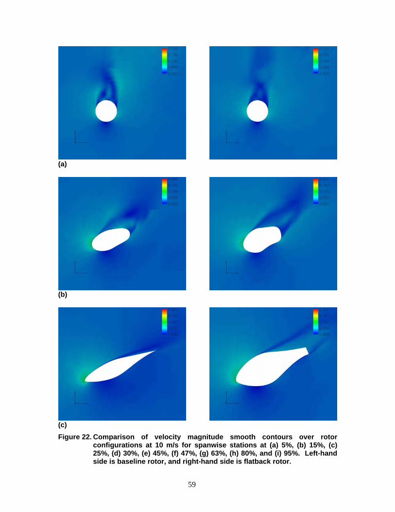
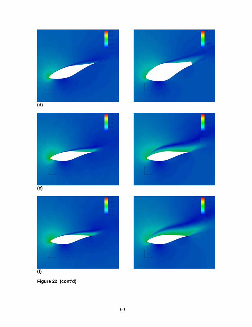
Figure 22. Comparison of velocity magnitude smooth contours over rotor configurations at 10 m/s for spanwise stations at (a) 5%, (b) 15%, (c) 25%, (d) 30%, (e) 45%, (f) 47%, (g) 63%, (h) 80%, and (i) 95%. Left-hand side is baseline rotor, and right-hand side is flatback rotor..................................................... 59
7
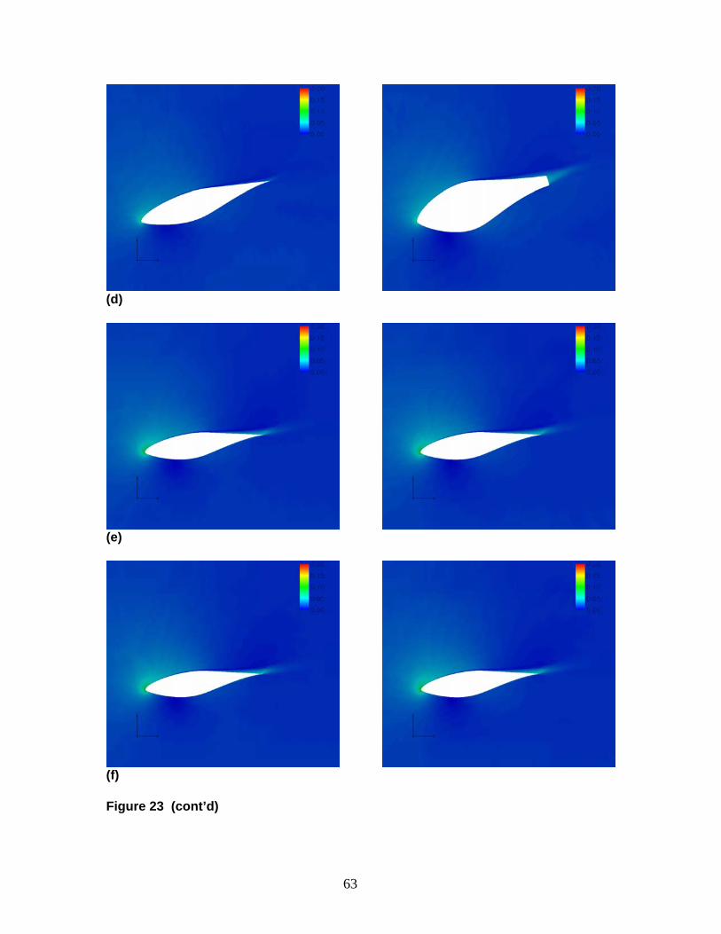
Figure 23. Comparison of velocity magnitude smooth contours over rotor configurations at 7 m/s for spanwise stations at (a) 5%, (b) 15%, (c) 25%, (d) 30%, (e) 45%, (f) 47%, (g) 63%, (h) 80%, and (i) 95%. Left-hand side is baseline rotor, and right-hand side is flatback rotor. .................................................................... 62
Figure 24. Comparison of velocity magnitude smooth contours over rotor configurations at 5 m/s for spanwise stations at (a) 5%, (b) 15%, (c) 25%, (d) 30%, (e) 45%, (f) 47%, (g) 63%, (h) 80%, and (i) 95%. Left-hand side is baseline rotor, and right-hand side is flatback rotor. .................................................................... 65
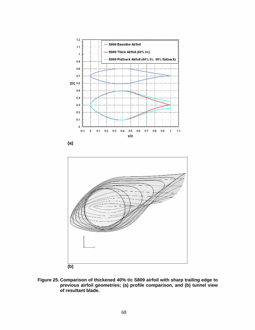
Figure 25. Comparison of thickened 40% t/c S809 airfoil with sharp trailing edge to previous airfoil geometries; (a) profile comparison, and (b) tunnel view of resultant blade. ............................................................................................... 68
Figure 26. Torque convergence histories of all three rotor configurations at (a) 7 m/s, and (b) 10 m/s. All solutions obtained using source term formulation with low-Mach preconditioning. ............................................................................ 69
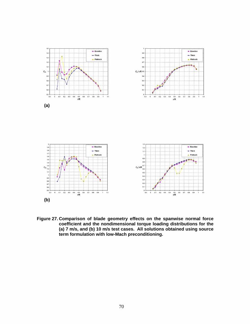
Figure 27. Comparison of blade geometry effects on the spanwise normal force coefficient and the nondimensional torque loading distributions for the (a) 7 m/s, and (b) 10 m/s test cases. All solutions obtained using source term formulation with low-Mach preconditioning. ................................................ 70
Figure 28. Comparison of blade geometry effects on pressure coefficient distributions at several spanwise stations for the 7 m/s test cases. All solutions obtained using source term formulation with low-Mach preconditioning.................... 71
Figure 29. Comparison of blade geometry effects on pressure coefficient distributions at several spanwise stations for the 10 m/s test cases. All solutions obtained using source term formulation with low-Mach preconditioning.................... 74
8
Introduction The primary goal of the Department of Energy (DOE) sponsored multi-phase Blade System Design Study (BSDS) has been for TPI Composites, Inc. to investigate and evaluate innovative design and manufacturing solutions for wind turbine blades in the one to ten megawatt size range. In this study, increasing the thickness of inboard blade section was identified as one of the key techniques for improving structural efficiency and reducing blade weight [1,2,3,4]. To improve the aerodynamic performance and structural efficiency of these thick airfoils, a series of blunt trailing edge airfoils was developed. These so-called flatback airfoils resulted in a blade design having excellent power performance characteristics, especially under soiled surface conditions. However, several items, identified in [4] and [5] required further investigation. First, very limited wind tunnel results that support field implementation of the flatback airfoil design are available in the open literature. Second, the flatback sections have excellent lift characteristics but high drag. Third, the flow about these section shapes is often unsteady as a result of bluff-body vortex shedding. Fourth, the effect of blade rotation on the flow along the blunt trailing edge and the performance characteristics of flatback section shapes require further study. This final item, a computational fluid dynamics (CFD) study of blade rotational effects on flow and performance characteristics of flatback airfoils, is addressed in this report. CFD codes based on the Reynolds-averaged Navier-Stokes equations are not yet practical tools to design and analyze wind turbines. As a result, CFD studies of rotating wind-turbine blades are still not very common. In part because of this lack of experience with these tools and the complexity of the flow problem, significant errors in rotor performance and blade aerodynamic load predictions are not uncommon [6]. This elevated risk of prediction error, in combination with the lack of experimental results for the rotor design presented in [4], led to the selection of the NREL Phase VI rotor [7,8] as the baseline configuration. Extensive wind-tunnel measurements are available for this rotor [7] and this allowed the validation of the computational tools applied in the current study before evaluating blade rotational effects on the performance characteristics of a modified rotor, including inboard flatback section shapes. In the following sections, the methods used to build the computational domain for two different rotor configurations and to generate the various solutions will be explained first. This will be followed by an analysis and discussion of the results obtained from computations at three different wind speeds. Finally, an overall conclusion will summarize the major findings from this study and suggest possible areas for further research and study.
9

Flow Solver and Grid Generation Computations were conducted with OVERFLOW, a three-dimensional compressible Reynolds-averaged Navier-Stokes flow solver developed by Buning et al. at NASA [9]. Steady and time-accurate solutions can be calculated on structured block or Chimera overset grids. OVERFLOW includes several turbulence models and incorporates various numerical schemes developed from previous research codes such as ARC2D [10] as well as other earlier flow solvers. Various zero-, one-, and two-equation turbulence models are available in OVERFLOW. However, since the objective of this study is not specifically a comparison of the different turbulence models but an evaluation of geometric effects on rotor performance, the Spalart-Allmaras model [11] was selected and used throughout the study. A main advantage of using OVERFLOW is it allows the rotor simulations to be conducted either as dynamic simulations with moving grid components or as pseudo-steady-state simulations with fixed grids through utilization of a source term formulation. In the source term implementation, instead of rotating the rotor grid itself, the rotational elements (Coriolis acceleration terms) are incorporated into the governing equations through use of a boundary condition which applies these terms to the surface boundary of the rotating grid components. This allows the resulting numerics to be solved in a manner similar to a steady-state algorithm. This utilization of a steady-state algorithm is significant because it allows the application of low-Mach preconditioning to the governing equations for improved convergence and solution quality at low Mach numbers [12]. For the highest wind speed used in this study at 10 m/s, the resulting Mach number is just less than 0.03. Including the angular rotation speed of 72 rpm, the effective freestream Mach number ranges from 0.03 near the rotor hub to still less than 0.12 at the tip. Low-Mach effects can be discernible for freestream Mach numbers as high as 0.25 [13]. In general, preconditioning is a technique used to remove stiffness from a system of equations. The RaNS equations are typically solved in an iterative fashion to achieve a steady-state solution. Although the steady-state solution is desired, the time-dependent equations are utilized to preserve the hyperbolic nature of the equations with respect to time for all Mach numbers. The system then has real eigenvalues and characteristic wave speeds such as aq + , where q is the total flow speed and a is the acoustic speed. This characteristic generally determines the maximum time step for a numerical algorithm. The rate of convergence to a solution is generally governed by q . This is the rate at which disturbances are propagated out of the computational domain [12]. For q << a (low-speed flows), stability requirements tend to force a time step so small that an inordinate amount of time steps is needed to achieve convergence, if convergence is achievable at all. Preconditioning seeks to rescale q to the same order of magnitude
10
as the acoustic speed so that convergence is achieved with a reduced number of time steps [12]. Although technically, preconditioning leads to a solution different from the non-preconditioned case, the preconditioned case should result in improved accuracy and convergence. The effects of low-Mach preconditioning will be detailed in the results section, but its integration into OVERFLOW simplifies the analysis of its effects. For the dynamic cases, the OVERFLOW solution is run in time-accurate mode with central differencing on the right-hand-side and ARC3D 3-factor block tridiagonal scheme on the left-hand-side for time stepping [9]. Second- and fourth-order dissipation values are kept at 0.0 and 0.04 for all cases. For the source term formulation with low-Mach preconditioning, the matrix dissipation scheme is used instead of the TLNS3D dissipation used for the dynamic simulations [9]. Matrix dissipation has been shown to provide better results with low-Mach preconditioning. In all cases, fully turbulent flow is assumed. Solutions are deemed converged when the torque has essentially flatlined. OVERFLOW also comes with the post processing FOMOCO toolset [14] comprising the two programs MIXSUR and OVERINT. This toolset calculates the lift, drag, and moment coefficients using surface integration. MIXSUR processes the original overset mesh configuration and forms body surface grids as specified by the user. Integration of the appropriate values is then performed using the OVERINT program to calculate all surface forces and moments. For the recent versions of OVERFLOW, MIXSUR is used first to create the body surfaces. OVERFLOW can then use the information to calculate the lift, drag, and moment coefficients at the end of each time step. Because the grid is set so that the center of rotation is the z-axis, the resulting yaw moment coefficient can be directly used to calculate the torque.
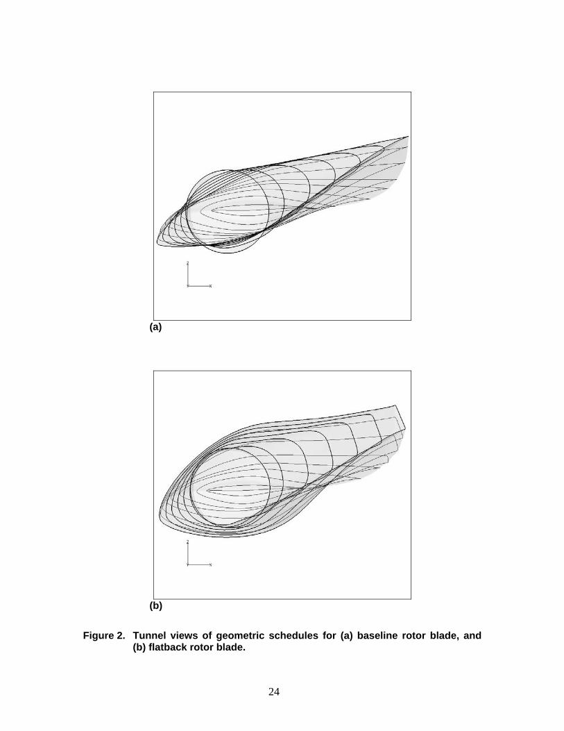
Rotor Configurations Two configurations are considered in this study. The first, referred to as the baseline rotor, is the original NREL Phase VI rotor utilizing the S809 airfoil with a 5.03 m blade span. The data for this rotor, especially the blade schedule used for building the rotor grid, can be found in [7]. For the second configuration, the S809 profile at the 25% span station has been modified to have a maximum thickness-to-chord ratio of 40% and to have a blunt trailing-edge of 10% of the chord. The blunt trailing edge is obtained by splitting open the original sharp trailing edge to the required thickness. The thickness distribution from the maximum thickness location of the airfoil to the new blunt trailing edge is then extrapolated and redistributed along the original camber line. This method is preferred over truncation because the camber of the original S809 profile is preserved. This airfoil modification at the 25% span station is then blended, so that by the 45% span station, this thickened, flatback modification has blended back to the original Phase VI blade schedule. This second configuration is referred to as the flatback rotor. Figure 1 shows a comparison between the S809 airfoil and the thickened, flatback version. Figure 2 shows a tunnel view perspective of the resulting blade schedules using the two airfoil profiles.
11

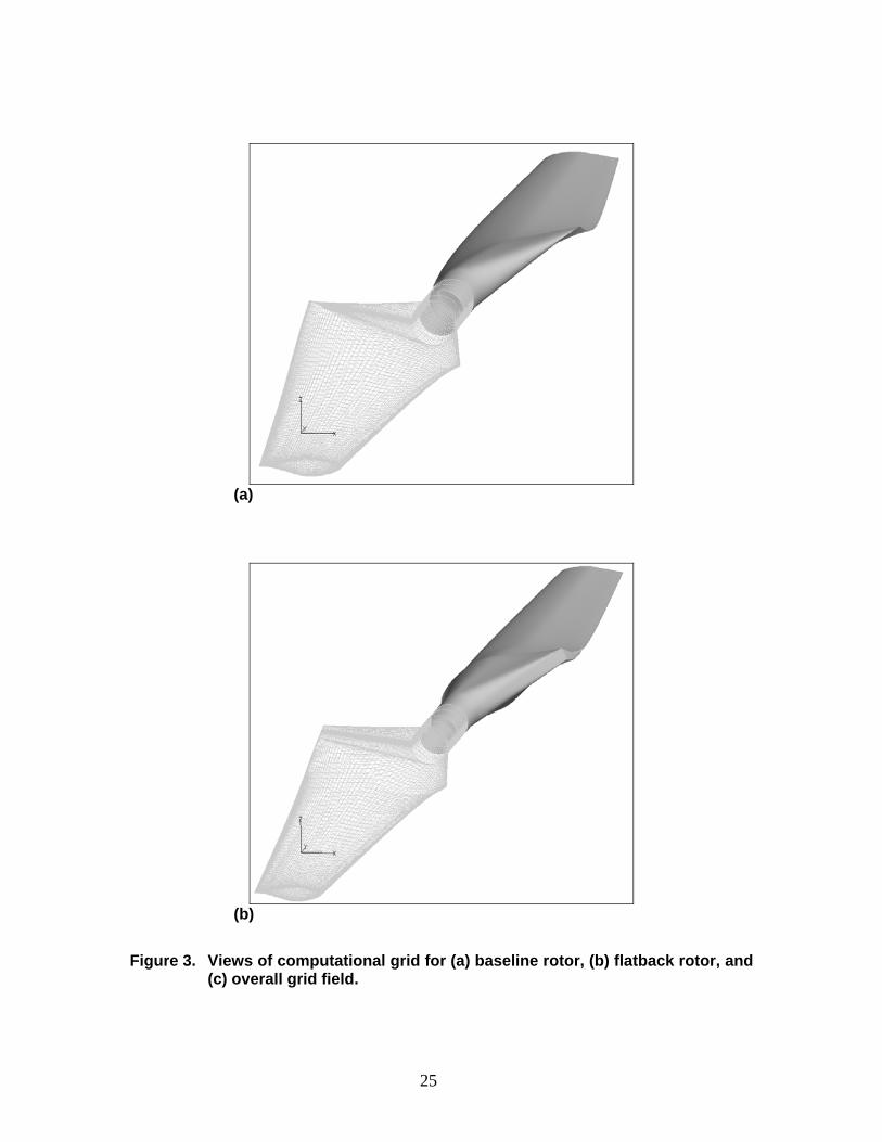
Grid Generation For this study, two O-grids are used as the nearfield grids to cover the two rotor blades as seen in Figure 3. For both rotor configurations, in both the leading-edge and the trailing-edge regions, the initial circumferential grid spacings are set at 1 × 10⁻³, and the initial wall spacing is set at 2 × 10⁻⁵ for a y+ < 1. Final mesh size for this nearfield grid including both rotor blades yields approximately 1.3 million grid points. The auto farfield grid generation in OVERFLOW is used to generate the rest of the grid field. For the baseline rotor, including the nearfield components, this results in a total of 42 grid pieces. For the flatback rotor, the total is 57 grid pieces. Both grid fields, however, contain just over 2.7 million grid points total. For all cases, the farfield is located approximately 20 unit chords or 1.5 rotor diameters away.
Results and Discussion Three wind speeds are utilized for this study: 10 m/s, 7 m/s, and 5 m/s. Due to priority of interest, the wind speed cases were conducted in descending order, thus results from the 10 m/s cases will be presented first in the following sections, followed by the 7 m/s and 5 m/s cases. Also, the dynamic simulation at each wind speed is done in two different ways. The first method is to run the simulation normally. The second method involves scaling the freestream velocity by 250% of its original value. The angular velocity is scaled the same to preserve the original tip-speed ratio. This rescaling method is used to mitigate low-Mach effects in the dynamic simulation, and thus improve solution quality without significantly altering the original flow physics. The last solution method for each wind speed is the source term formulation with low-Mach preconditioning. For brevity, the first method will be referred to as the normal dynamic solution, the second as the rescaled solution, and the third as the source term solution. In presenting the results from each of the three wind speeds, the data for the baseline turbine will be discussed first, before moving to the flatback turbine. The exception will be discussions of the torque prediction; where for concision and convenience, both the baseline and the flatback results will be presented together. For comparison to the experimental results, only the upwind data (Sequence H from the NREL/NASA-Ames Combined UAE wind tunnel study [7,15]) is used. This is because the CFD analysis does not model the tower; thus tower wake effects on the blade are not present. Tower effects are slightly noticeable in the experimental upwind data itself, but this is judged to be not significant enough to skew the comparison. For the experimental normal force coefficient and pressure coefficient data, the channel-averaged data is used. Cycle-averaged and azimuth-averaged data were also considered, but all three data sets produced nearly identical results. For the numerical solutions, only the data from the rotor blade at 0° azimuth (12 o’clock) at the final time step is used for post processing.
12
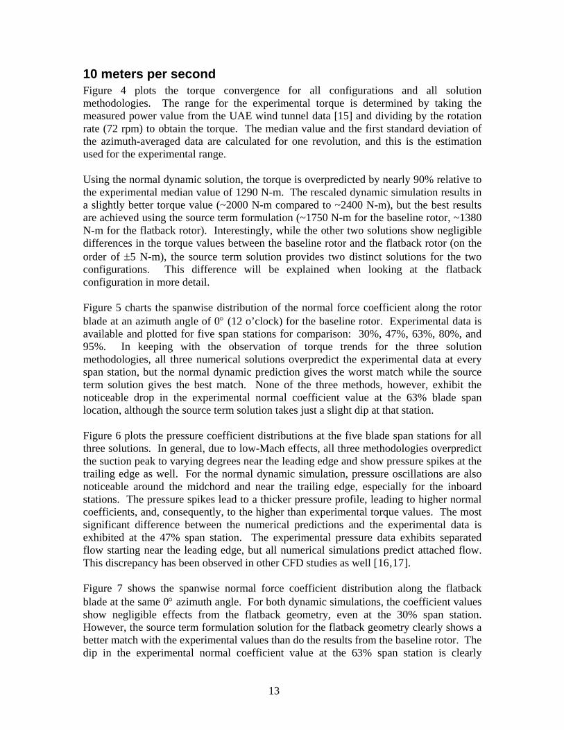
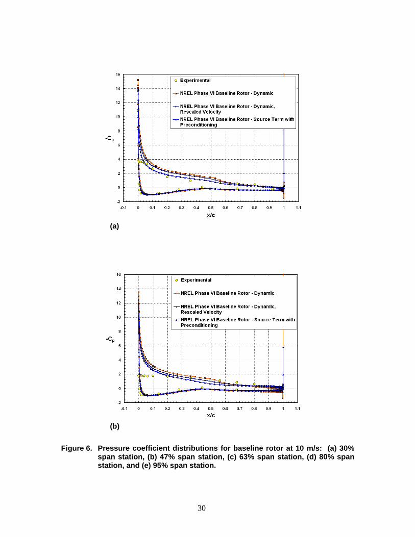
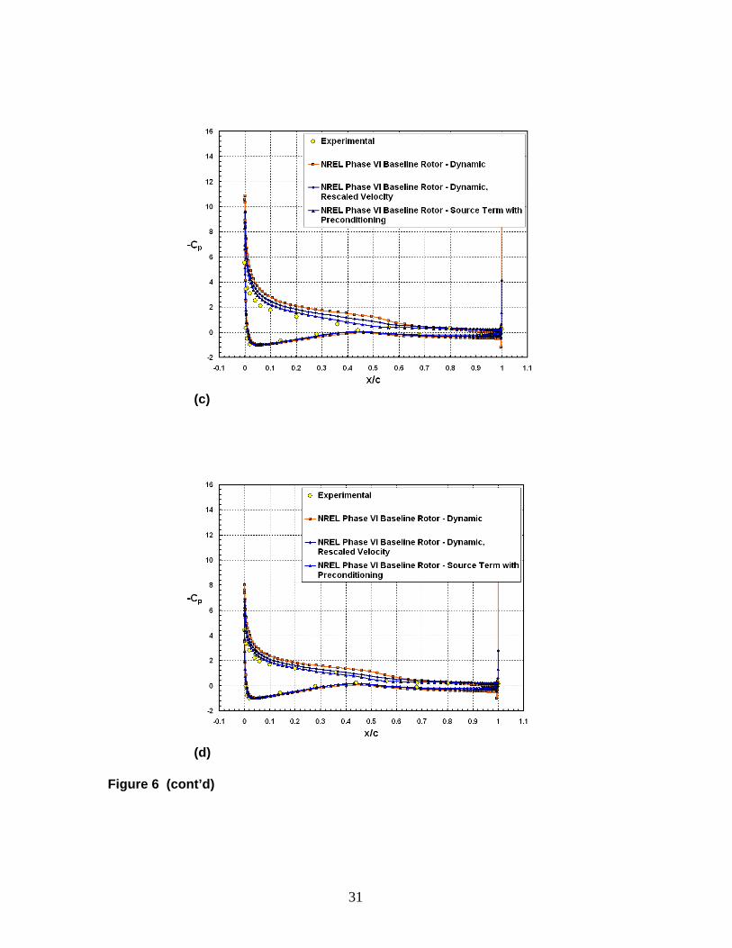
10 meters per second Figure 4 plots the torque convergence for all configurations and all solution methodologies. The range for the experimental torque is determined by taking the measured power value from the UAE wind tunnel data [15] and dividing by the rotation rate (72 rpm) to obtain the torque. The median value and the first standard deviation of the azimuth-averaged data are calculated for one revolution, and this is the estimation used for the experimental range. Using the normal dynamic solution, the torque is overpredicted by nearly 90% relative to the experimental median value of 1290 N-m. The rescaled dynamic simulation results in a slightly better torque value (~2000 N-m compared to ~2400 N-m), but the best results are achieved using the source term formulation (~1750 N-m for the baseline rotor, ~1380 N-m for the flatback rotor). Interestingly, while the other two solutions show negligible differences in the torque values between the baseline rotor and the flatback rotor (on the order of ±5 N-m), the source term solution provides two distinct solutions for the two configurations. This difference will be explained when looking at the flatback configuration in more detail. Figure 5 charts the spanwise distribution of the normal force coefficient along the rotor blade at an azimuth angle of 0° (12 o’clock) for the baseline rotor. Experimental data is available and plotted for five span stations for comparison: 30%, 47%, 63%, 80%, and 95%. In keeping with the observation of torque trends for the three solution methodologies, all three numerical solutions overpredict the experimental data at every span station, but the normal dynamic prediction gives the worst match while the source term solution gives the best match. None of the three methods, however, exhibit the noticeable drop in the experimental normal coefficient value at the 63% blade span location, although the source term solution takes just a slight dip at that station. Figure 6 plots the pressure coefficient distributions at the five blade span stations for all three solutions. In general, due to low-Mach effects, all three methodologies overpredict the suction peak to varying degrees near the leading edge and show pressure spikes at the trailing edge as well. For the normal dynamic simulation, pressure oscillations are also noticeable around the midchord and near the trailing edge, especially for the inboard stations. The pressure spikes lead to a thicker pressure profile, leading to higher normal coefficients, and, consequently, to the higher than experimental torque values. The most significant difference between the numerical predictions and the experimental data is exhibited at the 47% span station. The experimental pressure data exhibits separated flow starting near the leading edge, but all numerical simulations predict attached flow. This discrepancy has been observed in other CFD studies as well [16,17]. Figure 7 shows the spanwise normal force coefficient distribution along the flatback blade at the same 0° azimuth angle. For both dynamic simulations, the coefficient values show negligible effects from the flatback geometry, even at the 30% span station. However, the source term formulation solution for the flatback geometry clearly shows a better match with the experimental values than do the results from the baseline rotor. The dip in the experimental normal coefficient value at the 63% span station is clearly
13
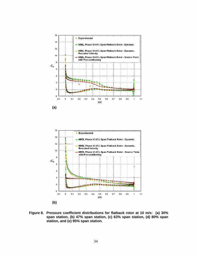
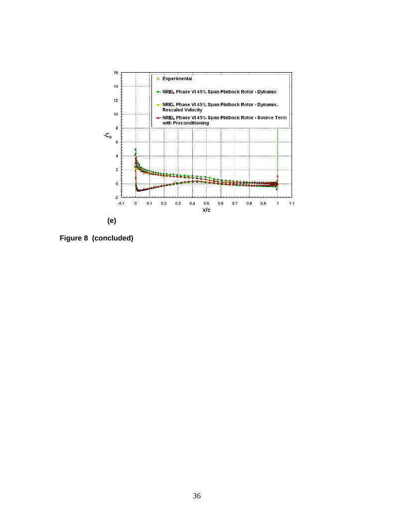
predicted by this numerical solution. The paradox here is that the flatback rotor (and not the baseline rotor) is simulating the experimental behavior more accurately. Figure 8 shows the pressure coefficient distributions at the five span stations for the flatback blade. The 30% station, as expected, shows pressure distributions different from the experimental measurements, due to the different sectional geometry. The dynamic simulations show obvious oscillations in values around the midchord of the sectional profile, where the thickness is maximum, as well as near the trailing edge. These oscillations are likely due to low-Mach number effects. At the 47% span station, the source term methodology provides an unexpected surprise. This solution now correctly predicts the leading-edge separation exhibited by the experimental data and matches the experimental pressure distribution almost exactly. Since the prediction for the baseline rotor does a poor job of matching this pressure distribution, one possible conclusion is that the sectional modifications to the inboard region of the blade, coupled with the source term methodology, are responsible for the agreement. The thicker profile increases the loading in the inboard region. This increased loading has a spanwise effect; thus the mid-span region, already close to stall at the 10 m/s wind speed, also experiences additional loading and stalls. Note that at rotor span stations 45% and greater, the sectional profiles are the same for both the flatback rotor and the baseline rotor. In Figure 9, the suction side of the baseline rotor shows flow separating near the midchord starting at the 40% span station. The flow separation point then moves slightly towards the leading edge proceeding out to the blade tip, but it never reaches the leading edge anywhere along the blade span. For the flatback rotor, again, separation around the midchord occurs starting near 40% of the span. However, leading edge separation is apparently already occurring at this point, with subsequent reattachment before separation near the midchord. This behavior is again likely due to the thickened profile and hence the increased loading of the inboard region compared to the baseline rotor. Separated flow tends to have a significant spanwise effect [17]; thus the leading edge separation is propagated along the span. The flow along the blade section roughly between 40% span and 55% span is essentially stalled. Beyond 55% span, the flow gradually recovers from stall, attaches near the leading edge, and moves the separation point gradually back towards midchord. By the 70% span station, the flow pattern regains similarity with that of the baseline rotor. Referring back to the pressure coefficient distributions of Figure 8 at the 63% span station, the source term solution matches the experimental pressure distribution better than the dynamic solutions do. Figure 9 indicates that, for the source term solution at this span station, the flow is recovering from the stalled mid-span region. This may just be coincidence, but it may also indicate that the combination of the source term solution plus effects from the flatback geometry triggers a flow phenomenon that better represents the actual flow physics of the experimental Phase VI rotor. For the actual rotor, geometry in the inboard region seems to be the prime determinant for “tripping” the separation behavior. Geometry variations between the actual Phase VI rotor and the design geometry may be the cause for the separated flow behavior of the actual rotor.
14
The 80% and 95% span station pressure distributions show the same profiles as for the baseline rotor for the respective solution methodologies. Overall, source term formulation with low-Mach preconditioning provides the best agreement with experimental data.
7 meters per second Figure 10 shows the torque convergence history for all 7 m/s test cases. The general trends observed for the 10 m/s cases apply here as well. No significant differences in the predicted torque values are observed between the baseline rotor and the flatback rotor for all three solution methodologies (they agree within ±5 N-m). For the dynamic simulations, the overprediction of the torque is less severe compared to the 10 m/s test cases, roughly about 25% over the experimental median torque value for the normal dynamic simulations (~990 N-m) and about 19% overprediction for the dynamic rescaled velocity simulations (~940 N-m). Again, the source term formulation provides the best prediction, converging to about 815 N-m, compared to the experimental mean of 790 N-m. Unlike the 10 m/s case, however, the source term formulation converges to essentially the same torque value for both rotor configurations. For the baseline rotor, the spanwise normal force coefficients are plotted in Figure 11. Again, the dynamic solutions predict essentially the same coefficient values along the span while the source term solution better matches the experimental data. All solutions overpredict the experimental normal force coefficient at each span station. The source term solution, however, best predicts the lower normal coefficient value at the 30% span station. The pressure coefficient distributions are plotted in Figure 12. The dynamic solutions again tend to greatly overpredict the suction peak near the leading edge, while also showing a pressure spike and small oscillations near the trailing edge. The source term solution shows the same traits but to a lesser degree, with no pressure oscillations as a result of the application of low-Mach preconditioning. This means the source term solution, in general, shows a “thinner” pressure profile, so the resulting normal force coefficients are more in line with the experimental values. The spanwise normal force coefficients for the flatback rotor are plotted in Figure 13. As was the case for the dynamic solutions of 10 m/s flow condition, the flatback geometry produces no significant variation in the spanwise distribution compared to the baseline rotor. For the source term solution, the numerical prediction is slightly better at the 30% span station compared to the respective baseline rotor solution. This is likely due to coincidence, since the pressure distributions are expected to be very different between the two rotor configurations, but each may integrate to nearly the same normal force coefficient. Again, only the source term solution follows the general curve of the experimental spanwise distribution of the normal force coefficient. Figure 14 plots the distributions of the pressure coefficients along each of the five spanwise stations for the flatback rotor. For all the solutions except those at the 30% span station, the pressure profiles differ little from the baseline rotor. What are more noticeable for the dynamic solutions, however, are the pressure oscillations, especially
15
near the trailing edge. Pressure oscillations are also noticeable near the leading edge for the outboard stations. For the 30% span station, the flow has apparently separated near the leading edge on the upper surface but has re-attached itself within 2% of the local chord. The pressure gradient is then favorable until it reaches 33% of the chord. There, it steeply changes over to an adverse pressure gradient that builds to the trailing edge. The apparent separation near the leading edge for the CFD results may be accurate, but for a different reason: modeling limitations. All the numerical test cases assume fully turbulent flow, but the flow conditions may dictate that a region should really be laminar. Thus the dip in pressure after the suction peak may indicate an exaggerated effect of using a turbulence model to simulate what could be a laminar separation bubble. Figure 15 compares the velocity magnitude on the suction side of both rotor configurations. Except for the inboard portion around 30% span, the flow patterns are essentially the same. The flow remains attached along the whole blade for both rotor configurations although thickening of the boundary layer aft of each sectional maximum thickness is noticeable.
5 meters per second The torque convergence histories for the 5 m/s case are plotted in Figure 16. For this case, only the normal dynamic simulation and the source term simulation are used, since the rescaled dynamic simulation produces a lesser improvement at these lower wind speeds. The mean experimental torque value is calculated to be 295 N-m. The dynamic solution predicts a torque of approximately 400 N-m for both rotor configurations while the source term solution predicts a value of about 160 N-m. Thus the dynamic solution overpredicts by about 36% while the source term solution underpredicts by about 46%. Given that in all the previous flow conditions, the source term solution has consistently yielded the best results, the larger discrepancy in this case may be surprising. However, the solution is only as good as the model, and for this case, the model may be inadequate. This is because at 5 m/s, a substantial portion of the flow over the rotor may be laminar; thus modeling the flow as fully turbulent would be unsuitable at best. However, laminar flow over the rotor can be expected to yield a higher torque value than turbulent flow, so the results here are still consistent. The spanwise normal force coefficients for the baseline rotor are plotted in Figure 17. The dynamic solution overpredicts the experimental values at every span station, while the source term solution underpredicts the inboard stations but slightly overpredicts the outboard stations. At the 63% span station, the source term solution essentially agrees exactly with the experimental normal force coefficient. The larger discrepancies for the inboard data result in the underprediction of the experimental torque. Pressure coefficient distributions for the baseline rotor are plotted in Figure 18. Immediately noticeable are the pressure oscillations along the blade section at all span locations for the dynamic solution, whereas the source term solution is fairly smooth. This speaks to the utility of having low-Mach preconditioning – it improves both the convergence value and the quality of the solution. In general, the dynamic solution
16

overpredicts the pressure distribution along the suction side but agrees very well with the pressure side at all span locations. The source term solution results in a mixed bag. For the inboard stations, along the suction side, the source term solution underpredicts the forward half but overpredicts the rear half of the section profile. Along the pressure side, the forward half agrees well, but the solution, from midchord to trailing edge, overpredicts the pressure deficit. This overprediction, on the aft half of the inboard blade sections along both the suction and pressure side surfaces, means the resulting pressure profile for the aft half is offset on the vertical axis. This may be an effect of using turbulence to model what may be laminar flow in the experimental data. The experimental pressure profiles do suggest that the forward half of the sectional airfoils, up to 40% of the local chord, may be experiencing laminar flow instead of turbulent flow. This suggests transition modeling is necessary at this low wind speed. The spanwise distribution of the normal force coefficient for the flatback rotor is plotted in Figure 19. Very small changes compared to the baseline rotor are noticeable for both solutions. That these results are from the flatback rotor instead of the baseline rotor would be difficult to discern from this plot alone. Looking at the pressure coefficient distributions (see Figure 20), however, the flatback effect is very obvious for the 30% span station. On the suction side, a favorable pressure gradient region exists for over 40% of the chord before quickly changing over into an adverse pressure gradient. Again, although the pressure profiles are vastly different at this span station between the flatback rotor and the baseline rotor, integration of the area within the profiles yields essentially the same normal force coefficient value. Overall, the dynamic solution shows poor quality for all blade stations, whereas the source term solution yields smooth distributions, but with apparently the same type of laminar-versus-turbulent discrepancies as noted for the baseline rotor. Smooth plots of the velocity magnitude along the suction-side surface of both rotors are shown in Figure 21. The flow over the two configurations is very similar. Some separation exists around midchord in the inboard shank region, but otherwise, the flow over the blades remains attached, with a small thickening of the boundary layer near the trailing edge in the outboard regions. These flow traits will be better illustrated in the flow-visualization discussion presented below.
Flow visualization Cross-sectional views of the velocity magnitude field are shown and compared for the baseline rotor and the flatback rotor for several blade stations for all three wind speeds in Figure 22 – Figure 24. For the 10 m/s case, both rotors show midchord separation for the inboard stations. However, around the 45% blade station, the flatback rotor shows complete separation on the suction side, while the baseline rotor maintains the midchord separation trend. As was shown in Figure 9, the mid-span region of the flatback rotor is completely stalled, but the baseline rotor maintains the midchord separation (aft of section maximum thickness) essentially along the complete blade span. By the 63% blade station, the flatback rotor has partially recovered from stall, but separation still occurs forward of maximum thickness, in contrast to the baseline blade at the same
17

station. At 80% and 95% blade stations, the flow physics over both blades becomes very similar again, with separation occurring aft of maximum thickness. For the 7 m/s case (Figure 23), midchord separation occurs for the inboard shank region. However, by the 25% blade station, the baseline rotor shows completely attached flow, whereas the flatback rotor still shows separation just a bit aft of maximum airfoil thickness. However, by the 30% span station, the flatback rotor also indicates attached flow, but boundary layer thickening prior to separation at the blunt trailing edge is noticeable compared to the baseline blade. For solutions outboard of this point, both blades show similar flow physics with attached flow but thickening of the boundary layer towards the trailing edge. For the 5 m/s case (Figure 24), separation occurs for the inboard shank region, but by the 25% blade station, both blades show fully attached flow. In fact, for the flatback rotor, the flow leaves the blunt trailing edge smoothly, apparently moving the Kutta condition downstream of the trailing edge and elongating the effective chord of the blade section. This is noticeable for the 30% blade station as well. Otherwise, the flow over both blade designs at this wind speed is fully attached, with minor thickening of the boundary layer near the trailing edge in the outboard region.
Some further analysis To further explore the differences between the results for the baseline and the flatback configurations at 10 m/s, where the flatback configuration yielded pressure distributions more in line with the experimental data, additional analysis was conducted. To accomplish this, a third blade geometry is generated and analyzed. This blade geometry is designed to fall in between the previous baseline and flatback configurations. For the third configuration, the S809 profile at the 25% span station has been modified to have the identical camber as the S809 but a maximum thickness-to-chord ratio of 40% (identical to the flatback configuration) and to have a sharp trailing edge (identical to the baseline configuration). This airfoil modification at the 25% span station is then blended, so that by the 45% span station, this airfoil thickness modification has blended back to the original baseline blade schedule. This configuration will be referred to as the thick blade. Figure 25 shows a profile comparison of all three airfoils as well as a tunnel view of the thick blade design. The purpose of the thick blade is to evaluate separately the effects of increasing the maximum thickness-to-chord ratio and the trailing-edge thickness for the inboard portion of the blade. For this analysis, only solutions from the source term formulation with low-Mach preconditioning are used because this method consistently yielded the best results. Figure 26 shows the torque convergence histories for all three rotor configurations at 7 m/s and 10 m/s. At 7 m/s, the thick rotor almost identically follows the convergence path of the flatback rotor to a mean torque value of 800 N-m. This is 15 N-m lower than the predicted torques from both the baseline rotor and the flatback rotor but agrees closer to the experimental mean of 790 N-m. Although thickening the blade results in this slight
18
loss in torque compared to the baseline rotor, adding a flatback tail to the thick rotor does rectify this loss. At 10 m/s, the thick rotor converges much faster than both the baseline and the flatback rotors to a mean torque value of 1750 N-m, the same value as for the baseline rotor. Figure 27 shows the spanwise normal force coefficient and the nondimensional torque load distributions for all three blade configurations at 7 m/s and 10 m/s. The torque load distribution plots better demonstrate the increased loading moving from inboard of the blade to the blade tip. Looking at the torque distribution for the 7 m/s result, the thick rotor consistently has lower loading along the inboard portion of the blade compared to the baseline rotor but has slightly higher loading in the outboard region. For the flatback rotor, compared to the baseline rotor, the general trend is the same except there is a significant increase in loading around the 15% span station. What is more significant, however, is that the flatback rotor consistently shows higher loading along the complete span compared to the thick rotor. This demonstrates that, given the 40% thickness for both rotors, having a flatback trailing edge offers noticeable advantages over a sharp trailing edge, especially along the inboard portion of the blade. For the 10 m/s case, the results are more mixed. From the normal coefficient distribution plot, comparing the thick rotor to the baseline rotor, again, the thick rotor exhibits higher loading in the outboard region. In the inboard region, however, the thick rotor starts with a lower loading but shows a more rapid loading increase before dipping at the 25% span station. The effect is as if the load curve for the thick rotor has been shifted right compared to the baseline rotor. The flatback rotor, as previously noted, shows some interesting behavior. Unlike the other two blades, the flatback blade almost has a loading plateau in the inboard region according to the normal coefficient distribution. Overall, in the inboard region, the flatback rotor shows higher loading compared to the thick rotor and the baseline rotor, but, at a wind speed of 10 m/s, this higher loading also triggers a significant loss in loading in the outboard region between approximately 45% and 75% of the blade span. Looking at the torque distribution plot, the flatback blade in the inboard region has a loading comparable or slightly higher than the baseline blade. However, at the 45% span station, the flatback blade has a higher loading than both the baseline blade and the thick blade. This higher loading is apparently what causes the flow to separate in the mid-span section compared to the other two configurations. At both wind speeds and for all rotor configurations, from the normal force coefficient distributions, there is a noticeable drop in loading around the break point (25% span station) of the blade. This may be due to the abruptness of the break point along the trailing edge of the blade, which may be causing the spanwise flow to separate around this region. For the baseline blade, the loading drops around the 20% span station, whereas the thick blade and the flatback blade loadings both drop around the 25% span station. However, the baseline blade also shows a significant increase in loading after dropping to a minimum. The significance of this behavior may explain the behavior observed in the actual Phase VI rotor. Perhaps due to integration and blending of the blade shaft which results in a thicker inboard profile section than the design profile, the loading decrease for the actual rotor occurs closer to the 25% break point station than the
19
20% span station indicated by the computational results. The loading then increases significantly, just as the baseline computational results indicate, to a peak loading that is comparable to the flatback blade. And as noted before, this high loading leads to mid-span separation at 10 m/s for the flatback blade. This loading behavior might explain the discrepancy between the experimental results and the computational results for the baseline rotor at 10 m/s. The pressure coefficient distributions at several span stations for all three rotor configurations at 7 m/s are plotted in Figure 28. In the inboard region, due to blade profile differences, the baseline rotor tends to have the highest suction peaks on the blade suction side. The flatback rotor develops a noticeable suction peak faster than the thick rotor moving outwards along the span. Outward of the 45% span station, because all three rotors revert to the same blade geometry, the pressure distributions all become essentially identical. Figure 29 shows the pressure distributions for all three rotor configurations at 10 m/s. At this wind speed, the thick rotor and the flatback rotor both have similar pressure developments in the inboard region. However, at the 45% span station, the flatback rotor begins to lose some normal force due to flow separation, whereas the thick rotor has the same pressure profile as the baseline rotor. The flatback rotor does not recover the same pressure distributions as the other two rotors until around the 70% span station. These plots give a better picture of how the flatback rotor increases the loading in the inboard region just enough to cause mid-span stall. On a side note, the twist and planform distributions for all three rotor configurations are identical to that of the Phase VI blade, and were optimized for this baseline blade with the S809 section shape. However, changes in the blade load distribution caused by the thickening of the inboard sections (flatback and thick blade) and trailing edges (flatback blade) clearly necessitate a re-optimization of both the twist and planform distributions. The results presented here apparently indicate that the higher loading generated by the flatback sections requires the use of more twist in the inboard region of the blade and perhaps a rounding of the sharp break point at the 25% span station.
Conclusions The objective of this study is to analyze the effects of modifying the inboard portion of the NREL Phase VI rotor with a thickened, flatback version of the S809 design airfoil. The motivation for using a thicker airfoil design with a blunt trailing edge is to alleviate structural constraints while reducing blade weight and maintaining the power performance of the rotor. This study focuses on the aerodynamic effects from these modifications which contribute to torque, and hence, power performance. To this end, two rotor configurations, a baseline configuration and a flatback configuration, are used to study these effects at three different wind speeds. Three methods of simulating the flow are utilized, including
20
a normal dynamic simulation with moving rotor grids, a velocity-scaled dynamic solution which partially mitigates low-Mach effects, and a pseudo-steady-state source term simulation which benefits from having a low-Mach preconditioning algorithm applied. In general, the source term solution produces the best results. While not necessarily agreeing with the experimental data exactly, the source term results best matches the experimental results for the baseline rotor. The normal dynamic solution provides the poorest results, possibly due to low-Mach effects. With one particular exception noted below, each solution method produces essentially the same torque value for both rotor configurations, with most variations falling within ±5 N-m. The predicted flow physics are different, especially in the inboard regions, but these differences do not translate to significant differences in the distributions of the spanwise normal force coefficients or the resulting torque values. For the lowest wind speed of 5 m/s, the source term solution underpredicts the experimental torque range. However, analysis of the pressure coefficient distributions at the five spanwise blade stations does suggest up to 40% of the local flow over each section may be laminar. However, all solutions assumed fully turbulent flow for all the wind speeds considered. Thus one area of additional research is to re-examine this case with a specified or predicted transition line along the blade span. Another possible source for the discrepancy may be the deviations in the experimental freestream flow [6] which the source term formulation is unable to capture. For the 7 m/s case, the source term solution falls within the experimental range, matching very closely with the experimental mean torque value to within 4%. Separation is observed in the inboard shank region for both rotor configurations, but otherwise the flow remains completely attached. The flow at this wind speed is relatively well-behaved and explains the good agreement in pressure and normal force coefficient distributions between the source term solutions and the experiment. For the 10 m/s case, the source term solution provides two distinct solutions to the two rotor configurations. The flatback solution shows a noticeable drop in torque compared to the baseline solution, but this decrease paradoxically makes the flatback solution fall in line with the experimental results. The baseline solution shows midchord separation essentially along the entire blade span, but the flatback solution reveals that a region around the mid-span of the blade is stalled, with leading-edge flow separation. This flow feature produces pressure coefficient distributions, and consequently, the normal force coefficients, around the mid-span that matches the experimental data almost exactly. This is a unique effect which has not been observed in other CFD studies, and is likely due to spanwise effects from the increased loading in the inboard region resulting from the flatback blade sections compared to the baseline rotor. This study shows that using a flatback rotor did reduce the torque compared to the baseline rotor at all wind speeds. However, this outcome is mitigated by several factors. For one, the twist and planform distributions for all rotor configurations are based on and originally optimized for the NREL Phase VI blade with the S809 airfoil section shape.
21
However, changes in the blade load distribution caused by the thickening of the inboard sections and trailing edges require a new analysis of both the twist and planform specifications. For example, the results presented here appear to indicate that the higher loading generated by the flatback sections requires more twist in the inboard region of the blade. Another mitigating factor is that thickening the airfoil profile to 40% is very aggressive aerodynamically; a somewhat thinner airfoil may be sufficient to satisfy structural requirements. A final mitigating factor is that given the 40% maximum thickness, the 10% trailing edge flatback is rather thin. Standish and van Dam [5] previously observed that an airfoil thickness-to-flatback ratio of 2-to-1 may be optimal; thus the flatback modification corresponding to the present 40% thickness blade profile should ideally be closer to 20% than 10%. Therefore, the current flatback blade is not particularly optimized for anything but is simply used as a comparison to the baseline rotor. A last factor to consider is that designing a flatback rotor does not entail being limited to modifying existing designs. Beyond choosing to use a thicker, flatback profile, other parameters such as twist distribution and profile blending between blade sections will also factor into the design of an optimized flatback rotor. What this study does prove is that a thick, flatback blade profile is viable as a bridge to connect structural requirements with aerodynamic performance in designing future wind turbine rotors.
22
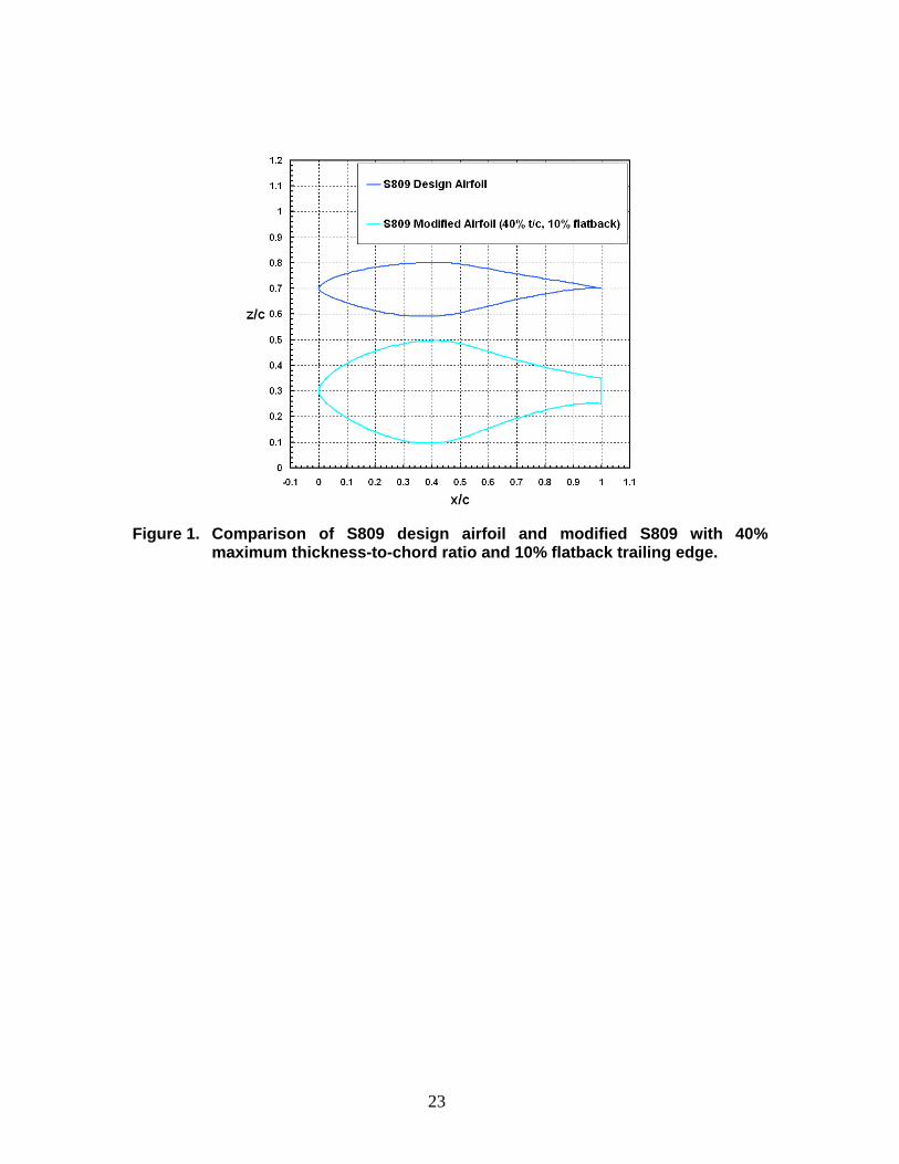
Figure 1. Comparison of S809 design airfoil and modified S809 with 40%
maximum thickness-to-chord ratio and 10% flatback trailing edge.
23
(a)
(b)
Figure 2. Tunnel views of geometric schedules for (a) baseline rotor blade, and
(b) flatback rotor blade.
24
(a)
(b)
Figure 3. Views of computational grid for (a) baseline rotor, (b) flatback rotor, and
(c) overall grid field.
25

(c)
Figure 3 (concluded)
26

(a)
(b)
Figure 4, Torque convergence histories for 10 m/s cases: (a) normal dynamic
simulations, (b) dynamic simulations with 250% scaled velocities, and (c) source term with low-Mach preconditioning simulations.
27

(c)
Figure 4 (concluded)
28
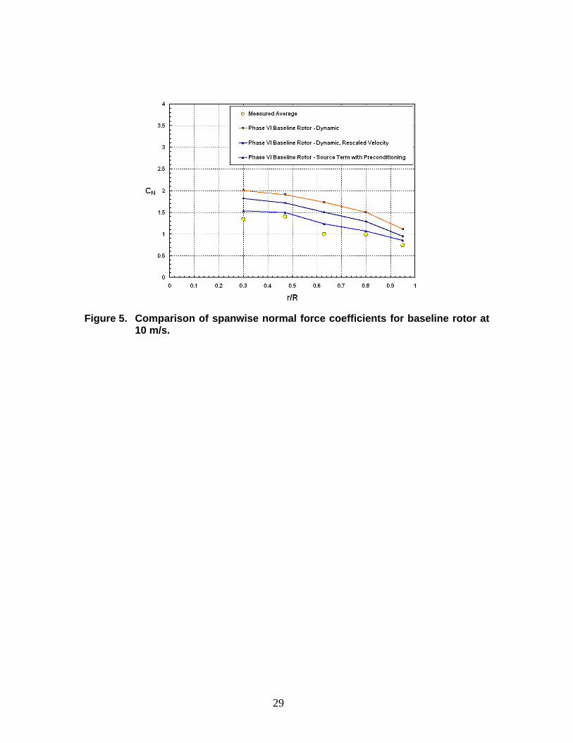
Figure 5. Comparison of spanwise normal force coefficients for baseline rotor at
10 m/s.
29
(a)
(b)
Figure 6. Pressure coefficient distributions for baseline rotor at 10 m/s: (a) 30%
span station, (b) 47% span station, (c) 63% span station, (d) 80% span station, and (e) 95% span station.
30
(c)
(d)
Figure 6 (cont’d)
31

(e)
Figure 6 (concluded)
32
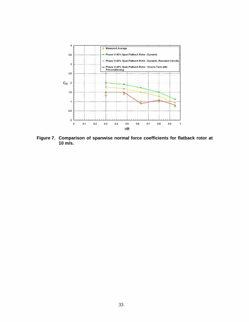
Figure 7. Comparison of spanwise normal force coefficients for flatback rotor at
10 m/s.
33
(a)
(b)
Figure 8. Pressure coefficient distributions for flatback rotor at 10 m/s: (a) 30%
span station, (b) 47% span station, (c) 63% span station, (d) 80% span station, and (e) 95% span station.
34

(c)
(d)
Figure 8 (cont’d)
35
(e)
Figure 8 (concluded)
36

(a)
(b)
Figure 9. Smooth plots of velocity magnitude on suction side surface of rotor
configurations at 10 m/s for (a) baseline rotor, and (b) flatback rotor. Black lines refer to span stations where Cp distributions are compared. Red line refers to 45% span station where blade geometries for both configurations become the same. Solutions obtained from source term with low-Mach preconditioning simulation.
37
(a)
(b)
Figure 10. Torque convergence histories for 7 m/s cases: (a) normal dynamic
simulations, (b) dynamic simulations with 250% scaled velocities, and (c) source term with low-Mach preconditioning simulations.
38

(c)
Figure 10 (concluded)
39
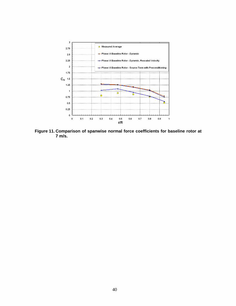
Figure 11. Comparison of spanwise normal force coefficients for baseline rotor at
7 m/s.
40

(a)
(b)
Figure 12. Pressure coefficient distributions for baseline rotor at 7 m/s: (a) 30%
span station, (b) 47% span station, (c) 63% span station, (d) 80% span station, and (e) 95% span station.
41

(c)
(d)
Figure 12 (cont’d)
42
(e)
Figure 12 (concluded)
43
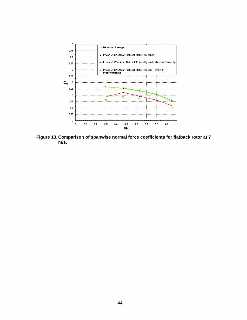
Figure 13. Comparison of spanwise normal force coefficients for flatback rotor at 7
m/s.
44
(a)
(b)
Figure 14. Pressure coefficient distributions for flatback rotor at 7 m/s: (a) 30%
span station, (b) 47% span station, (c) 63% span station, (d) 80% span station, and (e) 95% span station.
45

(c)
(d)
Figure 14 (cont’d)
46

(e)
Figure 14 (concluded)
47

(a)
(b)
Figure 15. Smooth plots of velocity magnitude on suction side surface of rotor configurations at 7 m/s for (a) baseline rotor, and (b) flatback rotor. Black lines refer to span stations where Cp distributions are compared. Red line refers to 45% span station where blade geometries for both configurations become the same. Solutions obtained from source term with low-Mach preconditioning simulation.
48

(a)
(b)
Figure 16. Torque convergence histories for 5 m/s cases: (a) normal dynamic
simulations, and (b) source term with low-Mach preconditioning simulations.
49

Figure 17. Comparison of spanwise normal force coefficients for baseline rotor at
5 m/s.
50
(a)
(b)
Figure 18. Pressure coefficient distributions for baseline rotor at 5 m/s: (a) 30%
span station, (b) 47% span station, (c) 63% span station, (d) 80% span station, and (e) 95% span station.
51

(c)
(d)
Figure 18 (cont’d)
52
(e)
Figure 18 (concluded)
53
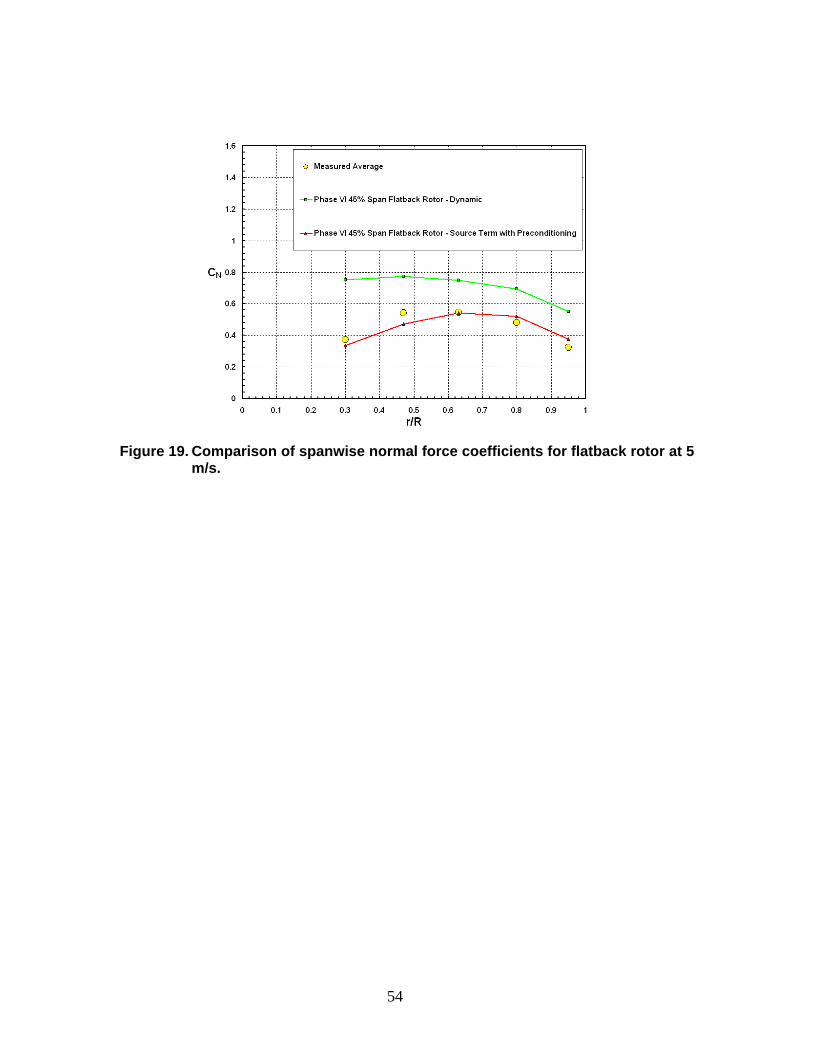
Figure 19. Comparison of spanwise normal force coefficients for flatback rotor at 5
m/s.
54

(a)
(b)
Figure 20. Pressure coefficient distributions for flatback rotor at 5 m/s: (a) 30%
span station, (b) 47% span station, (c) 63% span station, (d) 80% span station, and (e) 95% span station.
55

(c)
(d)
Figure 20 (cont’d)
56
(e)
Figure 20 (concluded)
57
58
(a)
(b)
Figure 21. Smooth plots of velocity magnitude on suction side surface of rotor configurations at 5 m/s for (a) baseline rotor, and (b) flatback rotor. Black lines refer to span stations where Cp distributions are compared. Red line refers to 45% span station where blade geometries for both configurations become the same. Solutions obtained from source term with low-Mach preconditioning simulation.
(a)
(b)
(c) Figure 22. Comparison of velocity magnitude smooth contours over rotor
configurations at 10 m/s for spanwise stations at (a) 5%, (b) 15%, (c) 25%, (d) 30%, (e) 45%, (f) 47%, (g) 63%, (h) 80%, and (i) 95%. Left-hand side is baseline rotor, and right-hand side is flatback rotor.
59
(d)
(e)
(f) Figure 22 (cont’d)
60

(g)
(h)
(i) Figure 22 (concluded)
61

(a)
(b)
(c) Figure 23. Comparison of velocity magnitude smooth contours over rotor
configurations at 7 m/s for spanwise stations at (a) 5%, (b) 15%, (c) 25%, (d) 30%, (e) 45%, (f) 47%, (g) 63%, (h) 80%, and (i) 95%. Left-hand side is baseline rotor, and right-hand side is flatback rotor.
62
(d)
(e)
(f) Figure 23 (cont’d)
63

(g)
(h)
(i) Figure 23 (concluded)
64

(a)
(b)
(c) Figure 24. Comparison of velocity magnitude smooth contours over rotor
configurations at 5 m/s for spanwise stations at (a) 5%, (b) 15%, (c) 25%, (d) 30%, (e) 45%, (f) 47%, (g) 63%, (h) 80%, and (i) 95%. Left-hand side is baseline rotor, and right-hand side is flatback rotor.
65

(d)
(e)
(f) Figure 24 (cont’d)
66

(g)
(h)
(i) Figure 24 (concluded)
67
(a)
(b)
Figure 25. Comparison of thickened 40% t/c S809 airfoil with sharp trailing edge to previous airfoil geometries; (a) profile comparison, and (b) tunnel view of resultant blade.
68

(a)
(b)
Figure 26. Torque convergence histories of all three rotor configurations at (a) 7 m/s, and (b) 10 m/s. All solutions obtained using source term formulation with low-Mach preconditioning.
69
70
(a)
(b)
Figure 27. Comparison of blade geometry effects on the spanwise normal force
coefficient and the nondimensional torque loading distributions for the (a) 7 m/s, and (b) 10 m/s test cases. All solutions obtained using source term formulation with low-Mach preconditioning.
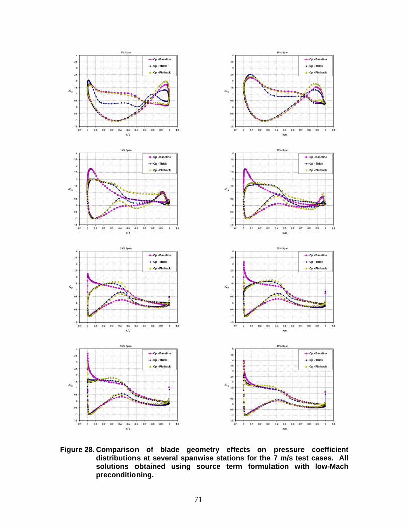
Figure 28. Comparison of blade geometry effects on pressure coefficient
distributions at several spanwise stations for the 7 m/s test cases. All solutions obtained using source term formulation with low-Mach preconditioning.
71
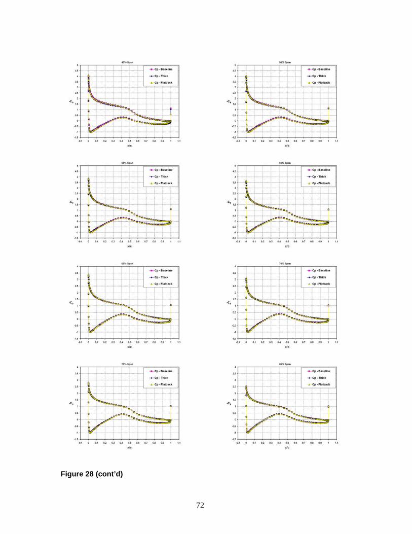
igure 28 (cont’d) F
72

igure 28 (concluded)
F
73
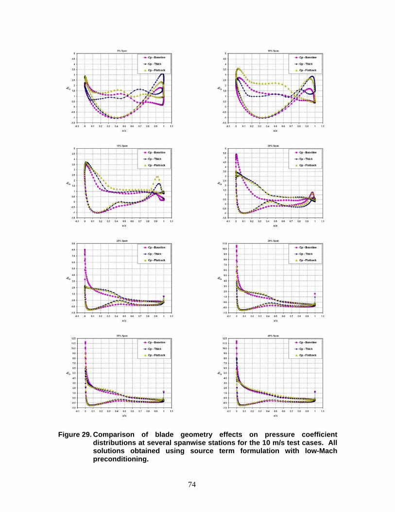
Figure 29. Comparison of blade geometry effects on pressure coefficient distributions at several spanwise stations for the 10 m/s test cases. All solutions obtained using source term formulation with low-Mach preconditioning.
74

Figure 29 (cont’d)
75
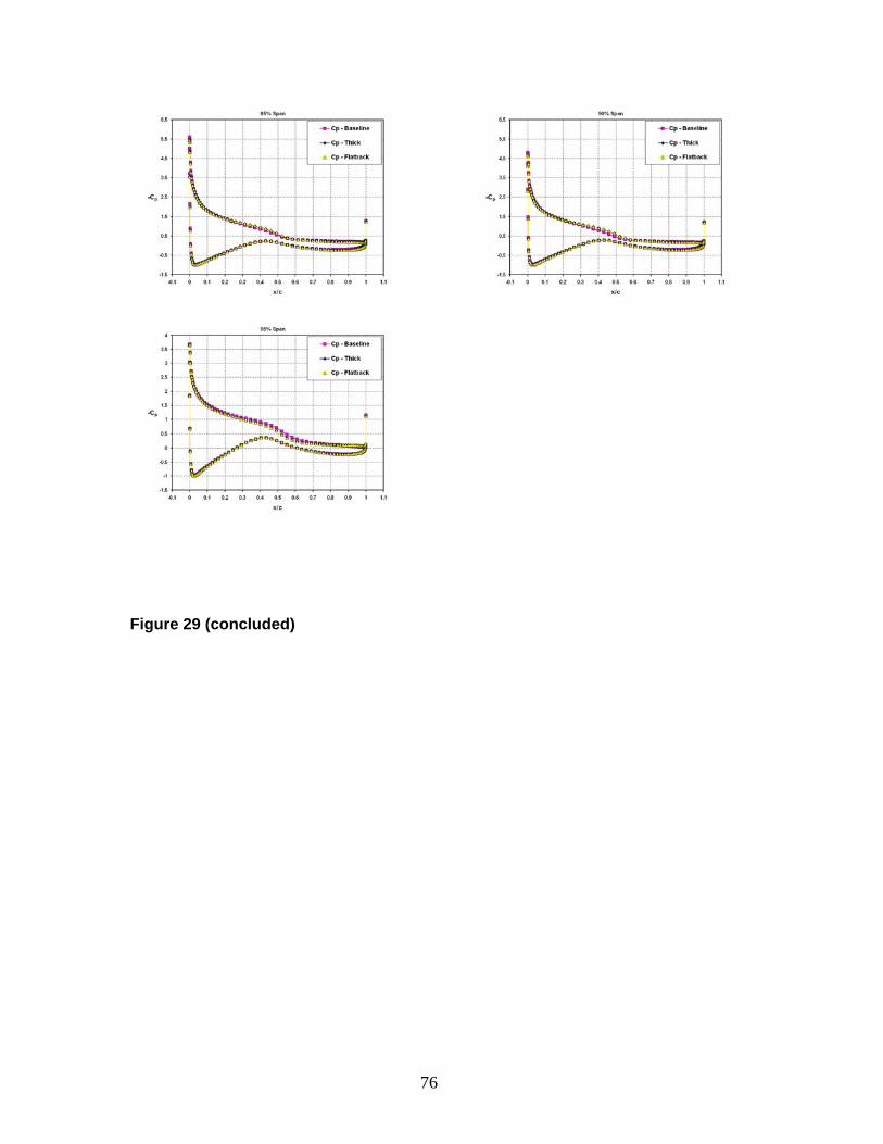
Figure 29 (concluded)
76
References 1 TPI Composites, "Parametric Study for Large Wind Turbine Blades," SAND2002-
2519, 2002. 2 TPI Composites, "Cost Study for Large Wind Turbine Blades," SAND2003-1428,
2003. 3 TPI Composites, "Innovative Design Approaches for Large Wind Turbine Blades,"
SAND2003-0723, 2003. 4 TPI Composites, "Innovative Design Approaches for Large Wind Turbine Blades–
Final Report," SAND2004-0074, 2004. 5 Standish, K.J., and van Dam, C.P., "Aerodynamic Analysis of Blunt Trailing Edge
Airfoils," Journal of Solar Energy Engineering, Vol. 125, 2003, pp. 479-487. 6 Simms, D., Schreck, S., Hand, M., and Fingersh, L.J., "NREL Unsteady
Aerodynamics Experiment in the NASA-Ames Wind Tunnel: A Comparison of Predictions to Measurements," NREL/TP-500-29494, June 2001.
7 Hand, M.M., Simms, D.A., Fingersh, L.J., Jager, D.W., Cotrell, J.R., Schreck, S.J.,
Larwood, S.M., "Unsteady Aerodynamics Experiment Phase VI: Wind Tunnel Test Configurations and Available Data Campaigns," NREL/TP-500-29955, Dec. 2001.
8 Giguère, P., and Selig, M.S., "Design of a Tapered and Twisted Blade for the
NREL Combined Experiment Rotor," NREL/SR-500-26173, Apr. 1999. 9 Buning, P.G., Jespersen, D.C., Pulliam, T.H., Chan, W.M., Slotnick, J.P., Krist,
S.E., and Renze, K.J., OVERFLOW User’s Manual, Version 1.8, Feb. 1998. 10 Pulliam, T.H., and Steger, J.L., "Implicit Finite Difference Simulations of Three-
Dimensional Compressible Flow," AIAA Journal, Vol. 18, No. 2, 1989, pp. 159–167.
11 Spalart, P.R., and Allmaras, S.R., "A One-Equation Turbulence Model for
Aerodynamic Flows," AIAA Paper 92-0439, Jan. 1992. 12 Jespersen, D., Pulliam, T., and Buning, P., "Recent Enhancements to
OVERFLOW," AIAA Paper 97-0644, Jan. 1997. 13 Chao, D.D., and van Dam, C.P., "Wing Drag Prediction and Decomposition,"
AIAA Paper 2004-5074, Aug. 2004.
77
78
14 Chan, W.M., and Buning, P.G., "User’s Manual for FOMOCO Utilities – Force and
Moment Computation Tools for Overset Grids," NASA TM 110408, July 1996. 15 www.nrel.gov/uaewtdata, contact [email protected]. 16 Sorensen, N.N., Michelsen, J.A., and Schreck, S., "Navier-Stokes Predictions of the
NREL Phase VI Rotor in the NASA Ames 80 ft × 120 ft Wind Tunnel," Wind Energy, Vol. 5, 2002, pp. 151-169.
17 Duque, E.P.N, Burklund, M.D., and Johnson, W., "Navier-Stokes and
Comprehensive Analysis Performance Predictions of the NREL Phase VI Experiment," Journal of Solar Energy Engineering, Vol. 125, Nov. 2003, pp. 457-467.

DISTRIBUTION: Tom Acker Northern Arizona University PO Box 15600 Flagstaff, AZ 86011-5600 Ian Baring-Gould NREL/NWTC 1617 Cole Boulevard MS 3811 Golden, CO 80401 Keith Bennett U.S. Department of Energy Golden Field Office 1617 Cole Boulevard Golden, CO 80401-3393 Karl Bergey University of Oklahoma Aerospace Engineering Dept. Norman, OK 73069 Mike Bergey Bergey Wind Power Company 2200 Industrial Blvd. Norman, OK 73069 Derek Berry TPI Composites, Inc. 373 Market Street Warren, RI 02885-0328 Gunjit Bir NREL/NWTC 1617 Cole Boulevard MS 3811 Golden, CO 80401 Marshall Buhl NREL/NWTC 1617 Cole Boulevard MS 3811 Golden, CO 80401
C.P. Sandy Butterfield NREL/NWTC 1617 Cole Boulevard MS 3811 Golden, CO 80401 Garrett Bywaters Northern Power Systems 182 Mad River Park Waitsfield, VT 05673 Doug Cairns Montana State University Dept. of Mechanical & Industrial Eng. College of Engineering PO Box 173800 Bozeman, MT 59717-3800 David Calley Southwest Windpower 1801 West Route 66 Flagstaff, AZ 86001 Larry Carr NASA Ames Research Center 24285 Summerhill Ave. Los Altos, CA 94024 Jamie Chapman Texas Tech University Wind Science & Eng. Research Center Box 41023 Lubbock, TX 79409-1023 Kip Cheney PO Box 456 Middlebury, CT 06762 Craig Christensen Clipper Windpower Technology, Inc. 6305 Carpinteria Ave. Suite 300 Carpinteria, CA 93013
79
R. Nolan Clark USDA - Agricultural Research Service PO Drawer 10 Bushland, TX 79012 C. Cohee Foam Matrix, Inc. 1123 E. Redondo Blvd. Inglewood, CA 90302 Joe Cohen Princeton Economic Research, Inc. 1700 Rockville Pike, Suite 550 Rockville, MD 20852 C. Jito Coleman Northern Power Systems 182 Mad River Park Waitsfield, VT 05673 Ken J. Deering The Wind Turbine Company PO Box 40569 Bellevue, WA 98015-4569 James Dehlsen Clipper Windpower Technology, Inc. 6305 Carpinteria Ave. Suite 300 Carpinteria, CA 93013 Edgar DeMeo Renewable Energy Consulting Services 2791 Emerson St. Palo Alto, CA 94306 S. Finn GE Global Research One Research Circle Niskayuna, NY 12309 Peter Finnegan GE Global Research One Research Circle Niskayuna, NY 12309
Trudy Forsyth NREL/NWTC 1617 Cole Boulevard Golden, CO 80401 Brian Glenn Clipper Windpower Technology, Inc. 6305 Carpinteria Ave. Suite 300 Carpinteria, CA 93013 R. Gopalakrishnan GE Wind Energy GTTC, 300 Garlington Road Greenville, SC 29602 Dayton Griffin Global Energy Concepts, LLC 1809 7th Ave., Suite 900 Seattle, WA 98101 Maureen Hand NREL/NWTC 1617 Cole Boulevard MS 3811 Golden, CO 80401 Thomas Hermann Odonata Research 202 Russell Ave. S. Minneapolis, MN 55405-1932 D. Hodges Georgia Institute of Technology 270 Ferst Drive Atlanta, GA 30332 William E. Holley GE Wind Energy GTTC, M/D 100D 300 Garlington Rd. PO Box 648 Greenville, SC 29602-0648 Adam Holman USDA - Agricultural Research Service PO Drawer 10 Bushland, TX 79012-0010
80

D.M. Hoyt NSE Composites 1101 N. Northlake Way, Suite 4 Seattle, WA 98103 Scott Hughes NREL/NWTC 1617 Cole Boulevard MS 3911 Golden, CO 80401 Kevin Jackson Dynamic Design 123 C Street Davis, CA 95616 Eric Jacobsen GE Wind Energy - GTTC 300 Garlington Rd. Greenville, SC 29602 George James Structures & Dynamics Branch Mail Code ES2 NASA Johnson Space Center 2101 NASA Rd 1 Houston, TX 77058 Jason Jonkman NREL/NWTC 1617 Cole Boulevard Golden, CO 80401 Gary Kanaby Knight & Carver Yacht Center 1313 Bay Marina Drive National City, CA 91950 Benjamin Karlson Wind Energy Technology Department Room 5H-088 1000 Independence Ave. S.W.
James Lyons
Washington, DC 20585
Jason Kiddy Aither Engineering, Inc. 4865 Walden Lane Lanham, MD 20706 M. Kramer Foam Matrix, Inc. PO Box 6394 Malibu, CA 90264 David Laino Windward Engineering 8219 Glen Arbor Dr. Rosedale, MD 21237-3379 Scott Larwood 1120 N. Stockton St. Stockton, CA 95203 Bill Leighty Alaska Applied Sciences, Inc. PO Box 20993 Juneau, AK 99802-0993 Wendy Lin GE Global Research One Research Circle Niskayuna, NY 12309 Steve Lockard TPI Composites, Inc. 373 Market Street Warren, RI 02885-0367 James Locke AIRBUS North America Eng., Inc. 213 Mead Street Wichita, KS 67202
Novus Energy Partners 201 North Union St., Suite 350 Alexandria, VA 22314
81

David Malcolm Global Energy Concepts, LLC 1809 7th Ave., Suite 900 Seattle, WA 98101 John F. Mandell Montana State University 302 Cableigh Hall Bozeman, MT 59717 Tim McCoy Global Energy Concepts, LLC 1809 7th Ave., Suite 900 Seattle, WA 98101 L. McKittrick Montana State University Dept. of Mechanical & Industrial Eng.
Global Energy Concepts, LLC
220 Roberts Hall Bozeman, MT 59717 Amir Mikhail Clipper Windpower Technology, Inc. 6305 Carpinteria Ave. Suite 300 Carpinteria, CA 93013 Patrick Moriarty NREL/NWTC 1617 Cole Boulevard Golden, CO 80401 Walt Musial NREL/NWTC 1617 Cole Boulevard MS 3811 Golden, CO 80401 Library (5) NWTC NREL/NWTC 1617 Cole Boulevard Golden, CO 80401 Byron Neal USDA - Agricultural Research Service PO Drawer 10 Bushland, TX 79012
Steve Nolet TPI Composites, Inc. 373 Market Street Warren, RI 02885-0328 Richard Osgood NREL/NWTC 1617 Cole Boulevard Golden, CO 80401 Tim Olsen Tim Olsen Consulting 1428 S. Humboldt St. Denver, CO 80210 Robert Z. Poore
1809 7th Ave., Suite 900 Seattle, WA 98101 Cecelia M. Poshedly (5) Office of Wind & Hydropower Techologies EE-2B Forrestal Building U.S. Department of Energy 1000 Independence Ave. SW Washington, DC 20585 Robert Preus Abundant Renewable Energy 22700 NE Mountain Top Road Newberg, OR 97132 Jim Richmond MDEC 3368 Mountain Trail Ave. Newberg Park, CA 91320 Michael Robinson NREL/NWTC 1617 Cole Boulevard Golden, CO 80401
82

Dan Sanchez U.S. Department of Energy NNSA/SSO PO Box 5400 MS 0184 Albuquerque, NM 87185-0184 Scott Schreck NREL/NWTC 1617 Cole Boulevard MS 3811 Golden, CO 80401 David Simms NREL/NWTC 1617 Cole Boulevard MS 3811 Golden, CO 80401 Brian Smith NREL/NWTC 1617 Cole Boulevard MS 3811 Golden, CO 80401 J. Sommer Molded Fieber Glass Companies/West 9400 Holly Road Adelanto, CA 92301 Ken Starcher Alternative Energy Institute West Texas A & M University PO Box 248
Dept. of Mechanical & Aerospace Eng. University of California, Davis
Canyon, TX 79016 Fred Stoll Webcore Technologies 8821 Washington Church Rd. Miamisburg, OH 45342 Herbert J. Sutherland HJS Consulting 1700 Camino Gusto NW Albuquerque, NM 87107-2615
Andrew Swift Texas Tech University Civil Engineering PO Box 41023 Lubbock, TX 79409-1023 J. Thompson ATK Composite Structures PO Box 160433 MS YC14 Clearfield, UT 84016-0433 Robert W. Thresher NREL/NWTC 1617 Cole Boulevard MS 3811 Golden, CO 80401 Steve Tsai Stanford University Aeronautics & Astronautics Durand Bldg. Room 381 Stanford, CA 94305-4035 William A. Vachon W. A. Vachon & Associates PO Box 149 Manchester, MA 01944 C.P. van Dam (10)
One Shields Avenue Davis, CA 95616-5294 Jeroen van Dam Windward Engineering NREL/NWTC 1617 Cole Boulevard Golden, CO 80401 Brian Vick USDA - Agricultural Research Service PO Drawer 10 Bushland, TX 79012
83
Carl Weinberg Weinberg & Associates 42 Green Oaks Court Walnut Creek, CA 94596-5808 Kyle Wetzel Wetzel Engineering, Inc. PO Box 4153 Lawrence, KS 66046-1153 Mike Zuteck MDZ Consulting 601 Clear Lake Road Clear Lake Shores, TX 77565 INTERNAL DISTRIBUTION: MS 0557 D.T. Griffith, 1524 MS1124 J.R. Zayas, 6333 MS 1124 T.D. Ashwill, 6333 MS 1124 M.E. Barone, 01515 MS 1124 D.E. Berg, 6333 (10) MS 1124 S.M. Gershin, 6333 MS 1124 R.R. Hill, 6333 MS 1124 W. Johnson, 6333 MS 1124 D.L. Laird, 6333 MS 1124 D.W. Lobitz, 6333 MS 1124 J. Paquette, 6333 MS 1124 M.A. Rumsey, 6333 MS 1124 J. Stinebaugh, 6333 MS 1124 P.S. Veers, 6333 MS 0899 Technical Library, 9536
(Electronic)
84