The CESM Land Ice Model: Documentation and User’s Guide

William Lipscomb

Los Alamos National Laboratory

June 2010

1. Introduction

This document accompanies the Community Earth System Model (CESM) User’s Guide

and is intended for those who would like to run CESM with dynamic ice sheets and/or an

improved surface mass balance scheme for glaciated regions. Users running CESM fully

coupled should also refer to the CESM User’s Guide.

The rest of this section describes the scientific motivation for improved land-ice models

and gives a brief history of land-ice model development within CESM. Section 2

describes Glimmer, the Community Ice Sheet Model (Glimmer-CISM), the dynamic ice

sheet model in CESM. Section 3 gives a detailed description of the surface-mass-balance

scheme for ice sheets in the Community Land Model (CLM). Section 4 lists some

anticipated model improvements.

It should be emphasized that this is an initial implementation with a number of scientific

limitations that are detailed below. Model developers are keenly aware of these

limitations and are actively addressing them. Several major improvements are planned

for the next one to two years and will be released as they become available.

This documentation is itself in progress. If you find errors, or if you would like to have

some additional information included, please contact the lead author at

lipscomb@lanl.gov.

1.1 Scientific background

Historically, ice sheet models were not included in global climate models (GCMs),

because they were thought to be too sluggish to respond to climate change on decade-to-

century time scales. In the Community Climate System Model (CCSM), as in many

other global climate models, the extent and elevation of the Greenland and Antarctic ice

sheets were assumed to be fixed in time. Interactions between ice sheets and other parts

of the climate system were largely ignored.

Recent observations, however, have established that both the Greenland and Antarctic ice

sheets can respond to atmospheric and ocean warming on time scales of a decade or less.

Satellite gravity measurements show that both ice sheets are losing mass at rates of more

than 200 Gt/yr, roughly double the values from earlier this decade (Velicogna 2009). (A

mass loss of 360 Gt corresponds to global sea-level rise of 1 mm.) Greenland mass loss

is caused by increased surface melting and the acceleration of large outlet glaciers (van

den Broeke et al. 2009). In Antarctica, mass is being lost primarily because of the

acceleration of outlet glaciers, especially in the Amundsen Sea Embayment of West

Antarctica (Rignot et al. 2008).

Small glaciers and ice caps (GIC) also have retreated in recent years. Although the total

volume of GIC (~0.6 m sea-level equivalent; Radi and Hock 2010) is much less than

that of the Greenland ice sheet (~7 m) and the Antarctic ice sheet (~60 m), glaciers and

ice caps can respond quickly to climate change. Mass loss from GIC has grown during

the past decade and is now about about 400 Gt/yr (Meier et al. 2007). GCMs generally

assume that the mass of glaciers and ice caps, like that of ice sheets, is fixed.

Global sea level is currently rising at a rate of about 30 cm/century, with primary

contributions from land ice retreat and ocean thermal expansion. One recent study

(Cazenave et al. 2008) suggests that land ice accounts for about 80% of recent sea-level

rise. Estimates of 21st century ice-sheet mass loss and sea-level rise are highly uncertain.

The IPCC Fourth Assessment Report (Meehl et al. 2007) projected 18 to 59 cm of sea-

level rise by 2100 but specifically excluded ice-sheet dynamical feedbacks, in part

because existing ice sheet models were deemed inadequate. A widely cited semi-

empirical study (Rahmstorf 2007) estimated 40 to 150 cm of 21st century sea-level rise,

based on the assumption that the rate of rise is linearly proportional to the increase in

global mean temperatures from preindustrial values. This assumption may not be valid as

additional land-ice processes come into play.

Modeling of land ice has therefore taken on increased urgency. Many recent workshops

(e.g., Little et al. 2007; Lipscomb et al. 2009) have called for developing improved ice

sheet models. There is general agreement on the need for (1) “higher-order” flow models

with a unified treatment of vertical shear stresses and horizontal-plane stresses, (2) finer

grid resolution (~5 km or less) for ice streams, outlet glaciers, and other regions where

the flow varies rapidly on small scales, and (3) improved treatments of key physical

processes such as basal sliding, subglacial water transport, iceberg calving, and

grounding-line migration. These improvements are beginning to be incorporated in a

number of ice sheet models. One such model is Glimmer, the Community Ice Sheet

Model (Glimmer-CISM), which has been coupled to CESM and is described below.

Although much can be learned from ice sheet models in standalone mode, coupled

models are required to capture important feedbacks. For example, surface ablation may

be underestimated if an ice sheet model is forced by an atmospheric model that does not

respond to changes in surface albedo and elevation (Pritchard et al. 2008). At ice sheet

margins, floating ice shelves are closely coupled to the ocean in ways that are just

beginning to be understood and modeled (Holland et al. 2008a, 2008b). Also, changes in

ice sheet elevation and surface runoff could have significant effects on regional and

global circulation of the atmosphere and ocean.

1.2 Ice sheets in CESM

Since 2006, researchers in the Climate, Ocean and Sea Ice Modeling (COSIM) group at

Los Alamos National Laboratory (LANL) have worked with scientists at the National

Center for Atmospheric Research (NCAR) to incorporate an ice sheet model in the

CCSM/CESM framework. This work was funded primarily by the DOE Scientific

Discovery through Advanced Computing (SciDAC) program, with additional support

from NSF. The Glimmer ice sheet model (Rutt et al. 2009), developed by Tony Payne

and colleagues at the University of Bristol, was chosen for coupling. Although

Glimmer’s dynamical core was relatively basic, a higher-order dynamics scheme was

under development. In addition, the model was well structured and well documented,

with an interface (GLINT) to enable coupling to GCMs.

Glimmer was initially coupled to CCSM version 3.5. The surface mass balance (SMB;

the difference between annual accumulation and ablation) was computed using

Glimmer’s positive-degree-scheme, which uses semi-empirical formulas to relate surface

temperatures to summer melting. It was decided that the PDD scheme was not

appropriate for climate change modeling, because empirical relationships that are valid

for present-day climate may not hold in the future. Instead, a surface-mass-balance

scheme for ice sheets was developed for the Community Land Model (CLM). This

scheme computes the SMB in each of ~10 elevation classes per gridcell in glaciated

regions. The SMB is passed via the coupler to the ice sheet component, where it is

averaged, downscaled, and used to force the dynamic ice sheet model at the upper

surface. When the CCSM4 framework became available, the coupling was redone for the

new framework. Details of the SMB scheme are given in Section 3.

In 2009 the U.K. researchers who had created Glimmer joined efforts with U.S. scientists

who were developing a Community Ice Sheet Model (CISM), and the model was

renamed Glimmer-CISM. Model development is overseen by a six-member steering

committee including Magnus Hagdorn (U. Edinburgh), Jesse Johnson (U. Montana),

William Lipscomb (LANL), Tony Payne (U. Bristol), Stephen Price (LANL), and Ian

Rutt (U. Swansea). The model resides on the BerliOS repository (http://glimmer-

cism.berlios.de/). It is an open-source code governed by the GNU General Public

License and is freely available to all. The version included in the initial CESM release is

a close approximation of Glimmer-CISM version 1.6.

The ice sheet model in the initial CESM release has several limitations that should be

noted by users:

• The model is technically supported but is still undergoing scientific testing. We

cannot guarantee that the default values of model parameters will yield an optimal

simulation. Scientific validation is under way, and optimized configuration files

will be included in releases later in 2010.

• Glimmer-CISM has been coupled to CLM, but the current coupling is one-way.

That is, the surface mass balance computed by CLM is passed to Glimmer-CISM

and used to drive ice sheet evolution, but the resulting ice sheet topography is not

used to update the surface elevation or landunit types in CLM. Two-way

coupling is under development and should be ready later in 2010.

• The dynamical core is similar to that in the original Glimmer code and is based on

the shallow-ice approximation (SIA). The SIA is valid in the interior of ice

sheets, but not in fast-flowing regions such as ice shelves, ice streams, and outlet

glaciers. A higher-order scheme that is valid in all parts of the ice sheet is being

tested and will become part of CESM later in 2010 with the release of Glimmer-

CISM version 2.0.

• The current Glimmer-CISM code is serial. This is not a limitation for the SIA

model, which is computationally fast, but will be an issue for the higher-order

model. A parallel version of the code is under development and is expected to be

available by 2011.

• The ice sheet model has not been coupled to the ocean model. That coupling is

under development, with plans for release in 2011. For this reason the initial

implementation is for the Greenland ice sheet only. Since ice-ocean coupling is

critical for the dynamics of the Antarctic ice sheet, it was decided that Antarctic

simulations without ocean coupling would be of limited scientific value.

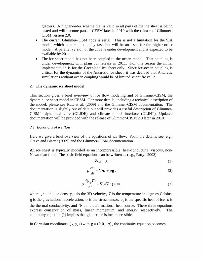
2. The dynamic ice sheet model

This section gives a brief overview of ice flow modeling and of Glimmer-CISM, the

dynamic ice sheet model in CESM. For more details, including a technical description of

the model, please see Rutt et al. (2009) and the Glimmer-CISM documentation. The

documentation is slightly out of date but still provides a useful description of Glimmer-

CISM’s dynamical core (GLIDE) and climate model interface (GLINT). Updated

documentation will be provided with the release of Glimmer-CISM 2.0 later in 2010.

2.1. Equations of ice flow

Here we give a brief overview of the equations of ice flow. For more details, see, e.g.,

Greve and Blatter (2009) and the Glimmer-CISM documentation.

An ice sheet is typically modeled as an incompressible, heat-conducting, viscous, non-

Newtonian fluid. The basic field equations can be written as (e.g., Pattyn 2003)

0=ui , (1)

d

dt= +

ugi , (2)

d(cpT )

dt= (k T ) + , (3)

where is the ice density, u is the 3D velocity, T is the temperature in degrees Celsius,

g is the gravitational acceleration, is the stress tensor, pc is the specific heat of ice, k is

the thermal conductivity, and is the deformational heat source. These three equations

express conservation of mass, linear momentum, and energy, respectively. The

continuity equation (1) implies that glacier ice is incompressible.

In Cartesian coordinates ( , , )x y z with (0,0, )g=g , the continuity equation becomes

0u v w

x y z+ + = , (4)

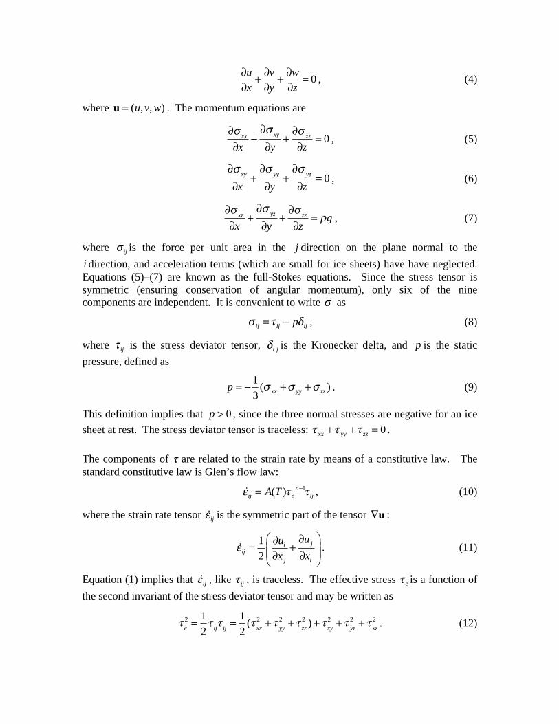
where ( , , )u v w=u . The momentum equations are

xx

x+

xy

y+

xz

z= 0 , (5)

xy

x+

yy

y+

yz

z= 0 , (6)

xz

x+

yz

y+

zz

z= g , (7)

where ij is the force per unit area in the j direction on the plane normal to the

i direction, and acceleration terms (which are small for ice sheets) have have neglected.

Equations (5)–(7) are known as the full-Stokes equations. Since the stress tensor is

symmetric (ensuring conservation of angular momentum), only six of the nine

components are independent. It is convenient to write as

ij ij ijp= , (8)

where ij is the stress deviator tensor, i j is the Kronecker delta, and p is the static

pressure, defined as

1

( )3

xx yy zzp = + + . (9)

This definition implies that 0p > , since the three normal stresses are negative for an ice

sheet at rest. The stress deviator tensor is traceless: 0xx yy zz+ + = .

The components of are related to the strain rate by means of a constitutive law. The

standard constitutive law is Glen’s flow law:

1( ) n

ij e ijA T= , (10)

where the strain rate tensor ij is the symmetric part of the tensor u :

1

2

jiij

j i

uu

x x= + . (11)

Equation (1) implies that ij , like ij , is traceless. The effective stress e is a function of

the second invariant of the stress deviator tensor and may be written as

e

2=

1

2 ij ij=

1

2(

xx

2+

yy

2+

zz

2 ) +xy

2+

yz

2+

xz

2 . (12)

The exponent is (10) is usually chosen as 3n = . The rate factor ( )A T is typically

computed using an Arrhenius relation (Payne et al. 2000):

*

*( ) exp

QA T a

RT= , (13)

where a is a proportionality constant, Q is the activation energy for creep, R is the

universal gas constant, *

0pmT T T T= + is the absolute temperature relative to the

pressure melting point pmT , and 0 273.15T = K is the triple point of water. Often it is

desirable to express the deviatoric stress in terms of the strain rate. Using the relation n

e eA= , equation (10) can be inverted to give

(1/ 1)( )e

n

ij ijB T= , (14)

where 1/ nB A= . This expression is of the standard form for a viscous fluid,

2ij ijμ= , (15)

where (1/ 1)( )e

nB Tμ = is the effective viscosity.

Using (8)–(14), the full-Stokes equations (5)–(7) together with the continuity equation (4)

can be written as a system of four coupled equations with four unknowns: u, v, w, and p.

Since these equations are hard to solve, most numerical ice sheet models solve the

momentum equation in approximate form. For example, Pattyn (2003) neglects the first

two terms on the LHS of (7) and uses a hydrostatic approximation,

zz

zg , (16)

to eliminate zz . After some algebraic manipulation, the resulting momentum equations

are

x(2

xx+

yy) +

xy

y+

xz

z= g

s

x, (17)

xy

x+

y(

xx+ 2

yy) +

yz

z= g

s

y, (18)

where s is the surface elevation. This is a set of two coupled equations in two

unknowns, u and v, which are easier to solve than the full-Stokes equations. Once u and

v are determined, w and p are found using the continuity equation (given that w = 0 at the

lower boundary) and the hydrostatic relation.

Equations (17)–(18) are often referred to as a “higher-order” approximation of the full-

Stokes equations. Other higher-order approximations exist; for example, Schoof and

Hindmarsh (2010) used an additional simplification to obtain a vertically averaged

higher-order model. In this model, u and v are solved in a single layer (rather than three

dimensions as in the Pattyn model), and the velocities at other elevations are found by

vertical integration.

Two lower-order approximations are widely used. The most common is the so-called

shallow-ice approximation (SIA), in which lateral and longitudinal stresses (the first two

terms on the LHS of (17) and (18)) are neglected. The SIA is valid in the slow-moving

interior of ice sheets, where basal sliding is small and the motion is dominated by vertical

shear. Another is the shallow-shelf approximation (SSA), in which vertical shear stresses

(the third terms on the LHS of (17) and (18)) are ignored. The SSA is valid for floating

ice shelves, where the basal shear stress is negligible and there is little or no vertical

shear. The SSA is sometimes used in modified form to model flow in regions of rapid

sliding, such as ice streams, where the basal shear stress is small but nonzero (e.g.,

MacAyeal 1989).

2.2. Glimmer, the Community Ice Sheet Model

Glimmer-CISM is a thermomechanical ice sheet model that solves the equations of ice

flow, given suitable approximations and boundary conditions. The source code is written

primarily in Fortran 90 and 95. The model resides on the BerliOS repository

(http://glimmer-cism.berlios.de/), where it is under active development. Glimmer-CISM

is an open-source code governed by the GNU General Public License and is freely

available to all.

The initial release of CESM contains source code from Glimmer-CISM version 1.6. The

main differences from version 1.0 are that (1) the directory structure has been

reorganized, and (2) the GLINT climate model interface has been significantly changed

to support coupling to CESM and other GCMs.

The dynamical core of the model, known as GLIDE, solves equations (1)–(3) for the

conservation of momentum, mass, and internal energy. The version of GLIDE currently

in CESM uses the shallow-ice approximation. However, a higher-order model is under

development and will be included in future releases.

The surface boundary conditions (e.g., the surface temperature and surface mass balance)

are supplied by a climate driver. When Glimmer-CISM is run in CESM, the climate

driver is GLINT, which receives the temperature and SMB from the coupler and

downscales them to the ice-sheet grid. The lower boundary conditions are given by an

isostasy model, which computes the elevation of the lower surface, and by a geothermal

model, which supplies heat fluxes at the lower boundary.

The model currently has simple treatments of basal hydrology and sliding. More

complex schemes for subglacial water hydrology and evolution of basal till strength are

under development. Glimmer-CISM also provides several simple schemes for calving at

the margins; these will be replaced by more realistic lateral boundary conditions in the

future.

For a detailed description of Glimmer-CISM’s dynamical core and software design,

please see Rutt et al. (2009) and the latest model documentation.

2.3. Directory structure

In the CESM directory structure, each model component sits under a directory with a

three-letter acronym: e.g., atm for the atmosphere model, lnd for the land surface, ocn for

the ocean, and ice for sea ice. The ice sheet component resides in a directory called glc.

Within the glc directory are three subdirectories: sglc (a stub model), xglc (a “dead”

model), and cism (the physical model).

Inside the cism subdirectory are several more subdirectories:

• source_glimmer_cism, which contains source code from Glimmer-CISM. Most

modules begin with the prefix “glide” (for GLIDE modules), “glint” (for GLINT

modules), or “glimmer” (for general-purpose modules).

• source_glc, which contains wrapper modules that link Glimmer-CISM to the

CESM coupler.

• source_slap, which has source code for the SLAP (Sparse Linear Algebra

Package) solvers used by Glimmer-CISM to solve implicit equations

• drivers, which contains two versions of the glc driver: one for use in the MCT

coupling framework and the other for the ESMF framework. The ESMF driver is

currently a placeholder.

• bld, which contains files required to build the code and create namelist files

• input_templates, which has config files for simulating the Greenland ice sheet at

various grid resolutions. Resolutions of 20 km, 10 km, and 5 km are currently

supported.

• tools, which contains tools for generating land/ice-sheet grid overlap files

• doc, which contains model documentation

• mpi and serial, which have appropriate versions of source code that can be used

for parallel and serial runs, respectively. Currently, only serial runs are

supported, and the only module used is glc_communicate.F90.

The code of most interest to users lies in the source_glimmer_cism, source_glc, and

input_templates directories. To change parameters in the config files that are read by

Glimmer-CISM at runtime, users should edit the appropriate file in input_templates. If

the file is edited before configuring the model, then the case directory will contain a

namelist script that will build a namelist with the desired parameters. Once the model has

been configured, runtime parameters can be changed by editing the namelist scripts

themselves.

The safest way to change source code in the source_glimmer_cism and source_glc

directories is to copy the file to the SourceMods/src.cism subdirectory within the case

directory and edit the file there. When the code is built, the contents of src.cism will

automatically overwrite any files of the same name in the model source code directories.

2.4. Coupling to CLM

GLINT, the climate model interface of Glimmer-CISM, is designed to accumulate,

average, and downscale fields received from other climate model components. These

fields are interpolated from a global grid to the individual ice sheet grid(s). In general

there can be multiple non-overlapping ice sheet grids, but only Greenland is currently

enabled. The global grid must be a regular lat-lon grid, but the latitudes need not be

equally spaced. For CESM the global grid is assumed to be the same as the CLM grid.

GLINT needs to know (1) one or more 2D fields necessary for computing the surface

mass balance, (2) an upper boundary condition, usually surface temperature, and (3) the

latitudes and longitudes of the grid cells where these fields are defined. There are two

general ways of computing the surface mass balance:

1. a positive-degree-day (PDD) scheme, either annual or daily, for which the

required inputs to GLINT are the 2m air temperature and the precipitation. This

is the default scheme for Glimmer-CISM, but it may not be appropriate for

climate change studies. The PDD option is not currently enabled for CESM runs,

but will soon be added as an option for comparison with the surface-mass-balance

scheme.

2. a surface-mass-balance (SMB) scheme for land ice embedded in CLM. In this

case the required input to GLINT is the SMB itself. This is the preferred strategy

for climate experiments. The mass balance is computed for a specified number of

elevation classes for each cell on the coarser land grid (~100 km). This is much

less computationally expensive than computing the SMB for each cell on the finer

ice sheet grid (~10 km). Values of 1, 3, 5, and 10 elevation classes are currently

supported, with 10 being the default.

For the SMB scheme, the fields passed to GLINT are (1) the surface mass balance, qsmb

(kg/m2/s, positive for ice growing, negative for ice melting), (2) the surface temperature,

Tsfc (deg C), and (3) the surface elevation, topo (m) for each elevation class.

These fields are received from the coupler once per simulation day, accumulated and

averaged over the course of a mass balance accumulation time step (typically one year)

and then are downscaled to the ice sheet grid. The downscaling occurs in two phases.

First, the values on the global grid are interpolated in the horizontal to the local ice sheet

grid. Next, for each local grid cell, values are linearly interpolated between adjacent

elevation classes. For example, suppose that at a given location the coupler supplies a

surface mass balance at elevations of 300 and 500 m, whereas the local gridcell has an

elevation of 400 m. Then the local SMB is computed to be equal to the average of the

SMB at 300 and 500 m.

In some parts of the ice sheet grid the fields supplied by CLM are not valid, simply

because there are no land-covered global gridcells in the vicinity. For this reason,

GLINT computes a mask on the global grid at initialization. The mask has a value of 1

for global gridcells that have a nonzero land fraction (and hence supply valid data) and is

zero otherwise. GLINT then computes a local mask for each gridcell on the ice sheet

grid. The local mask has a value of 1 if one or more of the four nearest global neighbors

supplies valid data (i.e., has a global mask of 1). Otherwise, the local mask has a value of

zero. In this case ice sheets are not allowed to exist, and in output files, the SMB and

temperature fields are given arbitrary values, typically zero. This masking has not yet

proved to be a restriction in practice, since the Greenland ice sheet does not extend far

from the land margin. Alternatives may need to be considered for modeling the Antarctic

ice sheet.

After downscaling the surface mass balance to the ice sheet grid, GLINT calls the ice

sheet dynamics model, which returns a new profile of ice sheet area and extent. The

following fields can be upscaled to the global grid and returned from GLINT to the

coupler: (1) the ice area fraction, gfrac, (2) the ice sheet elevation, gtopo (m), (3), the

frozen portion of the freshwater runoff, grofi, (4) the liquid portion of the runoff, grofl,

and (5) the heat flux from the ice sheet interior to the surface, ghflx. These fields are

computed for each elevation class of each grid cell. The frozen runoff corresponds to

iceberg calving and the liquid runoff to basal meltwater. Surface runoff is not supplied

by GLINT because it has already been computed in CLM. Upscaling is not enabled in

the current release but will be included in the near future.

There are two modes of coupling Glimmer-CISM to CLM: one-way and two-way. For

one-way coupling, Glimmer-CISM receives the surface mass balance from CLM via the

coupler, and the ice sheet extent and thickness evolve accordingly. However, the land

surface topography is fixed, and the fields received by CLM from the ice sheet model are

ignored. In this case CLM computes surface runoff as in earlier versions of CCSM:

Excess snow is assumed to run off, and melted ice stays put at the surface. (See Section 3

for more details.) For two-way coupling, the CLM surface topography is modified based

on input from the ice sheet model. In this case, surface runoff is computed in a more

realistic way; excess snow remains in place and is converted to ice, and melted ice runs

off. In either case, CLM computes the surface runoff, which is directed toward the ocean

by the river routing scheme. Only one-way coupling is currently enabled, but two-way

coupling is under development and will be added later in 2010.

2.5. Configuring and running the model

Timesteps: There are several kinds of timesteps in Glimmer-CISM.

1. The forcing timestep is the interval in hours between calls to GLINT. Currently,

the forcing timestep is the same as the coupling interval, which is 24 hours.

GLINT is called every time information is passed from the coupler to GLC, i.e.,

once per day.

2. The mass balance timestep is the interval over which accumulation/ablation

forcing data is summed and averaged. The current default is one year. This

means that GLINT will accumulate forcing data from the coupler over 365 daily

forcing timesteps and average the data before downscaling it to the local ice sheet

grid. The mass balance timestep must be an integer multiple of the forcing

timestep.

3. The ice sheet timestep is the interval in years between calls to the dynamic ice

sheet model, GLIDE. The ice sheet timestep must be an integer multiple of the

mass balance timestep.

Two optional runtime parameters can be used to make the time-stepping more intricate:

1. The mass balance accumulation time, mbal_accum_time (in years), is the period

over which mass balance information is accumulated before calling GLIDE. By

default, the mass balance accumulation time is equal to the ice sheet timestep.

But suppose, for example, that the ice sheet timestep is 5 years. If we set

mbal_accum_time = 1.0, we accumulate mass balance information for 1 year and

use this mass balance to force the ice sheet model (thus avoiding 4 additional

years of accumulating mass balance data).

2. The timestep multiplier, ice_tstep_multiply, is equal to the number of ice sheet

timesteps executed for each accumulated mass balance field. Suppose that the

mass balance timestep is 1 year, the ice sheet timestep is 1 year, and

ice_tstep_multiply = 10. GLINT will accumulate and average mass balance

information for 1 year, then execute 10 ice sheet model timesteps of 1 year each.

In other words, the ice sheet dynamics is accelerated relative to the land and

atmosphere. This option is likely to be useful in CESM for multi-millennial ice-

sheet simulations where it is impractical to run the atmosphere and ocean models

for more than a few centuries.

These various options are set in the ice configuration file (e.g., ice.config.gland20) in the

input_templates directory. This file contains (or may contain) the following timestep

information:

1. The ice sheet timestep dt (in years) is set in the section [time] in the ice config

file.

2. The mass balance time step is not set directly in the config file, but is related to

the accumulation/ablation mode, acabmode, which is set in the section [GLINT

climate]. If acabmode = 1 (the default value for CESM runs), then the mass

balance time step is set to the number of hours in a year (i.e., 8760 hours for a

365-day year).

3. The values of ice_tstep_multiply and mbal_accum_time, if present, are listed in

the section [GLINT climate].

See the Glimmer-CISM documentation for more details.

Note that the total length of the simulation is not determined by Glimmer-CISM, but is

set in the file env_run.xml in the case directory.

Input/output: All model I/O is in netCDF format. Near the end of the config file, there

are sections labeled [CF input] and [CF output]. The CF input section contains the name

of the ice sheet grid file used for initialization. This file typically includes the ice

thickness and surface elevation, or equivalent information, in each grid cell. Other

information (e.g., internal ice temperature) may be included; if not, then these fields are

set internally by Glimmer-CISM.

The CF output section determines the names of the various output files, the variables to

be written to each file, and the frequency with which files are written. The defaults are to

write output to a history file (suffix ‘h’) and a restart file (suffix ‘hot’, denoting a

Glimmer-CISM hotstart file) once a year. Among the standard fields written to the

history file are the ice thickness (thk), upper surface elevation (usurf), temperature

(temp), and velocity (uvel, vvel) fields, along with the surface mass balance (acab) and

surface air temperature (artm) downscaled to the ice sheet grid.

The restart or hotstart file contains all the fields required for exact restart. However, the

restart will be exact only if the file is written immediately after an ice dynamics time step.

This will normally be the case for restart files written at the end of any model year.

Many other fields can be written out if desired, simply by adding them to variable list in

the config file. The source files with names “*_io.F90” specify the fields than can be

written out. The easiest way to write out new variables is to add them to a file ending in

“vars.def” and then rebuild the “*_io.F90” files using a python script. These files and

scripts are not part of the standard CESM release but can be obtained by checking out

Glimmer-CISM from the BerliOS repository.

Grids: GLINT can downscale fields from any global lat/lon grid. The latitude lines need

not be equally spaced. Three global grid resolutions are currently supported: T31

(spectral), FV2 (~2o finite-volume), and FV1 (~1

o finite-volume). The global resolution

(i.e., the resolution of the land and atmosphere) is set when a case is created.

Local ice sheet grids must be rectangular; typically they are polar stereographic

projections. For Greenland, three grids are currently supported, with resolutions of 20

km, 10 km, and 5 km, respectively. The current default is 20 km. This can be changed

by modifying GLC_GRID to the desired value (e.g., gland10 or gland5) in env_conf.xml

before configuring the case. When the model is configured, config files values are taken

automatically from the appropriate file (e.g., ice.config.gland10 for 10-km resolution) in

input_templates. Each local grid is compatible with any of the three supported global

resolutions.

Simulating the Greenland Ice Sheet: A primary motivation for having a CESM ice

sheet model is to do climate change experiments with a dynamic Greenland Ice Sheet

(GrIS). The first step is to simulate a present-day (or preindustrial) ice sheet that is in

steady-state with the CESM climate and is not too different in thickness, extent, and

velocity from the real GrIS. If we cannot do this, then either we will start climate change

simulations with an unrealistic GrIS, or we will start with a realistic GrIS that is far from

steady state, making it difficult to distinguish the climate-change signal from model

transients.

It may be challenging to generate a realistic ice sheet, for several reasons: (1) The

surface mass balance computed in CESM could be inaccurate; (2) Glimmer-CISM

currently uses the shallow-ice approximation, which is not accurate for fast outlet

glaciers; and (3) the present-day GrIS may not be in steady-state with the present-day (or

preindustrial) climate. Our working hypotheses are that (1) If the SMB is reasonably

accurate, we can obtain a reasonable large-scale thickness and extent for the GIS; (2)

With a higher-order dynamics scheme and some judicious tuning, we can generate ice

streams and outlet glaciers in the right locations with realistic velocities; and (3) The

present-day GrIS is not far from steady-state with the preindustrial climate. These

hypotheses are now being tested; results will be reported in an upcoming special issue of

the Journal of Climate.

Obtaining an accurate surface mass balance may require some tuning in CLM; see

Section 3 for details. We are also experimenting with different dynamics settings in the

ice config file. The current default settings may not be optimal. The config files will be

updated when we have more experience in running the model.

3. Ice sheets in the Community Land Model

This section describes changes made in CLM4 to accommodate ice sheets. For more

information, see the CLM4 documentation.

3.1. CLM and the surface mass balance of ice sheets

The surface mass balance of a glacier or ice sheet is the net annual accumulation/ablation

of mass at the upper surface. Ablation is defined as the mass of water that runs off to the

ocean. Not all the surface meltwater runs off; some of the melt percolates into the snow

and refreezes. Accumulation is primarily by snowfall and deposition, and ablation is

primarily by melting and evaporation/sublimation.

Two kinds of surface mass balance schemes are widely used in ice sheet models:

• positive-degree-day (PDD) schemes, in which the melting is parameterized as a

linear function of the number of degree-days above the freezing temperature. The

proportionality factor is empirical and is larger for bare ice than for snow.

• surface energy-balance (SEB) schemes, in which the melting depends on the sum

of the radiative, turbulent, and conductive fluxes reaching the surface.

The current version of Glimmer-CISM has only a PDD scheme. It is generally believed

that PDD schemes are not appropriate for climate change studies, because empirical

degree-day factors could change in a warming climate. Comparisons of PDD and energy-

balance schemes (e.g., van de Wal 1996; Bougamont et al. 2007) suggest that PDD

schemes may be overly sensitive to warming temperatures. Bougamont et al. (2007)

found that a PDD scheme generates runoff rates nearly twice as large as those computed

by an SEB scheme.

In CESM, the ice sheet surface mass balance is computed using an SEB scheme in CLM.

Before discussing the scheme, it is useful to describe CLM’s hierarchical data structure.

Each gridcell is divided into one or more landunits; landunits can be further divided into

columns; and columns can be subdivided into plant functional types, or PFTs. Each

column within a landunit is characterized by a distinct snow/soil or snow/ice temperature

and water profile. PFTs within a column have the same vertical profiles but can have

different surface fluxes. In the current version, landunit areas in each gridcell are fixed at

initialization, but PFT and column areas can evolve during the simulation.

Previously, CLM supported up to five landunits per grid cell: soil, urban, wetland, lake,

and glacier landunits. Each of these landunits generally contains a single column, and

soil columns (but not urban, wetland, lake, and glacier columns) consist of multiple

PFTs. The ice-sheet-friendly version of CLM supports a sixth landunit, glacier_mec,

where “mec” denotes “multiple elevation classes”. Each glacier_mec landunit is divided

into a user-defined set of columns based on surface elevation. The default is 10 elevation

classes whose lower boundaries are 0, 200, 400, 700, 1000, 1300, 1600, 2000, 2500, and

3000 m. Each column is characterized by a fractional area and surface elevation that are

read in during model initialization. The fractional area and elevation in each column are

allowed to evolve during the run. Each glacier_mec column within a grid cell has distinct

ice and snow temperatures, snow water content, surface fluxes, and surface mass balance.

These elevation classes provide a mechanism for downscaling the surface mass balance

from the relatively coarse (~100 km) land grid to the finer (~10 km) ice sheet grid. The

SMB is computed for each elevation class in each grid cell and is accumulated, averaged,

and passed to the GLC (dynamic ice-sheet) component via the coupler once per day. The

mass balance is downscaled by GLINT to the ice-sheet grid as described in Section 2

above.

There are several reasons for computing the surface mass balance in CLM rather than in

Glimmer-CISM:

1. It is much cheaper to compute the SMB in CLM for ~10 elevation classes than in

Glimmer-CISM. For example, suppose we are running CLM at a resolution of

~50 km and Glimmer at ~5 km. Greenland has dimensions of about 1000 x 2000

km. For CLM we would have 20 x 40 x 10 = 8,000 columns, whereas for

GLIMMER we would have 200 x 400 = 80,000 columns.

2. We take advantage of the sophisticated snow physics parameterization already in

CLM instead of implementing a separate scheme for Glimmer-CISM. When the

CLM scheme is improved, the improvements are applied to ice sheets

automatically.

3. The atmosphere model can respond during runtime to ice-sheet surface changes.

As shown by Pritchard et al. (2008), runtime albedo feedback from the ice sheet is

critical for simulating ice-sheet retreat on paleoclimate time scales. Without this

feedback, the atmosphere warms much less, and the retreat is delayed.

4. Mass is conserved, in that the rate of surface ice growth or melting computed in

CLM is equal to the rate seen by the dynamic ice sheet model.

5. The improved surface mass balance is available in CLM for all glaciated grid

cells (e.g., in the Alps, Rockies, Andes, and Himalayas), not just those which are

part of ice sheets.

3.2. Details of the surface-mass-balance and coupling schemes

When the model is initialized, CLM reads a high-resolution data file classifying each

point as soil, urban, lake, wetland, glacier, or glacier_mec. For runs with dynamic ice

sheets, the default is to classify all glaciated regions as glacier_mec. If there are no

dynamic ice sheets, then these regions are normally classified as glacier landunits with a

single column per landunit. Glacier_mec columns, like glacier columns, are initialized

with a temperature of 250 K. While glacier columns are initialized with a snow liquid

water equivalent (LWE) equal to the maximum allowed value of 1 m, glacier_mec

columns begin with a snow LWE of 0.5 m so that they will reach their equilibrium mean

snow depth sooner.

Surface fluxes and the vertical temperature profile are computed independently for each

glacier_mec column. Each column consists of 15 ice layers and up to 5 snow layers,

depending on snow thickness. As for other landunits with a snow cover, surface albedos

are computed based on snow fraction, snow depth, snow age, and solar zenith angle. The

bare ice albedo is prescribed to be 0.50 by default; this is lower than the values assumed

by CLM for glacier landunits (0.80 for visible radiation and 0.55 for near IR). The latter

values are higher than those usually assumed by glaciologists.

The atmospheric surface temperature, potential temperature, specific humidity, density,

and pressure are downscaled from the mean gridcell elevation to the glacier_mec column

elevation using a specified lapse rate (typically 6.0 deg/km) and an assumption of

uniform relative humidity. At a given time, lower-elevation columns can undergo surface

melting while columns at higher elevations remain frozen. This results in a more accurate

simulation of summer melting, which is a highly nonlinear function of air temperature.

The precipitation rate and radiative fluxes are not currently downscaled, but could be in

the future if care were taken to preserve the cell-integrated values.

CLM has a somewhat unrealistic treatment of accumulation and melting on glacier

landunits. The snow depth is limited to a prescribed depth of 1 m liquid water equivalent,

with any additional snow assumed to run off to the ocean. (This amounts to a crude

parameterization of iceberg calving.) Snow melting is treated in a realistic fashion, with

meltwater percolating downward through snow layers as long as the snow is unsaturated.

Once the underlying snow is saturated, any additional meltwater runs off. When glacier

ice melts, however, the meltwater is assumed to remain in place until it refreezes. In

warm parts of the ice sheet, the meltwater does not refreeze, but stays in place

indefinitely.

In the modified CLM with glacier_mec columns, snow in excess of the prescribed

maximum depth is converted to ice, contributing a positive surface mass balance to the

ice sheet model. When ice melts, the meltwater is assumed to run off to the ocean,

contributing a negative surface mass balance. The net SMB associated with ice formation

(by conversion from snow) and melting/runoff is computed for each column, averaged

over the coupling interval, and sent to the coupler. This quantity, denoted qice, is then

passed to GLINT, along with the surface elevation topo in each column. GLINT

downscales the SMB (renamed as qsmb) to the local elevation on the ice sheet grid,

interpolating between values in adjacent elevation classes. The units of qice are mm/s, or

equivalently km/m2/s. If desired, the downscaled quantities can be multiplied by a

normalization factor to conserve mass exactly. (This normalization is not yet

implemented.)

Note that the surface mass balance typically is defined as the total accumulation of ice

and snow, minus the total ablation. The qice flux passed to GLINT is the mass balance

for ice alone, not snow. We can think of CLM as owning the snow, whereas Glimmer

owns the underlying ice. The snow depth can fluctuate between 0 and 1 m LWE without

Glimmer-CISM knowing about it.

In addition to qice and topo, the ground surface temperature tsfc is passed from CLM to

GLINT via the coupler. This temperature serves as the upper boundary condition for

Glimmer-CISM’s temperature calculation.

Given the SMB from the land model, Glimmer-CISM executes one or more dynamic

time steps and then has the option to upscale the new ice sheet geometry to the global

grid and return it to CLM via the coupler. The fields passed to the coupler for each

elevation class are the ice sheet fractional area (gfrac), urface elevation (gtopo), liquid

(basal meltwater) runoff grofl, frozen (calving) runoff grofi, and surface conductive heat

flux ghflx.

The current coupling is one-way only. That is, CLM sends the SMB and surface

temperature to GLINT but does not do anything with the fields that are returned. Thus the

CLM surface topography is fixed in time. This is permissible for century-scale runs in

which ice-sheet elevation changes are modest. For longer runs with larger elevation

changes, two-way coupling is highly desirable. A two-way coupling scheme is under

development.

3.3. Model controls

The number of elevation classes is glc_nec, an integer declared in module

clm_varctl.F90. This number is set equal to the value specified for GLC_NEC in the file

env_build.nml in the case directory. Values of 1, 3, 5, and 10 elevation classes are

currently supported, with 10 classes being the default. The number of classes cannot

exceed maxpatch_glcmec, an integer parameter set in clm_varpar.F90. Currently,

maxpatch_glcmec = 10.

The array glc_topomax, which is set in subroutine clmvarctl_init, defines the maximum

elevation (in meters) in each class. For 10 elevation classes, glc_topomax is set to (0,

200, 400, 700, 1000, 1300, 1600, 2000, 2500, 3000, 10000).

At initialization, CLM reads a data file specifying the areal percentage of each grid cell

classified as wetland, vegetation, lake, urban, glacier, or glacier_mec. For glacier_mec

cells, the area and surface elevation are specified in each elevation classes. The area and

surface elevation in each elevation class may change during the course of the run, but the

total glacier_mec area in a given gridcell is fixed; glacier_mec landunits cannot change to

vegetated landunits or vice versa. This restriction will be relaxed in future model

releases.

The fundamental control variable is create_glacier_mec_landunit, a logical variable that

is declared in clm_varctl.F90. It is false by default, but is automatically set to true when

we create a case that includes a dynamic ice sheet component (e.g., IG, FG, or BG). If

create_glacier_mec_landunit = T, the following occurs:

• The array glc_topomax is defined appropriately based on glc_nec.

• Memory is allocated for the areal percentage (pct_glcmec) and surface elevation

(topo_glcmec) in each elevation class, and these values are read in from a

netCDF file. The sum of pct_glcmec in each grid cell is checked to make sure it

agrees with pctgla, the total glaciated fraction in each gridcell.

• Glacier_mec landunits and columns are defined for all gridcells where either (1)

the fractional glacier area is greater than zero or (2) the dynamic ice sheet model

may require a surface mass balance, even if CLM does not have glacier landunits

in that location. To allow for case (2), grid overlap files have been precomputed.

For given resolutions of CLM and Glimmer-CISM, these files identify all CLM

cells that have nonzero ice area and overlap with any part of the ice sheet grid. In

these overlapping cells, glacier_mec columns are defined in all elevation classes.

Columns with zero area are known as “virtual” columns. These columns do not

affect energy exchange between the land and the atmosphere, but are included for

potential forcing of Glimmer-CISM.

The logical variable glc_smb determines what kind of information is passed from CLM to

the ice sheet model via the coupler. If glc_smb is true, then the surface mass balance is

passed. Specifically, qice is interpreted by the ice sheet model as a flux (kg/m2/s) of ice

freezing/melting. If glc_smb is false, then the ice sheet model should compute the

surface mass balance using a positive-degree-day scheme, with qice interpreted as the

precipitation and tsfc as the 2-m air temperature. (The PDD option is not currently

supported, but will be included in a future release.) In either case, tsfc is downscaled and

applied as the upper boundary condition for the dynamic ice sheet.

The logical variable glc_dyntopo controls whether CLM surface topography changes

dynamically as the ice sheet evolves (i.e., whether the coupling is one-way or two-way).

The default (and the only option currently supported) is glc_dyntopo = F, in which case

the land topography is fixed. In this case the surface runoff for glacier_mec landunits is

computed as for glacier landunits: (1) Any snow in excess of 1 m LWE runs off to the

ocean, and (2) Melted ice remains in place until it refreezes. Excess snow and melted ice

still contribute to positive and negative values, respectively, of qice, but only for the

purpose of forcing Glimmer-CISM.)

If glc_dyntopo = T, then CLM receives updated topographic information from the ice

sheet model. In this case the CLM surface runoff is computed in a more realistic way: (1)

Any snow in excess of 1 m LWE is assumed to turn to ice and does not run off. (2)

Melted ice runs off.

Two physical parameters may be useful for tuning the surface mass balance: (1) the

surface bare ice albedo, albice, which is set in SurfaceAlbedoMod.F90, and (2) the

surface air temperature lapse rate, lapse_glcmec, which is used for downscaling

temperature and is set in clm_varcon.F90. By default, the bare ice albedo is 0.80 for

visible wavelengths and 0.55 for near IR, but for glacier_mec columns the bare ice albedo

is automatically reduced to 0.50 in the namelist. The default lapse rate is 6.0 deg/km.

The snow albedo is not easily tunable. It is computed in a complicated way based on

snow fraction, snow depth, snow age, and solar zenith angle. Snow albedo in

glacier_mec columns is treated identically to snow in other landunits.

Another possible tuning mechanism is to convert rain to snow and vice versa as a

function of surface temperature. This conversion would violate conservation of latent

heat, but might give more realistic precipitation fields in columns with elevations much

higher or lower than the grid-cell mean.

The default values of albice, create_glacier_mec_landunit, glc_smb, and glc_dyntopo

may each be overwritten by specifying the desired values in the namelist. This is done

automatically for albice and create_glacier_mec_landunit when a case is created with

dynamic ice sheets.

4. Future developments

This section lists model features that are planned or desirably but not yet implemented.

Many of these are mentioned in the text above, but are included here for reference. In

each section, future developments are listed roughly in order from easy, near-term

improvements to more extensive, long-term improvements.

4.1. Bug fixes

One major bug was identified after the code for the initial CESM release was frozen. The

config files for the 10-km and 5-km Glimmer-CISM grids (ice.config.gland10 and

ice.config.gland5) contain incorrect settings for the map projection. The sections labeled

[GLINT projection] should be deleted and replaced by the following:

[projection]

type = 'STERE'

centre_latitude = 90.0

centre_longitude = 321.0

false_easting = 800000.0

false_northing = 3400000.0

standard_parallel = 71.0

The existing 20-km config file is correct. The other two files will be fixed in the next code

release.

4.2. Glimmer-CISM

• Add ESMF capability. (Coupling currently is supported for MCT only.)

• Enable exact restart when restart files are written in mid-year (requires writing

some GLINT variables to restart files).

• Enable short (~5-day) tests that exercise GLIDE.

• Define elevation classes by reading CLM surface data files (to guarantee

consistency).

• Enable the PDD scheme for comparison to the surface mass balance received

from CLM.

• Upscale GLC CLM coupling fields (gfrac, gtopo, grofi, grofl, ghflx) correctly to

the global grid.

• Support creation of *_io.F0 files from *vars.def files with supported software

(i.e., an alternative to python scripts). Similarly for glimmer_vers file.

• Restructure the GLINT interface, reducing the number of extraneous arguments.

• Modify Greenland configuration files to optimize agreement with present-day

thickness and extent.

• Upgrade to Glimmer-CISM 2.0 (serial version) with higher-order dynamics and

Trilinos solver capabilities.

• Develop a suitable Greenland initial condition for higher-order simulations.

• Upgrade to a parallel version of Glimmer-CISM.

• Implement coupling to the POP ocean model.

4.3. CLM

• Add a switch for making frain/fsnow dependent on surface temperature.

• For glacier_mec landunits, specify distinct bare ice albedos for visible and near

IR.

• Add diagnostics to track mass balance terms (e.g., total runoff, refreezing, and

total melt).

• Add some daily diagnostics (e.g., for melting and albedo).

• Evaluate sensitivity to maximum snowpack depth; perhaps increase to > 1 m.

• Develop a modified surface data file with ice-free gridcells near northern margin

(in agreement with other ice-sheet datasets)

• Develop data sets to force CLM with output from other GCMs.

• Enable two-way coupling of CLM and Glimmer-CISM.

• Implement parameterization for area and volume evolution of glaciers and ice

caps.

5. Acknowledgments

Many researchers in the glaciology and climate modeling communities have contributed

to this work. Miren Vizcaíno (UC Berkeley) has worked closely on the development of

the surface-mass-balance scheme and analysis of model output. Jon Wolfe (NCAR) is

the lead software engineer for the project; his efforts have been critical in integrating the

new ice sheet component in CESM. Tony Craig, Erik Kluzek, David Lawrence, and

Mariana Vertenstein (NCAR) have supported with overall software development,

including the incorporation of ice sheets in CLM.

Development of Glimmer-CISM is overseen by a steering committee consisting of

Magnus Hagdorn (U. Edinburgh), Jesse Johnson (U. Montana), William Lipscomb

(LANL), Tony Payne (U. Bristol), Stephen Price (LANL), and Ian Rutt (U. Swansea).

They and many others have contributed to the dynamic ice sheet model.

Anjuli Bamzai (formerly DOE, now NSF), Jay Fein (NSF), Renu Joseph (DOE), and

Julie Palais (NSF) have provided essential funding ice sheet model development and

integration into CESM. Phil Jones (LANL) has supported this work as manager of

LANL’s COSIM project and as co-PI, with John Drake (ORNL), of the DOE SciDAC

project that has funded much of this effort.

Lali Chatterjee and William Spotz (DOE) have directed the DOE Ice Sheet Initiative for

Climate ExtremeS (ISICLES) project, which is contributing to numerical advances that

are now being incorporated in Glimmer-CISM. William Collins (LBNL) has led the

Investigation of the Magnitudes and Probabilities of Abrupt Climate TransitionS

(IMPACTS) project, which is developing new ice-ocean coupling methods that will be

incorporated in future versions of CESM.

William Collins, Peter Gent and James Hurrell have supported this project while

managing overall CCSM/CESM development at NCAR. David Holland (NYU), Jeff

Ridley (U.K. Met Office), Slawek Tulaczyk (UC Santa Cruz), and many others have

given helpful advice and encouragement along the way.

6. References

Bougamont, M., Bamber, J.L., Ridley, J.K., Gladstone, R.M., Greuell, W., Hanna, E.,

Payne, A.J. and Rutt, I., 2007: Impact of model physics on estimating the surface

mass balance of the Greenland ice sheet. Geophysical Research Letters 34:

10.1029/2007GL030700.

Cazenave, A., K. Dominh, S. Guinehut, E. Berthier, W. Llovel, G. Ramilien, M. Ablain,

and G. Larnicol, 2008: Sea level budget over 2003-2008: A reevaluation from

GRACE space gravimetry, satellite altimetry, and Argo, Global and Planetary

Change, doi:10.1016/j.gloplacha.2008.10.004.

Greve, R., and H. Blatter, 2009: Dynamics of Ice Sheets and Glaciers. Springer, Berlin,

287 pp.

Holland, D.M., R.H. Thomas, B. De Young, M.H. Ribergaard, B. Lyberth, 2008a:

Acceleration of Jakobshavn Isbrae triggered by warm subsurface ocean waters.

Nature Geo., 1, 659-664.

Holland, P.R., Jenkins, A., and D.M. Holland, 2008b, The response of ice shelf basal

melting to variations in ocean temperature, Journal of Climate, 21, 2558-2572.

Lipscomb, W., R. Bindschadler, E. Bueler, D. Holland, J. Johnson, and S. Price, 2009: A

community ice sheet model for sea-level prediction, Eos Trans. AGU, 90, 23.

Little, C. M., M. Oppenheimer, R. B. Alley, V. Balaji, G. K. C. Clarke, T. L. Delworth,

R. Hallberg, D. M. Holland, C. L. Hulbe, S. Jacobs, J. V. Johnson, H. Levy, W. H.

Lipscomb, S. J. Marshall, B. R. Parizek, A. J. Payne, G. A. Schmidt, R. J. Stouffer, D.

G. Vaughan, and M. Winton, 2007: Toward a new generation of ice sheet models,

Eos Trans. AGU, 88, 578-579, doi:10.1029/2007EO520002.

MacAyeal, D.R., 1989: Large-scale ice flow over a viscous basal sediment: Theory and

application to Ice Stream B, Antarctica, J. Geophys. Res., 94 (B4), 4071-4087.

Meehl, G. A., et al., 2007: Global climate projections, in Climate Change 2007:

Contribution of Working Group I to the Fourth Assessment Report of the IPCC,

edited by S. Solomon et al., pp. 747–846, Cambridge Univ. Press, New York.

Meier, M.F., Dyurgerov, M.B., Rick, U.K., O’Neel, S., Pfeffer, W.T., Anderson, R.S.,

Anderson, S.P., and Glazovsky, A.F., 2007: Glaciers dominate eustatic sea-level rise

in the 21st century, Science, 317, 1064-1067.

Pattyn, F., 2003: A new three-dimensional higher-order thermomechanical ice sheet

model: Basic sensitivity, ice stream development, and ice flow across subglacial

lakes, J. Geophys. Res., 108(B8), 2382, doi:10.1029/2002JB002329.

Pritchard, M. S., A. B. G. Bush, and S. J. Marshall, 2008: Neglecting ice-atmosphere

interactions underestimates ice sheet melt in millennial-scale deglaciation

simulations. Geophys. Res. Lett. 35, L01503, doi:10.1029/2007GL031738.

Radi , V., and Hock, R., 2010, Regional and global volumes of glaciers derived from

statistical upscaling of glacier inventory data, J. Geophys. Res., 2215, F01010.

Rahmstorf, S., 2007: A semi-empirical approach to projecting future sea-level rise,

Science, 315, 368-370.

Rignot, E., Bamber, J.L., van den Broeke, M.R., Davis, C., Li, Y., van de Berg, W.J., and

van Meijgaard, E., 2008: Recent Antarctic ice mass loss from radar interferometry

and regional climate modeling, Nature Geosci., 1, 106-110.

Rutt, I., Hagdorn, M., Hulton, N.J.R., and Payne, A.J., 2009: The Glimmer community

ice sheet model, J. Geophys. Res., 114, F02004.

Schoof, C. and R.C.A. Hindmarsh, 2010: Thin-film flows with wall slip: An asymptotic

analysis of higher order glacier flow models, Quart. J. Mech. Appl. Math., 63, 73-

114; doi: 10.1093/qjmam/hbp025.

van de Wal, R.S.W., 1996: Mass-balance modeling of the Greenland ice sheet: A

comparison of an energy-balance and a degree-day model. Annals of Glaciology 23:

36-45.

van den Broeke, M., Bamber, J., Ettema, J., Rignot, E., Schrama, E., van der Berg, W.J.,

van Meijgaard, E., Velicogna, I., and B. Wouters, 2009: Partitioning recent Greenland

mass loss, Science, 326, 984-986.

Velicogna, I., 2009: Increasing rates of ice mass loss from the Greenland and Antarctic

ice sheets revealed by GRACE, Geophys. Res. Lett., 36, L19503.