Staff Papers Series

P91-38 September 1991

AGGREGATION OVER CONSUMERS AND THE

ESTIMATION OF A DEMAND SYSTEM FOR U.S. FOOD

Cesar Falconi

and

Ben Senauer

LIrf

Department of Agricultural and Applied Economics

University of MinnesotaInstitute of Agriculture, Forestry and Home Economics

St. Paul, Minnesota 55108

P91-38 September 1991

AGGREGATION OVER CONSUMERS AND THEESTIMATION OF A DEMAND SYSTEM FOR U.S. FOOD

Cesar Falconi

and

Ben Senauer*

*The authors are graduate research assistant and professor,respectively, in the Department of Agricultural and AppliedEconomics at the University of Minnesota.

The University of Minnesota is committed to the policy that allpersons shall have equal access to its programs, facilities, andemployment without regard to race, religion, sex, national origin,handicap, age, veteran status, or sexual orientation.

Staff Papers are published by the Department of Agricultural andApplied Economics without formal review.

AGGREGATION OVER CONSUMERS AND THEESTIMATION OF A DEMAND SYSTEM FOR U.S. FOOD

ABSTRACT

This paper estimates a complete demand system for foodfor the United States using an extension of the Almost IdealDemand System (AIDS) with household and aggregate data. Themajor purpose is to explore the implications of aggregationover consumers. Empirical evidence, based on data from the1980-87 Continuing Consumer Expenditure Surveys, shows thatthe regression results and demand elasticities of thehousehold and aggregate models and data can be very similar.Further results reveal factors which affect the similarity ofthe household and aggregate estimates.

I. INTRODUCTION

Most of the existing literature on the estimation of

complete demand systems is based on time-series data. These

studies provide price and income effects for all consumers or

households as a whole, but yield few implications concerning

the effect of relevant demographic characteristics on demand.

The degrees of freedom also are typically small. Moreover,

most time-series studies treat the data as if they relate to

a single consumer. As Deaton and Muellbauer (1980b) observe,

"if the data are available for only aggregates of households,

there are no obvious grounds why the theory, formulated for

individual households, should be directly applicable" (p.

148).

There are few studies in the literature on complete

demand systems which have utilized micro (household) data,

which is generated by cross-sectional or panel surveys.

Micro data make possible the estimation of disaggregate income

1

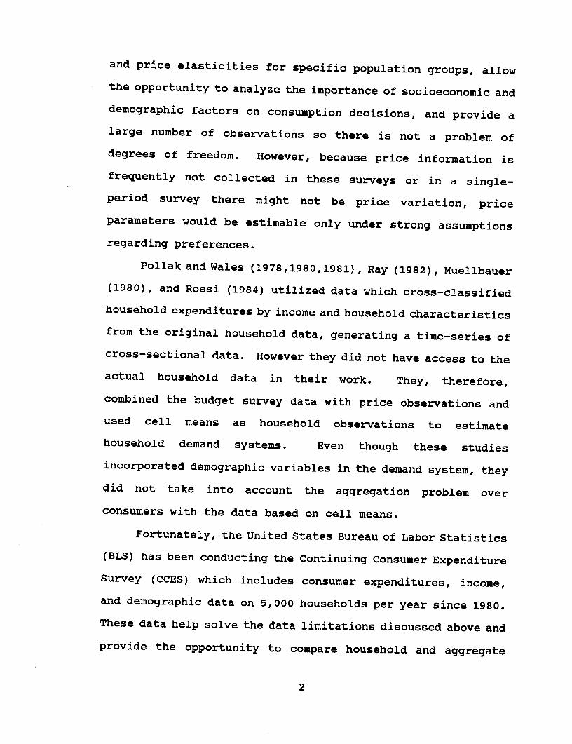
and price elasticities for specific population groups, allow

the opportunity to analyze the importance of socioeconomic and

demographic factors on consumption decisions, and provide a

large number of observations so there is not a problem of

degrees of freedom. However, because price information is

frequently not collected in these surveys or in a single-

period survey there might not be price variation, price

parameters would be estimable only under strong assumptions

regarding preferences.

Pollak and Wales (1978,1980,1981), Ray (1982), Muellbauer

(1980), and Rossi (1984) utilized data which cross-classified

household expenditures by income and household characteristics

from the original household data, generating a time-series of

cross-sectional data. However they did not have access to the

actual household data in their work. They, therefore,

combined the budget survey data with price observations and

used cell means as household observations to estimate

household demand systems. Even though these studies

incorporated demographic variables in the demand system, they

did not take into account the aggregation problem over

consumers with the data based on cell means.

Fortunately, the United States Bureau of Labor Statistics

(BLS) has been conducting the Continuing Consumer Expenditure

Survey (CCES) which includes consumer expenditures, income,

and demographic data on 5,000 households per year since 1980.

These data help solve the data limitations discussed above and

provide the opportunity to compare household and aggregate

2

models. The estimation of demand systems with data both at

the household level and aggregate level will permit us to

compare the estimated demand parameters and study the

empirical implications of aggregation over consumers.

This analysis uses data from eight years of the Diary

portion of the BLS CCES (1980-1987) to estimate a demand

system for six food commodities: cereal and bakery goods,

meats including poultry and fish, dairy products, fruits and

vegetables, other at-home foods, and food away from home.

Price data are not collected in the CCES, nor are quantities

provided. To introduce prices, the Consumer Price Index (CPI)

for each of the above categories was matched with the

household observations by month and region (Northeast, North-

central, South and West). In addition to the household data,

the observations were aggregated by month and region and the

resulting 384 cell means were analyzed for comparison.

After studying various demand models, the Almost Ideal

Demand System (AIDS) was considered the most suitable one for

this study. The iterative Zellner's seemingly unrelated

regression technique was applied to estimate the parameters of

the demand system. In addition, translating procedures were

used to incorporate demographic variables into the complete

demand system.

The plan of this paper is as follows. Section 2 presents

a review of the theory of aggregation. Section 3 introduces

an application of this theory to the Almost Ideal Demand

System and the incorporation of demographic variables. A

3

brief description of the data and estimation procedure is

presented in section 4. Empirical results are presented and

evaluated in section 5. We end with some conclusions in

section 6.

II. AGGREGATION OVER CONSUMERS

"The role of aggregation theory is to provide the

necessary conditions under which it is possible to treat

aggregate consumer behavior as if it were the outcome of the

decisions of a single maximizing consumer"; this is called

"exact aggregation" (Deaton and Muellbauer, 1980b, p. 148).

In the present section different approaches to aggregation

over consumers will be discussed.

Denote qi the demand for good i of household h as

ih fih(XhP) (1)

where xh is the total expenditure of the household, and p is

a price vector. If there are H households, the average demand

q will be

qi = (x x.... xp) = h fih(XhP) (2)

Exact aggregation is possible if we can write (2) as

i = fi(p) (3)

where x is the average total expenditure (Deaton and

Muellbauer, 1990b, p. 150).

Gorman: Parallel Linear Engel Curves

For (3) to hold, Gorman (1961) showed that the individual

cost (expenditure) function must have the form:

4

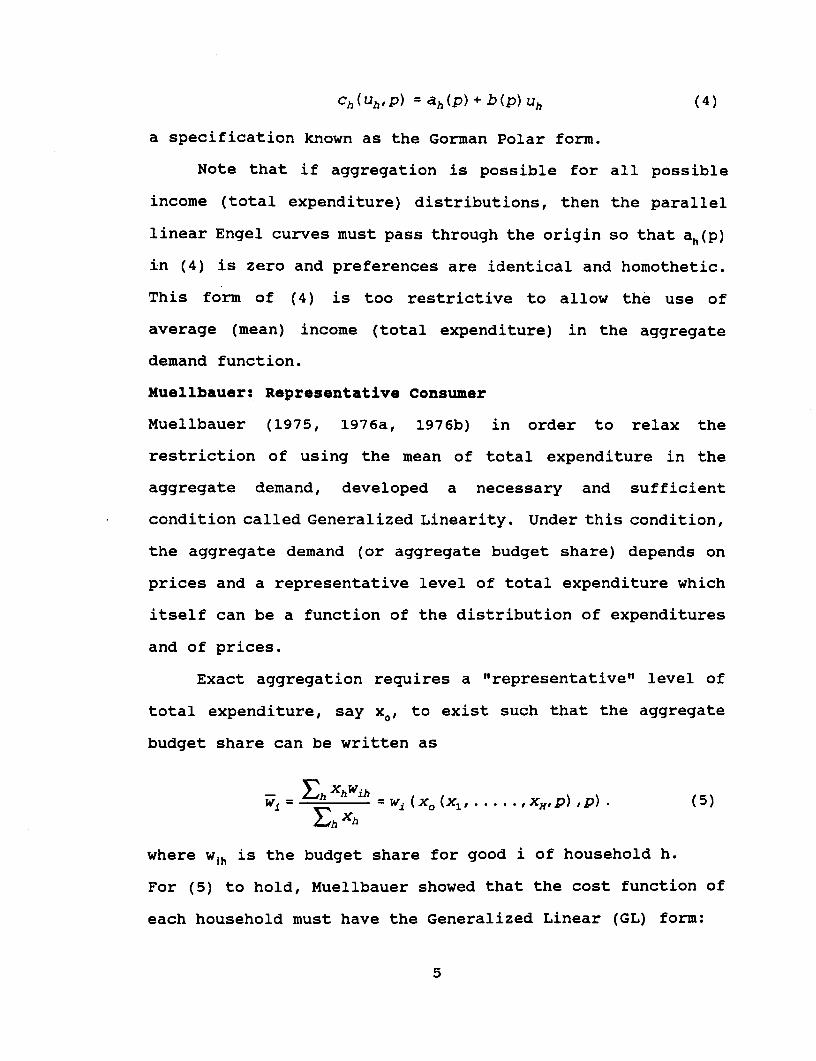
Ch(uh,P) = ah(p)+ b(p) uh (4)

a specification known as the Gorman Polar form.

Note that if aggregation is possible for all possible

income (total expenditure) distributions, then the parallel

linear Engel curves must pass through the origin so that ah(p)

in (4) is zero and preferences are identical and homothetic.

This form of (4) is too restrictive to allow the use of

average (mean) income (total expenditure) in the aggregate

demand function.

Muellbauer: Representative Consumer

Muellbauer (1975, 1976a, 1976b) in order to relax the

restriction of using the mean of total expenditure in the

aggregate demand, developed a necessary and sufficient

condition called Generalized Linearity. Under this condition,

the aggregate demand (or aggregate budget share) depends on

prices and a representative level of total expenditure which

itself can be a function of the distribution of expenditures

and of prices.

Exact aggregation requires a "representative" level of

total expenditure, say xO, to exist such that the aggregate

budget share can be written as

Eh XhWihw, = - = w, (x, (x, ...... ,x,,p) ,p) . (5)

where wih is the budget share for good i of household h.

For (5) to hold, Muellbauer showed that the cost function of

each household must have the Generalized Linear (GL) form:

5

Ch(Uh,p) =Gh(uh,H(p))B(p) +gh(P) (6)

where Shgh(p)=0, H is homogeneous of degree one, and B

homogeneous of degree zero.

A subset of this class is price independent generalized

linearity (PIGL) when the representative expenditure level is

independent of prices and depends only on the distribution of

expenditures (Deaton and Muellbauer, 1980b, pp 155-56). The

cost function of PIGL is

1-1 ~ (7)

Ch(UhP) = kh a (p) (l-uh) +b(p)'Uh] a

where k, and a are scalars. The parameter a is crucial in

determining the nonlinearity of the Engel curves and hence in

determining the relationship between representative and

average expenditures. In Muellbauer's model of the

representative consumer, individual preferences are identical

but not necessarily homothetic.

Lau: Fundamental Theorem of Exact Aggregation

Lau (1982) considered a more general form of aggregation

than that required by expression (3). He considered

individual demand functions of the form fh(xh,p,ah) for total

expenditure Xh, prices p, and attributes (demographic factors)

ah. Lau developed a theory of exact aggregation that makes it

possible to incorporate differences in individual preferences.

The Fundamental Theorem of Exact Aggregation states that under

the assumptions of zero aggregate demand for zero aggregate

expenditure and non-negative individual demand

functions, an aggregate demand function can be written as:

6

h fh(P,x^, ah) =F(p, g(x 1 , .. .,xH a, . . . a,),.,

gK(x 1 , . .. XH,, a,... ,a H)) (8)

if and only if

1)

F(p,gl(xl, * * .Xal, .,a* , .H) .,g a (x,, . ,xH,aj, . . ,aH) ] =

k hk (P) h k (hah) (9)

and,2)

fh(p,x^,a^) =khk(p) g;(xh,a^) for all h (10)

where the index functions g*(x,,ah)=g(xh,ah) - g(O,ah), g(O,ah)

= 0, and gk(.) and hk(p) are linearly independent functions

(Jorgenson, Lau, and Stoker, 1982).

The Gorman parallel linear Engel curves and the

representative consumer conditions are special cases of the

Fundamental Theorem of Exact Aggregation. The former

condition is possible with only one index function while the

latter with two index functions under the assumption of

identical preferences over consumers. This theorem

encompasses more than two indexes and can be applied to

consumers with different preferences.

In this theory the assumption that the impact of

individual expenditures on aggregate demand can be represented

by a single function of individual expenditures, such as

7

aggregate or per capita expenditure, is replaced by the

assumption that there may be a number of such functions.

These functions may depend not only on individual expenditures

but also on attributes of individuals, such as demographic

characteristics, that give rise to differences in preferences.

Thus, it is possible to overcome the limitations of the model

of a representative consumer (Jorgenson, Lau, and Stoker,

1982).

III. AGGREGATION OVER CONSUMERS AND DEMOGRAPHIC VARIABLES IN

AIDS

For the ith commodity the Almost Ideal Demand System of

Deaton and Muellbauer (1980a) takes the following form:

w= a +Pilog(x) + j Yjlogpj (11)

log p:ao Ek klogl = p + Ylgplgp (12)

where w, = pjqi/X is the budget share of the ith commodity whose

price and quantity demanded are given respectively by pi and

qi, X=Epq, (total consumer expenditure or income), and log P

is a price index.

Adding up, homogeneity, and Slutsky restrictions can be

imposed on the system as follows:

1) Ea, = 1;CEYij = Eip,=0 (13)

2) Ejyi = 0 (14)

3) yij = Yji. (15)

For linearity purposes, Stone's price index is used to

approximate log P by log P* = j 1w i log Pi. In which case,

8

equation (11) is known as the Linear Approximate/Almost Ideal

Demand System (LA/AIDS).

Demographic Scaling and the Representative Consumer

Ray's study (1982) is an application of the

representative consumer theory and, at the same time, is the

first research that introduces demographic variables in AIDS,

using the demographic scaling approach. Ray defines the

scale function as kh=N where N represents the number of

household members and the size effect (0).

The household AIDS is

Wih = ai + ilog ( ) + j yiY logpj + ilogNh (16)

where 6S= 08(jyii-PB) and log P is the original price index.

If wi=Ehehwih/Eheh denotes the budget share of the representative

household, where eh is real total expenditure, then

the aqaregate AIDS is

= 'i + Pilog(e) + ¥yj log pj +8ilog N (17)

where i7=ai+Pilog(H/Z)+6ilog(H/Z'), e=Eheh/H, N=EhNh/H; H is the

number of household members; log Z and log Z' are the measure

of expenditure and demographic distributions of the aggregated

households, respectively.

This approach has some limitations: it restricts the size

effect to be identical across commodities; it ignores other

relevant household characteristics (i.e., household composi-

tion); in the aggregate model the expenditure and demographic

distributions of the aggregated households must be assumed

9

constant over time to justify their absorption within the

intercept (not demographic flexibility); and although Ray

estimated both equations (16) and (17) for the household

model, cell means were utilized as household observations.

Demographic Translation and Lau's Theorem of Aggregation

Rossi (1984,1988) applied Lau's theorem to the AIDS,

incorporating demographic variables through the translation

technique (di.=E,6ina, where an are household characteristics).

The household AIDS is

Wih = i + Pi log ( ) +Ej Yijlogpj+ En 5n ah (18)

The price index log P, is approximated by Stone's price index,

log Ph = iWilog Pi'

Adding up, homogeneity, and Slutsky restrictions are

imposed as follows:

1) lia=1l ;EiYi j=E =E i6in=0 (19)

2) Ejyj=0 (20)

3) Yij=Yj.j (21)

The aggregate budget share is

W. _Eh Xh + 2 E Xh P-iog +E YI jlog p^h 2 2h Xh X

*. a ,, 1- i ln (22)

~.=where Z

log P=E ( Xh ) lgpi= w lo g p.

1010

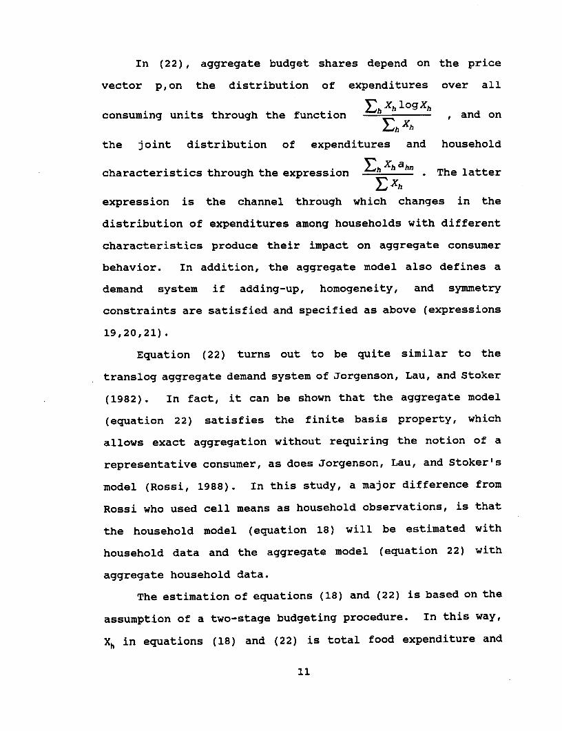
In (22), aggregate budget shares depend on the price

vector p,on the distribution of expenditures over all

C. Xh logXhconsuming units through the function h X, and on

c n Xh

the joint distribution of expenditures and household

Ch Xh acharacteristics through the expression "hX . The latterC Xh

expression is the channel through which changes in the

distribution of expenditures among households with different

characteristics produce their impact on aggregate consumer

behavior. In addition, the aggregate model also defines a

demand system if adding-up, homogeneity, and symmetry

constraints are satisfied and specified as above (expressions

19,20,21).

Equation (22) turns out to be quite similar to the

translog aggregate demand system of Jorgenson, Lau, and Stoker

(1982). In fact, it can be shown that the aggregate model

(equation 22) satisfies the finite basis property, which

allows exact aggregation without requiring the notion of a

representative consumer, as does Jorgenson, Lau, and Stoker's

model (Rossi, 1988). In this study, a major difference from

Rossi who used cell means as household observations, is that

the household model (equation 18) will be estimated with

household data and the aggregate model (equation 22) with

aggregate household data.

The estimation of equations (18) and (22) is based on the

assumption of a two-stage budgeting procedure. In this way,

Xh in equations (18) and (22) is total food expenditure and

11

can be studied separately from the first-stage allocation of

income to food and nonfood expenditure (Phlips, 1974, pp. 66-

74). The Diary CCES does not collect information on total

consumer expenditures. The Interview portion of the CCES

does, but it is a separate survey. Initial work using income

as the independent variable yielded poor results. Income is

notorious for serious measurement error problems.

IV. ESTIMATION PROCEDURE AND DATA

The iterative Zellner's (1962) seemingly unrelated

regression (ITSUR) technique was applied to estimate the

consumption parameters for the household and aggregate models

(equations 18 and 22). The iterative Zellner's estimator is

consistent and asymptotically efficient in the context of a

multivariate normal distribution. In addition, it has the

property that estimates of parameters are invariant to the

choice of equation for deletion (Chalfant 1987). The models

(aggregate and household) will be determined with the adding-

up, homogeneity, and symmetry restrictions imposed.

Because the budget shares sum to one, a demand system

composed of individual expenditure share equations would be

singular. Therefore, one of the equations must be deleted to

estimate the equations as a system. The miscellaneous (other)

food category was chosen for deletion in this study. However,

the parameters for the omitted share equation can be

calculated by using the adding-up restriction from (19).

The aggregation over households creates a problem of

heteroscedasticity. The number of households combined by

12

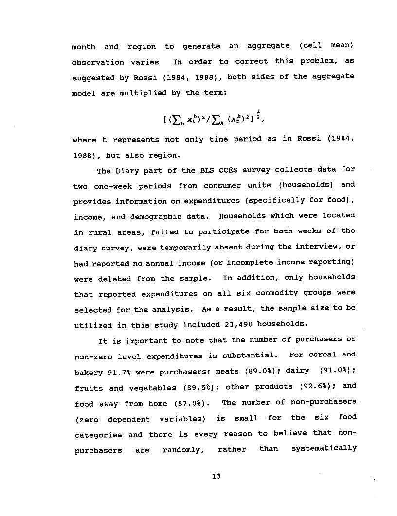
month and region to generate an aggregate (cell mean)

observation varies In order to correct this problem, as

suggested by Rossi (1984, 1988), both sides of the aggregate

model are multiplied by the term:

[(h t ) 2/Eh (Xe)2] 2,

where t represents not only time period as in Rossi (1984,

1988), but also region.

The Diary part of the BLS CCES survey collects data for

two one-week periods from consumer units (households) and

provides information on expenditures (specifically for food),

income, and demographic data. Households which were located

in rural areas, failed to participate for both weeks of the

diary survey, were temporarily absent during the interview, or

had reported no annual income (or incomplete income reporting)

were deleted from the sample. In addition, only households

that reported expenditures on all six commodity groups were

selected for the analysis. As a result, the sample size to be

utilized in this study included 23,490 households.

It is important to note that the number of purchasers or

non-zero level expenditures is substantial. For cereal and

bakery 91.7% were purchasers; meats (89.0%); dairy (91.0%);

fruits and vegetables (89.5%); other products (92.6%); and

food away from home (87.0%). The number of non-purchasers

(zero dependent variables) is small for the six food

categories and there is every reason to believe that non-

purchasers are randomly, rather than systematically

13

determined. Therefore, no bias is introduced by ignoring the

limited dependent variable issue.

The demographic variable included is an adult equivalent

scale for each consumer unit, which is a continuous variable

and combines age, sex, and household size. The adult

equivalent scales were extracted from Tedford, Capps, and

Havlicek (1986).

The prices employed in this study are regional, monthly,

seasonally unadjusted series of the CPI-U for all urban

consumers. Household observations could be matched with the

appropriate CPI data by month and region. The regional CPI

are all set equal to 100 in the base period, and hence do not

reflect price level differences across regions. In order to

capture not only the effect of price level variation across

regions but also geographic effects, regional dummy variables

are introduced in the model.

V. EMPIRICAL RESULTS

Household System

Table 1 presents the parameter estimates of the

restricted household model calculated with 23,490

observations. In general, 52 out of the 72 parameters (74%)

are statistically significant at the 5% level. The system

weighted R2 is .15, which is respectable for household data.

The parameter a is the intercept, the y's are price

coefficients (own and cross), Pi is the coefficient for total

food expenditure, 6,i is the coefficient for adult equivalent

household size, and 6i2 through 6i4 are the regional dummy

14

variable effects for the Northeast, Northcentral, and South

respectively, with the West omitted.

Table 2 provides the uncompensated price, food expen-

diture, and adult equivalent elasticities for the restricted

demand system. The elasticities are evaluated at the means of

the budget share and adult equivalent variable. Most of the

uncompensated own-price elasticities show the anticipated

negative sign. Only the meats category has a positive sign,

but a low price responsiveness. One possible explanation

could be that the price of meats has one of the lowest

variations during the sample period.

The estimated food expenditure elasticities indicate that

five out of six categories are relative necessities1 . The

only category which has a food expenditure elasticity greater

than one is food away from home, as was expected. The meats

category is more expenditure elastic than cereal and bakery

and dairy products. Meats include seafood. This outcome is

in line with expectations.

The adult equivalent elasticities indicate a positive

effect on household consumption of necessities and a negative

influence on luxuries. Food away from home is the only

category with a negative elasticity for adult equivalents.

This result indicates that the larger the household size in

1 The terms "relative" necessity and "relative" luxury will be usedin this study to indicate that some food categories have food expenditureelasticities less than unity or greater than one, respectively. However,we understand that necessity and luxury classifications typically refer toincome or total expenditure elasticities.

15

adult equivalents, the more likely the household would consume

food at home.

Table 3 shows the tests of the restrictions. In all

three tests, the exact F-test and the asymptotic tests: Wald

and Likelihood Ratio (LR), both homogeneity and symmetry are

rejected which is not an unusual result in empirical demand

studies2. Phlips (1974) says there is no reason to be

surprised when empirical demand results do not comply with the

general restrictions. He argues that regardless of such test

results the general restrictions should be imposed since they

"result from the fact that a demand system is obtained by

utility maximization" (Phlips, 1974, pp. 32, 53, and 55).

Aggregate Model by Regions and Time

The aggregate model was estimated using cell means cross-

classified by the four regions and by the month of

observation. The 1980-1987 surveys covered 96 months, so

there are 384 observations (4 regions times 96). The estimated

parameters of the aggregate model, in Table 4, reveal that 74%

of the coefficients are statistically significant. The

restrictions were again imposed. The system weighted R2 is

.98. A high R2 is to be expected with aggregate data.

If the coefficients of the household model in table 1 are

treated as the true parameters (as constants), an F-test can

be used to test the overall equality of the household and

2 Many previous studies that used AIDS reported rejection of theconstraints: Deaton and Muellbauer (1980), Ray (1982), Blanciforti andGreen (1983), Swamy and Binswagner (1983), Rossi (1984), and Eales andUnnevehr (1988).

16

aggregate demand equations in tables 1 and 4. The F-statistic

of 1.20 is below the critical value of 1.40 at the 5 percent

level of significance. Therefore, the hypothesis of equality

can not be rejected3 .

Table 5 presents the uncompensated price, expenditure,

and adult equivalent elasticities for the aggregate

restricted demand system. When compared to the results in

table 2, five of the own-price elasticities are extremely

close and are exactly the same to the nearest hundredth in two

cases. The largest difference exists for meats (.13 vs .29),

and even those estimates are not very far apart. The

expenditure elasticities are all very close; the greatest

dissimilarity is again for meats (.96 vs 1.11), which is

certainly not large. Most of the cross-price elasticities

also compare very favorably as do the adult equivalent

elasticities where the largest difference is for fruits and

vegetables (.001 vs .12).

The own-price and food expenditure elasticities in tables

2 and 5, with the exception of the price elasticity for meats,

are within the general range of the values estimated in

previous U.S. food demand studies (Blanciforti and Green,

1983; Huang, 1985; Huang and Raunikar, 1987; Kokoski, 1986;

Lee, 1990; and Young, 1987).

3 A test which accounts for the variance of the household model as well asthe covariance between the household and aggregate models might be possible basedon a bootstrap or jackknife procedure. However, it imposes a very largecomputational burden (Efron and Gong, 1983 and Efron, 1988).

17

Further Empirical Results

For reasons of length, only a brief discussion of other

relevant empirical findings is presented in this subsection4.

The household and aggregate models were also estimated without

imposing homogeneity and symmetry constraints. The

elasticities of the unrestricted demand systems were less in

accordance with consumer theory and the empirical results of

previous studies, particularly for the aggregate model. For

example, two own-price elasticities were positive in the

aggregate model.

The household model (equation 18) was also estimated with

the aggregate data (the 384 cell means). This approach

ignores the aggregation issue, which is what most previous

demand studies based on time-series data or aggregate (cell

means) household data have done. The results obtained were

similar to those from the household model (equation 18) with

the household data and the aggregate model (equation 22) with

the aggregate data, as reported in tables 1,2,4, and 5.

An F-test was used to test the overall equality of the

household model demand equations estimated with the household

and aggregate data. With an F-statistic of .31 and a critical

value of 1.40 at the 5 percent significance level, the

hypothesis of equality can not be rejected. The estimated

elasticities were also very similar to those shown in table 2.

Although the own-price elasticity of dairy products was

4 These results will be provided by the authors when requested.

18

positive, its magnitude only went from -.07 to +.04, in both

cases very close to zero.

These results support Pollak and Wales' (1980 and 1981)

argument that aggregate data (cell means) can be treated "as

if they were consumption patterns of households" and that

ignoring the aggregation issue is "relatively harmless" (1981,

p. 1541), at least when the demand system is linear in

expenditure. The Linear Approximate AIDS fulfills this

criteria. The aggregation issue might not be so harmlessly

ignored if the demand system is not linear in expenditure

(Pollak and Wales, 1980, p. 600).

An aggregate model with the data classified only by time

period (month), which had 96 cell means as observations, was

also estimated. The national monthly CPI price series were

used in this case. In this case, the test of overall equality

with the household results (table 1) was rejected based on an

F-statistic of 1.72 and a critical value of 1.51 for a 5%

level of significance. The results with this model were very

poor, particularly in terms of price elasticities. Four of

the uncompensated own-price elasticities were positive. The

primary reason is undoubtedly the loss in price variability

without the regional variation in prices. If aggregation

eliminates too much of the variation in the variables, an

aggregate model can not be expected to yield results similar

to the household model, or in line with expectations based on

the theory and previous results.

19

VI. CONCLUSIONS

This study has focused on comparing the performance of

aggregate and household demand models and data, in order to

learn if aggregate consumer behavior is similar to household

consumer behavior and to answer empirically whether the

regression results and demand elasticities with aggregate data

are equivalent to those with household data. To this end a

household demand system based on an extension of the AIDS

model and an aggregate demand system that is not only

theoretically plausible, but also allows distribution of

expenditures among households with different characteristics

and preferences, were presented and estimated. The models

were estimated for six food commodities pooling eight years of

BLS Continuing Consumer Expenditure Survey data and matching

the observations with the CPI price series by month and

region.

The aggregate model yields results equivalent to the

household model based on an F-test of the regression results

and a comparison of the demand elasticities. On the same

basis, the estimates generated by the aggregate data with the

household model also appear equivalent. Two additional

insights were gained from further empirical analysis. The

imposition of the theoretical restrictions (homogeneity and

symmetry) seem to be particularly important for the

performance of the aggregate model. Moreover, a model

estimated with the data aggregated into just 96 monthly

observations performs very poorly. If much of the variability

20

of certain variables is eliminated by aggregation, aggregate

models should not be expected to perform well.

Given the enormous number of demand studies that have

been conducted with aggregate time-series data, the results of

this study are, generally, quite reassuring. Aggregate demand

data may yield empirical results equivalent to those obtained

with disaggregated (household) data. This can hold true not

only for the estimates generated by a theoretically consistent

aggregate demand model, but also for those from a basic

household model estimated with aggregate data. At least for

demand systems that are linear in expenditure, ignoring the

aggregation issue may have minimal consequences and,

therefore, be acceptable.

21

TABLE 1. DEMAND SYSTEM: HOUSEHOLD MODEL

Parameter Estimates (10-2)

Goods 1 2 3 4 5 6

ai 14.84 17.5 16.81 17.81 22.24 10.79

(71.7) (38.1) (78.5) (66.2) (14.0)

Yi.1 6.65

(2.35)

Yiz 0.79 22.0

(0.74) (12.3)

Yi3 -4.94 1.03 8.26

(-3.56) (0.96) (5.5)

Yi4 -1.08 -0.15 1.98 7.80

(-1.14) (-0.15) (2.41) (6.35)

Yi 5 3.04 -0.62 -5.99 -3.08 2.82

(1.32) (-0.35) (-2.9) (-2.27)

Yi6 -4.47 -23.1 -0.35 -5.47 3.83 29.54

(-2.02) (-11.4) (-0.22) (-3.22) (7.18)

Pi -2.41 -0.88 -2.87 -1.77 -1.79 9.73

(-38.1) (-6.25) (-43.8) (-21.5) (41.2)

ail 1.08 1.66 1.16 0.00 0.89 -4.79

(33.6) (23.3) (34.9) (0.08) (-40.1)

bi2 0.85 2.94 0.16 -0.18 -1.70 -2.07

(8.25) (13.5) (1.56) (-1.4) (-5.7)

22

TABLE 1 Continued

Goods 1 2 3 4 5 6

6i3 0.23 1.18 -0.51 -1.15 0.33 -0.09

(2.52) (5.7) (-5.3) (-9.5) (-0.26)

4 ' -0.14 2.55 -1.08 -0.82 -0.46 -0.05

(-1.47) (12.3) (-10.9) (-6.72) (-0.15)

DW 1.97 1.94 1.98 1.97 1.92

Ratio of parameter estimates to standard errors in parentheses. DW:Durbin Watson test. i-i: Cereal & Bakery; i-2: Meats; i-3: Dairy; i-4:Fruits & Vegetables; i-5: Others; i-6: FAFH. System Weighted R2 - 0.15.

23

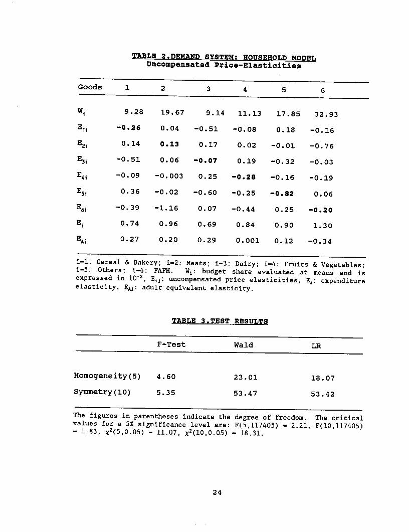
TABLE 2.DEMAND SYSTEM: HOUSEHOLD MODELUncompensated Price-Elasticities

Goods 1 2 3 4 5 6

W i 9.28 19.67 9.14 11.13 17.85 32.93

Eli -0.26 0.04 -0.51 -0.08 0.18 -0.16

E2 i 0.14 0.13 0.17 0.02 -0.01 -0.76

E3, -0.51 0.06 -0.07 0.19 -0.32 -0.03

E4i -0.09 -0.003 0.25 -0.28 -0.16 -0.19

E5 i 0.36 -0.02 -0.60 -0.25 -0.82 0.06

E6J -0.39 -1.16 0.07 -0.44 0.25 -0.20

Ei 0.74 0.96 0.69 0.84 0.90 1.30

EAi 0.27 0.20 0.29 0.001 0.12 -0.34

i-l: Cereal & Bakery; i-2: Meats; i-3: Dairy; i-4: Fruits & Vegetables;i-5: Others; i-6: FAFH. Wi: budget share evaluated at means and isexpressed in 10-2, Ej: uncompensated price elasticities, Ei: expenditureelasticity, EAi: adult equivalent elasticity.

TABLE 3.TEST RESULTS

F-Test Wald LR

Homogeneity(5) 4.60 23.01 18.07

Symmetry(10) 5.35 53.47 53.42

The figures in parentheses indicate the degree of freedom. The criticalvalues for a 5% significance level are: F(5,117405) - 2.21, F(10,117405)- 1.83, X2(5,0.05) - 11.07, X2(10,0.05) - 18.31.

24

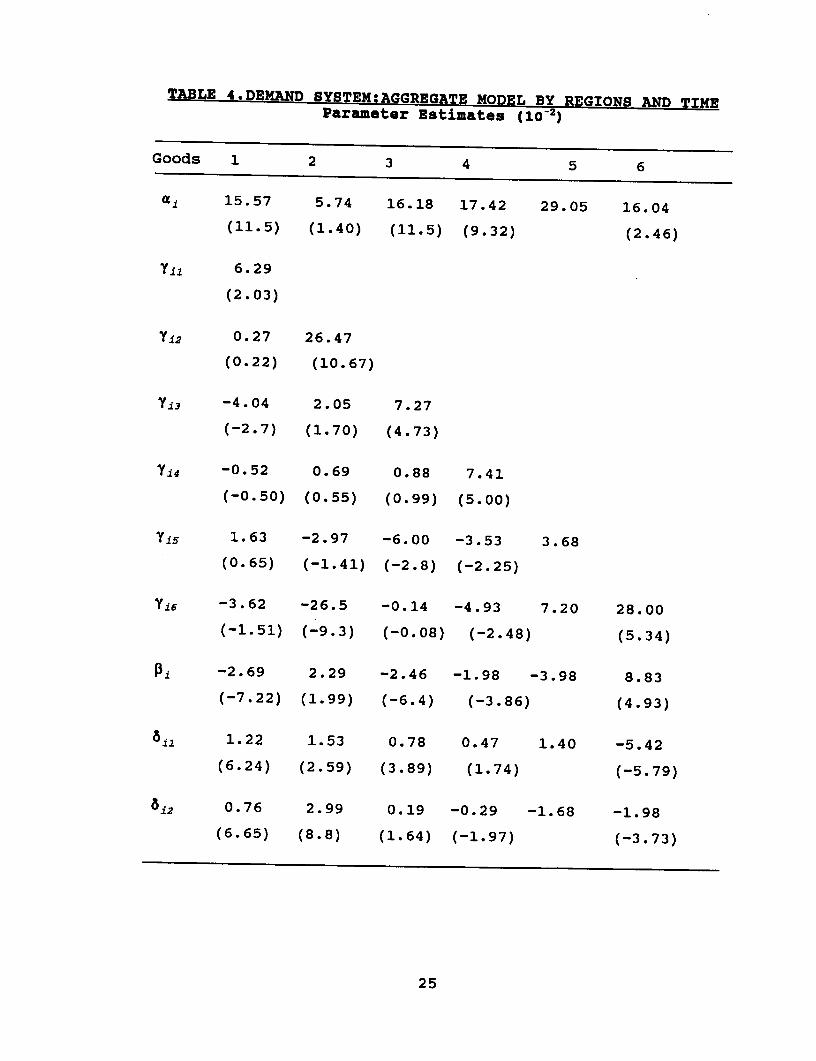
TABLE 4.DEMAND SYSTEM:AGGREGATE MODEL BY REGIONS AND TIMEParameter Estimates (10 -2)

Goods 1 2 3 4 5 6

a i 15.57 5.74 16.18 17.42 29.05 16.04

(11.5) (1.40) (11.5) (9.32) (2.46)

Yii 6.29

(2.03)

Yi2 0.27 26.47

(0.22) (10.67)

Yi3 -4.04 2.05 7.27

(-2.7) (1.70) (4.73)

Yi4 -0.52 0.69 0.88 7.41

(-0.50) (0.55) (0.99) (5.00)

Yis 1.63 -2.97 -6.00 -3.53 3.68

(0.65) (-1.41) (-2.8) (-2.25)

Yi6 -3.62 -26.5 -0.14 -4.93 7.20 28.00

(-1.51) (-9.3) (-0.08) (-2.48) (5.34)

Pi -2.69 2.29 -2.46 -1.98 -3.98 8.83

(-7.22) (1.99) (-6.4) (-3.86) (4.93)

ail 1.22 1.53 0.78 0.47 1.40 -5.42

(6.24) (2.59) (3.89) (1.74) (-5.79)

iz2 0.76 2.99 0.19 -0.29 -1.68 -1.98

(6.65) (8.8) (1.64) (-1.97) (-3.73)

25

TABLE 4 Continued

Goods 1 2 3 4 5 6

8i3 0.15 1.69 -0.43 -1.21 0.22 -0.41

(1.30) (4.78) (-3.7) (-7.7) (-0.74)

6i4 -0.27 2.66 -0.94 -0.91 -0.62 0.08

(-2.3) (7.80) (-8.08) (-5.92) (0.15)

DW 1.72 1.76 1.90 1.76 1.71

Ratio of parameter estimates to standard errors in parentheses. DW:Durbin Watson test. i-i: Cereal & Bakery; i-2: Meats; i-3: Dairy; i-4:Fruits & Vegetables; i-5: Others; i-6: FAFH. System Weighted R2 - 0.98.

26

TABLE 5.DEMAND SYSTEM:AGGREGATE MODEL BY REGIONS AND TIMEUncompensated Price-Elasticities

Goods 1 2 3 4 5 6

W i 8.83 20.08 8.59 10.59 17.23 34.68

Eli -0.26 0.003 -0.45 -0.03 0.11 -0.13

E2i 0.09 0.29 0.30 0.10 -0.13 -0.82

Ei -0.43 0.09 -0.13 0.10 -0.33 -0.03

E4, -0.03 0.02 0.13 -0.28 -0.18 -0.17

E5 i 0.24 -0.17 -0.65 -0.30 -0.75 0.16

E6 i -0.30 -1.36 0.08 -0.40 0.49 -0.28

E i 0.70 1.11 0.71 0.81 0.77 1.25

E^i 0.37 0.21 0.24 0.12 0.22 -0.41

i-i: Cereal & Bakery; i-2: Meats; i-3: Dairy; i-4: Fruits & Vegetables;i-5: Others; i-6: FAFH. Wi: budget share evaluated at means and isexpressed in 10-2, Eij: uncompensated price elasticities, Ei: expenditure

elasticity, EAi: adult equivalent elasticity.

27

REFERENCES

Blanciforti, L. and R. Green. "The Almost Ideal Demand System:Comparison and Applications to Food Groups." AgriculturalEconomics Research 35(1983): 1-10.

Chalfant, J.A. "A Globally Flexible Almost Ideal DemandSystem." Journal of Business and Economic Statistics 5(1987):233-42.

Deaton, A. and J. Muellbauer. "Almost Ideal Demand System,"American Economic Review 70(1980a): 312-26.

Deaton, A. and J. Muellbauer. Economics and Consumer Behavior.Cambridge: 1980b.

Eales, J. and L.J. Unnevehr. "Demand for Beef and ChickenProducts: Separability and Structure Change." AmericanJournal of Agricultural Economics 70(1988): 521-32.

Efron, B. "Better Bootstrap Confidence Intervals." Journalof the American Statistician Association 82(1988): 171-200.

Efron, B. and G. Gong. "A Leisurely Look at the Bootstrap,the Jackknife, and Cross-Validation," The AmericanStatistician 37(1983): 36-48.

Gorman, W.M. "On a Class of Preference Fields."Metroeconomica 13(1961): 53-56.

Hammond, J. and R. Todd. "Accounting for Cross Demand Effectsin Dairy Product Consumption Forecasts." USDA, ERS, CEDworking paper, Washington D.C., 1974.

Huang, C. and R. Raunikar. "Food Expenditure PatternsEvidence from U.S. Household Data," in 0. Capps and B. Senauer(eds.), Food Demand Analysis. Department of AgriculturalEconomics, Virginia Polytechnic Institute and StateUniversity, 1987.

Huang, K. "U.S. Demand for Food: A Complete System of Priceand Income Effects." USDA,ERS, Technical Bulletin No 1714,Washington D.C., 1985.

Jorgenson, D., L. Lau, and T. Stoker. "The TranscendentalLogarithmic Model of Aggregate Consumer Behavior," in R.Basmann and G. Rhodes (eds.), Advances in Econometrics, Vol 1.London: Aijai Press Inc., 1982.

28

Kokoski, M.F. "An Empirical Analysis of Intertemporal andDemographic Variations in Consumer Preferences." AmericanJournal of Agricultural Economics 68(1986): 894-907.

Lau, L. "A Note on the Fundamental Theorem of ExactAggregation." Economics Letters 9(1982): 119-126.

Lee, H. J. "Nonparametric and Parametric Analyses for FoodDemand in the United States." Ph.D. Dissertation, The OhioState University, 1990.

Muellbauer, J. "Aggregation, Income Distribution, andConsumer Demand." Review of Economics Studies 42(1975): 525-43.

Muellbauer, J. "Community Preferences and the RepresentativeConsumer." Econometrica 44(1976a): 979-99.

Muellbauer, J. "Economics and the Representative Consumer,"in L. Solari and J.N. Du Pasquier (eds.), Private and EnlargedConsumption. Amsterdam: North Holland, 1976b.

Muellbauer, J. "The Estimation of the Prais-Houthakker Modelof Equivalence Scales." Econometrica 48(1980): 153-76.

Phlips, L. Applied Consumption Analysis. NorthHolland/American Elsevier: 1974.

Pollak, R.A. and T.J. Wales. "Estimation of Complete DemandSystems from Household Budget Data: The Linear and QuadraticExpenditure Systems." American Economic Review 68(1978): 348-54.

Pollak, R.A. and T.J. Wales. "Comparison of the QuadraticExpenditure System and Translog Demand System with AlternativeSpecifications of Demographic Effects." Econometrica48(1980): 592-612.

Pollak, R.A. and T.J. Wales. "Demographic Variables in DemandAnalysis." Econometrica 49(1981): 1533-44.

Ray, R. "The Testing and Estimation of Complete DemandSystems on Household Budget Surveys." European EconomicReview 17(1982): 349-69.

Rossi, N. "Consumers' Demand in Italy 1970-1980." Ph.D.Dissertation, London School of Economics, 1984.

Rossi, N. "Budget Share Demographic Translation and theAggregate Almost Ideal Demand System." European EconomicReview 32(1988): 1301-18.

29

Swamy, G. and H.P. Binswanger. "Flexible Consumer Demand

Systems and Linear Estimation: Food in India." American

Journal of Agricultural Economics 65(1983): 675-84.

Tedford, J.R., O. Capps Jr., and J. Havlicek Jr. "Adult

Equivalent Scales Once More-A Development Approach." American

Journal of Agricultural Economics 68(1986): 322-33.

Young, N.C. "Prior Information in Demand System Estimation."

Ph.D. Dissertation, University of Minnesota, 1987.

Zellner, A. "Efficient Method of Estimating Seemingly

Unrelated Regressions and Tests for Aggregation Bias."

Journal of the American Statistical Association 57(1962): 348-

68.

30