CEP Discussion Paper No 786

April 2007

Seigniorage

Willem Buiter

Abstract Governments through the ages have appropriated real resources through the monopoly of the ‘coinage’. In modern fiat money economies, the monopoly of the issue of legal tender is generally assigned to an agency of the state, the Central Bank, which may have varying degrees of operational and target independence from the government of the day.

In this paper I analyse four different but related concepts, each of which highlights some aspect of the way in which the state acquires command over real resources through its ability to issue fiat money. They are (1) seigniorage (the change in the monetary base), (2) Central Bank revenue (the interest bill saved by the authorities on the outstanding stock of base money liabilities), (3) the inflation tax (the reduction in the real value of the stock of base money due to inflation and (4) the operating profits of the central bank, or the taxes paid by the Central Bank to the Treasury.

To understand the relationship between these four concepts, an explicitly intertemporal approach is required, which focuses on the present discounted value of the current and future resource transfers between the private sector and the state. Furthermore, when the Central Bank is operationally independent, it is essential to decompose the familiar consolidated ‘government budget constraint’ and consolidated ‘government intertemporal budget constraint’ into the separate accounts and budget constraints of the Central Bank and the Treasury. Only by doing this can we appreciate the financial constraints on the Central Bank’s ability to pursue and achieve an inflation target, and the importance of cooperation and coordination between the Treasury and the Central Bank when faced with financial sector crises involving the need for long-term recapitalisation or when confronted with the need to mimic Milton Friedman’s helicopter drop of money in an economy faced with a liquidity trap. Key Words: inflation tax; central bank budget constraint; coordination of monetary and fiscal policy JEL Classifications: E4, E5, E6, H6 This paper was produced as part of the Centre’s Macro Programme. The Centre for Economic Performance is financed by the Economic and Social Research Council. Acknowledgements I would like to thank Charles Goodhart, Michael Bordo, Marc Flandreau and Anne Sibert for helpful comments. Willem Buiter is a Research Associate with the Macro Programme, Centre for Economic Performance, London School of Economics. He is also Chair of European Political Economy, European Institute, LSE. Published by Centre for Economic Performance London School of Economics and Political Science Houghton Street London WC2A 2AE All rights reserved. No part of this publication may be reproduced, stored in a retrieval system or transmitted in any form or by any means without the prior permission in writing of the publisher nor be issued to the public or circulated in any form other than that in which it is published. Requests for permission to reproduce any article or part of the Working Paper should be sent to the editor at the above address. © W. Buiter, submitted 2007 ISBN 978 0 85328 161 0

1

I. Introduction

Seigniorage refers historically, in a world with commodity money, to the difference

between the face value of a coin and its costs of production and mintage. In fiat money

economies, the difference between the face value of a currency note and its marginal printing cost

are almost equal to the face value of the note – marginal printing costs are effectively zero.

Printing fiat money is therefore a highly profitable activity – one that has been jealously regulated

and often monopolized by the state.

Although the profitability of printing money is widely recognized, the literature on the

subject contains a number of different measures of the revenue appropriated by the state through

the use of the printing presses. In this paper, I discuss four of them and consider the relationship

between them in an intertemporal setting. There also is the empirical institutional regularity, that

the state tends to assign the issuance of fiat money to a specialized agency, the Central Bank,

which has some degree of independence from the other organs of the state and from the

government administration of the day. This institutional arrangement has implications for the

conduct of monetary policy that cannot be analysed in the textbook macroeconomic models,

which consolidate the Central Bank with the rest of the government.

In the next four Sections, the paper addresses the following four questions. (1) What

resources does the state appropriate through the issuance of base money (currency and

commercial bank balances with the Central Bank)? (2) What inflation rate would result if the

monetary authority were to try to maximise these resources? (3) Who ultimate appropriates and

benefits from these resources, the Central Bank or the Treasury/Ministry of Finance? (4) Does the

Central Bank have adequate financial resources to pursue its monetary policy mandate (taken to

be price stability) and its financial stability mandate. Specifically, for inflation-targeting Central

2

Banks, is the inflation target financeable? The first two questions receive preliminary answers in

Section II of the paper, confirming results that can be found e.g. in Walsh (2003) and Romer

(2006). The second half of Section II contains an analysis of the relationship between three of

base money issuance revenue measures (seigniorage, central bank revenue and the inflation tax)

in real time, that is, outside the steady state and without the assumptions that the Fisher

hypothesis holds and that the velocity of circulation of base money is constant over time. It

derives the ‘intertemporal seigniorage identity’ relating the present discounted value of

seigniorage and the present discounted value of Central Bank revenue.

The government’s period budget constraint and its intertemporal budget constraint have

been familiar components of dynamic macroeconomic models at least since the late 1960s (see

e.g. Christ (1968), Blinder and Solow (1973) and Tobin and Buiter (1976)). The ‘government’ in

question is invariably the consolidated general government (central, state and local, henceforth

the ‘Treasury’) and Central Bank. When the Central Bank has operational independence, it is

useful, and at times even essential, to disaggregate the general government accounts into separate

Treasury and Central Bank accounts. Section III of the paper presents an example of such a

decomposition, extending the analysis of Walsh (2003). In Section IV, a simple dynamic general

equilibrium model with money is presented, which incorporates the Treasury and Central Bank

whose accounts were constructed in Section III. It permits all four questions to be addressed.

Section V raises two further issues prompted by the decomposition of the government’s accounts

into separate Central Bank and Treasury accounts: the need for fiscal resources to recapitalise an

financially stretched or even insolvent Central Bank and the institutional modalities of ‘helicopter

drops of money’.

3

The analysis of the sources of Central Bank revenue or seigniorage is part of a tradition

that is both venerable and incomplete. It starts (at least) with Thornton (1802) and includes such

classics as Bresciani-Turroni (1937) and Cagan (1956). Milton Friedman (1971), Phelps (1973),

Sargent (1982, 1987) and Sargent and Wallace (1981) have made important contributions.

Empirical investigations include King and Plosser (1985), Dornbusch and Fischer (1986), Anand

and van Wijnbergen (1989), Buiter (1990), Kiguel and Neumeyer (1995) and Easterly, Mauro

and Schmidt-Hebbel (1995). Recent theoretical investigations include Sims (2004, 2005) and

Buiter (2004, 2005). Modern advanced textbooks/treatises such as Walsh (2003 and Romer

(2006) devote considerable space to the issue. The explicitly multi-period or intertemporal

dimension linking the various notions of seigniorage has not, however, been brought out and

exploited before.

II. Three faces of seigniorage

There are two common measures of ‘seigniorage’, the resources appropriated by the

monetary authority through its capacity to issue zero interest fiat money. The first, 1S , is the

change in the monetary base, 1, 1t t t tS M M M −= ∆ = − , where tM is the stock of nominal base

money outstanding at the end of period t and the beginning of period 1.t − The term

seigniorage is sometimes reserved for this measure (see e.g. Flandreau (2006), and Bordo (2006))

and I shall follow this convention, although usage is not standardised. The second measure, 2S ,

is the interest earned by investing the resources obtained though the past issuance of base money

in interest-bearing assets: 2, , 1 1t t t tS i M− −= , where , 1t ti − is the risk-free nominal interest rate on

financial instruments other than base money between periods t-1 and t. Flandreau refers to this as

Central Bank revenue and again I shall follow this usage.

4

It is often helpful to measure seigniorage and Central Bank revenue in real terms or as a

share of GDP. Period t seigniorage as a share of GDP, 1,ts , is defined as 1,t

tt t

MsPY∆= and period t

Central Bank revenue as a share of GDP, 2,ts , as 12, , 1

tt t t

t t

Ms iPY

−−= , where tP is the period t price

level and tY period t real output.

A distinct but related concept to seigniorage and Central Bank revenue is the inflation

tax, 3S . The inflation tax is the reduction in the real value of the stock of base money caused by

inflation.1 Let , 11

1tt t

t

PP

π −−

= − be the rate of inflation between periods t-1 and t, then the period t

inflation tax is 3, , 1 1t t t tS Mπ − −= . The inflation tax as a share of GDP will be denoted

13, , 1

tt t t

t t

MsPY

π −−= .

Let , 11

1tt t

t

YY

γ −−

= − be the growth rate of real GDP between periods t-1 and t. The real

interest rate between periods t-1 and t is denoted , 1t tr − where

, 1 , 1 , 1(1 )(1 ) 1t t t t t tr iπ− − −+ + = + (1)

The growth rate of the nominal stock of base money between periods t-1 and t is denoted

, 11

1tt t

t

MM

µ −−

= − . Finally, let the ratio of the beginning-of-period base money stock to nominal

GDP in period t be denoted 1tt

t t

MmPY

−= .

1 This is sometimes called the ‘anticipated inflation tax’, to distinguish it from the ‘unanticipated inflation tax’, the reduction in the real value of outstanding fixed interest rate nominally denominated debt instruments caused by an unexpected increase in the rate of inflation which causes their price and real value to decline.

5

Steady-state seigniorage

Assume that in a deterministic steady state, the ratio of base money to nominal GDP is

constant, that is,

1 (1 )(1 )µ π γ+ = + + (2)

where variables with overbars denote deterministic steady-state values. In steady state,

1

2

3

s ms ims m

µ

π

===

or, using (1) and (2)

( )( )

1

2

3

(1 )(1 ) 1

(1 )(1 ) 1

s m

s r ms m

π γπ

π

= + + −

= + + −=

(3)

Let ( )( )( )πη ππ

′≡ − l

l be the semi-elasticity of long-run money demand with respect to the

inflation rate. In what follows I will only consider steady-state money demand functions

( ), ' 0m π= <l l that have the property that , 1, 2,3is i = is continuously differentiable, increasing

in π when 0rπ γ= = = and has a unique maximum.2 Such unimodal long-run seigniorage

Laffer curves are consistent with the available empirical evidence (see Cagan (1956), Anand and

van Wijnbergen (1989), Easterly, Mauro and Schmidt-Hebbel (1995) and Kiguel and Neumeyer

(1995)).

2 For 1s this means that for 1

ˆπ π< , ( )(1 )(1 ) 1 ( ) 1π γ η π γ+ + − < + and for 1ˆπ π> ,

( )(1 )(1 ) 1 ( ) 1π γ η π γ+ + − > + . For 2s this means that for 2ˆπ π< , ( )(1 )(1 ) 1 ( ) 1r rπ η π+ + − < + and

for 2ˆπ π> , ( )(1 )(1 ) 1 ( ) 1r rπ η π+ + − > + . For 3s this means that for 3

ˆπ π< , ( ) 1πη π < and that for

3ˆπ π> , ( ) 1πη π > , the familiar condition that when price falls total revenue increases (decreases) if and only if

the price elasticity of demand is less than (greater than) one.

6

I will also assume that the long-run money demand function has the property that the

semi-elasticity of long-run money demand with respect to the inflation rate is non-decreasing:

( ) 0η π′ ≥ ; this is, again, a property shared by the empirically successful base money demand

functions. Probably the most familiar example is the semi-logarithmic long-run base money

demand function, made popular by Cagan’s studies (Cagan (1956)) of hyperinflations, with its

constant semi-elasticity of money demand ( ( )η π η= ):

ln

0m α ηπ

η= −

> (4)

Taking steady state output growth as exogenous, the constant inflation rate that

maximises steady-state seigniorage as a share of GDP is given by:

( )11

1ˆ arg max (1 )(1 ) 1 ( ) ˆ 1( )f γπ π γ π

γη π= + + − = −

+ (5)

Taking the steady-state real rate of interest as given, the constant inflation rate that maximises

steady-state Central Bank revenue as a share of GDP is given by:

( )22

1ˆ arg max (1 )(1 ) 1 ( ) ˆ 1( )rr f

rπ π π

η π= + + − = −

+ (6)

The constant inflation rate that maximises steady-state inflation tax revenue as a share of

GDP is given by

33

1ˆ arg max ( ) 1ˆ( )fπ π π

η π= = − (7)

The following proposition follows immediately:

Proposition 1:

Assume that the long-run seigniorage Laffer curve is increasing at 0π = and unimodal and that the semi-elasticity of money demand with respect to the inflation rate is non-decreasing in the inflation rate. The inflation rate that maximises steady-state seigniorage as a share of GDP is lower than the inflation rate that maximises steady-state Central Bank revenue as a share of GDP if and only if the growth rate of

7

real GDP is greater than the real interest rate. The inflation rate that maximises the steady-state inflation tax as a share of GDP is higher than the inflation rate that maximises steady-state seigniorage as a share of GDP (Central Bank revenue as a share of GDP) if and only if the growth rate of real GDP (the real interest rate) is positive.3

Corollary 1:

The ranking of the maximised values of 1s , 2s and 3s is the same as the ranking of

the magnitudes of 1π̂ , 2π̂ and 3π̂ .

Seigniorage in real time

I shall generalise these three measures of Central Bank resource appropriation to allow

for a non-zero risk-free nominal interest rate on base money, , 1Mt ti − for the rate on base money

between periods t-1 and t. This generalised seigniorage measure is defined by

1, , 1 1(1 )Mt t t t tS M i M− −= − + and the generalised measure of Central Bank revenue is defined by

( )2, , 1 , 1 1M

t t t t t tS i i M− − −≡ −

Expressed as shares of GDP, these two seigniorage measures become:

3 It suffices to show that 1π̂ is decreasing in γ . Since ( )

( )

2211

2

1 1

ˆ( )ˆ 11 ˆ ˆ( ) ( )

dd

η ππγ γ η π η π

⎛ ⎞⎛ ⎞ ⎜ ⎟= −⎜ ⎟ ⎜ ⎟+⎝ ⎠ ⎜ ⎟′ +⎝ ⎠

, 0η′ ≥ is

sufficient but not necessary for the result. This result applies to a large number of empirically plausible base money demand functions. For the linear demand function found e.g. in Sargent and Wallace’s Unpleasant Monetarist Arithmetic model (Sargent and Wallace (1981)) (1 ), 0, 0m mα β π β= − + > > , for instance, we have

( )( )11 1ˆ arg max (1 )(1 ) 1 (1 ) 12 1

απ π γ α β πβ γ

⎛ ⎞= + + − − + = + −⎜ ⎟+⎝ ⎠,

( ) ( )21 1ˆ arg max (1 )(1 ) 1 (1 ) 12 1

rr

απ π α β πβ

⎛ ⎞= + + − − + = + −⎜ ⎟+⎝ ⎠ and

( )31ˆ arg max (1 ) 1 12

απ π α β πβ

⎛ ⎞= − + = + −⎜ ⎟⎝ ⎠

. Proposition 1 applies here also, with

( )(1 )βη π

α β π=

− +.(see Buiter (1990)).

8

, 1 11,

(1 )Mt t t t

tt t

M i Ms

PY− −− +

≡

and

12, , 1 , 1( )M t

t t t t tt t

Ms i iPY

−− −≡ −

The following notation will be needed to define the appropriate intertemporal relative

prices or stochastic discount factors: 1 0,t tI is the nominal stochastic discount factor between

periods 1t and 0t , defined by

1

1 0

0

, , 1 1 01

1 0

for

1 for t

t

t t k kk t

I I t t

t

−= +

= >

= =

∏

The interpretation of 1 0,t tI is the price in terms of period 0t money of one unit of money in

period 1 0t t≥ . There will in general be many possible states in period 1t , and period 1t money has

a period 0t (forward) price for each state. Let tE be the mathematical expectation operator

conditional on information available at the beginning of period t . Provided earlier dated

information sets do not contain more information than later dated information sets, these

stochastic discount factors satisfy the recursion property

( )0 1 0 1 2 1 0 2 0, , , 2 1 0for t t t t t t t t tE I E I E I t t t= ≥ ≥

Finally, the risk-free nominal interest rate in period t, 1,t ti + , that is, the money price in

period t of one unit of money in every state of the world in period t+1 is defined by

1,1,

11 t t t

t t

E Ii +

+

=+

(8)

9

For future reference I also define the real stochastic discount factor between periods 0t

and 1t , 1 0,t tR . Let the inflation factor between period 0t and 1t ,

1 0,t tΠ , be defined by

11

1 0

00

, , 1 1 01

1 0

(1 ) for

1 for

tt

t t k kk tt

Pt t

P

t t

π −= +

Π = = + >

= =

∑

The real stochastic discount factor is defined by

1 0 1 0 1 0, , ,t t t t t tR I= Π

It is easily checked that it has the same recursive properties as the nominal discount factor:

1

1 0

0

, , 1 1 01

1 0

for

1 for t

t

t t k kk t

R R t t

t

−= +

= >

= =

∏

( )0 1 0 1 2 1 0 2 0, , , 2 1 0for t t t t t t t t tE R E R E R t t t= ≥ ≥

The risk-free real rate of interest between periods t and t+1 , 1,t tr + , is defined as

1,1,

11 t t t

t t

E Rr +

+

=+

.

Note that the real GDP growth-corrected discount factors satisfy:

( ) ( )0 1 0 1 0 1 2 1 2 1 0 2 0 2 0, , , , , , 2 1 0for t t t t t t t t t t t t t t tE R Y E R Y E R Y t t t⎡ ⎤ = ≥ ≥⎣ ⎦

The Intertemporal Seigniorage Identity

Acting in real time, the monetary authority will be interested in the present discounted

value of current and future seigniorage, rather than in just its current value or its steady-state

value. A focus on the current value alone would be myopic and an exclusive concern with steady

state seigniorage would not be a appropriate if the traverse to the steady state is non-

10

instantaneous and involves transitional seigniorage revenues that are different from their steady

state values. The present discounted value of the nominal value of seigniorage is given by:

( )1 , , 1 1( ) (1 )Mt t j t j j j j

j t

PDV S E I M i M∞

− −=

≡ − +∑ (9)

The present discounted value of nominal Central Bank revenue is given by:

( )

2 , 1, 1,

, 1, 1 1,

( ) ( )

(1 )

Mt t j t j j j j j

j t

Mt j t j t j j j

j t

PDV S E I i i M

E I I i M

∞

+ +=

∞

+ − +=

≡ −

= − +

∑

∑ (10)4

Through the application of brute force (or in continuous time, through the use of the

formula for integration by parts), and using the second equality in (10), it is easily established

that the following relationship holds identically (see Buiter (1990)):

( ) ( ), , 1 1 , 1, 1, , 1 1

,

(1 ) ( ) 1

lim

M M Mt j t j j j j t j t j j j j j t t t

j t j t

t N t NN

E M i M E I i i M i M

E I M

∞ ∞

− − + + − −= =

→∞

Ι − + ≡ − − +

+

∑ ∑ (11)

I will refer to (11) as the ‘intertemporal seigniorage identity’ or ISI.

If we impose the boundary condition that the present value of the terminal base money

stock is zero in the limit as the terminal date goes to infinity, that is,

,lim 0t N t NNE I M

→∞= , (12)

the ISI becomes

4 The equality of the last two expressions in (10) is established as follows. For 1j t≥ + ,

( ) ( )1, , , 1 1 1, , 1 , 1 1(1 ) 1 (1 )M Mt j t j t j j j t j t j j j j jE I I i M E I I i M− − − − − − −− + = − + . Therefore,

( ) ( )1, , 1 , 1 1 1, 1 , 1 , 1 11 (1 ) 1 (1 )M Mt j t j j j j j t j t j j j j j jE I I i M E I E I i M− − − − − − − − −− + = − + . From (8)

( ) ( )11, 1 , 1 , 1 1 1, , 1 , 1 11 (1 ) 1 (1 ) (1 ) .M M

t j t j j j j j j t j t j j j j jE I E I i M E I i i M−− − − − − − − − −− + = − + +

11

( ) ( )

( )

, , 1 1 , 1, 1, , 1 1

1 2 , 1 1

(1 ) ( ) 1

( ) ( ) 1

or

M M Mt j t j j j j t j t j j j j j t t t

j t j t

Mt t t t t

E M i M E I i i M i M

PDV S PDV S i M

∞ ∞

− − + + − −= =

− −

Ι − + = − − +

= − +

∑ ∑ (13)

There are no additional interesting relationships that can be established between the

inflation tax and the other two monetary resource appropriation measures – seigniorage and

Central Bank revenue, beyond the familiar identity that seigniorage revenue as a share of GDP

equals the inflation tax plus the ‘real growth bonus’ (that is, the increase in the demand for real

money balances associated, cet. par. with real GDP growth) plus the change in the ratio of base

money to GDP:

( )1, 1 1, 1, 1 11 (1 )tt t t t t t t t t

t t

M m m mPY

π γ π+ + + + + +∆ = + + + + ∆ (14)5

When the nominal interest rate on base money is zero, (13) becomes:

, , 1, 1

1 2 1( ) ( )

t j t j t j t j j j tj t j t

t t t

E M E I i M M

PDV S PDV S M

∞ ∞

+ −= =

−

Ι ∆ = −

= −

∑ ∑or (15)

5 Consider, for sake of brevity, the continuous time analogue of (14): ( )m m mµ π γ= + + & .

Taking present discounted values on both sides of this relationship yields:

[ ( ) ( )] [ ( ) ( )] [ ( ) ( )]( ) ( ) [ ( ) ( )] ( ) ( )

s s s

t t tr u u du r u u du r u u du

t t t

e s m s ds e s s m s e m s dsγ γ γ

µ π γ∞ ∞ ∞

− − − − − −∫ ∫ ∫= + +∫ ∫ ∫ & . Applying

integration by parts to the second term on the r.h.s. of the last equation yields

[ ( ) ( )] [ ( ) ( )]( ) ( ) [ ( ) ( )] ( ) ( )

s s

t tr u u du r u u du

t t

e s m s ds e s r s m s m tγ γ

µ π∞ ∞

− − − −∫ ∫= + −∫ ∫ . With

( ) ( ) ( )r s s i sπ+ = , this is simply the continuous time version of the ISI.

12

When there is no uncertainty, (15) simplifies to:

, 1 1 111 1, 1 , 1

1 11 1

j j

j j j j tj t j tk t k tk k k k

M i M Mi i

∞ ∞

− − −= = += + = +− −

∆ ≡ −+ +∑ ∑∏ ∏ (16)

When the risk-free nominal interest rate is constant from period t on, this further simplifies to:

1 11

1 11 1

j t j t

j j tj t j t

M i M Mi i

− −∞ ∞

− −= = +

⎛ ⎞ ⎛ ⎞∆ = −⎜ ⎟ ⎜ ⎟+ +⎝ ⎠ ⎝ ⎠∑ ∑

Using real GDP units as the numéraire rather than money, the ISI in equation (13)

becomes

, 1 1, , , , 1, 1, , 1

1, 2, , 1

(1 )( ) (1 )

(1 )

Mj j j j M M

t j t j t t j t j t j j j j j t t tj t j tj j

Mt t t t t

M i ME R E R i i m i m

P Y

i mσ σ

∞ ∞− −

+ + −= =

−

⎛ ⎞− +Γ = Γ − − +⎜ ⎟⎜ ⎟

⎝ ⎠

= − +

∑ ∑or (17)

Where

, 1 11, 1 , ,

2, 2 , , 1, 1,

(1 )( )

( ) ( )

Mj j j j

t t t j t j tj t j j

Mt t t j t j t j j j j j

j t

M i MPDV s E R

P Y

PDV s E R i i m

σ

σ

∞− −

=

∞

+ +=

⎛ ⎞− += = Γ ⎜ ⎟⎜ ⎟

⎝ ⎠

= = Γ −

∑

∑ (18)

With a zero nominal interest rate on base money, (17) becomes (19):

, , 1, 1, 1,j

t j t j t t j t j t j j j tj t j tj j

ME R E R i m m

PY

∞ ∞

+ + += =

∆Γ ≡ Γ −∑ ∑ (19)

When there is no uncertainty, this simplifies to:

, 1 , 1, 1

11 1, 1 , 1

1 11 1

j jjk k k k

j j j tj t j tk t k tk k j j k k

Mi m m

r P Y rγ γ∞ ∞

− −−

= = += + = +− −

∆+ +≡ −

+ +∑ ∑∏ ∏ (20)

When the risk-free real interest rate and the growth rate of real GDP are constant, this further

simplifies to:

1

1 11 1

j t j tj

j tj t j tj j

Mi m m

r PY rγ γ− −∞ ∞

= = +

∆+ +⎛ ⎞ ⎛ ⎞= −⎜ ⎟ ⎜ ⎟+ +⎝ ⎠ ⎝ ⎠∑ ∑ (21)

13

In general, the infinite sums in (21) will exist only if the real interest rate exceeds the

growth rate of real GDP ( r γ> ). From equation (13) it is clear that maximizing the present

discounted value of current and future nominal seigniorage ( 1 , 1(1 )Mj j j jM M i− −− + ) according to

the 1S definition, is equivalent to maximizing the present discounted value of current and future

nominal Central Bank revenues according to the 2S definition ( ( ), 1 , 1 1M

j j j j ji i M− − −− ). The two

differ only by the inherited value of the nominal stock of base money gross of interest on base

money, , 1 1(1 )Mt t ti M− −+ , which is not a choice variable in period t. I summarise this as Proposition

2.

Proposition 2:

Acting in real time, and therefore treating the initial nominal stock of base money as predetermined, maximising the present discounted value of current and future nominal seigniorage is equivalent to maximising the present discounted value of current and future nominal Central Bank revenue.

The same result cannot be inferred quite as readily for either the present discounted values

of current and future real seigniorage , 1 1(1 )Mj j j j

j

M i MP

− −− + and future real Central Bank revenues

( ) 1, 1 , 1

jMj j j j

j

Mi i

P−

− −− , or for the present discounted values of current and future seigniorage as a

share of GDP , 1 1(1 )Mj j j j

j j

M i MPY

− −− + and future Central Bank revenues as a share of GDP

( ) 1, 1 , 1

jMj j j j

j j

Mi i

PY−

− −− . The reason is that both the initial value of the general price level, tP , and the

initial level of real GDP, tY , are, in principle, endogenous and could be choice variables of or

influenced by the monetary authority. This suggests Corollaries 2 and 3:

14

Corollary 2: Acting in real time, maximising the present discounted value of current and future real seigniorage is equivalent to maximising the present discounted value of current and future real Central Bank revenue if and only if the current price level is given. Classes of models for which the current general price level is predetermined,

exogenous or constant for other reasons include the following: (1) Old-Keynesian and

New-Keynesian models, for which price level is predetermined); (2) any model of a small

open economy with only traded goods, all of which obey the law of one price.

Corollary 3: Acting in real time, maximising the present discounted value of current and future seigniorage as a share of GDP is equivalent to maximising the present discounted value of current and future Central Bank revenue as a share of GDP if and only if the current value of nominal GDP is given.

I will assume that a level of nominal GDP that is predetermined, exogenous or

constant for other reasons requires both an initial general price level and an initial level of

real GDP that are predetermined, exogenous or constant for other reasons. The New

Keynesian model presented in Section IV has a predetermined price level. In this model,

the current value of real GDP is invariant to the policy actions under consideration

provided only the price level but not the rate of inflation is predetermined. Most Old-

Keynesian models have both a predetermined price level and a predetermined rate of

inflation, so maximising 1σ in real time will not be equivalent to maximising 2σ in real

time. The equivalence result applies also for any model of a small open economy with only

traded goods, all of which obey the law of one price, and an exogenous level of real GDP.

It is important to note that maximising, in real time, the present discounted value of

current and future seigniorage when the inflation rate determined in the current period and in all

other future periods is constant, and when current and future real interest rates and real growth

15

rates are constant, is not the same as maximising the present discounted value of steady state

seigniorage. To clarify the difference, consider for simplicity an economy that, starting in period

t, is in steady state, although the initial ratio of base money to GDP, tm , need not be the same as

the subsequent steady-state values. When the system is in a deterministic steady state starting

from period t, the following hold for 1j t≥ + :

, 1 , 1 , 1(1 )(1 ) (1 )(1 ) (1 ) 1j j j j j jπ γ π γ µ µ− − −+ + = + + = + = + (22)

, 1 , 1 , 1(1 )(1 ) (1 )(1 ) 1 1j j j j j jr r i iπ π− − −+ + = + + = + = + (23)

For simplicity, assume that the nominal interest rate on base money is zero. For

simplicity I also assume that , 1t tµ µ− = . It does not follow, however, that

, 1 , 1 , 1(1 )(1 ) 1 (1 ) (1 )(1 )t t t t t tπ γ µ µ π γ− − −+ + = + = + = + + .The ISI now simplifies to (24):

1, 2,

1 1t t

t t t

m m im mr r

m

γ γµγ γ

σ σ

⎛ ⎞⎛ ⎞ ⎛ ⎞+ ++ = −⎜ ⎟⎜ ⎟ ⎜ ⎟− −⎝ ⎠ ⎝ ⎠⎝ ⎠

= −or (24)

If the the monetary authority cannot choose or influence the initial ratio of money to

GDP, maximizing the present discounted value of current and future 1s is equivalent to

maximising [ ] 1(1 )(1 ) 1r mr

γπγ

⎛ ⎞++ + − ⎜ ⎟−⎝ ⎠, which is the present discounted value of present and

future 2s . If the initial value of the money-GDP ratio could be chosen, subject to the constraint

that it is equal to the steady-state value of the ratio of the stock of base money to GDP from

period t onward, and if (23) also holds for j t= , then the two maximization problems are not

equivalent. When the initial value of base money velocity is a choice variable, in the sense that it

can be set to equal to steady-state value of velocity for period t and beyond, the following holds:

16

( )( )

( ) ( )

1

2

11 1 1

11 1 1

r mr

r mr

σ γ πγγσ πγ

⎛ ⎞+= + + −⎡ ⎤ ⎜ ⎟⎣ ⎦ −⎝ ⎠⎛ ⎞+= + + −⎡ ⎤ ⎜ ⎟⎣ ⎦ −⎝ ⎠

(25)

Consider again the semi-logarithmic base money demand function in (4), or any long-run

money demand function that results in a well-behaved unimodal long-run seigniorage Laffer

curve. It is clear that, if the steady-state growth rate of GDP and the steady-state real rate of

interest are independent of monetary policy, maximising 1σ subject to (4) yields the same result

as maximising 1s , and maximising 2σ subject to (4) yields the same result as maximising 2s . It

is also obvious that maximising the present discounted value of the inflation tax

31 mr

γσ πγ

⎛ ⎞+= ⎜ ⎟−⎝ ⎠ subject to (4) yields the same result as maximising 3s . However, because the

steady-state present discounted values in (25) only exist if r γ> , the case where the inflation

rate that maximises the steady-state value of seigniorage as a share of GDP is below the inflation

rate that maximises the steady-state value of Central Bank revenue as a share of GDP ( 1 2ˆ ˆπ π< )

has no counterpart in the maximisation of the present discounted values of steady-state

seigniorage as a share of GDP and of steady-state Central Bank revenue as a share of GDP.

The main message of this section is, however, that maximisation of seigniorage, Central

Bank revenue and the inflation tax should be viewed from an explicitly intertemporal and real-

time perspective.

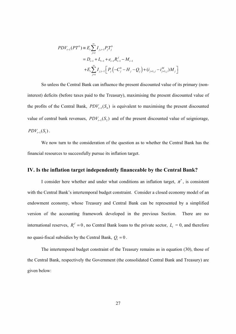
III. The intertemporal budget constraints of the Central Bank and the Treasury

17

To obtain a full understanding of the constraints the Central Bank is subject to in the

conduct of monetary policy in general and in its use of seigniorage in particular, it is essential to

have a view of the Central Bank as an economic agent with a period budget constraint and an

intertemporal budget constraint or solvency constraint. This requires us to decompose the

consolidated Government’s financial accounts and solvency constraint into separate accounts and

solvency constraints for the Central Bank and the Treasury (see also Buiter (2004), Sims (2004),

(2005) and Ize (2005)).6 In this Section, I therefore introduce a stylized set of accounts for a

small open economy. Separate period budget constraints for the Central Bank and Treasury are

also considered in Walsh (2003) and in Buiter (2003, 2004 and 2005). The latter also considers

the solvency constraints and intertemporal budget constraints of the two state sectors separately.

Walsh leaves out the payments made by the Central Bank to the Treasury. While this does not,

of course, affect the fiscal-financial-monetary options available to the consolidated Government,

it does prevent the consideration of how the Treasury can, through its fiscal claims on the Central

Bank, facilitate or prevent the Central Bank from implementing its monetary and supervisory

mandates.

The Central Bank has only the monetary base 0M ≥ on the liability side of its financial

balance sheet.7 The marginal cost of base money issuance is equal to zero. On the asset side it

has the stock of international foreign exchange reserves, fR , earning a risk-free nominal interest

rate in terms of foreign currency, fi , and the stock of domestic credit, which consists of Central

Bank holdings of nominal, interest-bearing Treasury bills, D , earning the risk-free domestic-

6 The term ‘government’ as used in ‘government budget constraint’ refers to the consolidated general government and central bank. ‘State’ would be a better term, to avoid confusion with the particular administration in office at a point in time. The unfortunate usage is, however, too firmly ensconced to try to dislodge it here. 7 In the real world this would be currency plus commercial bank reserves with the Central Bank. In many emerging markets and developing countries, the central bank also has non-monetary interest-bearing liabilities. These could be added easily to the accounting framework.

18

currency nominal interest rate, i , and Central Bank claims on the private sector, L , with risk-free

domestic-currency nominal interest rate Li ;8 e is the value of the spot nominal exchange rate (the

domestic currency price of foreign exchange); bT is the real value of taxes paid by the Central

Bank to the Treasury; it is a choice variable of the Treasury and can be positive or negative; H is

the real value of the transfer payments made by the Central Bank to the private sector (‘helicopter

drops’). I assume H to be a choice variable of the Central Bank. It is true that in most countries

the Central Bank is not a fiscal agent. I can neither tax nor make transfer payments. While I shall

deny the Central Bank the power to tax, 0H ≥ , I will until further notice allow it to make

transfer payments. This is necessary for ‘helicopter drops of money’ to be implementable by the

Central Bank on its own, without Treasury support; 0gC ≥ is real current consumption spending

by the Central Bank; the stock of Treasury debt (assumed to be denominated in domestic

currency) held outside the Central Bank is B ; it pays the risk-free nominal interest rate i ; pT is

the real value of the tax payments by the domestic private sector to the Treasury; it is a choice

variable of the Treasury and can be positive or negative; total real taxes net of transfer payments

received by the Government, that is, the consolidated Treasury and Central Bank are pT T H= − ;

0gC ≥ is the real value of Treasury spending on goods and services and 0bC ≥ the real value of

Central Bank spending on goods and services. Public spending on goods and services is assumed

to be public consumption only.

Equation (26) is the period budget identity of the Treasury and equation (27) that of the

Central Bank.

1 1, 1(1 )g p bt t t t

t t t t tt t

B D B DC T T iP P

− −−

+ −= − − − + (26)

8 For simplicity, I consider only short maturity bonds. Generalisations to longer maturities, index-linked debt or foreign-currency denominated debt are straightforward.

19

, 1 1 , 1 1 , 1 1 , 1 1(1 ) (1 ) (1 ) (1 )

fb bt t t t tt t t

tM L f ft t t t t t t t t t t t t

t

M D L e R C T HP

i M i D i L i e RP

− − − − − − − −

− − − = + +

+ − + − + − ++

(27)

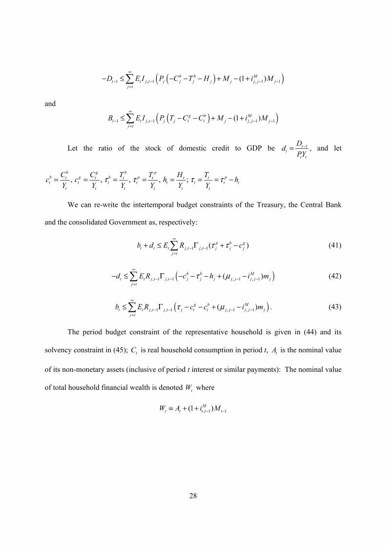
The solvency constraints of, respectively, the Treasury and Central Bank are given in equations

(28) and (29):

( ), 1lim 0t j t j jjE I B D−→∞

+ ≤ (28)

( ), 1lim 0ft j t j j j jj

E I D L e R−→∞+ + ≥ (29)

When there exist complete contingent claims markets, and the no-arbitrage condition is

satisfied, these solvency constraints, which rule out Ponzi finance by both the Treasury and the

Central Bank, imply the following intertemporal budget constraints for the Treasury (equation

(30)) and for the Central Bank (equation (31)).

1 1 , 1 ( )p b gt t t j t j j j j

j tB D E I P T T C

∞

− − −=

+ ≤ + −∑ (30)9

( ) ( )( )1 1 1 1 , 1 , 1 1(1 )f b b Mt t t t t j t j j j j j j j j j

j tD L e R E I P C T H Q M i M

∞

− − − − − − −=

+ + ≤ + + + − − +∑ (31)

where

, 1 , 1 1 , 1 , 1 1 11

( ) 1 (1 ) jL f fj j j j j j j j j j j j j

j

eP Q i i L i i e R

e− − − − − − −−

⎛ ⎞= − + + − +⎜ ⎟⎜ ⎟

⎝ ⎠ (32)

The expression Q in equation (32) stands for the real value of the quasi-fiscal implicit

interest subsidies made by the Central Bank. If the rate of return on government debt exceeds

that on loans to the private sector, there is an implicit subsidy to the private sector equal in period

t to ( ), 1 , 1 1L

t t t t ti i L− − −− . If the rate of return on foreign exchange reserves is less than what would be

9 Note that 1 , 1 1 , 1

, 1

11t t t t t t t

t t

E E I E Ii− − − −

−

= =+

.

20

implied by Uncovered Interest Parity (UIP), there is an implicit subsidy to the issuers of these

reserves, given in period t by , 1 , 1 1 11

1 (1 )f ftt t t t t t

t

ei i e Re− − − −

−

⎛ ⎞+ − +⎜ ⎟

⎝ ⎠.

The solvency constraint of the Central Bank only requires that the present

discounted value of its net non-monetary liabilities be non-positive in the long run. Its monetary

liabilities are liabilities only in name, as they are irredeemable: the holder of base money cannot

insist at any time on the redemption of a given amount of base money into anything else other

than the same amount of itself (base money).

Summing (26) and (27) gives the period budget identity of the consolidated Government

(the consolidated Treasury and Central Bank) in equation (33); summing (28) and (29) gives the

solvency constraint of the consolidated Government in equation (34) and summing (30) and (31)

gives the intertemporal budget constraint of the Government in equation (35).

, 1 1 , 1 1 , 1 1 , 1 1

( )

(1 ) (1 ) (1 ) (1 )

f g bt t t t t t t t t

M L f ft t t t t t t t t t t t t

M B L e R P C C T

i M i B i L e i R− − − − − − − −

+ − − ≡ + −

+ + + + − + − + (33)

( ), 1lim 0ft j t j j j jj

E I B L e R−→∞− − ≤ (34)

( )( )1 1 1 1 , 1 , 1 1(1 )f g b Mt t t t t j t j j j j j j j j j

j t

B L e R E I P T Q C C M i M∞

− − − − − − −=

− − ≤ − − − + − +∑ (35)

Consider the conventional financial balance sheet of the Central Bank in Table 1, that of

the Treasury in Table 2, and that of the Government in Table 3. Loans to the private sector and

international reserves are valued at their notional or face values.10

10 If the outstanding stock of loans to the private sector were marked-to-market, its fair value would be

1,

, 1

11

Lt t

tt t

iL

i+

+

⎛ ⎞+⎜ ⎟⎜ ⎟+⎝ ⎠

, the fair value of the international reserves would be. 1, 1

1,

(1 ) /ft t t tf

t tt t

i e ee R

i+ +

+

⎛ ⎞+⎜ ⎟⎜ ⎟⎝ ⎠

and the fair value of

21

Table 1 Central Bank Conventional Financial Balance Sheet Assets Liabilities

D

L

feR

M

bW

Table 2 Treasury Conventional Financial Balance Sheet Assets Liabilities

D

B

tW

the stock of base money would be 1,

1,

11

Mt t

tt t

iM

i+

+

⎛ ⎞+⎜ ⎟⎜ ⎟+⎝ ⎠

. As a store of value, base money is a perpetuity paying , 11 Mj ji −+

in each period j t> for each unit of money acquired in period t . The marked-to-market or fair value of a unit of base money acquired in period t (ex-dividend, that is, after period t interest due has been paid) is therefore

, 1 . 11

Mt j j j j

t

E I i∞

− −+∑ . In the deterministic case, this becomes , 1

1 1 , 11

Mjj j

j t k t k k

ii

∞−

= + = + −+∑ ∏ . If follows that, as a store of value,

the fair value of currency, which has a zero interest rate, is zero, as it is effectively a consol with a zero coupon.

22

Table 3 Government Conventional Financial Balance Sheet Assets Liabilities

L B

feR M

gW

The Central Bank’s financial net worth, b fW D L eR M≡ + + − , is the excess of the value

of its financial assets, Treasury debt, D , loans to the private sector, L and foreign exchange

reserves, feR , over its monetary liabilities, M . The Treasury’s conventional financial net worth

is denoted tW , the Government’s by gW .

To make the relationship between the intertemporal budget constraints of the Treasury

and the Central Bank and their conventional balance sheets more apparent, it is helpful to use the

ISI, given in equation (13), to rewrite the intertemporal budget constraint of the Central Bank as

in equation (36):

( ) ( )1 1 1 1 1 , 1 1, 1,( )f b b Mt t t t t t j t j j j j j j j j j j

j t

M D L e R E I P C T H Q i i M∞

− − − − − − + +=

⎡ ⎤− + + ≤ − − − − + −⎣ ⎦∑ (36)

III.1 Can Central Banks survive with ‘negative equity’?

On the left-hand side of (36) we have (minus) the equity of the Central Bank – the excess

of its monetary liabilities over its non-monetary financial assets. On the right-hand side of (36)

we have, in addition to the present discounted value of the Central Bank’s primary surpluses,

( ), 1b b

t j t j j j j jj t

E I P C T H Q∞

−=

− − − −∑ , the present discounted value Central Bank revenue,

23

, 1 1, 1,( )Mt j t j j j j j

j t

E I i i M∞

− + +=

−∑ , that is, the present discounted value of future interest payments saved

by the Central Bank because of its ability to issue monetary liabilities bearing an interest rate

, 1Mj ji − .

It should be noted that order to obtain the Central Bank’s intertemporal budget constraint

(31), I imposed the no-Ponzi game terminal condition ( ), 1lim 0ft j t j j j jj

E I D L e R−→∞+ + ≥ , that is, the

present value of the terminal net non-monetary liabilities had to be non-negative. I did not

impose the condition ( ), 1lim 0ft j t j j j j jj

E I D L e R M−→∞+ + − ≥ , that is, that the present value of the

terminal total net liabilities, monetary and non-monetary, had to be non-negative. To get from

(31) to (36), I need the ISI of equation (13), which is the basic ISI given in equation (11) plus the

terminal boundary condition (12), that is, ,lim 0t N t NNE I M

→∞= .

Although I will maintain condition (12) until Section V.2, it should be noted that, from

the point of view of the monetary authorities, this assumption is by no means obvious. The reason

is that the monetary ‘liabilities’ of the Central Bank are not in any meaningful sense liabilities of

the Central Bank. The owner (holder) of currency notes worth X units of currency have a claim

on the Central Bank for currency notes worth X units of currency – nothing more. The monetary

liabilities of the Central Bank are irredeemable or inconvertible into anything other than the same

amount of itself. While in most well-behaved economies, , 1lim 0t j t jjE I M−→∞

= , this will not be the

case, for instance, in a permanent liquidity trap where , 1lim lim 0t j t j t jj jE I M E M−→∞ →∞

= ≠ unless the

monetary authorities adopt a policy of (asymptotically) demonetising the economy in nominal

terms. Such asymptotic demonetization (in nominal terms) characterises the efficient stationary

liquidity trap equilibrium of the Bailey-Friedman Optimal Quantity of Money rule, when the

24

interest rate on base money is zero and the risk-free nominal interest rate on non-monetary assets

is kept at zero throughout. The nominal stock of base money shrinks at a proportional rate equal

to the real interest rate and the rate of time preference.

Even if the conventionally defined net worth or equity of the Central Bank is negative, that is, if

1 1 1 1 1 1 0b ft t t t t tW D L e R M− − − − − −≡ + + − < , the Central Bank can be solvent provided

( )1 , 1 1, 1,( )b b b Mt t j t j j j j j j j j j j

j t

W E I P C T H Q i i M∞

− − + +=

⎡ ⎤≥ + + + − −⎣ ⎦∑ . Conventionally defined financial net

worth or equity excludes the present value of anticipated or planned future non-contractual outlays and

revenues (the right-hand side of equation (36). It is therefore perfectly possible, for the central bank to

survive and thrive with negative financial net worth. This might, however, require the central bank to

raise so much seigniorage in real terms, , 1(1 )Mj j j j

j

M i MP

−− +, through current and future nominal base

money issuance, that, given the demand function for real base money, unacceptable rates of inflation

would result.

The financial net worth of the Treasury, ( )tW B D= − + is negative in most countries. The

financial net worth of the Government, that is, the consolidated Treasury and Central Bank

g t b fW W W eR L M B≡ + = + − − , is also negative for most countries. None of this need be a source

of concern, unless the gap between the outstanding contractual non-monetary debt of the state and the

present discounted value of the future primary (non-interest) surpluses of the state, g bj j j jT C C Q− − − ,

j t≥ is so large, that it either cannot be filled at all at all (the maximum value of the discounted future

real seigniorage stream is too low) and the state defaults, or can only be closed at unacceptably high rates

of inflation.

The only intertemporal budget constraint that ought to matter, that is, the only one that would

matter in a well-managed economy, is that of the consolidated Treasury and Central Bank, given in

25

equation (35). Its breakdown into the Treasury’s intertemporal budget constraint (equation (30)) and the

Central Bank’s intertemporal budget constraint (equation (31)) is without macroeconomic interest, unless

there is a failure of cooperation and coordination between the monetary and fiscal authorities, that is,

between the Central Bank and the Treasury. Operational independence for Central Banks may have raised

the risk of such mishaps occurring.

The separation of the accounts of the Treasury and the Central Bank allows us to

recognise a fourth measure of the revenues extracted by the state through its monopoly of the

issuance of base money. This is the conventionally measured operating profits of the Central

Bank (before payment of taxes to the Treasury), which will be denoted 4,tS . It consists of its net

interest income minus its operating expenses:

4, , 1 1 , 1 1 , 1 1 , 1 1L f f M b

t t t t t t t t t t t t t t t t t ti i e i P HS D L R i M PC− − − − − − − −+ −= + − − (37)

From equation (27) it follows that

4,f b

t t t t t t t tM D L e R PT S∆ − ∆ − ∆ − ∆ ≡ −

If we make the further assumption that the operating profits of the Central Bank are paid

in taxes to the Treasury11, that is,

4, ,bt t tP SΤ = (38)

then, and only then, does the textbook identity hold that the change in the stock of base money,

tM∆ , equals domestic credit expansion, t tD L∆ + ∆ , plus the value of the increase in the stock of

foreign exchange reserves, ft te R∆ :

ft t t t tM D L e R∆ = ∆ + ∆ + ∆ (39)

A little rearranging of the identities in (36) and (37) yields:

11 The profits of the Bank of England (after Corporation Tax) are split fifty-fifty between the Treasury and additions to the Bank of England’s reserves.

26

( )

, 1 4, 1 1 1 1 1

, 1

, 1 , 1 1 1 1 1 1

( )ft j t j t t t t t

j t

bt j t j j

j t

ft j t j j j j j j j

j t

E I S M D L e R

E I PT

E I i D L e R M

∞

− − − − − −=

∞

−=

∞

− − − − − − −=

≤ − + +

+

+ + + −

∑

∑

∑

(40)

So if the Treasury always taxes away all the operating profits of the Central Bank (equation (38)

holds), then

( )

( )

1 1 1 1 1 , 1 , 1 1 1 1 1

, 1 , 1 1 1

( )f ft t t t t t j t j j j j j j j

j t

ft j t j j j j j

j t

M D L e R E I i D L e R M

E I i e e R

∞

− − − − − − − − − − −=

∞

− − − −=

− + + ≤ + + −

+ −

∑

∑

From (39) it then follows that 1 1 1 1 1 1 for f fj j t j j j j j j jD L e R M D L e R M j t− − − − − −+ + − = + + − ≥ , so

( ), 1 , 1 1 1 0f

t j t j j j j jj t

E I i e e R∞

− − − −=

− ≥∑

So unless the Central Bank experiences, on average, capital gains (through currency

depreciation) rather than capital losses (through currency appreciation) on its foreign exchange

reserves, the Central Bank’s solvency constraint will be violated when the Treasury taxes away

its operating profits.

Regardless of the tax rule the Treasury imposes on the Central Bank, it is always the case

that the present discounted value of the taxes paid by Central Bank to the Treasury can be written

as

27

( )

1 , 1

1 1 1 1 1

, 1 1, 1,

( )

( )

b bt t j t j j

j t

ft t t t t

b Mt j t j j j j j j j j j

j t

PDV PT E I PT

D L e R M

E I P C H Q i i M

∞

− −=

− − − − −

∞

− + +=

≡

= + + −

⎡ ⎤+ − − − + −⎣ ⎦

∑

∑

So unless the Central Bank can influence the present discounted value of its primary (non-

interest) deficits (before taxes paid to the Treasury), maximising the present discounted value of

the profits of the Central Bank, 1 4( )tPDV S− is equivalent to maximising the present discounted

value of central bank revenues, 1 2( )tPDV S− and of the present discounted value of seigniorage,

1 1( )tPDV S− .

We now turn to the consideration of the question as to whether the Central Bank has the

financial resources to successfully pursue its inflation target.

IV. Is the inflation target independently financeable by the Central Bank? I consider here whether and under what conditions an inflation target, *π , is consistent

with the Central Bank’s intertemporal budget constraint. Consider a closed economy model of an

endowment economy, whose Treasury and Central Bank can be represented by a simplified

version of the accounting framework developed in the previous Section. There are no

international reserves, 0ftR = , no Central Bank loans to the private sector, tL = 0, and therefore

no quasi-fiscal subsidies by the Central Bank, 0tQ = .

The intertemporal budget constraint of the Treasury remains as in equation (30), those of

the Central Bank, respectively the Government (the consolidated Central Bank and Treasury) are

given below:

28

( )( )1 , 1 , 1 1(1 )b b Mt t j t j j j j j j j j

j tD E I P C T H M i M

∞

− − − −=

− ≤ − − − + − +∑

and

( )( )1 , 1 , 1 1(1 )g b Mt t j t j j t t j j j j

j tB E I P T C C M i M

∞

− − − −=

≤ − − + − +∑

Let the ratio of the stock of domestic credit to GDP be 1tt

t t

DdPY

−= , and let

, , , , ;b g b p

b g b p pt t t t t tt t t t t t t t

t t t t t t

C C T T H Tc c h hY Y Y Y Y Y

τ τ τ τ= = = = = = = −

We can re-write the intertemporal budget constraints of the Treasury, the Central Bank

and the consolidated Government as, respectively:

, 1 , 1( )p b gt t t j t j t j j j

j tb d E R cτ τ

∞

− −=

+ ≤ Γ + −∑ (41)

( ), 1 , 1 , 1 , 1( )b b Mt t j t j t j j j j j j j j

j td E R c h i mτ µ

∞

− − − −=

− ≤ Γ − − − + −∑ (42)

( ), 1 , 1 , 1 , 1( )g b Mt t j t j t j t t j j j j j

j tb E R c c i mτ µ

∞

− − − −=

≤ Γ − − + −∑ . (43)

The period budget constraint of the representative household is given in (44) and its

solvency constraint in (45); tC is real household consumption in period t, tA is the nominal value

of its non-monetary assets (inclusive of period t interest or similar payments): The nominal value

of total household financial wealth is denoted tW where

, 1 1(1 )Mt t t t tW A i M− −≡ + +

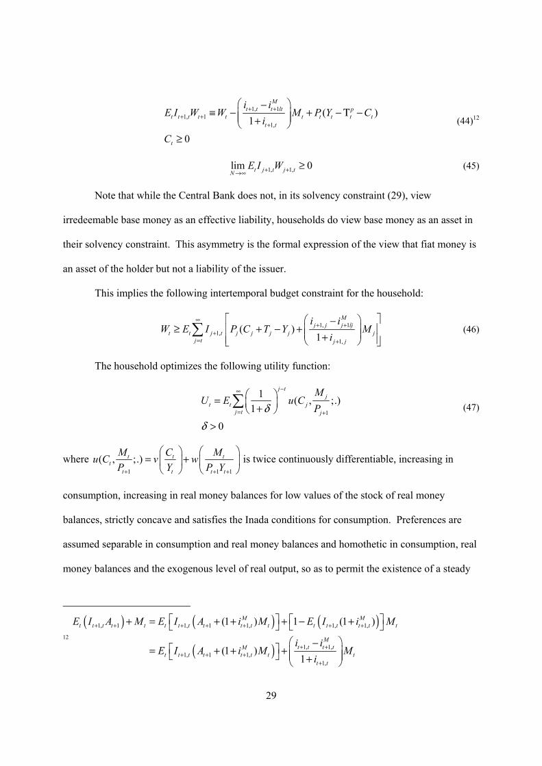
29

1, 1

1, 11,

( )1

0

Mt t t lt p

t t t t t t t t t tt t

t

i iE I W W M P Y C

i

C

+ ++ +

+

⎛ ⎞−≡ − + − Τ −⎜ ⎟⎜ ⎟+⎝ ⎠

≥

(44)12

1, 1,lim 0t j t j tNE I W+ +→∞

≥ (45)

Note that while the Central Bank does not, in its solvency constraint (29), view

irredeemable base money as an effective liability, households do view base money as an asset in

their solvency constraint. This asymmetry is the formal expression of the view that fiat money is

an asset of the holder but not a liability of the issuer.

This implies the following intertemporal budget constraint for the household:

1, 11,

1,

( )1

Mj j j lj

t t j t j j j j jj t j j

i iW E I P C T Y M

i

∞+ +

+= +

⎡ ⎤⎛ ⎞−≥ + − +⎢ ⎥⎜ ⎟⎜ ⎟+⎢ ⎥⎝ ⎠⎣ ⎦

∑ (46)

The household optimizes the following utility function:

1

1 ( , ;.)1

0

j tj

t t jj t j

MU E u C

Pδδ

−∞

= +

⎛ ⎞= ⎜ ⎟+⎝ ⎠

>

∑ (47)

where 1 1 1

( , ;.)t t tt

t t t t

M C Mu C v wP Y P Y+ + +

⎛ ⎞ ⎛ ⎞= +⎜ ⎟ ⎜ ⎟

⎝ ⎠ ⎝ ⎠ is twice continuously differentiable, increasing in

consumption, increasing in real money balances for low values of the stock of real money

balances, strictly concave and satisfies the Inada conditions for consumption. Preferences are

assumed separable in consumption and real money balances and homothetic in consumption, real

money balances and the exogenous level of real output, so as to permit the existence of a steady

12

( ) ( ) ( )

( )

1, 1 1, 1 1, 1, 1,

1, 1,1, 1 1,

1,

(1 ) 1 (1 )

(1 )1

M Mt t t t t t t t t t t t t t t t t t

Mt t t tM

t t t t t t t tt t

E I A M E I A i M E I i M

i iE I A i M M

i

+ + + + + + +

+ ++ + +

+

⎡ ⎤ ⎡ ⎤+ = + + + − +⎣ ⎦ ⎣ ⎦⎛ ⎞−⎡ ⎤= + + + ⎜ ⎟⎣ ⎦ ⎜ ⎟+⎝ ⎠

30

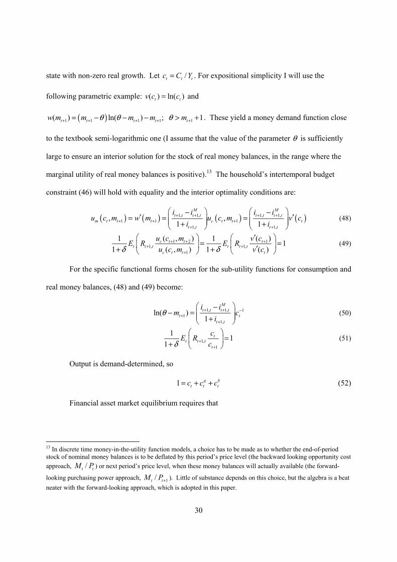
state with non-zero real growth. Let /t t tc C Y= . For expositional simplicity I will use the

following parametric example: ( ) ln( )t tv c c= and

( )1 1 1 1 1( ) ln( ) ; 1t t t t tw m m m m mθ θ θ+ + + + += − − − > + . These yield a money demand function close

to the textbook semi-logarithmic one (I assume that the value of the parameter θ is sufficiently

large to ensure an interior solution for the stock of real money balances, in the range where the

marginal utility of real money balances is positive).13 The household’s intertemporal budget

constraint (46) will hold with equality and the interior optimality conditions are:

( ) ( ) ( ) ( )1, 1, 1, 1,1 1 1

1, 1,

, ,1 1

M Mt t t t t t t t

m t t t c t t tt t t t

i i i iu c m w m u c m v c

i i+ + + +

+ + ++ +

⎛ ⎞ ⎛ ⎞− −′ ′= = =⎜ ⎟ ⎜ ⎟⎜ ⎟ ⎜ ⎟+ +⎝ ⎠ ⎝ ⎠

(48)

1 2 11, 1,

1

( , ) ( )1 1 11 ( , ) 1 ( )

c t t tt t t t t t

c t t t

u c m v cE R E Ru c m v cδ δ

+ + ++ +

+

⎛ ⎞ ⎛ ⎞′= =⎜ ⎟ ⎜ ⎟′+ +⎝ ⎠ ⎝ ⎠

(49)

For the specific functional forms chosen for the sub-utility functions for consumption and

real money balances, (48) and (49) become:

1, 1, 11

1,

ln( )1

Mt t t t

t tt t

i im c

iθ + + −

++

⎛ ⎞−− = ⎜ ⎟⎜ ⎟+⎝ ⎠

(50)

1,1

1 11

tt t t

t

cE Rcδ +

+

⎛ ⎞=⎜ ⎟+ ⎝ ⎠

(51)

Output is demand-determined, so

1 g bt t tc c c= + + (52)

Financial asset market equilibrium requires that

13 In discrete time money-in-the-utility function models, a choice has to be made as to whether the end-of-period stock of nominal money balances is to be deflated by this period’s price level (the backward looking opportunity cost approach, /t tM P ) or next period’s price level, when these money balances will actually available (the forward-

looking purchasing power approach, 1/t tM P+ ). Little of substance depends on this choice, but the algebra is a beat neater with the forward-looking approach, which is adopted in this paper.

31

t tA B= (53)14

Pricing behaviour is given by the slightly modified New-Keynesian Phillips curve in (54)

*

, 1 , 1 1 1 1, 1,1( ) ( )

10

t t t t t t t t t t t tE Y Y Eπ ω ϕ π ωδ

ϕ

− − − − + +− = − + −+

> (54)

Here * g bt t tY C C> + is the exogenously given level of capacity output or potential output. Its

proportional growth rate is denoted *

*, 1 *

1

1tt t

t

YY

γ −−

= − .

The Phillips curve in (54) combines Calvo’s model of staggered overlapping nominal

contracts (see Calvo (1983) and Woodford (2003)) with the assumption that even those price

setters who are free to set their prices have to do so one period in advance.15 The current price

level, tP is therefore predetermined. The variable , 1t tω − is the inflation rate chosen in period t-1

for period t by those price setters that follow a simple behavioural rule or heuristic. In the

original Calvo (1983) model, , 1 0t tω − = . I will assume that the period t inflation heuristic is the

future expected deterministic steady state rate of inflation of the model expected at time t-1:

, 1 1t t tEω π− −= (55)

Thus, while the price level in period t, tP , is predetermined, the rate of inflation in period

t, 1,t tπ + and in later periods in flexible. It is therefore possible to achieve an immediate transition

14 The household solvency constraint (45) and the consolidated Government solvency constraint government intertemporal budget constraint (34) (with 0f

jR = for the closed economy special case) together with t tA B= and

, 1 1(1 )Mt t t t tW A i M− −= + + imply that 1, 1 0t j t jE I M+ + ≥ , which, when holding with equality, was the assumption

made to obtain the version of the ISI given in (13). 15 Without the assumption that the optimising price setters have to set prices one period in advance, the Phillips curve

would be , 1 , 1 1, 1,1( ) ( )

1t t t t t t t t t t tY Y Eπ ω ϕ π ωδ− − + +− = − + −

+. Although prices would not be fully flexible,

unless , 1 , 1t t t tπ ω− −= for all t, there can be some response of the period t price level to events and news in period t.

32

to a different rate of inflation without any effect on real output, provided the change in monetary

policy is unexpected, immediate and permanent.

Economic decisions are made and equilibrium is established for periods 1t ≥ . Initial

financial asset stocks, 0 0,M D and 0 0 0, ,M B D are given. Central Bank instruments are , 1Mt ti − , th ,

btc and , 1t tµ − .16 Fiscal policy instruments are ,g b

t tc τ and ptτ .

It is clear that in the model developed here, as in any model with a predetermined price

level, Corollary 2 holds: maximising the present discounted value of current and future real

seigniorage is equivalent to maximising the present discounted value of future real Central Bank

revenues.

In the Neo-Keynesian model, the actual level of current output is demand-determined and

can therefore be influenced by past, present and anticipated future policy. In what follows I will

consider the deterministic special case of the model developed here. All exogenous variables and

policy instruments are constant. In period 0 the system starts off in a deterministic steady state.

Then, in period, 1t = , the monetary authorities announce a constant growth rate for the nominal

money stock, 1,t tµ µ+ = , which they will adhere to forever afterwards. If this growth rate for the

nominal money stock is different from the growth rate of the nominal money stock that supported

the original deterministic steady state, the announcement is unexpected but fully credible. For

this policy experiment to support an immediate transition to the new steady state, despite the

predetermined price level, the nominal money stock held at the end of period 1 (the beginning of

period 2) has to be set at the level that supports monetary equilibrium in period 1 with the new

steady-state stock of real money balances. This will, in general require a growth rate of the

16 It would be more descriptively realistic to make , 1t ti − a monetary policy instrument rather than , 1t tµ − . None of the results of this paper depend on this choice of monetary policy instrument and for expositional simplicity an exogenous growth rate of the nominal money stock is best here.

33

nominal money stock in period 1, 1,0µ that is different from the subsequent steady state growth

rate of the nominal money stock µ . This would certainly be the case if the demand for real

money balances in period t were to be defined in terms of /t tM P . It may also be required when

instead, as in the present paper, it is defined in terms of 1/t tM P+ .

The stationary equilibrium is characterised by the following conditions for 1t ≥ :

1 g btc c c= − − (56)

equilibrium: 1,t tr ρ+ = (57)

1, *

111t t

µπγ+

++ =+

(58)

1, 1,1 (1 )(1 )t t t ti ρ π+ ++ = + + (59)

( )

1, 1

1,

1,1

1,

11

( )1

orM

t tt

t t

Mt t

t tt t

i ic

it

i iv m v c

i

m eθ+ −

+

++

+

⎛ ⎞−⎜ ⎟⎜ ⎟+⎝ ⎠

+

⎛ ⎞−′ ′= ⎜ ⎟⎜ ⎟+⎝ ⎠

= −

(60)

*t tY Y= (61)

1, 1,t t t tω π π+ += = (62)

I am only considering equilibria where Mi i≥ and *ρ γ> .

I want to consider which constant rate(s) of inflation, π π= , this economy can support,

with a Central Bank whose intertemporal budget constraint is given by equation (42). With the

economy in steady state from period 1, it follows that the Central Bank’s intertemporal budget

constraint can be rewritten as follows:

( ) ( )* *

1* *

1 1 ( )b b Mtd c h i mγ γτ µ σ π

ρ γ ρ γ⎛ ⎞ ⎛ ⎞+ +− + + + ≤ − =⎜ ⎟ ⎜ ⎟− −⎝ ⎠ ⎝ ⎠

(63)

34

where

2

'( ) 1 ''( )( ; , , ); 0; 0''( ) 1 )(1 ) 1 ''( )

M MM

cv c i i i v cm c i

w m i w mππ ρρ π

⎛ ⎞ ⎛ ⎞+ −= = < = >⎜ ⎟ ⎜ ⎟( + + +⎝ ⎠ ⎝ ⎠l l l (64)

For the specific functional form (1 )(1 ) (1 )

(1 )(1 )

Micm e

ρ πρ πθ

⎛ ⎞+ + − +⎜ ⎟⎜ ⎟+ +⎝ ⎠= − , we have

( )( )*

* *1* 2

1 1(1 ) (1 )(1 ) (1 )(1 )(1 )

MMd im i m

d cσ γ γ π γ θπ ρ γ ρ π

⎡ ⎤⎛ ⎞ ⎛ ⎞+ += + − + + − + −⎢ ⎥⎜ ⎟ ⎜ ⎟− + +⎝ ⎠ ⎝ ⎠⎣ ⎦

Consider the case where the nominal interest rate on base money is zero, so

(1 )(1 ) 1 (1 )(1 ) 1* *(1 )(1 ) (1 )(1 )*1

* 2

1 (1 )(1 ) 1(1 )(1 )(1 )

c cd e ed c

ρ π ρ πρ π ρ πσ γ π γγ θ

π ρ γ ρ π

⎛ ⎞ ⎛ ⎞+ + − + + −⎜ ⎟ ⎜ ⎟+ + + +⎝ ⎠ ⎝ ⎠

⎡ ⎤⎛ ⎞⎛ ⎞ ⎛ ⎞+ + + −⎢ ⎥⎜ ⎟= + − −⎜ ⎟ ⎜ ⎟⎜ ⎟− + +⎢ ⎥⎝ ⎠ ⎝ ⎠⎝ ⎠⎣ ⎦ (65)

Assume both the long-run nominal interest rate and the long-run growth rate of nominal

GDP are non-negative. Then 1 0ddσπ

> when 0π = provided the demand for real money balances

is sufficiently large at a zero rate of inflation. A sufficiently large value of 1 b gc c c= − + , steady

state consumption as a share of GDP, will ensure that. I assume this condition is satisfied. The

long-run seigniorage Laffer curve has a single peak at

( )

( ) ( )*

11 2 * *

1 1

ˆ(1 )(1 ) (1 ) (1 )ˆ

ˆ ˆ(1 )(1 ) (1 ) (1 )(1 ) (1 ) (1 )

M M

M M

i im m

c i i

π γ θρ π γ π γ

+ + − + += =

+ + + + + + − + +

where 1 1ˆ arg maxπ σ=

Let minbπ be the lowest constant inflation rate that is consistent with the Central Bank’s

intertemporal budget constraint, given in (63), for given values of , 0,b btd c τ≥ and 0h ≥ .17 If there is

a long-run Seigniorage Laffer curve, minbπ may not exist: there may be no constant inflation rate that

17 That is, minbπ is the lowest value of π that solves ( )

*

1*

1 ( )b btd c hγ τ σ π

ρ γ⎛ ⎞+− + + + =⎜ ⎟−⎝ ⎠

.

35

would generate enough real seigniorage to satisfy (63). If the value of the inflation target, *π , is less than

minbπ , then the Central Bank cannot achieve the inflation target, because doing so would bankrupt it. The

most it could do would be to set both bc and h equal to zero: there would be no Central Bank-initiated

helicopter drops of money and Central Bank staff would not get paid. If that is not enough to cause the

weak inequality in (63) to be satisfied with *π π π= = , I will call this a situation where the inflation

target is not independently financeable by the Central Bank. The value of the Central Bank’s holdings of

Treasury debt, td , is determined by history; the net tax paid by the Central Bank to the Treasury, bτ is

determined unilaterally by the Treasury. I summarise this as follows:

Proposition 3:

If either minbπ does not exist or *

minbπ π< , the inflation target is not independently

financeable by the Central Bank.

If the Treasury decides to support the Central Bank in the pursuit of the inflation

objective, the inflation target is jointly financeable by the Central Bank and the Treasury, as long

as the consolidated intertemporal budget constraint of the Treasury and the Central Bank can be

satisfied with the seigniorage revenue generated by the implementation of the inflation target.

The intertemporal budget constraint of the Treasury and of the consolidated Government for this

simple economy are given by, respectively:

( )*

*

1 p b gt tb d cγ τ τ

ρ γ⎛ ⎞++ ≤ + −⎜ ⎟−⎝ ⎠

(66)

( )*

1*

1 ( )g btb c cγ τ σ π

ρ γ⎛ ⎞++ + − ≤⎜ ⎟−⎝ ⎠

(67)

Let mingπ be the lowest constant inflation rate that is consistent with the intertemporal

budget constraint of the consolidated Government, given in (67), for given values of

36

, 0, 0g btb c c≥ ≥ and τ . Again, min

gπ could either not exist or could exceed the inflation target

*π . This suggests the following:

Proposition 4:

If either mingπ does not exist or if *

mingπ π< , the inflation target is not financeable, even

with cooperation between Treasury and Central Bank. The inflation target in that case is not feasible.

If (67) is satisfied with *π π= , the inflation target is financeable by the consolidated

Treasury and Central Bank – that is, the inflation target is feasible with cooperation between

Treasury and Central Bank. It may of course (if (63) is satisfied as well as (67)), also be

independently financeable by the Central Bank. Note that the feasibility condition for the

inflation target, equation (67), is independent of bτ (which is a transfer payment within the

consolidated Treasury and Central Bank) and of td which is an internal liability/asset within the

consolidated Treasury and Central Bank. What matters is the net debt of the consolidated

Treasury and Central Bank, tb , and the taxes net of transfers of the consolidated Treasury and

Central Bank, τ . If the feasibility condition (67) is satisfied, the Treasury can always provide

the Central Bank with the resources it requires to implement the inflation target. All it has to do

is reduce taxes on the Central Bank (or increase transfer payments to the Central Bank), in an

amount sufficient to ensure that equation (63) is also satisfied.18

If (67) is satisfied with *π π= , but (63) is not, then the inflation target is only financeable

by the Treasury and Central Bank jointly, not independently by the Central Bank. Note that this

can only happen if the Treasury has ‘surplus’ resources, that is, (66) holds as a strict inequality.

In that case, a reduction in bτ can permit the Central Bank’s intertemporal budget constraint (63)

18 This could be achieved through a one-off capital transfer rather than through a sequence of current transfers.

37

to be satisfied without violating the Treasury’s intertemporal budget constraint (67). I summarise

this as follows:

Proposition 5:

If *min minb gπ π π< < , the inflation target is only cooperatively financeable by the Central

Bank and the Treasury jointly.

This discussion provides an argument in support of the view that the Central Bank should

not have operational target independence (freedom to choose a quantitative inflation target) even

when it has operational independence (the freedom to set the monetary instrument (typically a

short nominal interest rate, but in this paper the growth rate of the nominal stock of base money,

as it sees fit). The reason is that if the political authorities choose the operational target, there is

less of a risk of ‘mandating without funding’. On its own, the Central Bank cannot be guaranteed

to have the right degree of financial independence. Without Treasury support, there can be no

guarantee that the minimal amount of seigniorage required to ensure the solvency of the Central

Bank can support the inflation target. If *min minb gπ π π< < , only the Treasury can make sure that the

Central Bank has enough resources to make the inflation target financeable by the Central Bank.

The Treasury, through its ability to tax the Central Bank, is effectively constrained only by the

consolidated intertemporal budget constrained in (67), even though formally it faces the

intertemporal budget constraint given in equation (66).

V. Other aspects of necessary co-operation and co-ordination between Central Bank and Treasury

Even if the Treasury supports the Central Bank’s inflation target and provides it with the

financial resources to implement it, there are at least two other economic contingencies for which

active Central Bank and Treasury co-ordination and co-operation is desirable.

38

V.1 Recapitalizing the central bank

The first case occurs when the (threat of) a serious banking crisis or financial crisis with

systemic implications forces the Central Bank to act as a lender of last resort, and the problem

turns out to be (or becomes), for a significant portion of the banking/financial system, a solvency

crisis as well as a liquidity crisis. It could happen that recapitalising the insolvent banks or

financial institutions with only the financial resources of the Central Bank (including a given

sequence of net payments to the treasury, bT ) would require the Central Bank to engage in

excessive base money issuance, which would result in unacceptable rates of inflation. As long as

the resources of the consolidated Treasury and Central Bank are sufficient, the Treasury could

either recapitalise the Central Bank (if the Central Bank recapitalised the private

banking/financial system in the first instance), or the Treasury could directly recapitalise the

banking/financial system. In the accounts set out above, recapitalising the Central Bank would

amount to one or more large negative realisations of bT , with as counterparts an increase in

Central Bank holdings of Treasury debt, D (see Ize (2005)).

Special problems occur when the insolvency of (part of) the financial system is due to an

excess of foreign-currency liabilities over foreign-currency assets. In that case the Treasury, in

order to recapitalise the Central Bank (or some other part of the financial sector directly), has to

be able to engineer both an internal fiscal transfer and an external transfer of resources of the

required magnitude. If the external credit of the state is undermined, this may only be possible

gradually, if and as the state can lay claim to (part of) the current and future external primary

surpluses of the nation.

In the usual nation state setting, a single Treasury or national fiscal authority stands behind

a single central bank. Unique complications arise in the EMU, where each national fiscal

39

authority stands financially behind its own national central bank (NCB), but no fiscal authority

stands directly behind the ECB. The lender of last resort function in the EMU is assigned to the

NCB members of the ESCB (see Padoa-Schioppa (2004) and Goodhart (2002)). This will work

fine when a troubled or failing bank or other financial institution deemed to be of systemic

importance has a clear nationality, as most Eurozone-domiciled banks and other financial

institutions do today. Likewise, banks that are subsidiaries of institutions domiciled outside the

EMU will be the responsibility of their respective national Central Banks and of the national

fiscal authority that stands behind each of these Central Banks.

Trouble arises as and when Eurozone-domiciled banks emerge that do not have a clear

national identity, say banks incorporated solely under European Law. As there is no fiscal

authority, national or supranational, standing behind the ECB, who would organise and fund the

bail-out and recapitalisation of such a ‘European bank’? Whether this potential vulnerability will

in due course be remedied by the creation of a serious supra-national fiscal authority at the EMU

level that would stand behind the ECB, or by implicit or explicit agreements between the ECB,

the NCBs (the shareholders of the ECB) and the national fiscal authorities is as yet unclear.

V.2 Helicopter drops of money

The second set of circumstances when cooperation and coordination between the monetary

and fiscal authorities is essential is when an economy is confronting the need to avoid unwanted

deflation or, having succumbed to it, to escape from it. In principle, the potential benefits from

cooperation between the monetary and fiscal authority apply to stabilisation policy in general,

that is to counter-inflationary as well as to counter-deflationary policies. The issue is particularly

40

urgent, however, when deflation is the enemy and conventional monetary policy has run out of

steam.

Faced with deflation, the Central Bank on its own can cut the short nominal interest rate -

the primary monetary policy instrument in most economies with a floating exchange rate. It can

engage in sterilised foreign exchange market operations. If there are reserve requirements

imposed on commercial banks or other financial institutions, these can be relaxed, as can the

collateral standards in Repos and the eligibility requirements that must be met by potential

counterparties.

Once the short nominal interest rate is at the zero floor, conventional monetary policy is

effectively exhausted. The Central Bank can then engage in generalised open market purchases,

monetising the outstanding stock of non-monetary public debt, of all maturities, nominally

denominated or index-linked, held outside the Central Bank. Once all outstanding public debt

has been absorbed by the Central Bank, it could turn its attention to the purchase and

monetisation of private securities, from foreign currency-denominated securities, to stocks and

shares, land, property or contingent claims. Clearly, such socialisation of private wealth would

be subject to all kinds of moral hazard, adverse selection and governance problems.

Should this too fail to boost aggregate demand and end deflation, the monetary authority on

its own has one remaining exotic instrument and the combined monetary and fiscal authorities

have one conventional but truly effective instrument. The unconventional instrument is to lower

the zero floor on nominal interest rates (which is a result of the zero nominal interest rate paid on

currency and often on all base money), by paying a negative nominal interest rate on base money.

For commercial banks’ reserves with the central bank, paying a negative nominal interest rate is

technically and administratively trivial. Imposing a ‘carry tax’ on currency (setting a negative

41

value for Mi ) is administratively cumbersome and intrusive, but not impossible. Silvio Gesell

(1916) recommended it many years ago, and as great an economist as Irving Fisher (1933)

thought the proposal had merit (see also Goodfriend (2000) and Buiter and Panigirtzoglou (2001,

2003)).

There is, however, a very conventional policy alternative. Milton Friedman referred to it

as (base) money dropped from a helicopter (Friedman (1968)). If the recipients of this largesse

do not expect it to reversed (in present discounted value terms) in the future, this would, at a

given price level, represent an increase in the real net wealth of the private sector (see Buiter

(2003)). Because base money does not have to be redeemed ever, it does not constitute an

effective liability of the state. The increase in net private wealth is also in the most liquid form

possible.19

An example of a helicopter drop, in the UK context, would be for the Governor of the

Bank of England issue a £1,000 cheque, drawn upon the Bank of England, to every man, woman

and child in the country. On the balance sheet of the Bank this would show up as an increase in

the stock of base money and a corresponding reduction in the financial net worth of the Bank. In

its budget constraint it would be a one-off transfer payment to the private sector (h in our

notation).

Would it work? If the money rain is not expected to be reversed in present value, it surely

would. It does not rely on the strength of the intertemporal substitution effect in private

consumption or on the interest sensitivity of private investment demand. All that it requires is

that aggregate consumption today is a normal good. If the wealth effect is weak and the

19 In this case, the boundary condition 1, 1 0t j t jE I M+ + ≥ would hold as a strict inequality.

42

£1,000.00 cheque does not do the job, the Governor can add zeros in front of the decimal point

on the cheque until the private consumer surrenders and goes out and spends.

Even if the economic mechanism of the helicopter drop of money is straightforward, its

practical implementation cannot be done by the Central Bank alone. The reason is that in reality

central banks do not have an instrument like H in their arsenals. Making transfer payments to the

private sector is not something Central Banks are legally permitted to do, because they are not

fiscal agents of the state. So the economically equivalent action has to be coordinated between

the Treasury and the Central Bank. The treasury will implement a tax cut or increase in transfer

payments (a cut in pT ) and will finance this by selling debt to the Central Bank (increasing D).

The acquisition of Treasury debt by the central bank is financed through the issuance of base

money, an increase in M.

VI. Conclusion

Governments through the ages have appropriated real resources through the monopoly of

the ‘coinage’. In modern fiat money economies, the monopoly of the issue of legal tender is

generally assigned to an agency of the state, the Central Bank, which may have varying degrees

of operational and target independence from the government of the day.

In this paper I analyse four different but related concepts, each of which highlights some

aspect of the way in which the state acquires command over real resources through its ability to

issue fiat money. They are (1) seigniorage (the change in the monetary base), (2) Central Bank

revenue (the interest bill saved by the authorities on the outstanding stock of base money

liabilities), (3) the inflation tax (the reduction in the real value of the stock of base money due to

43

inflation and (4) the operating profits of the central bank, or the taxes paid by the Central Bank to

the Treasury.

To understand the relationship between these four concepts, an explicitly intertemporal

approach is required, which focuses on the present discounted value of the current and future

resource transfers between the private sector and the state. Furthermore, when the Central Bank

is operationally independent, it is essential to decompose the familiar consolidated ‘government

budget constraint’ and consolidated ‘government intertemporal budget constraint’ into the

separate accounts and budget constraints of the Central Bank and the Treasury. Only by doing

this can we appreciate the financial constraints on the Central Bank’s ability to pursue and

achieve an inflation target, and the importance of cooperation and coordination between the

Treasury and the Central Bank when faced with financial sector crises involving the need for

long-term recapitalisation or when confronted with the need to mimick Milton Friedman’s

helicopter drop of money in an economy faced with a liquidity trap.

44

References

Anand, Ritu and Sweder van Wijnbergen (1989), “Inflation and the Financing of Government Expenditure: an Introductory Analysis with an Application to Turkey”, World Bank Economic Review, Vol. 3, No. 1, pp. 17-38. Blinder, Alan S. and Robert M. Solow (1973), “Does fiscal policy matter?”, Journal of Public Economics, 2, pp. 319-337. Bordo, Michael (2006), “Comment on Marc Flandreau, ‘Pillars of Globalization: A History of Monetary Policy Targets, 1797-1997’”, Prepared for the Fourth ECB, Monetary Policy conference, Frankfurt November 9-10 2006. http://www.ecb.int/events/pdf/conferences/cbc4/Discussion_Bordo.pdf Bresciani-Turroni, Constantino (1937), The Economics of Inflation: A Study of Currency Depreciation in Post-War Germany. London, Allen and Unwin. Buiter Willem H. (1990), Principles of Budgetary and Financial Theory, MIT Press, Cambridge, Massachusetts.

Buiter, Willem H. (2003), "Helicopter Money: Irredeemable Fiat Money and the Liquidity Trap", NBER Working Paper No. W10163, December .

Buiter, Willem H. (2004), “Two naked emperors? Concerns about the Stability and Growth Pact and second thoughts about Central Bank independence”, Fiscal Studies, Vol. 25(3), pp. 249-77.

Buiter, Willem H. (2005), "New Developments in Monetary Economics: two ghosts, two eccentricities, a fallacy, a mirage and a mythos", Royal Economic Society 2004 Hahn Lecture, The Economic Journal, Conference Papers, Vol. 115, No. 502, March 2005, pp. C1-C31.

Buiter, Willem H. and Nikolaos Panigirtzoglou (2001), "Liquidity Traps: How to Avoid Them and How to Escape Them", with Nikolaos Panigirtzoglou, in Reflections on Economics and Econometrics, Essays in Honour of Martin Fase, edited by Wim F.V. Vanthoor and Joke Mooij, 2001, pp. 13-58, De Nederlandsche Bank NV, Amsterdam.

Buiter, Willem H. and Nikolaos Panigirtzoglou (2003), "Overcoming the Zero Bound on Nominal Interest Rates with Negative Interest on Currency: Gesell’s Solution", Economic Journal, Volume 113, Issue 490, October 2003, pp. 723-746.

Cagan, Philip (1956), "Monetary Dynamics of Hyperinflation", in Milton Friedman, Editor, Studies in the Quantity Theory of Money, University of Chicago Press, Chicago, Illinois. Calvo, Guillermo (1983), ”Staggered Contracts in a Utility-Maximizing Framework”, Journal of Monetary Economics, September.

45

Christ, Carl (1968), "A Simple Macroeconomic Model with a Government Budget Restraint," Journal of Political Economy 76, No. 1, January/February, pp. 53-67. Dornbusch, Rudiger, and Staley Fischer (1986), “Stopping Hyperinflations Past and Present”, Weltwirtschaftliches Archiv 122, pp. 1-47. Easterly, William R., Paolo Mauro, Klaus Schmidt-Hebbel (1995), “Money Demand and Seigniorage-Maximizing Inflation”, Journal of Money, Credit and Banking, Vol. 27, No. 2 (May), pp. 583-603. Fisher, Irving (1933), Stamp Scrip, Adelphi Company, New York. Flandreau, Marc (2006), “Pillars of Globalization: A history of monetary policy targets, 1797-1997”, Revised Draft : November 2, 2006, Paper prepared for the Fourth ECB Central Banking Conference, Frankfurt-Am-Main, November 9-10 2006. http://www.ecb.int/events/pdf/conferences/cbc4/Flandreau.pdf

Friedman, Milton (1968), "The Role of Monetary Policy." American Economic Review 58, no. 1, pp. 1-17.

Friedman, M.(1971), “Government Revenue from inflation”, Journal of Political Economy, vol. 79, N° 4, pp. 846-56. Gesell, Silvio (1916, 1949), Die Natuerliche Wirtschaftsordnung, Rudolf Zitzman Verlag, available in English as The Natural Economic Order, Peter Owen Ltd, London, 1958. Goodfriend, Marvin (2000), “Overcoming the Zero Bound on Interest Rate Policy, Journal of Money, Credit and Banking, Vol. 32, No. 4, Pt. 2, November, pp. 1007-1035. Goodhart, Charles (2002), “Recent Developments in Central Banking.” In Monetary Policy, Capital Flows and Exchange Rates: Essays in Honour of Maxwell Fry. Edited by Fry, M. J.; Dickinson, D. G.; Allen, B. Routledge, Ize, Alain (2005), “Capitalising Central Banks: A Net Worth Approach”, IMF Working Paper,

WP/05/15 January 2005 Kiguel, Miguel A. and Pablo A. Neumeyer (1995), “Seigniorage and Inflation: The Case of Argentina”, Journal of Money, Credit and Banking, Vol. 27, No. 3 (Aug.), pp. 672-682. King, Robert G. and C. I. Plossser (1985), “Money, Deficits and Inflation”, Carnegie-Rochester Conference Series on Public Policy, 22, Spring, pp. 147-196. Padoa-Schioppa, Tommaso (2004). The Euro and Its Central Bank, The MIT Press, Cambridge, Massachusetts.

46

Phelps, , Edmund (1973), Inflation in the Theory of Public Finance”, Swedish Journal of Economics, 75, March, pp. 67-82. Romer, David (2006), Advanced Macroeconomics, Third Edition, Chapter 10. McGraw-Hill, New York. Sargent, Thomas J. (1982), “The End of Four Big Inflations”, in Robert E. Hall, ed., Inflation, pp. 41-98, University of Chicago Press, Chicago Illinois. Sargent, Thomas J. (1987), Dynamic Macroeconomic Theory, Harvard University Press, Cambridge, Massachusetts. Sargent, Thomas J. and Neil Wallace (1981), “Some unpleasant monetarist arithmetic”, Federal Reserve Bank of Minneapolis Quarterly Review, 5(3), pp. 1-17. Sims, C. A. (2004): “Fiscal Aspects of Central Bank Independence,” Chapter 4, p.103-116, in European Monetary Integration, Hans-Werner Sinn, Mika Widgrén, and Marko Köthenbürger, editors, MIT Press. Sims, C. A. (2005), “Limits to Inflation Targeting”, Chapter 7 in The Inflation-Targeting Debate, Ben S. Bernanke and Michael Woodford, editors, NBER Studies in Business Cycles Volume32, p. 283-310. Thornton, H. (1802), An Enquiry into the Nature and Effects of the Paper Credit of Great Britain. Tobin, James and Willem H. Buiter (1976), “ Long-run effects of fiscal and monetary policy on aggregate demand”, in J. Stein ed. Monetarism, North Holland, Amsterdam, pp. 273-309. Walsh, Carl E. (2003), Monetary Theory and Policy, 2nd Edition, Chapter 4, pp. 135-197, The MIT Press, Cambridge Massachusetts. Woodford, Michael (2003), Interest & Prices; Foundations of a Theory of Monetary Policy, Princeton University Press, Princeton and Oxford.

CENTRE FOR ECONOMIC PERFORMANCE Recent Discussion Papers

785 Gustavo Crespi Chiara Criscuolo Jonathan E. Haskel Matthew Slaughter

Productivity Growth, Knowledge Flows and Spillovers

784 Richard Layard Guy Mayraz Stephen Nickell

The Marginal Utility of Income

783 Gustavo Crespi Chiara Criscuolo Jonathan E. Haskel

Information Technology, Organisational Change and Productivity Growth: Evidence from UK Firms

782 Paul Castillo Carlos Montoro Vicente Tuesta

Inflation Premium and Oil Price Volatility

781 David Metcalf Why Has the British National Minimum Wage Had Little or No Impact on Employment?

780 Carlos Montoro Monetary Policy Committees and Interest Rate Smoothing

779 Sharon Belenzon Mark Schankerman

Harnessing Success: Determinants of University Technology Licensing Performance

778 Henry G. Overman Diego Puga Matthew A. Turner

Decomposing the Growth in Residential Land in the United States

777 Florence Kondylis Conflict-Induced Displacement and Labour Market Outcomes: Evidence from Post-War Bosnia and Herzegovina

776 Willem H. Buiter Is Numérairology the Future of Monetary Economics? Unbundling numéraire and medium of exchange through a virtual currency and a shadow exchange rate

775 Francesco Caselli Nicola Gennaioli

Economics and Politics of Alternative Institutional Reforms

774 Paul Willman Alex Bryson

Union Organization in Great Britain Prepared for symposium for the Journal of Labor Research on “The State of Unions: A Global Perspective”

773 Alan Manning The Plant Size-Effect: Agglomeration and Monopsony in Labour Markets

772 Guy Michaels The Effect of Trade on the Demand for Skill – Evidence from the Interstate Highway System

771 Gianluca Benigno Christoph Thoenissen

Consumption and Real Exchange Rates with Incomplete Markets and Non-Traded Goods

770 Michael Smart Daniel M. Sturm

Term Limits and Electoral Accountability

769 Andrew B. Bernard Stephen J. Redding Peter K. Schott

Multi-Product Firms and Trade Liberalization

768 Paul Willman Alex Bryson

Accounting for Collective Action: Resource Acquisition and Mobilization in British Unions

767 Anthony J. Venables Shifts in Economic Geography and their Causes

766 Guy Michaels The Long-Term Consequences of Regional Specialization

765 Fabrice Murtin American Economic Development Since the Civil War or the Virtue of Education

764 Carlo Rosa Giovanni Verga

The Impact of Central Bank Announcements on Asset Prices in Real Time: Testing the Efficiency of the Euribor Futures Market

763 Benjamin Aleman-Castilla

The Effect of Trade Liberalization on Informality and Wages: Evidence from Mexico

762 L. Rachel Ngai Roberto M. Samaniego

An R&D-Based Model of Multi-Sector Growth

761 Mariano Bosch Job Creation and Job Destruction in the Presence of Informal Labour Markets

760 Christian Hilber Frédéric Robert-Nicoud

Owners of Developed Land Versus Owners of Undeveloped Land: Why Land Use is More Constrained in the Bay Area than in Pittsburgh

759 William Nickell The CEP-OECD Institutions Data Set (1060-2004)

758 Jean Eid Henry G. Overman Diego Puga Matthew Turner

Fat City: the Relationship Between Urban Sprawl and Obesity

The Centre for Economic Performance Publications Unit Tel 020 7955 7673 Fax 020 7955 7595 Email info@cep.lse.ac.uk

Web site http://cep.lse.ac.uk