ISSN 2042-2695

CEP Discussion Paper No 1533

April 2018

Changing the Structure of Minimum Wages: Firm Adjustment and Wage Spillovers

Giulia Giupponi Stephen Machin

Abstract This paper analyses the economic impact of a significant change to the structure of a minimum wage setting policy. The context is the United Kingdom where government mandated an unexpected change in the structure of minimum wages and their setting in 2016 by introducing a new minimum wage – the National Living Wage (NLW) – for workers aged 25 and over. The new NLW rate was significantly higher than the minimum wage for those under age 25. The analysis studies the consequences of this change in a sector containing many low wage workers, the care homes industry. The new minimum wage structure and associated higher minimum wage for those aged 25 and above significantly affected wages, but at the same time with little evidence of adverse employment effects, nor firm closure. Rather the margin of adjustment used to offset the sizable wage cost shock was a significant deterioration of the quality of care services. There is also strong evidence of wage spillovers as younger workers wages rose in tandem with the higher adult minimum wage, but with no impact on their employment. Based on further empirical tests, employer preference for fairness seems to offer the most plausible explanation for these results. Key words: minimum wage structure, employment, wage spillovers JEL: J23; J31 This paper was produced as part of the Centre’s Labour Markets Programme. The Centre for Economic Performance is financed by the Economic and Social Research Council. We would like to thank Attila Lindner, Alan Manning, Steve Pischke and participants in seminars at the London School of Economics, the Low Pay Commission, the Labour Institute for Economic Research in Helsinki and the 2018 Royal Economic Society Annual Conference for comments and suggestions. We are also grateful to Roy Price of Skills for Care for helpful assistance with the NMDS-SC data and to Nigel Rogers for assistance with survey management. We acknowledge financial support in the initial par t of this work undertaken with Attila Lindner and Alan Manning for the Low Pay Commission. Giulia Giupponi, Department of Economics and Centre for Economic Performance, London School of Economics. Stephen Machin, Department of Economics and Centre for Economic Performance, London School of Economics. Published by Centre for Economic Performance London School of Economics and Political Science Houghton Street London WC2A 2AE All rights reserved. No part of this publication may be reproduced, stored in a retrieval system or transmitted in any form or by any means without the prior permission in writing of the publisher nor be issued to the public or circulated in any form other than that in which it is published. Requests for permission to reproduce any article or part of the Working Paper should be sent to the editor at the above address. G. Giupponi and S. Machin, submitted 2018.

1

1. Introduction

The by now centennial history of minimum wages and their widespread application across

developed and developing countries has triggered a great deal of academic research on the topic.

Recent years have seen a burst of renewed interest in this topic in both academic and policy settings

around the world. In this paper, we study what happened to a range of economic outcomes when

there was a substantive recent change in the structure of a minimum wage setting policy. This

occurred in the UK when a government that had traditionally been hostile to minimum wages

introduced an unexpected and sizable increase for older workers by introducing a new minimum

wage rate – the National Living Wage (NLW). This new minimum wage rate for workers aged 25

and over moved the number of minimum wages in operation in the UK labour market up from four

to five and, in doing so, structurally altered the minimum wage policy in operation in the labour

market.

We are interested in analysing the consequences of this change in the UK minimum wage

structure on three big areas of research that have been traditionally explored in the minimum wage

literature. Firstly, wage and employment effects are studied in the context of workers and firms in

the UK care homes sector, which has been argued to be a good testing ground for evaluating

minimum wage effects on employment in earlier research (Machin, Manning and Rahman, 2003;

Machin and Wilson, 2004). Secondly, we exploit the change in minimum wage structure to study

whether the UK National Living Wage induced wage or employment spillovers onto workers

under 25 as the minimum wage setting process was altered. Thirdly, we explore the possibility that

care homes responded to the wage cost shock by altering other margins, such as prices,

productivity and the quality of care services provided. In addition, we consider whether the policy

had implications for aggregate employment and firm dynamics (entry and exit). We do so by

2

leveraging the unique natural experiment offered by the UK policy setting, coupled with rich

matched employer-employee data including detailed information on individual hourly wages for

the English care home sector. To the best of our knowledge, this is the first paper in which wage

and employment effects, wage spillovers and margins of adjustment other than employment are

studied in a unified framework.

To preview the key findings, the changed minimum wage structure and associated higher

minimum wage for those aged 25 and above significantly impacted on wages, but there is much

less evidence of adverse employment effects, and no significant impact on firm closure nor on

entry/exit dynamics more generally. Rather the margin of adjustment that was used was a

significant deterioration of the quality of care services.

There is also strong evidence of wage spillovers resulting from the new structure of

minimum wages brought about by NLW introduction as younger workers’ wages rose in tandem

with the higher adult minimum wage, but with there being no spillover impact on their

employment. We discuss potential explanations for this pattern of spillovers, including preferences

for pay fairness and administrative simplicity. The evidence suggests that employers’ - rather than

workers’ – preferences for fairness play an important role in within-firm wage setting policies in

the sector that is studied.

The content of this paper relates to all of the three main streams along which the minimum

wage literature has evolved through time. Firstly, the primary focus of this literature has been on

the employment and unemployment effects of minimum wages.1 Secondly and partly in response

1 Following an early and mostly US-based time-series work that found negative employment effects among teenagers (Brown, Gilroy and Kohen, 1982), starting from the early 1990s quasi-experimental micro-based studies found no evidence of disemployment effects in the US and the UK (Card and Krueger, 1994; Machin, Manning and Rahman, 2003; Stewart, 2004). A recent revival of minimum wage research in the US has adopted spatial identification strategies, also mostly finding it hard to detect evidence of job cuts due to minimum wages (Dube, Lester and Reich, 2010 and 2016; Baskaya and Rubinstein, 2015; Clemens and Wither, 2014). In a rather different context of union

3

to the fact that, in a number of settings, employment effects have proven elusive to track down, a

smaller but growing body of research has examined other margins of adjustment by firms, such as

prices, profits and firm value.2 Thirdly, another strand of the minimum wage literature has studied

the impact on wage inequality at the bottom of the distribution and at spillover effects up the wage

distribution.3 Thanks to combination of rich data sources and a novel research setting, we

contribute to this literature by providing a comprehensive assessment of the impact of the NLW

introduction on employment and other margins of firm adjustment, as well as novel evidence on

downward wage spillovers.

The rest of the paper is structured as follows. Section 2 first sets the UK NLW introduction

into context with some of the recent sizable minimum wages that have been implemented

elsewhere, and then describes the care homes sector studied in the empirical work that follows.

Section 3 describes the data, together with some descriptive statistics and a discussion of

representativeness. Section 4 presents the main results of the impact of the changed minimum

wage structure on wages, employment and total hours. Section 5 illustrates the analysis of wage

and employment spillovers, and Section 6 discusses possible explanations for the observed pattern

of results. Additional margins of adjustments are considered in Section 7. Section 8 concludes.

bargained minima, Kreiner et al. (2017) study the effect of a change in the youth minimum wage in Denmark and find an employment elasticity to the wage rate of -0.8. 2 On prices, see Aaronson, (2001), MaCurdy (2015) or Harasztosi and Lindner (2017); on profits, see (Draca, Machin and Van Reenen (2011); and on stock market values, see Bell and Machin (2018). Multiple adjustment channels are studied in Harasztosi and Lindner (20l7) and Hirsch et al. (2015). Sorkin (2015) emphasises the distinction between modes of adjustment in the short and long run. 3 See DiNardo, Fortin and Lemieux (1996), Lee (1999) and Autor, Manning and Smith (2016).

4

2. Minimum Wages and the Care Home Sector

2.1 Recent Large Minimum Wage Hikes

In different settings around the world, national minimum wages have seen a burst of renewed

interest in recent years as political parties have recognised the popularity of mandated wage floors

with the general public.4 This has probably become more marked in places where real wages have

not been rising and where living standards have stagnated, as raising the minimum wage is a

genuine policy lever that governments can use to generate wage increases at the bottom end of the

wage distribution.

In this paper we consider the economic effects of one such change. The context is the

introduction of the National Living Wage in the United Kingdom (which is to be discussed in more

detail below). Yet, the UK is not the only country in which minimum wages have recently been

high on the policy agenda. Indeed, for example, Germany has introduced a national minimum

wage at a high level, and some big increases have been observed in parts of the United States.

In January 2015, Germany introduced a national minimum wage of €8.50 an hour

(approximately £6.40 at that time). Before then, wage rates were based on industry-level collective

agreements negotiated by trade unions and business representatives, which however led to an

uneven application of wage minima across sectors with more and less established trade unions. As

of January 2017, the statutory minimum has reached €8.84 (£7.60).

In the Unites States, the Obama administration pushed for a substantial increase in the

federal minimum rate from $7.25 an hour to $10.10 an hour, motivated by the desire to boost wage

growth at the bottom of the wage distribution and by many US studies of minimum wages (cited

4 A 2014 Gallup poll reported that 66 percent of respondents in the UK and 76 percent in the US were in favour of minimum wage increases. According to another recent Gallup poll, in 2016, 56 percent of Americans supported raising the national minimum wage from $7.25 to $15.00 per hour by 2020, 36 percent opposed the idea and 7 percent had no opinion on the matter.

5

above) in which detrimental employment effects have proven elusive. The US federal minimum

wage has remained at $7.25 per hour since July 2009, but in 2015 cities such as Seattle and Los

Angeles legislated measures to progressively increase the minimum wage to $15.00 per hour in

2017 and 2020 respectively.5

2.2 Minimum Wage Setting in the UK and the National Living Wage

The UK introduced a National Minimum Wage (NMW) in April 1999. Prior to that, there

used to be industry-level wage floors – the Wage Councils – that were in force between 1909 and

1993, but that covered only approximately 12 percent of the workforce at the time of their repeal.

In the 1997 elections, the Labour Government committed to introducing a national minimum wage

and established the Low Pay Commission (LPC), an independent advisory body set up by the

National Minimum Wage Act in 1998. The LPC is composed of nine members, of which three

representatives of business organisations, three of employees and three of social partners (these

include the Chair and two academics). The LPC’s remit is set by the Government and requires that

the LPC provide evidence-based advice to the Government on minimum wage rates and uprates.6

The body submits its recommendations to the Government, which can accept or reject them. If

accepted, the recommended uprating subsequently becomes effective.

In April 1999, a minimum hourly wage of £3.60 for workers aged 22 and over, and a lower

rate of £3.00 for workers aged between 18 and 21 were established. Additional rates have been

introduced for workers aged 16-17 in 2004 and for apprentices in 2010. Additionally, in 2010 the

adult wage group was expanded to workers aged 21. As of October 2015, the NMW rates were as

follows: an adult minimum rate of £6.70 for workers aged 21 and over, a youth development rate

5 For recent research studying the big Seattle increase see Jardim et al. (2017) and on California see Reich et al. (2017). 6 The LPC assesses research and considers evidence from a wide set of sources, including academic research, site visits around the country, and oral evidence taken from a broad range of stakeholders.

6

of £5.30 for those aged 18-20, a youth minimum of £3.87 for 16-17 year olds and an apprentice

rate of £3.30.7

After winning the May 2015 election, the new Conservative Party government called an

emergency budget on July 8th 2015, in which the Chancellor George Osborne unexpectedly

announced the introduction of the National Living Wage (NLW). This changed the structure of

minimum wages by introducing a new minimum wage rate of £7.20 an hour for workers aged 25

or above, while leaving the minimum wage rates for younger workers unchanged. Now there are

five minimum wages, the NLW for workers aged 25 and over, the NMW for 21-24 year olds, the

youth development rate for 18-20 year olds, the young worker rate for 16 and 17 year old and the

apprentice minimum wage. Additionally, the NLW was set to achieve a 2020 target of £9.00.8 The

main justification for the NLW introduction was to offset the sizable cuts in tax credits that were

simultaneously announced as part of the emergency budget but de facto did not take place. Table

A1 in Appendix A2 shows the evolution of minimum wage rates since the NMW introduction in

1999.

The NLW introduction was an unexpected and radical political intervention for various

reasons. Firstly, it arises from a party that traditionally opposed minimum wages, especially at the

time of the NMW introduction in April 1999. Admittedly, the stagnant profile of real wages in the

UK since the beginning of the crisis and the growing popularity of minimum wages amongst the

general public made political parties of different views recognise that minimum wages can help

raise wages and improve living standards, and generated a bipartisan call for a minimum wage

7 The LPC’s recommendations have been almost always accepted by the UK government. The apprentice rate has, however, twice been changed by the Government beyond the LPC recommendations: firstly in 2011, when the rate was increased by £0.05 even though the LPC recommended a freeze; secondly in 2015, when the business secretary uprated the apprentice minimum by an additional £0.50, substantially pushing it up from £2.73 in 2014 to £3.30 in 2015. 8 The suggested target for 2020 is more precisely 60% of median earnings, which – at the time of the announcement – was forecasted to be £9.00 by the UK Office for Budget Responsibility.

7

increase. Secondly, the NLW introduction generated a wage change much larger than recent

uprates, namely an increase of 10.8 percent at the time of announcement in July 2015 and of 7.5

percent when made effective on April 1st 2016. As a result of the change, the number of workers

covered by minimum wages (formally those paid at or below the relevant minimum and up to

£0.05 above) has grown from 1.6 million to 2.5 million in April 2016, and is expected to reach 3.8

million by 2020. Finally, the intervention significantly modifies the role of the LPC in providing

future recommendations, given that it sets a target for 2020 and alters the structure of minimum

wage rates by establishing an additional age band.

Most importantly for our analysis, the unexpected and sizable wage shock generated by the

NLW introduction provides a unique “experiment” to study the wage and employment

consequences of a change in the minimum wage structure.

2.3 The Care Home Sector

We look at the impact of the NLW introduction on workers and firms operating in the

residential care home industry. As has been detailed in the earlier research on the sector in the

period surrounding the NMW introduction (Machin, Manning and Rahman, 2003; Machin and

Wilson, 2004), the choice of looking at care homes as a good testing ground for studying the

economic effects of minimum wage floors is motivated by several reasons. Firstly, the sector is

highly vulnerable to changes in minimum wages, since it employs a large number of low-paid

workers. Of these, many are aged 25 and over, making the setting especially suited to analysing

the NLW introduction. Secondly, the sector provides an example of what could be closely

considered a competitive labour market. It consists of a large number of relatively small firms

providing a rather homogeneous service. It is very labour intensive and not unionised.

Consequently, a minimum wage change is likely to have a substantial impact on total costs,

8

potentially affecting the economic outcomes of workers and firms that are more affected. Thirdly,

the sector is also interesting as residents fees are regulated and paid for by local authorities. The

inability to pass on higher costs in the form of higher prices increases the likelihood of finding

large employment effects from wage shocks.

Besides its pay and market structure, the residential care home sector is also interesting

from a socio-demographic perspective. The aging of the population is generating a growing need

of care services for the elderly. Yet, soaking staff costs coupled with tight local authority budgets

appear to be putting the care home industry at strain and might have important consequences for

access to social care.9

3. Data and Descriptive Statistics

3.1 Data Sources

The main data source that is used in the analysis is the National Minimum Dataset for Social Care

(NMDS-SC). This is an online system administered by Skills for Care and funded by the

Department of Health that collects information on the adult social care workforce in England.

Social care providers can use NMDS-SC to store and organise efficiently information about their

workers, such as payroll data, training and development, job roles, qualifications and basic

demographics. By having an account and updating it regularly, providers can easily view and

analyse their data, apply for training and development funds, compare their staffing and

compensation profile with that of other providers locally, regionally or nationally, access

9 For the years 2016/17, the Government allowed local authorities who provide social care to adults to increase the council tax by up to 2 percent to fund adult social care only. Known as the “adult social care precept”, this increase is in addition to the usual funding of adult social care through council tax. Of the 152 authorities with adult social care responsibilities (unitary authority districts, metropolitan boroughs, London boroughs and county councils), 144 used some or all of the precept. The almost unanimous adoption of the adult social care precepts leaves does not allow us to analyse whether the precept had any role in helping care providers cope with the NLW introduction.

9

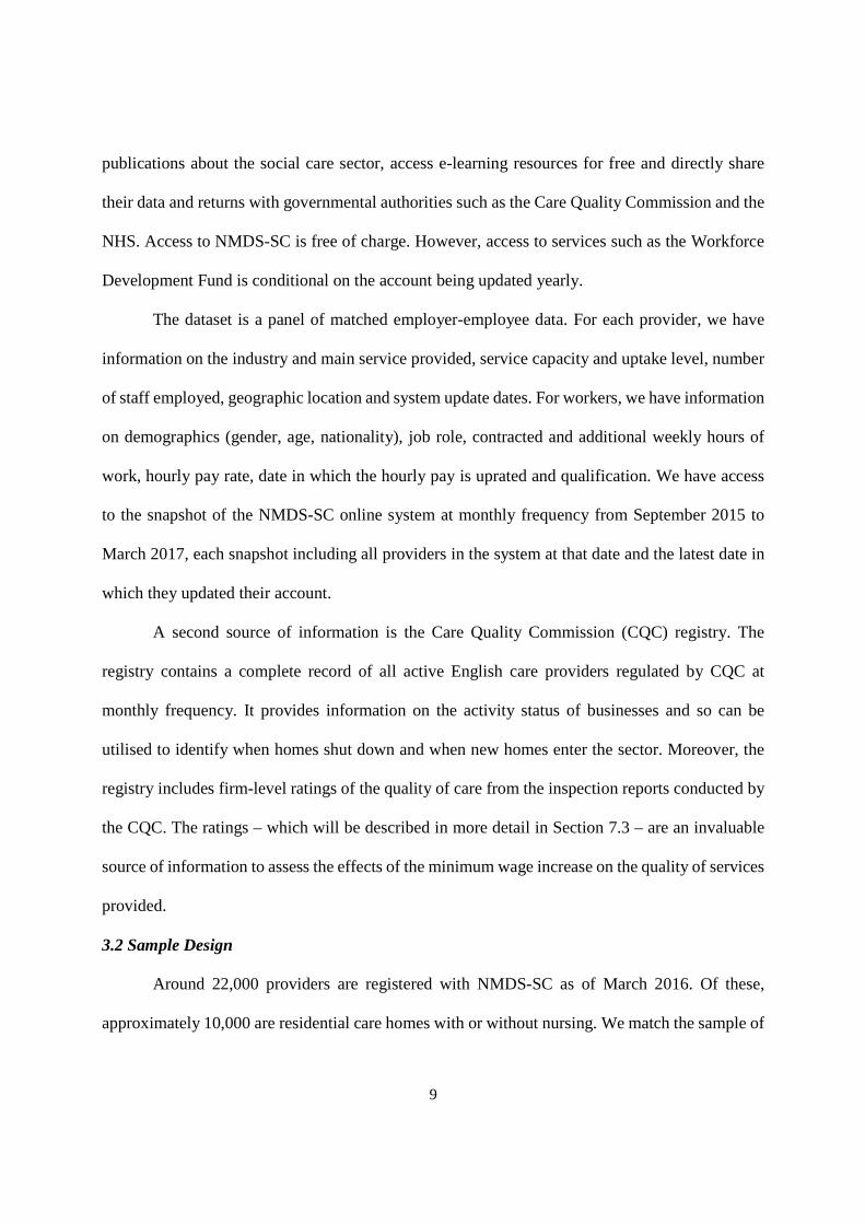
publications about the social care sector, access e-learning resources for free and directly share

their data and returns with governmental authorities such as the Care Quality Commission and the

NHS. Access to NMDS-SC is free of charge. However, access to services such as the Workforce

Development Fund is conditional on the account being updated yearly.

The dataset is a panel of matched employer-employee data. For each provider, we have

information on the industry and main service provided, service capacity and uptake level, number

of staff employed, geographic location and system update dates. For workers, we have information

on demographics (gender, age, nationality), job role, contracted and additional weekly hours of

work, hourly pay rate, date in which the hourly pay is uprated and qualification. We have access

to the snapshot of the NMDS-SC online system at monthly frequency from September 2015 to

March 2017, each snapshot including all providers in the system at that date and the latest date in

which they updated their account.

A second source of information is the Care Quality Commission (CQC) registry. The

registry contains a complete record of all active English care providers regulated by CQC at

monthly frequency. It provides information on the activity status of businesses and so can be

utilised to identify when homes shut down and when new homes enter the sector. Moreover, the

registry includes firm-level ratings of the quality of care from the inspection reports conducted by

the CQC. The ratings – which will be described in more detail in Section 7.3 – are an invaluable

source of information to assess the effects of the minimum wage increase on the quality of services

provided.

3.2 Sample Design

Around 22,000 providers are registered with NMDS-SC as of March 2016. Of these,

approximately 10,000 are residential care homes with or without nursing. We match the sample of

10

residential care homes with the CQC registry of active locations from September 2015 to March

2017, from which we can obtain information on whether a firm is active or closed in a given month.

Our sample comprises care homes that meet the following three requirements: (i) being open in

March 2016, (ii) having a record on NMDS-SC for all the months in which the firm is open

according to the CQC registry and (iii) having updated their NMDS-SC account at least once after

March 2016. This selection leaves us with a balanced panel of 4,134 firms that are active in March

2016 and remain open until March 2017.

3.3 Descriptive Statistics

Table 1 reports descriptive statistics for the balanced sample of firms from one month

before the NLW introduction that took place in April 2016 to three, six and twelve months after.

The relatively low hourly pay and large fraction of workers aged 25 and over in the pre-NLW data

confirm the high vulnerability of the care home sector to the NLW introduction, which therefore

appears particularly pertinent to study the impact of the NLW as it potentially affected a large

proportion of workers. A second feature of the data is that average wages rise in the months after

the NLW introduction, by 2, 3 and 4 percent after one, two and four quarters respectively. This is

true both in the full sample of workers and for those aged under 25 and 25 and over. The

progressive rise in average wages over time is due to the fact that firms update their records on

NMDS-SC over time – an aspect we will discuss more in depth in the next section.

The statistics reported in Table 1 also show that the care home sector is characterised by

small-to-medium size establishments working close to full capacity (the occupancy rate measured

as the ratio of residents to beds is above 90 percent). Mean and median employment are

approximately 39 and 32 respectively. The workforce is predominantly female (84 percent), on

average older than 40 and working approximately 30 hours per week. The main occupation in this

11

sector is care assistant, which accounts for 56 percent of the workforce. Only 4 percent of the

workers hold a nursing qualification. All these characteristics remain fairly constant before and

after April 2017, suggesting that the NLW did not induce a compositional change in the productive

structure of care homes.

3.4 Representativeness

It is important to assess the representativeness of our sample as compared to the full

population of care homes and their workforce. Estimates from Skills for Care indicate that the

NMDS-SC data cover more than 50 percent of the workforce in CQC regulated homes, suggesting

that the system might provide a good representation of the sector in England. We also compare the

characteristics of our sample with statistics on firms and workers in the care home sector that we

derive from the ONS Business Registry and the Labour Force Survey. According to the 2016 ONS

Business Registry, firms in the residential care industry for the elderly and disabled have an

average firm size that matches the one in our sample (approximately 37 on ONS). Similarly,

looking at baseline characteristics for carers in the LFS for the first quarter of 2016, we find that

they line up quite satisfactorily with those in our sample of workers, as in the LFS the proportion

of female carers is 0.85, average age 42, average hourly wage £7.77 and average weekly hours

worked 34. Overall, these statistics are reassuring of our ability to draw any general conclusions

from the analysis of the data we undertake.

4. Wages and Employment Impacts of National Living Wage Introduction

4.1 Wages Impact

As previously noted, the residential care home sector appears to be potentially vulnerable to the

NLW introduction given its wage structure and workforce’s age composition. In this section we

confirm that the NLW had real “bite” in the care home sector and generated the expected effects

12

on hourly wages and their distribution. This is clearly a necessary condition before analysing the

employment and other economic consequences of minimum wages.

Table 2 reports results on the first part of the investigation of the impact of the NLW

introduction on wages. It shows several measures of the bite of the NLW. Specifically, these are

the proportion of workers paid less than the NLW (or less than the age-specific NMW if younger

than 25), the percentage paid exactly at the minimum and the wage gap. The latter is a measure of

how much wages would have to increase in a given firm in order to meet the new legal

requirements and is computed as follows:

���� = ∑ ℎ�� max {������ − ���, 0}�∑ ℎ�� ����

(1)

where ℎ�� is weekly hours worked by worker � in firm �, ��� is the hourly wage of worker � in firm

� and ������ is the new age-specific minimum wage (i.e. £3.87 for workers aged 16-17, £5.30 for

workers aged 18-20, £6.70 for workers aged 21-24 and £7.20 for older workers). As before, pre-

and post-NLW statistics are reported for care homes in the balanced panel.

The residential care sector has clear potential to be heavily affected by the NLW. Around

55 percent of workers aged 25 and over, who would be legally affected by the NLW, were paid

below the NLW before it was introduced and only 3 percent were paid exactly at £7.20. Given the

small proportion of young workers, similar figures are found for the whole sample of workers (51

and 3 percent respectively). The NLW wage gap averaged 4 percent before the NLW introduction,

confirming the high vulnerability of the sector to the minimum wage increase.

Results in Table 2 also demonstrate that the NLW strongly affected care home wages. The

post-NLW data show a larger drop in underpayment over time (of 16, 18 and 29 percentage points

after three, six and twelve months respectively), a halving of the wage gap and a noticeable spike

of up to 20 percent at the new minimum. A substantial distributional impact of the NLW on wages

13

can also be seen by looking at Figure 1, which plots the hourly wage distribution for care assistants

one month before and three, six and twelve months after the NLW introduction. The charts provide

compelling evidence of the sizable compression effect the NLW had at the bottom of the hourly

wage distribution and the emergence of a sharp spike at the new minimum after its introduction.

Among care assistants, the spike reached 20 percent in June 2016, 26 percent in September 2016

and 30 percent by March 2017.

One issue is that not all care homes update their records at the same time, nor with the same

frequency. In order to avoid sample selection driven by unobservable worker and firm

characteristics that may be correlated with the timing and frequency of updating, we do not

condition our sample on a specific update date and only require that a firm update its records once

in the twelve months after April 1st 2016.10 As a result, some of the post-NLW data are not updated.

For this reason, the spike at £7.20 as well as the statistics presented in Table 2 change progressively

over time. Nonetheless, the spike in June 2016 is already remarkably sizable.

To confirm the role of updates in shaping the progressive change of the wage distribution,

Figure 2 replicates Figure 1 for a subsample of workers whose wages were updated within given

time windows. Specifically, the top left panel includes workers with wage updates between

October 2015 and March 2016, the top right panel between April and June 2016, the bottom left

panel between April and September 2016, and the bottom right panel between April 2016 and

March 2017. The histograms show a spectacular spike at £6.70 in the pre-NLW period, and an

even larger, sharper spike of around 40 percent at the new minimum in the post-NLW period.

10 Approximately 90 percent of NMDS-SC users update within a year.

14

Having established a strong impact of the minimum wage on wages in the care home

industry, we now show that homes with the highest potential to be affected were indeed the most

affected. To this end, we estimate hourly wage change equations of the following form:

����,� = �� + ��� !�,�"� + #�,�"�$ %� + &�,� (2)

where ����,� is the change in the natural logarithm of the average wage in firm � between March

2016 and three, six or twelve months after; � !�,�"� is a measure of the NLW bite at the care

home level, that is either the initial proportion of workers paid below the NLW or the NLW wage

gap; # is a vector of pre-NLW firm-level characteristics including the proportion of female

workers, average age, the proportion working as care assistants, the proportion with nursing

qualification, the occupancy rate and a set of indicators for the nine English regions.

The parameter of interest is ��, which measures the relationship between wage growth and

the minimum wage. The parameter is identified from between-home variation in pre-NLW wage

levels and it therefore identifies the causal effect of the minimum wage on wage growth only if –

absent the minimum wage change – there was no relationship between the initial level of wages

and wage growth. We provide supporting evidence for this identifying assumption by looking at

the relationship between wage growth and initial wages around a time in which no minimum wage

change took place. To this end, we select a balanced sample of firms active between March 2015

and March 2016 from NMDS-SC adopting the exact same criteria we use for our main sample.

We consider whether there is any relationship between wage growth and the logarithm of initial

wages between March 2015 and three and six months after, a period over which the NMW

remained unaltered.11 Results are reported in panel A of Table A1 in Appendix A2. The

11 As of March 2015, the NMW rates were as follows: an adult minimum rate for workers aged 21 and over of £6.50, a youth development rate of £5.13 for those aged 18-20, a youth minimum of £3.79 for 16-17 year olds and an

15

coefficients in columns (1) and (4) indicate a significant and negative relationship between wage

growth and initial wage levels in 2015. However, as compared to the period surrounding the NLW

introduction (reported in columns (2) and (5)), the magnitude of these effects is much smaller in

absolute value. As a result, the difference between the two coefficients remains strongly negative

and significant (see columns (3) and (6)), indicating that there was a clear shift in the relationship

between wage growth and initial wages between the two periods.

Table 3 reports the estimated wage equations for the balanced panel of firms. Panel A refers

to ����,� between March 2016 and June 2016, panel B between March 2016 and September 2016,

and panel C between March 2016 and March 2017. For each of the three panels, the specifications

in columns (1) and (2) report the estimated coefficient �� for a model in which � !�,�"� is the pre-

NLW proportion of workers paid below the NLW (or their age-specific NMW if less than 25 years

old), while columns (3) and (4) for a model using the wage gap as main regressor. The regression

models in columns (2) and (4) include the above-listed firm-level controls.

In all cases there is significant evidence of larger increases in wages in homes with more

low-wage workers in the pre-NLW period, as measured by the low-wage proportion or the wage

gap. According to the regression estimates in panel C, a one standard deviation increase in the

proportion of low-paid workers (corresponding to a 33 percentage point change) implies a 1.6

percentage-point faster wage growth on a baseline of 4 percent. A similar effect of 1.6 percentage

point faster wage growth is found as a result of a one standard deviation increase in the wage gap

(corresponding to a 4 percentage point change). Both effects are sizable and establish a strong and

apprentice rate of £2.73. Since the NMW was then uprated in October 2015, in Table A1 we only consider changes between March and June, and March and September 2015.

16

significant relationship between minimum wages and wage growth. We find comparable results

when looking at weekly earnings growth as shown in Table A2 in Appendix A2.12

4.2 Employment Impact

Having established that the NLW had important wage and wage structure effects, we next

consider a “second stage” of whether or not the wage cost shock induced by the NLW had

consequences on employment and total hours. We start by estimating reduced-form employment

and total hours change equations similar to the wage equations illustrated in the previous

subsection. Specifically, we regress the change in the logarithm of the number of employees and

of total weekly hours (��'�,�) on measures of the NLW bite, as follows:

��'�,� = �) + �)� !�,�"� + #�,�"�$ %) + *�,� (3)

where � ! and # are defined as before.

Similarly to the wage equation, the identifying assumption for �) is that – absent the

minimum wage increase – there would be no relationship between initial wages and employment

(or total hours) growth. We investigate whether the relationship between employment growth and

initial wages changed in the period surrounding the NLW introduction as compared to a year

before – a period with no minimum wage changes. Panels B and C of Table A1 in Appendix A2

report the results of this exercise for employment and total hours growth respectively.

The first thing to notice is that the correlations between employment (total hours) growth

and initial wages are much weaker than those found for wage growth. Interestingly, the estimated

coefficients for the “no policy” period are all very small in size and statistically insignificant, which

we take as evidence that the model’s identifying assumption seems to be supported by the data.

12 The coefficients reported in Columns (1) to (4) in the three panels of Table A2 in Appendix A2 closely match those obtained for hourly wages, suggesting that the wage elasticity of weekly earnings is approximately one. This is indeed what we find in columns (5) and (6) where we estimate the structural form as described in section 4.2.

17

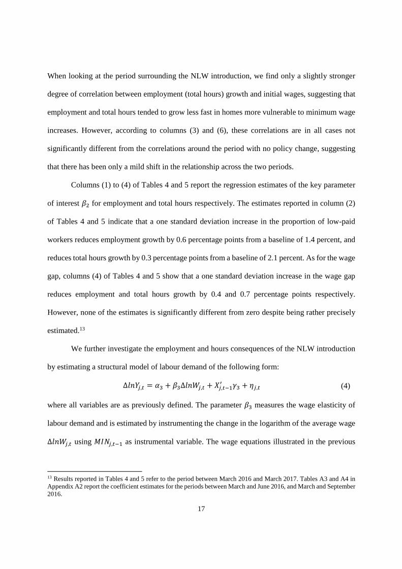
When looking at the period surrounding the NLW introduction, we find only a slightly stronger

degree of correlation between employment (total hours) growth and initial wages, suggesting that

employment and total hours tended to grow less fast in homes more vulnerable to minimum wage

increases. However, according to columns (3) and (6), these correlations are in all cases not

significantly different from the correlations around the period with no policy change, suggesting

that there has been only a mild shift in the relationship across the two periods.

Columns (1) to (4) of Tables 4 and 5 report the regression estimates of the key parameter

of interest �) for employment and total hours respectively. The estimates reported in column (2)

of Tables 4 and 5 indicate that a one standard deviation increase in the proportion of low-paid

workers reduces employment growth by 0.6 percentage points from a baseline of 1.4 percent, and

reduces total hours growth by 0.3 percentage points from a baseline of 2.1 percent. As for the wage

gap, columns (4) of Tables 4 and 5 show that a one standard deviation increase in the wage gap

reduces employment and total hours growth by 0.4 and 0.7 percentage points respectively.

However, none of the estimates is significantly different from zero despite being rather precisely

estimated.13

We further investigate the employment and hours consequences of the NLW introduction

by estimating a structural model of labour demand of the following form:

��'�,� = �+ + �+����,� + #�,�"�$ %+ + ,�,� (4)

where all variables are as previously defined. The parameter �+ measures the wage elasticity of

labour demand and is estimated by instrumenting the change in the logarithm of the average wage

����,� using � !�,�"� as instrumental variable. The wage equations illustrated in the previous

13 Results reported in Tables 4 and 5 refer to the period between March 2016 and March 2017. Tables A3 and A4 in Appendix A2 report the coefficient estimates for the periods between March and June 2016, and March and September 2016.

18

section can be therefore considered as the first stage of this instrumental variable model and show

that the instrument is relevant. To be valid, an instrument should also satisfy the exclusion

restriction and be as good as randomly assigned, i.e. our measures of the NLW bite should only

affect the outcome through their impact on wage growth and be uncorrelated with any other

proximate determinant of employment or total hours growth. Although neither of these two

assumptions can be formally tested, the evidence in Table A1 (panels B and C) seems to support

the assumption of random assignment.

Estimates of the structural elasticities are reported in columns (5) and (6) of Tables 4 and

5, using the initial proportion of low paid and the wage gap as instruments for the wage change

respectively.14 The estimated wage elasticity of employment ranges between -0.23 and -0.41

(Table 4), while that of hours is between -0.21 and -0.44 (Table 5). Evaluated at an average wage

growth of approximately 4 percent, these elasticities indicate that headcount employment would

drop by 0.9-1.6 percent and total hours by 0.8-1.8 percent. The estimated employment and total

hour elasticities are modest, bit relatively large compared to many of the estimates in the recent

minimum wage literature. However, none of the structural elasticities nor the reduced-form

estimates is significantly different from zero, leading to the conclusion that there is no clear

evidence of detrimental employment, nor hours effects, of the NLW introduction.15, 16

14 In Tables 4 and 5, both the dependent variable and the main regressor are computed as the change between March 2016 and March 2017. Tables A3 and A4 in Appendix A2 report estimates for the period between March and June 2016 in panel A, and between March 2016 and September 2016 in panel B. 15 In order to check that our results are not driven by the lack of updating by firms, we estimate the wage, employment and total hour equations on the subsample of firms that updated the wages of at least 50 percent of their workers in the period between October 2015 and March 2016, and in the period after March 2016. All results hold in this subsample and are available upon request. 16 The absence of employment effects could in fact mask changes in the composition of the workforce, for a given level of employment. We find no evidence of differential levels of inflows, outflows and total flows as a consequence of the NLW introduction, which leads us to exclude the presence of such compositional changes.

19

5. Wage and Employment Spillovers

5.1 Wage Spillovers Down the Wage Distribution

The NLW increased the minimum wage for workers aged 25 and over to £7.20 per hour, but left

the minimum wage rate for workers aged 21-24 at the October 2015 level of £6.70 per hour. It is

an interesting question, then, whether care homes left wages for workers under 25 unchanged at

the old NMW, or whether they decided to also raise them, perhaps for reasons of administrative

simplicity or inequality aversion within the firm.

In this subsection, we provide compelling graphical evidence that it is indeed the case that

the NLW generated positive spillover effects on the wages of younger cohorts. Figure 3 shows the

evolution of the hourly wage distribution for care assistants aged under 25 from one month before

to twelve months after the NLW introduction. Figure 4 reproduces the same graphs on the

subsample of workers whose hourly wages were updated between October 2015 and March 2016

(top left panel), between April 2016 and June 2016 (top right panel), between April 2016 and

September 2016 (bottom left panel), and between April 2016 and March 2017 (bottom right panel).

Strikingly, we observe a spectacular spike located at the new adult minimum after April 2016, and

a strong wage compression in the bottom half of the distribution. Both the location and size of the

spike, and the amount of bottom wage compression are analogous to what we found for the entire

sample of care assistants over all age groups. According to Figure 4, while 34 percent of care

assistants aged under 25 were paid at the NMW in March 2016; up to 35 percent of younger

workers are at the new NLW after its introduction.

We complement the graphical analysis illustrated above by performing some regression

analysis of spillover effects on wages. Firstly, we run a simple reduced-form model of the growth

20

rate of hourly wages for workers under 25 as a function of measures of the NLW bite for older

workers. The reduced-form model reads as follows:

����,�- = �. + �.� !�,�"�/ + #�,�"�$ %. + 0�,� (5)

where ����,�- is the change in the natural logarithm of the average wage of workers under 25 in

firm � between March 2016 and three, six or twelve months after; � !�,�"�/ indicates alternatively

the initial proportion of workers aged 25 and over that are paid below the NLW, or the NLW wage

gap for older workers; # is the vector of pre-NLW firm-level characteristics that we described in

our previous analyses. The reduced-form estimates are reported in columns (1) to (4) of Table 6.

We also perform a structural estimation of the cross wage elasticity between wages of

younger workers and adult workers. In the structural estimation, we regress the change in log

average wages for younger workers ����,�- on the change in log average wages for older workers

����,�/ , and we instrument the latter using � !�,�"�/ as instrumental variable. The structural model

reads as follows:

����,�- = �1 + �1����,�/ + #�,�"�$ %1 + 2�,� (6)

Estimates of the structural cross elasticity parameter �1 are reported in columns (5) and (6)

of Table 6, where we respectively use the proportion of low paid workers among those aged 25

and over, and the wage gap for older workers as instruments. The first stage regression coefficients

are reported in Table A5 in Appendix A2.

All the estimates in Table 6 indicate significantly positive spillovers on the hourly wages

of younger workers and cross elasticities of approximately 0.7. According to columns (2) and (4)

of panel C, a one standard deviation increase in the proportion of older workers paid below the

NLW or in the adult wage gap (corresponding respectively to 34 and 4 percentage points in the

estimation sample) are associated with a 1.3 and 1.2 percentage point faster wage growth for

21

younger workers, on a baseline youth wage growth of 4.1 percent. Cross-elasticity estimates

indicate that a one percent increase in average adult wages induces a 0.7 percent increase in

average youth wages.17,18

5.2 Employment and Total Hours Spillovers

Having documented significant and positive spillovers on wages that resulted from the

changed minimum wage structure, we also test for the presence of spillover effects on employment

and total hours for workers under 25. Indeed, firms might be induced to raise wages of younger

workers for reasons of fairness or simplicity, but at the same time may reduce youth employment

along the intensive or extensive margin if youth productivity is lower than the uprated wage. We

adopt a methodology similar to the one used to investigate wage spillovers, regressing the change

in the share of total employment aged under 25 and the change in the share of total hours worked

by workers under 25 on (i) measures of the NLW bite amongst workers aged 25 and over

(� !�,�"�/ ) and (ii) ����,�/ instrumented using � !�,�"�/ . Reduced-form estimates of employment

and total hours spillovers are reported in columns (1) to (4) of Tables 7 and 8, while structural

cross wage elasticities of demand are reported in columns (5) and (6).19 Overall we find no

statistically significant evidence of negative spillovers at the extensive and the intensive margins

of employment, suggesting that the residential care home sector has so far coped with the NLW

17 We also investigated whether the size of wage spillovers changes with the bite of the NLW on older workers. There was no evidence of statistically significant differential effects between firms with a proportion of low-paid older workers above and below the mean in the sample (and similarly for firms with an NLW gap for older workers above and below the mean in the sample). 18 We also consider spillover effects on weekly earnings. As reported in Table A6 in Appendix A2, the coefficients are not as precisely estimated as those of the wage spillover equations, except for those in panel C that are highly statistically significant. Nonetheless, in none of the estimates in columns (5) and (6) we can reject a coefficient magnitude comparable to the corresponding effect in Table 6.19 Tables 7 and 8 report estimates for the period between March 2016 and March 2017. Estimates for the periods between March and June 2016, and March and September 2016 can be found in Tables A7 and A8 in Appendix A2.

22

introduction since it managed to raise wages of legally unaffected workers without reducing

employment.20

6. Reasons for Wage Spillovers

6.1 Wage Spillovers in the Domiciliary Care Sector

In this and the next subsection, we investigate potential explanations of why the wage spillovers

that we uncovered in the previous analysis may have come about. A first obvious candidate for

explaining why we observe positive spillovers on younger workers is that either workers or firms

are concerned with the fairness of the within-home wage structure and prefer that workers doing

the same job receive the same wage, even though some of them may be more productive. There is

considerable evidence for such preferences for fairness in the minimum wage literature. Survey

data on fast food restaurants in Texas and administrative data on the retail sector in Finland indicate

that employers have been reluctant to apply youth sub-minima (Katz and Krueger, 1991; 1992;

Böckerman and Uusitalo, 2009), and laboratory experiments have shown that minimum wage

increases generate entitlement effects and change workers’ perceptions of what a fair wage is (Falk

et al., 2006).

It seems plausible that if workers’ preferences for “equal pay for equal job” were entirely

responsible for the emergence of wage spillover effects, the latter should be stronger for employees

working in team or with direct sight of their colleagues while working. In order to test whether

spillover effects are driven by workers’ as opposed to employers’ equity concerns, we replicate

20 The lack of spillovers on employment could in fact mask a change in the composition of the younger workforce, for a given proportion of employees aged under 25. An analysis of inflows, outflows and total flows of younger workers indicated that – if anything – firms that had the larger wage spillovers experienced lower levels of churning amongst the younger segments of their workforce, thus excluding significant compositional changes in response to the wage cost shock.

23

our analysis of spillover effects in the domiciliary care sector for which we have data on NMDS-

SC.

Domiciliary care is a social care service provided to people who live in their own houses

and require assistance with personal care routines, household tasks such as cleaning and cooking,

or any other activities they may need to live independently. Domiciliary care assistants typically

work individually, drive their own car to visit customers’ homes, and are often contracted on

flexible working hours or zero-hour contracts since domiciliary care work tends to be organised

into short and fragmented home visits. Given the nature and organisation of work, workers

employed by domiciliary care agencies tend to have limited face-to-face interactions with co-

workers on the job and are unlikely to be fully aware of their working conditions. If downward

wage spillovers were entirely due to workers’ fairness preferences, we would expect them to be

milder in the domiciliary care sector than the care homes one, ceteris paribus.

The summary statistics reported in Table 9 illustrate the main differences between firms

and workers in the care home and domiciliary care sectors.21 While the gender and age composition

is essentially identical across the two sectors, and wage differentials are relatively limited, working

arrangements diverge strikingly. The incidence of zero-hour contracts is nine times as large in the

domiciliary care sector when considering workers of all ages and five times as large for workers

aged under 25. Similarly the proportion of workers on alternative work arrangements, i.e.

employed with temporary, bank or agency contracts, is almost twice as large in the domiciliary

care sector (14 against 8 percent). These substantial differences corroborate the notion that

domiciliary care work schedules are inherently fragmented as the nature of the job would suggest.

21 The sample of care homes is the one used in the previous analysis, while the sample of domiciliary care agencies is selected following the same criteria used to select the sample of care homes and illustrated in section 3.2.

24

We replicate the analysis of wage spillover effects on the sample of domiciliary carers.

Figure 5 shows the evolution of the hourly wage distribution for domiciliary carers aged under 25

from one month before to twelve months after the NLW introduction. It is based on the subsamples

of workers whose hourly wages were updated between October 2015 and March 2016 (top left

panel), between April 2016 and June 2016 (top right panel), between April 2016 and September

2016 (bottom left panel), and between April 2016 and March 2017 (bottom right panel).22 The

similarity with the patters observed for care assistants in the care home sector is striking. A large

spike at the new minimum and a strong wage compression in the bottom half of the wage

distribution clearly emerge after April 2016. The size of the spike is in line with the one found for

care assistants aged under 25, with approximately 31 percent of young domiciliary carers being

paid exactly £7.20. We also estimate the empirical models (5) and (6) on the domiciliary care

sample. Results are reported in Table 10. None of the structural cross elasticities reported in

columns (5) and (6) of panels A, B and C is statistically different from one, indicating that wages

for younger workers increased one for one with wages of adult workers.23,24

Therefore, in spite of the remarkably different working arrangements documented above,

domiciliary care workers experience wage spillovers very similar in magnitude to those we

identified in the care home industry. We interpret this evidence as supportive of the fact that team

22 Figure A2 in Appendix A2 reproduces the same graph on the full sample of domiciliary carers aged under 25. 23 Table A9 in Appendix A2 reports the coefficient estimates of the wage equations in the sample of domiciliary care agencies. Results in columns (1) and (2) of panels A, B and C are very much in line with those reported in Table 3 for the sample of care homes. Results in columns (3) and (4) are instead smaller in magnitude and less precisely estimated. Given the high incidence of zero-hour contracts in the domiciliary care sector, the NLW gap appears less appropriate as a measure of the NLW bite in this context as opposed to the care home one (Datta et al., forthcoming). 24 The first-stage coefficients for the wage spillover equations in the domiciliary care sector are reported in Table A10 in Appendix A2.

25

dynamics and worker-specific preferences for fairness are not key drivers of downward minimum

wage spillovers.25

6.2 Evidence on the “fairness” hypothesis

The evidence presented in the previous subsection seems to exclude a strong role for

workers’ preferences alone in within-firm wage setting. Two additional theories could explain the

emergence of downward wage spillovers. The first is fairness concerns and inequality aversion by

employers. The second is administrative simplicity, whereby employers try to minimise the costs

of managing a diverse wage structure and of individual-level bargaining. While we cannot

formally test which of these two alternative theories has the largest bearing, in this section we

discuss evidence we gathered from a survey of care homes that seems to support the “fairness

hypothesis”.

For an earlier project funded by the Low Pay Commission, we ran a survey of English care

homes. We obtained information on all care homes in England from the CQC directory and sent

questionnaires to all homes in January and February 2016 for the pre-NLW part of the survey, and

in late June, August and November 2016 for the post-NLW part of the survey. We obtained a total

of 1390 responses in the pre-NLW survey and of 827 responses in the post-NLW survey that were

provided by the owner manager of the care homes.26 In both the pre- and post-NLW surveys, we

asked respondents about their views on the level of the NLW. Before the NLW introduction, 42.7

percent of respondents believed that the level of the NLW was about right, while 15.0 percent

thought it too low and 37.6 percent too high. Interestingly, after the implementation of the new

wage floor, respondents appear to be much more favourable to the minimum wage floor, with 52.5

25 For the sake of completeness, we also investigate employment and total hours spillovers in the domiciliary care sector in Tables A11 and A12 in Appendix A2. None of the estimated coefficients is statistically significantly different from zero. 26 More information on the survey of care homes is available upon request.

26

percent considering it about right, 19.7 percent too low and only 23.7 percent too high.27 In the

post-NLW survey we asked respondents to leave a verbal comment about what they believed

would be the impact of the NLW on their business. While it is not uncommon for respondents to

state that it is fair for a worker to earn a “living wage”, none of the replies refers to administrative

simplicity and bargaining costs.

We perform a back-of-the-envelope calculation and estimate what the average

counterfactual savings from paying all care assistants their age-specific minima would be. It turns

out that, if all care assistants were paid their minimum wage, the total wage bill would decrease

by 2.6-2.9 percent.28 The same figure would drop to 1.2-1.3 percent if only care assistant under 25

were paid their age-specific minima. For a labour share of total costs of approximately 60 percent

and assuming no scope for efficiency wages, we conclude that after the NLW introduction

employers have been willing to take a profit hit of up to 1.7 percent – above and beyond the 2.4

percent needed to meet the NLW requirements – when raising wages above the legal minimum.29

7. Other Margins of Adjustment

Given the lack of evidence of employment effects in spite of significant wage increases for both

legally affected and unaffected workers, this section explores whether the minimum wage increase

had an impact on outcomes other than employment and total hours. It is possible that firms respond

to the wage cost shock by adjusting other margins, such as prices, profits, productivity and the

quality of care services. We consider these outcomes in the following subsections.

27 See Table A13 in Appendix A2 for results on the balanced panel. 28 The age specific minima are the NLW of £7.20 for those aged 25 and over, the NMW for those under 25, a youth development rate of £5.30 for those aged 18-20, a youth minimum of £3.87 for 16-17 year olds and an apprentice rate of £3.30. 29 We obtain an estimate of the labour share of total costs from our post-NLW survey, where we ask the question “Approximately what percentage of your total costs are labour costs?”.

27

7.1 Price setting and resident intake

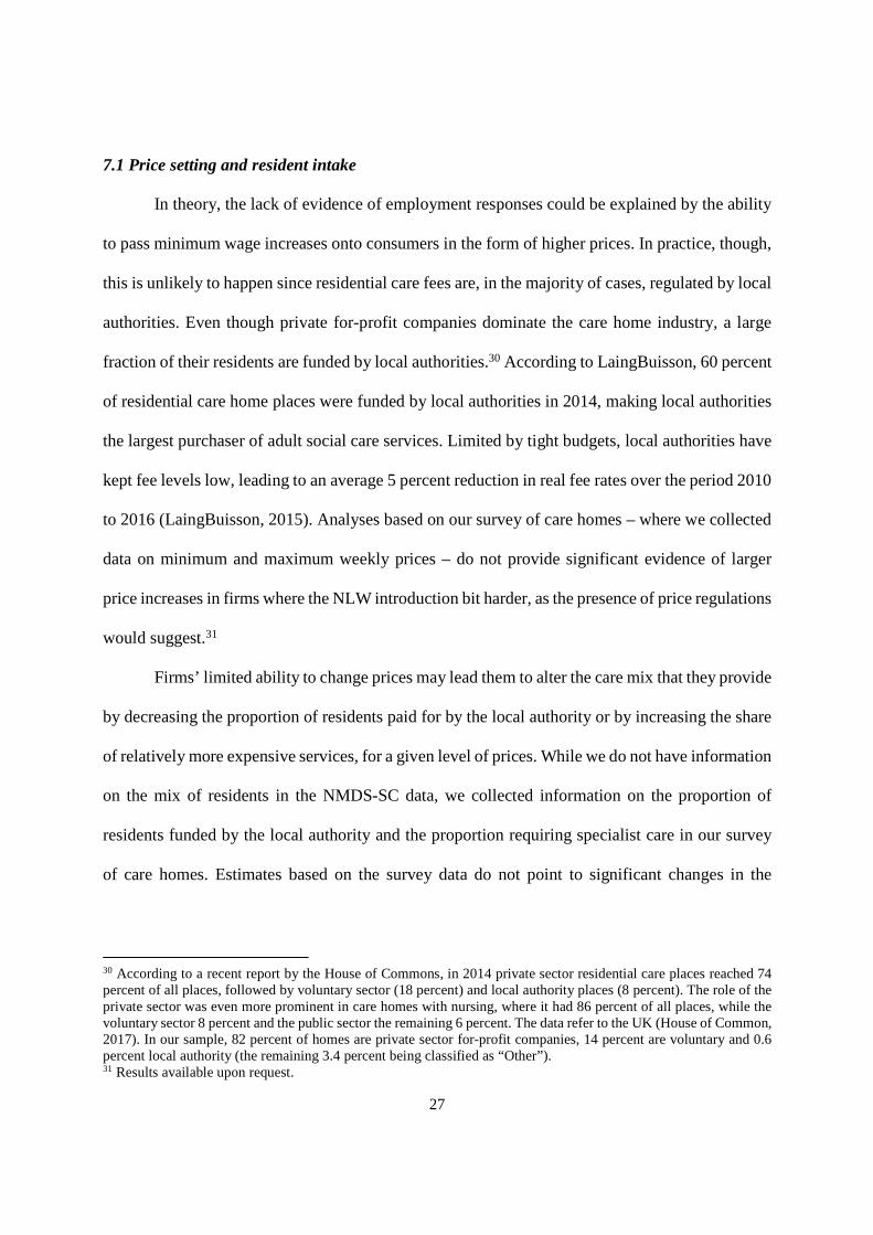
In theory, the lack of evidence of employment responses could be explained by the ability

to pass minimum wage increases onto consumers in the form of higher prices. In practice, though,

this is unlikely to happen since residential care fees are, in the majority of cases, regulated by local

authorities. Even though private for-profit companies dominate the care home industry, a large

fraction of their residents are funded by local authorities.30 According to LaingBuisson, 60 percent

of residential care home places were funded by local authorities in 2014, making local authorities

the largest purchaser of adult social care services. Limited by tight budgets, local authorities have

kept fee levels low, leading to an average 5 percent reduction in real fee rates over the period 2010

to 2016 (LaingBuisson, 2015). Analyses based on our survey of care homes – where we collected

data on minimum and maximum weekly prices – do not provide significant evidence of larger

price increases in firms where the NLW introduction bit harder, as the presence of price regulations

would suggest.31

Firms’ limited ability to change prices may lead them to alter the care mix that they provide

by decreasing the proportion of residents paid for by the local authority or by increasing the share

of relatively more expensive services, for a given level of prices. While we do not have information

on the mix of residents in the NMDS-SC data, we collected information on the proportion of

residents funded by the local authority and the proportion requiring specialist care in our survey

of care homes. Estimates based on the survey data do not point to significant changes in the

30 According to a recent report by the House of Commons, in 2014 private sector residential care places reached 74 percent of all places, followed by voluntary sector (18 percent) and local authority places (8 percent). The role of the private sector was even more prominent in care homes with nursing, where it had 86 percent of all places, while the voluntary sector 8 percent and the public sector the remaining 6 percent. The data refer to the UK (House of Common, 2017). In our sample, 82 percent of homes are private sector for-profit companies, 14 percent are voluntary and 0.6 percent local authority (the remaining 3.4 percent being classified as “Other”). 31 Results available upon request.

28

proportion of local authority funded residents, but are suggestive, albeit at the margins of statistical

significance, of an increase in the proportion of residents requiring specialist care.32

7.2 Productivity

A margin that firms may try to improve in response to the increase in costs is productivity.

In order to explore this hypothesis, we construct a measure of productivity as the logarithm of

residents per worker hour. We regress the change in productivity against measures of the NLW

bite and the change in the logarithm of average wages appropriately instrumented. According to

the estimates reported in Table 11, there is no evidence of larger productivity improvements by

those firms that were more heavily affected by the NLW introduction.33

7.3 Quality of care services

Another possibility is that firms respond to the cost shock by reducing the quality of care

services provided. We have information on the quality of care from the inspection reports

conducted by the CQC. The CQC is the independent regulator of health and adult social care in

England. It is responsible for setting standards of care and for monitoring, inspecting and rating

adult social care providers, to make sure that they meet fundamental standards of quality and

safety. At the heart of CQC’s regulatory activity, the rating process is based on periodic inspections

of care providers followed by the publication of reports showing the evaluation of the quality of

care. The ratings are articulated into five key lines of enquiry and an overall judgement. The five

lines of enquiry ask if the service is safe, effective, caring, responsive to people’s needs and well-

32 Results available upon request. 33 Results in Table 11 refer to the period between March 2016 and March 2017. Analogous results for the periods between March and June, and March and September 2016 are reported in Table A14 in Appendix A2.

29

led, while the overall judgement is an aggregation of these five dimensions.34 The rating can be

“outstanding”, “good”, “requires improvement” or “inadequate”.35

We have access to the most recent firm-level CQC ratings as of March 2016 and March

2017, and can link them to observations in the NMDS-SC database. Of the 2480 homes that we

could match, 931 had been inspected and rated before and after the NLW introduction. Figure A3

in Appendix A2 displays the distribution of ratings by key line of enquiry as of March 2016 for

the full sample (Panel A) and for the subsample of firms with rating both before and after March

2016 (Panel B). In a similar fashion, Panels A and B of Figure A4 in Appendix A2 show the

distribution of the change in ratings between March 2016 and March 2017 for the two samples.

Ratings tend to be concentrated in the mid-range categories, with approximately 65 percent of

homes providing a good overall service and 35 percent requiring improvement as of March 2016

(Panel A of Figure A3). The subgroup of firm that were inspected both before and after March

2016 tend to have poorer performances across all lines of enquiry (Panel B of Figure A3),

suggesting that performance and the frequency of inspections might be negatively correlated.

Ratings vary upward or downward between March 2016 and March 2017 for approximately 50

percent of the sample inspected in both periods (Panel B of Figure A4).

We investigate whether the NLW introduction caused a change in the quality of care

services by running regression models similar to equations (3) and (4), where – for each line of

34 The key lines of enquiry are specified as follows. Safe: residents are protected from abuse and avoidable harm. Effective: care, treatment and support achieves good outcomes, helps residents maintain quality of life and is based on the best available evidence. Caring: staff involve and treat residents with compassion, kindness, dignity and respect. Responsive: services are organised so that they meet the resident’s needs. Well-led: the leadership, management and governance of the organisation make sure it is providing high-quality care that is based around the resident’s individual needs, it encourages learning and innovation, and it promotes an open and fair culture. Further details can be found at http://www.cqc.org.uk/what-we-do/how-we-do-our-job/five-key-questions-we-ask. 35 Outstanding: the service is performing exceptionally well. Good: the service is performing well and meeting CQC’s expectations. Requires improvement: the service is not performing as well as it should and has been told that it must improve. Inadequate: the service is performing badly and CQC has taken action against the person or organisation that runs it. Further details can be found at www.cqc.org.uk/what-we-do/how-we-do-our-job/ratings.

30

enquiry – we regress the change in rating between March 2016 and March 2017 against measures

of the NLW bite (� !�,�"�) and against the change in the logarithm of the average wage (����,�)

instrumented with � !�,�"�. As pointed out before, care homes with lower initial ratings are more

likely to be inspected in the post-NLW period, i.e. are more likely to experience a change in ratings.

If initial ratings are correlated with the initial level of wages and, in turn, with the bite of the NLW,

our estimates of the causal effect of the NLW on the quality of care would be biased. To account

for the potential confounding effect of initial ratings, we include them among the controls.

Results are reported in Table 12, where Panel A refers to the overall rating and subsequent

panels refer each to one of the five key lines of enquiry. Both reduced-form and structural-form

coefficients are negatively and statistically significantly different from zero across all

specifications and quality dimensions, indicating that the quality of care is a margin of response to

increased wage costs. According to the structural estimates in columns (5) and (6) of Panel A, a 4

percent increase in average hourly wages leads to a drop of approximately 0.1 in the overall rating

on a baseline change of 0.11.

7.4 Firm closure

The analysis of employment and total hour effects is based on the balanced sample of firms

that remain active throughout the period of our analysis. We are also interested in assessing

whether the wage shock induced by the NLW introduction impacted the probability of survival of

firms in the residential care home sector. To this end, we consider the panel of firms that were

active in March 2016 (but may close in subsequent months) and that we could match with the CQC

registry to obtain information on the activity status of each care home at monthly frequency. The

resulting panel is composed of 4,306 care homes, of which 0.1 percent closed by June 2016, 0.6

percent by September 2016 and 1.9 percent by March 2017.

31

In order to empirically assess whether the NLW had a role in the pattern of closures, we

run reduced form linear probability models of the probability of being closed three, six or twelve

months after the NLW introduction on our measures of the wage bite � !�,�"�. Regression

estimates are reported in Table 13, for closures as of March 2017, and in Table A15 in Appendix

A2 for closures as of June 2016 and September 2016. All coefficient estimates are statistically

insignificant and their magnitudes modest, suggesting that care homes where the minimum wage

change hit the most were not more likely to go out of business.

Not having access to information on profits or balance sheet data, we are unable to assess

whether the wage shock induced by the NLW introduction caused a significant reduction of firm

profits. Even though we cannot exclude the existence of a profit hit, the above results make it clear

that any profit hit that could have occurred has so far not been large enough to drive firms out of

business.

7.5 Aggregate employment and firm dynamics

Finally, we consider whether the NLW introduction impacted aggregate employment and

firm dynamics (entry and exit). To this end, instead of restricting the sample to firms that were

active throughout the period of analysis, we consider all firms ever active in the months

surrounding the NLW introduction. Our findings suggest that aggregate employment did not suffer

as a consequence of the NLW introduction, since jobs that were paid below the NLW before April

2016 are fully replaced by jobs paid at or above the NLW after its introduction. Likewise, firm

dynamics – entries and exits – were not significantly affected by the NLW in the twelve months

after it came into force. The analysis of aggregate employment effects and firm dynamics is

discussed in detail in Appendix A1.

32

8. Conclusion

This paper contributes to the recent revival of research and policy interest in minimum wages by

studying the impact of a significant change in the structure of minimum wages that occurred in the

UK in 2016. Leveraging unique exogenous variation brought about by the NLW introduction and

novel matched employer-employee data with good-quality information on individual wages, we

provide a comprehensive analysis of the effects of minimum wages on employment, the wage

distribution and firm adjustment levers, thus contributing to the three key research areas in the

minimum wage literature in a unified framework.

The altered structure was brought about by the government introducing a new minimum

wage – the National Living Wage – for older workers. This resulted in there being a fifth minimum

wage rate in operation, as compared to the four that operated prior to the change, with quite sizable

differences in the minima paid to different age workers who previously were paid the same.

This change in the minimum wage structure is utilised to study the wage and employment

effects of minimum wages in the care homes sector of the UK economy, a sector whose

organisational structure makes it potentially particularly vulnerable to changes in wage costs

induced by minimum wages. The changed minimum wage structure is also used as a means to

identifying wage and employment spillovers because of the age related change in the operation of

minimum wages. Margins of adjustment other than employment are also explored.

The analysis finds that, on the labour demand side of things, care homes mostly seemed to

manage to cope with the additional wage costs that resulted from the NLW as there is at best

modest evidence of employment changes in response to the sizable wage cost shock that ensued,

and no evidence of home exit resulting from this. Conversely, and rather worryingly from the

perspective of care home residents, the quality of care services appears to have significantly

33

suffered as a consequence of the wage shock. This reduction in care quality seems to be the main

margin of adjustment we are able to identify amongst a range of possible firm responses.

The structure of wages by age also substantively changed, as there are significant wage

spillovers for younger workers from the NLW introduction. Thus the main wage impact of the

changed minimum wage structure was on both the wages of directly affected older workers and

indirectly affected younger workers, but with less evidence of employment adjustment in response

to these. Employers’ preferences for fairness emerges as the most plausible explanation for the

observed wage spillovers.

34

References

Aaronson, D. (2001) “Price Pass-Through and the Minimum Wage”, Review of Economics and Statistics, 83, 158-69.

Autor, D., A. Manning and C. Smith (2016) “The Contribution of the Minimum Wage to US Wage Inequality Over Three Decades: A Reassessment”, American Economic Journal: Applied, 8, 58-99.

Baskaya, Y. S. and Y. Rubinstein (2015) “Using Federal Minimum Wages to Identify the Impact of Minimum Wages on Employment and Earnings Across the US States, Working Paper.

Bell, B. and S. Machin (2018) “Minimum Wages and Firm Value”, Journal of Labor Economics, 36, 159-95

Böckerman, P. and R. Uusitalo (2009) “Minimum Wages and Youth Employment: Evidence from the Finnish Retail Trade Sector”, British Journal of Industrial Relations, 47, 388-405.

Brown, C., C. Gilroy and A. Kohen (1982) “The Effect of the Minimum Wage on Employment and Unemployment”, Journal of Economic Literature, 20, 487-528.

Card, D. and A. Krueger (1994) “Minimum Wages and Employment: A Case Study of the Fast-food Industry in New Jersey”, American Economic Review, 84, 772-93.

Cengiz, D., A. Dube, A. Lindner and B. Zipperer (2018) “The Effect of Minimum Wages on Low-Wage Jobs: Evidence from the United States Using a Bunching Estimator”, CEP Discussion Paper no. 1531, Centre for Economic Performance, LSE.

Clemens, J, and M. Wither (2014) “The Minimum Wage and the Great Recession: Evidence of Effects on the Employment and Income Trajectories of Low-Skilled Workers”, Working Paper no. 20724, National Bureau of Economic Research, Cambridge, MA.

Datta, N., G. Giupponi and S. Machin (forthcoming) “Zero Hours Contracts and Labour Market Policy”, Working Paper.

DiNardo, J., N. Fortin and T. Lemieux (1996) “Labor Market Institutions and the Distribution of Wages, 1973-92: A Semi-Parametric Approach”, Econometrica, 64, 1001-44.

Draca, M., S. Machin and J. Van Reenen (2011) “Minimum Wages and Firm Profitability”, American Economic Journal: Applied, 3, 129-51.

Dube, A., T. W. Lester and M. Reich (2010) “Minimum Wage Effects Across State Borders: Estimates Using Contiguous Counties”, Review of Economics and Statistics, 92, 945- 64.

Dube, A., T. W. Lester and M. Reich (2016) “Minimum Wage Shocks, Employment Flows, and Labor Market Frictions”, Journal of Labor Economics, 34, 663-704.

35

Falk A., E. Fehr and C. Zehnder (2006) “Fairness Perceptions and Reservation Wages – The Behavioral Effects of Minimum Wage Laws”, Quarterly Journal of Economics, 121, 1347-1381.

Harasztosi, P. and A. Lindner (2017) “Who Pays for the Minimum Wage?”, Working Paper.

Hirsch, B., B. Kaufman and T. Zelenska (2015) “Minimum Wage Channels of Adjustment”, Industrial Relations, 54, 199-239.

House of Commons (2017), “The Care Home Market (England)”, Briefing Paper 07463.

Jardim, E., M. Long, R. Plotnick, E. van Inwegen, J. Vigdor and H. Wething (2017) “Minimum Wage Increases, Wages, and Low-Wage Employment: Evidence from Seattle”, Working Paper no. 23532, National Bureau of Economic Research, Cambridge, MA.

Katz, L. and A. Krueger (1991) “The Effect of the New Minimum Wage Law in a Low-wage Labor Market”, Industrial Relations Research Association Proceedings, 43, 254-65.

Katz, L. and A. Krueger (1992) “The Effect of the Minimum Wage on the Fast-Food Industry”, Industrial and Labor Relations Review, 46, 6-21.

Kreiner, C., D. Reck and P. Skov (2017) “Do Lower Minimum Wages for Young Workers Raise their Employment? Evidence from a Danish Discontinuity”, Working paper.

LaingBuisson (2015), Care of Older People: UK Market Report, 27th edition.

Lee, D. (1999) “Wage Inequality in the United States during the 1980s: Rising Dispersion or Falling Minimum Wage?”, Quarterly Journal of Economics, 114, 977-1023.

Machin, S., A. Manning and L. Rahman (2003) “Where the Minimum Wage Bites Hard: The Introduction of the UK National Minimum Wage to a Low Wage Sector”, Journal of the European Economic Association, 1, 154-80.

Machin, S. and J. Wilson (2004) “Minimum Wages in a Low Wage Labour Market: Care Homes in the UK”, Economic Journal, 114, 102-109.

MaCurdy, T. (2016) “How Effective Is the Minimum Wage at Supporting the Poor?”, Journal of Political Economy, 123, 497-545.

NMDS-SC (2013) “NMDS-SC Trend Briefing 1 – Care Worker Pay”, Skills for Care.

NMDS-SC (2014) “NMDS-SC Trend Briefing 2 – Recruitment and Retentions”, Skills for Care.

Reich, M., S. Allegretto and C. Montialoux (2017) “Effects of a $15 Minimum Wage in California and Fresno”, Policy Brief, Center on Wage and Employment Dynamics, Institute for Research on Labor and Employment, UC Berkeley

36

Sorkin, I. (2015) “Are There Long Run Effects of the Minimum Wage?”, Review of Economic Dynamics, 18, 306-33.

Stewart, M. (2004) “The Impact of the Introduction of the UK Minimum Wage on the Employment Probabilities of Low Wage Workers”, Journal of the European Economic Association, 2, 67-97.

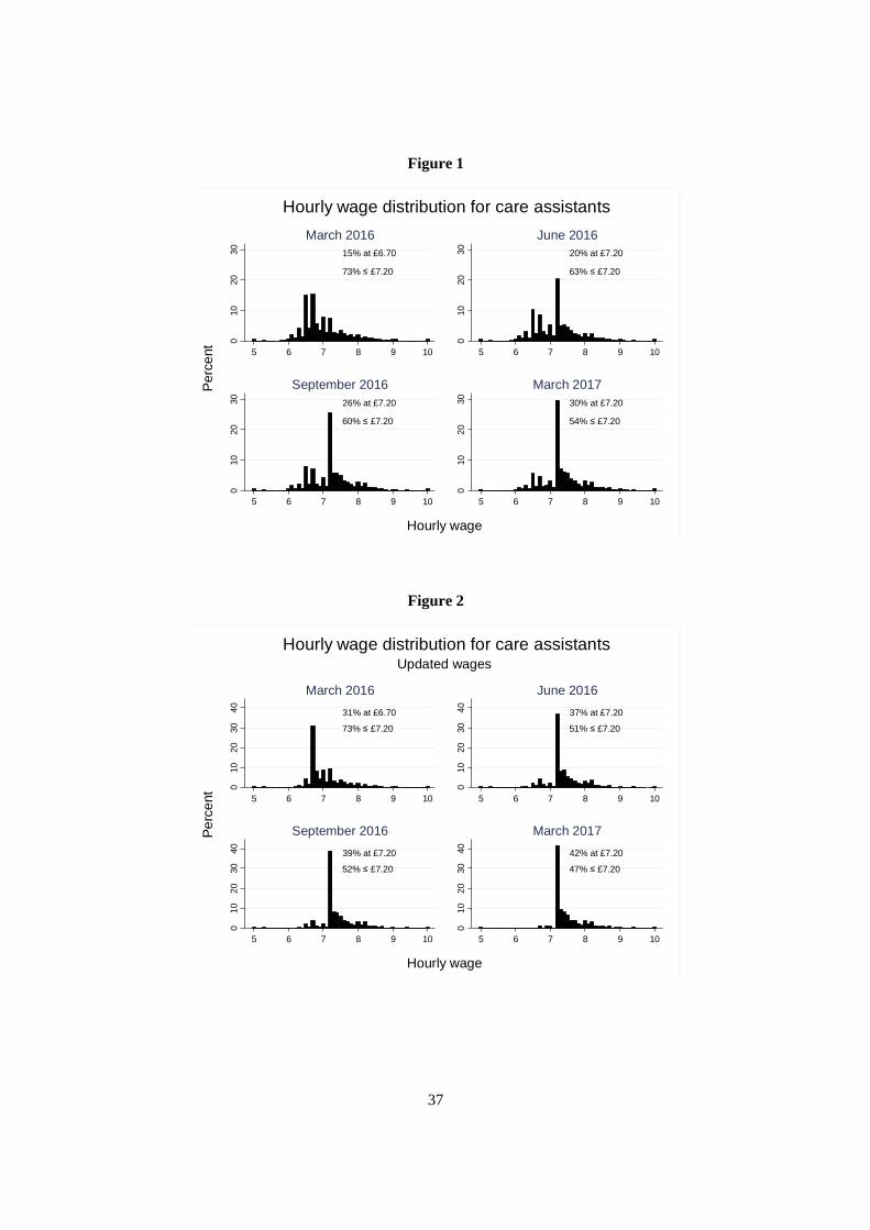
37

Figure 1

Figure 2

15% at £6.70

73% ≤ £7.20

010

2030

5 6 7 8 9 10

March 201620% at £7.20

63% ≤ £7.20

010

2030

5 6 7 8 9 10

June 2016

26% at £7.20

60% ≤ £7.20

010

2030

5 6 7 8 9 10

September 201630% at £7.20

54% ≤ £7.20

010

2030

5 6 7 8 9 10

March 2017Per

cent

Hourly wage

Hourly wage distribution for care assistants

31% at £6.70

73% ≤ £7.20

010

2030

40

5 6 7 8 9 10

March 2016

37% at £7.20

51% ≤ £7.20

010

2030

40

5 6 7 8 9 10

June 2016

39% at £7.20

52% ≤ £7.20

010

2030

40

5 6 7 8 9 10

September 2016

42% at £7.20

47% ≤ £7.20

010

2030

40

5 6 7 8 9 10

March 2017Per

cent

Hourly wage

Updated wagesHourly wage distribution for care assistants

38

Figure 3

Figure 4

20% at £6.70

82% ≤ £7.20

010

2030

5 6 7 8 9 10

March 201620% at £7.20

72% ≤ £7.20

010

2030

5 6 7 8 9 10

June 2016

25% at £7.20

69% ≤ £7.20

010

2030

5 6 7 8 9 10

September 201628% at £7.20

64% ≤ £7.20

010

2030

5 6 7 8 9 10

March 2017Per

cent

Hourly wage

Hourly wage distribution for care assistants under 25

34% at £6.70

81% ≤ £7.20

010

2030

40

5 6 7 8 9 10

March 201632% at £7.20

61% ≤ £7.20

010

2030

40

5 6 7 8 9 10

June 2016

33% at £7.20

63% ≤ £7.20

010

2030

40

5 6 7 8 9 10

September 201635% at £7.20

57% ≤ £7.20

010

2030

40

5 6 7 8 9 10

March 2017Per

cent

Hourly wage

Updated wagesHourly wage distribution for care assistants under 25

39

Figure 5

15% at £6.70

57% ≤ £7.20

010

2030

40

5 6 7 8 9 10

March 201634% at £7.20

45% ≤ £7.20

010

2030

40

5 6 7 8 9 10

June 2016

31% at £7.20

40% ≤ £7.20

010

2030

40

5 6 7 8 9 10

September 201629% at £7.20

33% ≤ £7.20

010

2030

40

5 6 7 8 9 10

March 2017Per

cent

Hourly wage

Updated wagesHourly wage distribution for domiciliary carers under 25

40

Table 1 – Descriptive Statistics

Mar 2016 Jun 2016 Sep 2016 Mar 2017 Mean S.D. Mean S.D. Mean S.D. Mean S.D.

Number of employees 38.93 30.94 39.21 31.27 39.35 31.77 39.58 31.29 Median 32.00 32.00 33.00 33.00 Proportion under 25 0.12 0.09 0.12 0.09 0.12 0.09 0.11 0.09 Wage 7.55 1.08 7.70 1.09 7.76 1.08 7.85 1.08 Wage (25 and over) 7.64 1.11 7.80 1.11 7.86 1.11 7.95 1.10 Wage (under 25) 6.82 0.78 6.97 0.81 7.03 0.80 7.11 0.80 Weekly hours 28.78 5.10 28.77 5.10 28.80 5.10 28.79 5.13 Weekly earnings 215.00 54.47 219.15 55.35 221.30 55.45 223.92 56.12 Proportion female 0.84 0.13 0.84 0.13 0.84 0.13 0.84 0.13 Age 42.69 4.60 42.74 4.58 42.82 4.61 43.04 4.63 Proportion care assistant 0.56 0.16 0.56 0.16 0.56 0.16 0.56 0.16 Proportion with nursing qualification

0.04 0.07 0.04 0.07 0.04 0.07 0.04 0.07

Occupancy rate 0.92 0.15 0.92 0.14 0.92 0.14 0.92 0.14 Number of homes 4,134 4,134 4,134 4,134

Notes: The sample is a balanced panel of homes active between March 2016 and March 2017.

Table 2 – The Bite of the National Living Wage

Mar 2016 Jun 2016 Sep 2016 Mar 2017 Mean S.D. Mean S.D. Mean S.D. Mean S.D.

Proportion paid less than minimum wage 0.51 0.32 0.35 0.35 0.29 0.33 0.22 0.30 Proportion paid less than minimum wage (25 and over)

0.55 0.34 0.37 0.37 0.30 0.35 0.23 0.31

NLW gap 0.04 0.04 0.03 0.04 0.02 0.04 0.02 0.03 NLW gap (25 and over) 0.04 0.04 0.03 0.04 0.02 0.03 0.02 0.03 Proportion paid exactly £7.20 0.03 0.10 0.13 0.23 0.17 0.25 0.20 0.26 Proportion paid exactly £7.20 (25 and over) 0.03 0.10 0.13 0.23 0.17 0.26 0.20 0.27

Notes: The sample is a balanced panel of homes active between March 2016 and March 2017.

41

Table 3 – Wage Equations

Dep. Var.: Change in log average hourly wage

Panel A – March 2016 to June 2016

(1) (2) (3) (4) Initial low-paid proportion 0.023*** 0.021***

(0.002) (0.002) Initial NLW gap 0.136*** 0.110***

(0.018) (0.019)

Observations 4,134 4,134 4,134 4,134 Controls No Yes No Yes

Panel B – March 2016 to September 2016

(1) (2) (3) (4) Initial low-paid proportion 0.037*** 0.036***

(0.002) (0.002) Initial NLW gap 0.264*** 0.244***

(0.023) (0.026)

Observations 4,134 4,134 4,134 4,134 Controls No Yes No Yes

Panel C – March 2016 to March 2017

(1) (2) (3) (4) Initial low-paid proportion 0.049*** 0.049***

(0.002) (0.002) Initial NLW gap 0.400*** 0.390***

(0.027) (0.029)

Observations 4,134 4,134 4,134 4,134 Controls No Yes No Yes

Notes: The sample is a balanced panel of homes active between March 2016 and March 2017. Robust standard errors are reported in parentheses. P-value: *** p<0.01, ** p<0.05, * p<0.1. Control variables are the initial proportion female, proportion with nursing qualification, proportion of care assistants, average age (all workers), occupancy rate and regional dummies.

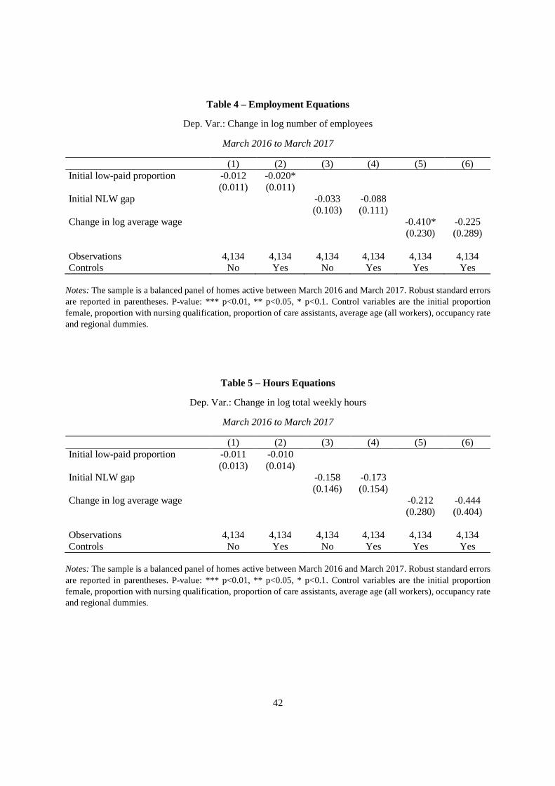
42

Table 4 – Employment Equations

Dep. Var.: Change in log number of employees

March 2016 to March 2017

(1) (2) (3) (4) (5) (6) Initial low-paid proportion -0.012 -0.020*

(0.011) (0.011) Initial NLW gap -0.033 -0.088

(0.103) (0.111) Change in log average wage -0.410* -0.225

(0.230) (0.289)

Observations 4,134 4,134 4,134 4,134 4,134 4,134 Controls No Yes No Yes Yes Yes

Notes: The sample is a balanced panel of homes active between March 2016 and March 2017. Robust standard errors are reported in parentheses. P-value: *** p<0.01, ** p<0.05, * p<0.1. Control variables are the initial proportion female, proportion with nursing qualification, proportion of care assistants, average age (all workers), occupancy rate and regional dummies.

Table 5 – Hours Equations

Dep. Var.: Change in log total weekly hours

March 2016 to March 2017

(1) (2) (3) (4) (5) (6) Initial low-paid proportion -0.011 -0.010

(0.013) (0.014) Initial NLW gap -0.158 -0.173

(0.146) (0.154) Change in log average wage -0.212 -0.444

(0.280) (0.404)

Observations 4,134 4,134 4,134 4,134 4,134 4,134 Controls No Yes No Yes Yes Yes

Notes: The sample is a balanced panel of homes active between March 2016 and March 2017. Robust standard errors are reported in parentheses. P-value: *** p<0.01, ** p<0.05, * p<0.1. Control variables are the initial proportion female, proportion with nursing qualification, proportion of care assistants, average age (all workers), occupancy rate and regional dummies.

43

Table 6 – Wage Spillover Equations

Dep. Var.: Change in log average hourly wage for employees aged under 25

Panel A – March 2016 to June 2016

IV Proport. below

IV NLW gap

(1) (2) (3) (4) (5) (6) Initial low-paid proportion (25+) 0.017*** 0.017***

(0.003) (0.003) Initial NLW gap (25+) 0.109*** 0.110***

(0.031) (0.033) Change in log average wage (25+) 0.643*** 0.592***

(0.103) (0.152)

Observations 2,866 2,866 2,866 2,866 2,866 2,866 Controls No Yes No Yes Yes Yes

Panel B – March 2016 to September 2016

(1) (2) (3) (4) (5) (6) Initial low-paid proportion (25+) 0.029*** 0.031***

(0.004) (0.004) Initial NLW gap (25+) 0.220*** 0.234***

(0.040) (0.043) Change in log average wage (25+)

0.747*** 0.724***

(0.089) (0.118)

Observations 2,866 2,866 2,866 2,866 2,866 2,866 Controls No Yes No Yes Yes Yes

Panel C – March 2016 to March 2017

(1) (2) (3) (4) (5) (6) Initial low-paid proportion (25+) 0.033*** 0.038***

(0.005) (0.005) Initial NLW gap (25+) 0.268*** 0.308***

(0.060) (0.063) Change in log average wage (25+) 0.722*** 0.654***

(0.100) (0.125)

Observations 2,866 2,866 2,866 2,866 2,866 2,866 Controls No Yes No Yes Yes Yes

Notes: The sample is a balanced panel of homes active between March 2016 and March 2017. Robust standard errors are reported in parentheses. P-value: *** p<0.01, ** p<0.05, * p<0.1. Control variables are the initial proportion female, proportion with nursing qualification, proportion of care assistants, average age (all workers), occupancy rate and regional dummies.

44

Table 7 – Employment Spillover Equations

Dep. Var.: Change in share of employees aged under 25

March 2016 to March 2017

(1) (2) (3) (4) (5) (6) Initial low-paid proportion (25+) -0.004 -0.001

(0.004) (0.004) Initial NLW gap (25+) -0.002 0.007

(0.034) (0.038) Change in log average wage (25+) -0.026 0.014

(0.075) (0.080)

Observations 2,866 2,866 2,866 2,866 2,866 2,866 Controls No Yes No Yes Yes Yes

Notes: The sample is a balanced panel of homes active between March 2016 and March 2017. Robust standard errors are reported in parentheses. P-value: *** p<0.01, ** p<0.05, * p<0.1. Control variables are the initial proportion female, proportion with nursing qualification, proportion of care assistants, average age (all workers), occupancy rate and regional dummies.

Table 8 – Total Hours Spillover Equations

Dep. Var.: Change in share of total weekly hours worked by employees aged under 25

March 2016 to March 2017

(1) (2) (3) (4) (5) (6) Initial low-paid proportion (25+) -0.002 0.001

(0.004) (0.004) Initial NLW gap (25+) 0.009 0.020

(0.036) (0.040) Change in log average wage (25+) 0.022 0.042

(0.078) (0.084)

Observations 2,866 2,866 2,866 2,866 2,866 2,866 Controls No Yes No Yes Yes Yes

Notes: The sample is a balanced panel of homes active between March 2016 and March 2017. Robust standard errors are reported in parentheses. P-value: *** p<0.01, ** p<0.05, * p<0.1. Control variables are the initial proportion female, proportion with nursing qualification, proportion of care assistants, average age (all workers), occupancy rate and regional dummies.

45

Table 9 –Differences between the Care Home and the Domiciliary Care Sector

March 2016

Care Homes Domiciliary Care Difference

Mean S.D. Mean S.D.

Firm-level outcomes

Number of employees 38.93 30.94 62.90 70.52 -23.97 ***

Proportion under 25 0.12 0.09 0.12 0.09 0.01 *

Number of firms 4,134 1,248

Worker-level outcomes

Wage 7.65 2.07 7.52 1.25 0.13 ***

Wage (under 25) 6.85 1.10 7.25 0.79 -0.41 ***

Proportion on zero-hour contracts 0.07 0.25 0.64 0.48 -0.57 ***

Proportion on zero-hour contracts (under 25) 0.12 0.33 0.67 0.47 -0.54 ***

Proportion on permanent contracts 0.90 0.29 0.83 0.38 0.08 ***

Proportion on temporary contracts 0.01 0.12 0.05 0.23 -0.04 ***

Proportion bank workers 0.07 0.26 0.04 0.20 0.03 ***

Proportion agency workers 0.00 0.04 0.05 0.23 -0.05 ***

Weekly hours 28.43 11.80 12.27 15.89 16.16 ***

Weekly earnings 215.45 118.30 74.44 118.79 141.01 ***

Proportion female 0.84 0.37 0.87 0.34 -0.02 ***

Age 42.31 13.92 41.65 13.39 0.65 ***

Proportion care assistant 0.55 0.50 0.81 0.39 -0.26 ***

Proportion with nursing qualification 0.05 0.23 0.00 0.05 0.05 ***

Number of workers 181,888 131,680

Notes: The sample is made of all workers and firms in the balanced panel of care homes and domiciliary care agencies active between March 2016 and March 2017. The last column reports the difference in means between the care home and domiciliary care sectors and the associated significance level. P-value: *** p<0.01, ** p<0.05, * p<0.1.

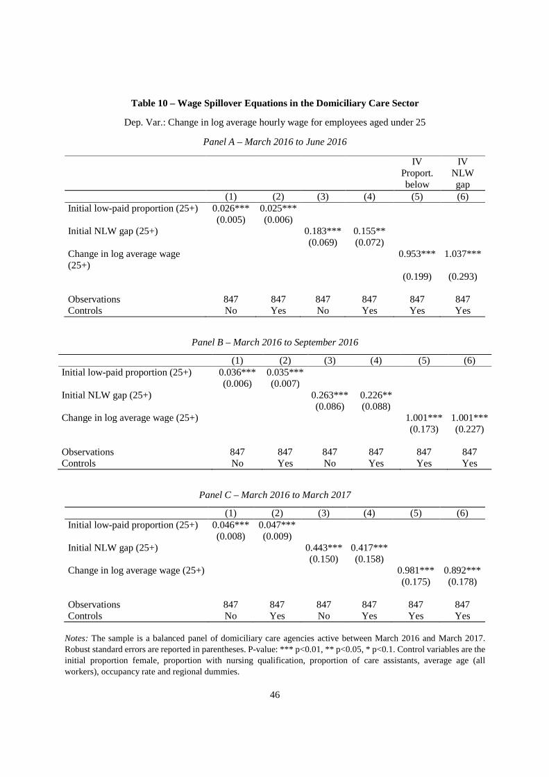
46

Table 10 – Wage Spillover Equations in the Domiciliary Care Sector

Dep. Var.: Change in log average hourly wage for employees aged under 25

Panel A – March 2016 to June 2016

IV Proport. below

IV NLW gap

(1) (2) (3) (4) (5) (6) Initial low-paid proportion (25+) 0.026*** 0.025***

(0.005) (0.006) Initial NLW gap (25+) 0.183*** 0.155**

(0.069) (0.072) Change in log average wage (25+)

0.953*** 1.037***

(0.199) (0.293)

Observations 847 847 847 847 847 847 Controls No Yes No Yes Yes Yes

Panel B – March 2016 to September 2016

(1) (2) (3) (4) (5) (6) Initial low-paid proportion (25+) 0.036*** 0.035***

(0.006) (0.007) Initial NLW gap (25+) 0.263*** 0.226**

(0.086) (0.088) Change in log average wage (25+) 1.001*** 1.001***

(0.173) (0.227)

Observations 847 847 847 847 847 847 Controls No Yes No Yes Yes Yes

Panel C – March 2016 to March 2017

(1) (2) (3) (4) (5) (6) Initial low-paid proportion (25+) 0.046*** 0.047***

(0.008) (0.009) Initial NLW gap (25+) 0.443*** 0.417***

(0.150) (0.158) Change in log average wage (25+) 0.981*** 0.892***

(0.175) (0.178)

Observations 847 847 847 847 847 847 Controls No Yes No Yes Yes Yes

Notes: The sample is a balanced panel of domiciliary care agencies active between March 2016 and March 2017. Robust standard errors are reported in parentheses. P-value: *** p<0.01, ** p<0.05, * p<0.1. Control variables are the initial proportion female, proportion with nursing qualification, proportion of care assistants, average age (all workers), occupancy rate and regional dummies.

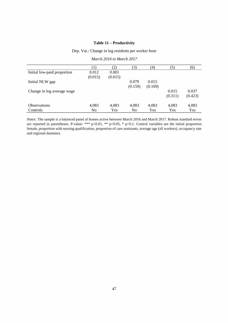
47

Table 11 – Productivity

Dep. Var.: Change in log residents per worker hour

March 2016 to March 2017

(1) (2) (3) (4) (5) (6) Initial low-paid proportion 0.012 0.001

(0.015) (0.015) Initial NLW gap 0.079 0.015

(0.159) (0.169) Change in log average wage 0.015 0.037

(0.311) (0.423)

Observations 4,083 4,083 4,083 4,083 4,083 4,083 Controls No Yes No Yes Yes Yes

Notes: The sample is a balanced panel of homes active between March 2016 and March 2017. Robust standard errors are reported in parentheses. P-value: *** p<0.01, ** p<0.05, * p<0.1. Control variables are the initial proportion female, proportion with nursing qualification, proportion of care assistants, average age (all workers), occupancy rate and regional dummies.

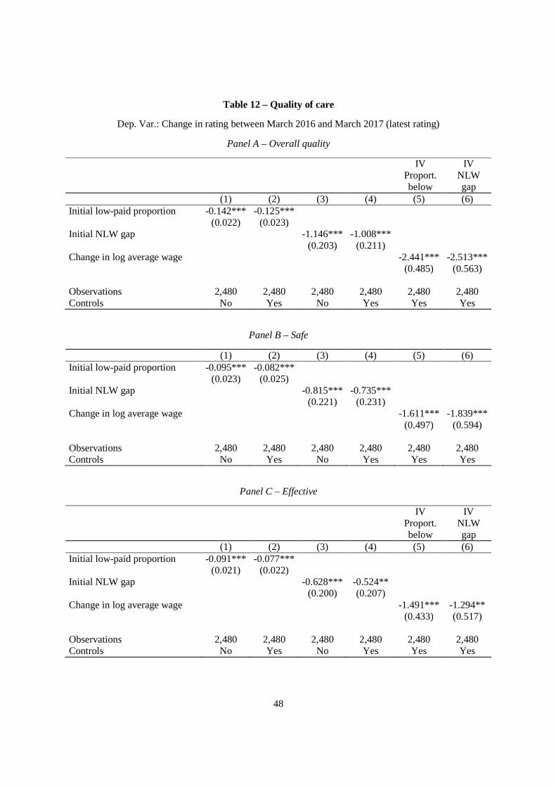
48

Table 12 – Quality of care

Dep. Var.: Change in rating between March 2016 and March 2017 (latest rating)

Panel A – Overall quality

IV Proport. below

IV NLW gap

(1) (2) (3) (4) (5) (6) Initial low-paid proportion -0.142*** -0.125***

(0.022) (0.023) Initial NLW gap -1.146*** -1.008***

(0.203) (0.211) Change in log average wage -2.441*** -2.513***

(0.485) (0.563)

Observations 2,480 2,480 2,480 2,480 2,480 2,480 Controls No Yes No Yes Yes Yes

Panel B – Safe

(1) (2) (3) (4) (5) (6) Initial low-paid proportion -0.095*** -0.082***

(0.023) (0.025) Initial NLW gap -0.815*** -0.735***

(0.221) (0.231) Change in log average wage -1.611*** -1.839***

(0.497) (0.594)

Observations 2,480 2,480 2,480 2,480 2,480 2,480 Controls No Yes No Yes Yes Yes

Panel C – Effective

IV Proport. below

IV NLW gap

(1) (2) (3) (4) (5) (6) Initial low-paid proportion -0.091*** -0.077***

(0.021) (0.022) Initial NLW gap -0.628*** -0.524**

(0.200) (0.207) Change in log average wage -1.491*** -1.294**

(0.433) (0.517)

Observations 2,480 2,480 2,480 2,480 2,480 2,480 Controls No Yes No Yes Yes Yes

49

Panel D – Caring

(1) (2) (3) (4) (5) (6) Initial low-paid proportion -0.078*** -0.077***

(0.015) (0.016) Initial NLW gap -0.520*** -0.506***

(0.150) (0.156) Change in log average wage -1.512*** -1.266***

(0.335) (0.404)

Observations 2,480 2,480 2,480 2,480 2,480 2,480 Controls No Yes No Yes Yes Yes

Panel E – Responsive

(1) (2) (3) (4) (5) (6) Initial low-paid proportion -0.091*** -0.075***

(0.020) (0.021) Initial NLW gap -0.795*** -0.697***

(0.194) (0.200) Change in log average wage -1.460*** -1.727***

(0.423) (0.517)

Observations 2,480 2,480 2,480 2,480 2,480 2,480 Controls No Yes No Yes Yes Yes

Panel F – Well-led

(1) (2) (3) (4) (5) (6) Initial low-paid proportion -0.124*** -0.110***

(0.024) (0.026) Initial NLW gap -0.997*** -0.883***

(0.226) (0.236) Change in log average wage -2.150*** -2.202***

(0.521) (0.604)

Observations 2,480 2,480 2,480 2,480 2,480 2,480 Controls No Yes No Yes Yes Yes

Notes: The sample is a balanced panel of homes active between March 2016 and March 2017. Robust standard errors are reported in parentheses. P-value: *** p<0.01, ** p<0.05, * p<0.1. Control variables are the latest rating in the relevant line of enquiry as of March 2016, the initial proportion female, proportion with nursing qualification, proportion of care assistants, average age (all workers), occupancy rate and regional dummies.

50

Table 13 – Closures

Dep. Var.: Indicator for Firm Closure

March 2016 to March 2017

(1) (2) (3) (4) Initial low-paid proportion -0.001 0.003

(0.007) (0.007) Initial NLW gap 0.038 0.066

(0.059) (0.062)

Observations 4,306 4,306 4,306 4,306 Controls No Yes No Yes

Notes: The sample is a balanced panel of homes active in March 2016, unconditional on their survival until March 2017. Robust standard errors are reported in parentheses. P-value: *** p<0.01, ** p<0.05, * p<0.1. Control variables are the initial proportion female, proportion with nursing qualification, proportion of care assistants, average age (all workers), occupancy rate and regional dummies.

51

Appendix A1 – Aggregate employment and firm dynamics

A1.1 Aggregate Employment Effects

We explore the aggregate employment effects of the NLW introduction using a bunching approach as in

Cengiz et al. (2018). The bunching approach allows us to infer the effect on employment throughout the

wage distribution by comparing the number of missing jobs below the minimum to the number of excess

jobs above the minimum before and after the policy change. The main intuition behind this approach is that

when a higher minimum wage is introduced, workers who used to be paid at a wage below the new

minimum can no longer be paid at their old rate. As a consequence, provided that there is almost full

compliance with the law, the mass of jobs at the bottom of the wage distribution should disappear. Some

of these jobs will obtain the wage uprate and therefore appear at or right above the new minimum, some

might be destroyed, and some other new jobs might be created through a labour supply effect. Therefore,

the size of the excess mass above the new minimum provides an account of preserved and newly created

jobs, and the sum of the excess and the missing mass measures the total employment change, whether

positive or negative. It is reasonable to believe that the bulk of the dynamics will occur in a neighbourhood

of the new minimum, as changes in the upper tail of the wage distribution are unlikely to be driven by

minimum wage changes.

To implement this strategy, we consider the entire workforce of care homes ever active between

October 2015 and March 2017, therefore allowing for entries and exits. This allows us to investigate the

aggregate employment effects of the NLW introduction. We collapse the individual data and calculate

monthly employment counts at the local authority district level by £0.50 hourly wage bins from six months

prior to a year after the NLW introduction, and from two pounds below to five pounds above the NLW rate

of £7.20.36 We then estimate how changes in the excess and missing mass by wage bin evolve relative to

March 2016 adopting the following fixed effect framework:

36 While we do not have any ex-ante information on what is the range over which the minimum wage change can have distributional consequences, we draw on the information in Figure 1 and restrict our analysis to wages between £5.20 and £11.20.

52

!3,4,� = %5 + 6 6 %7,8947 × 9�8�)

8;"�,8<"1

=

7<">+ ?3,4,� (7)

where !3,4,� is employment headcount in local authority �, wage bin @ and month A, 947 is an indicator

taking value one if wage bin @ is B-bin distant from the £7.20 bin, 9�8 is an indicator taking value one if

month A is C-period distant from April 2016 and ?3,4,� a disturbance term. The key parameters of interest

are %7,8 for B = {−4, … , 8} and C = {−6, −5, … , −2, 0, … , 11,12}, as they trace the evolution of the missing

and excess mass relative to the time of the policy change. In this model, given that the timing of the NLW

introduction is common to all local authorities, identification comes from variation in the number of

workers for which the minimum wage change is binding across local authorities.

In Figure A5 in Appendix A2 the vertical bars correspond to the estimated %87 for B = {−4, … ,8}and for selected values of C, namely C = 3 in the top left panel, C = 6 in the top right panel, C = 9 in the

bottom left panel and C = 12 in the bottom right panel. For each bar, a capped line indicates the 95 percent

confidence interval of the %M87. The connected dots indicate instead the cumulative sum of the bin-specific

effects. Across all the panels, the missing mass is concentrated in the two wage bins right below the new

minimum and the excess mass in the first bin above it, while employment changes in the other bins are very

small and statistically indistinguishable from zero. The pattern of the cumulated effects suggests that jobs

previously paid below the NLW are fully replaced by jobs in the three bins right above the new minimum,

and that there are no spillover effects in the upper part of the wage distribution.

While the previous chart displays the change in mass by wage bin for selected post-treatment

periods relative to March 2016, Figure A6 in Appendix A2 documents the evolution of the total number of

jobs below the minimum �8 = ∑ %87"�7<"> (missing mass), the total number of jobs above the minimum �8 =

∑ %87=7<5 (excess mass), and their sum Δ8 = �8 + �8 (net excess mass) for C ={−6, −5, … , −2, 0, … , 11,12}. The numbers reported at the bottom of the figure are the point estimates

ΔN8. The graph shows a sharp reduction in the number of jobs below the NLW between the six months prior

and the twelve months after its implementation. The below mass decreases by a statistically significant

53

amount exactly in April 2016 – showing that the minimum wage increase had real bite – and remains

persistently negative throughout the following twelve months. The evolution of the excess mass almost

perfectly mirrors this pattern, displaying a significant and positive jump from C = 0 onwards. This is

confirmed by the behaviour of the “net excess mass” that is very small in magnitude and never statistically

different from zero. Interestingly enough, there is no pre-trend in �M8 nor �P8. According to these result, there

is little if no indication of negative aggregate employment effects due to the NLW introduction.

Following our previous investigation of potential spillover effects, we extend the bunching

framework to account for different patterns between workers aged under 25, and workers aged 25 and over.

In practice, we augment the bunching model interacting the main regressor with an age-group dummy.37

Results are reported in Figures A7 and A8 in Appendix A2 for adult workers, and in Figures A9 and A10

for younger workers. The age-specific patterns are very similar to the aggregate ones. The evolution of the

net excess mass in Figure A10 seems to suggest a mild but nonetheless small and statistically insignificant

negative employment effect for younger workers. All in all, we take this bunching exercise as evidence that

the NLW introduction did not have any significant aggregate employment effects.

A1.2 Aggregate firm dynamics

We are also interested in whether the NLW introduction had an impact on firm entry. We therefore

consider all firms ever active in the period between March 2016 and March 2017, allowing for both entries

into and exits out of the sample. Estimating reduced-form linear probability models for the probability of

entry as we did above for the probability of exit is infeasible, since we do not have a measure of the

minimum wage bite for entrants. We therefore collapse the data at the local authority district level38 and

run reduced-form regressions of the following form:

Q3,� = �> + �>� !3,�"� + R3,�"�$ %> + S3,� (8)

37 This model requires collapsing the data by age category, wage bin, month and local authority. 38 Local authority district areas as defined by ONS split England into 326 areas of local governance.

54

where Q3,� is the proportion of entrants in local authority � between March 2016 and time T – where T can

be June 2016, September 2016 or March 2017 – , � !3,�"�is either the proportion of low-paid workers or

the wage gap at local authority level in March 2016, and R is a vector of local-authority controls including

the proportion of female workers, average age, the proportion working as care assistants, the proportion

with nursing qualification, the occupancy rate and a set of regional dummies. For entries between March

2016 and March 2017, reduced form estimates are reported in columns (1) to (4) of Panel C of Table A16

in Appendix A2. Columns (5) and (6) instead show structural form estimates in which � !3,�"� is used as

an instrument for the change in the logarithm of the average wage in the local authority ���3,�.39 The

statistical insignificance of the estimated coefficients and their limited size indicate that the NLW

introduction did not have an impact on firm entry at the local authority level.

For completeness, we also report reduced-form and structural-form estimates for firm exits at the

local authority level in Table A17 in Appendix A2. Consistently with the firm-level results, we do not find

evidence of a detrimental effect of the NLW introduction on care home survival.

39 Estimates for entries between March and June 2016 are reported in Panel A of Table A16 in Appendix A2, while those for entries between March and September 2016 in Panel B of the same table.

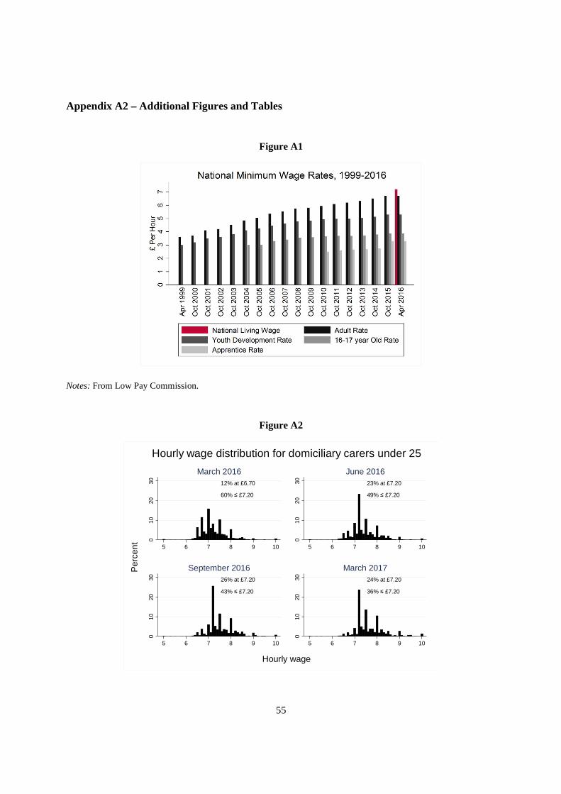
55

Appendix A2 – Additional Figures and Tables

Figure A1

Notes: From Low Pay Commission.

Figure A2

12% at £6.70

60% ≤ £7.20

010

2030

5 6 7 8 9 10

March 201623% at £7.20

49% ≤ £7.20

010

2030

5 6 7 8 9 10

June 2016

26% at £7.20

43% ≤ £7.20

010

2030

5 6 7 8 9 10

September 201624% at £7.20

36% ≤ £7.20

010

2030

5 6 7 8 9 10

March 2017Per

cent

Hourly wage

Hourly wage distribution for domiciliary carers under 25

56

Figure A3

Notes: Panel A is based on the sample of 2480 homes with CQC ratings as of March 2016. Panel B is based on the subgroup of firms that were inspected and rated by CQC both before and after March 2016. Legend: 1 = inadequate, 2 = requires improvement, 3 = good, 4 = outstanding.

Figure A4

Notes: Panel A is based on the sample of 2480 homes with CQC ratings as of March 2016. Panel B is based on the subgroup of firms that were inspected and rated by CQC both before and after March 2016.

020

4060

8010

0

1 2 3 4

Overall0

2040

6080

100

1 2 3 4

Safe

020

4060

8010

01 2 3 4

Effective

020

4060

8010

0

1 2 3 4

Caring

020

4060

8010

0

1 2 3 4

Responsive

020

4060

8010

0

1 2 3 4

Well-ledPer

cent

Rating

Panel A

020

4060

8010

0

1 2 3 4

Overall

020

4060

8010

0

1 2 3 4

Safe

020

4060

8010

0

1 2 3 4

Effective

020

4060

8010

0

1 2 3 4

Caring

020

4060

8010

0

1 2 3 4

Responsive

020

4060

8010

0

1 2 3 4

Well-ledPer

cent

Rating

Panel B

Distribution of ratings in March 2016

020

4060

8010

0

-2 -1 0 1 2

Overall

020

4060

8010

0

-2 -1 0 1 2

Safe

020

4060

8010

0

-2 -1 0 1 2

Effective

020

4060

801

00

-2 -1 0 1 2

Caring

020

4060

801

00

-2 -1 0 1 2

Responsive

020

4060

801

00

-2 -1 0 1 2

Well-ledPer

cent

Change in rating

Panel A

020

4060

8010

0

-2 -1 0 1 2

Overall

020

4060

8010

0

-2 -1 0 1 2

Safe

020

4060

8010

0

-2 -1 0 1 2

Effective

020

4060

801

00

-2 -1 0 1 2

Caring

020

4060

801

00

-2 -1 0 1 2

Responsive

020

4060

801

00

-2 -1 0 1 2

Well-ledPer

cent

Change in rating

Panel B

Distribution of change in ratings between March 2016 and March 2017

57

Figure A5

Notes: The vertical bars correspond to the estimated %87 from equation (7) for wage bins B = {−4, … ,8} and for C = 3in the top left panel, C = 6 in the top right panel, C = 9 in the bottom left panel and C = 12 in the bottom right panel.Capped lines indicate 95 percent confidence intervals, computed using robust standard errors. The connected dots indicate the cumulative sum of the bin-specific effects.

Figure A6

Notes: Missing mass is the total number of jobs below the minimum �8 = ∑ %87"�7<"> , excess mass the total number ofjobs above the minimum �8 = ∑ %87=7<5 , net excess mass the sum ΔU = �8 + �8. Coefficient estimates of the net excessmass are reported in grey at the bottom of the figure. Vertical bars indicate 95 percent confidence intervals, computed using robust standard errors.

-200

-100

010

020

0

-4 -2 0 2 4 6 8

June 2016

-200

-100

010

020

0

-4 -2 0 2 4 6 8

September 2016

-200

-100

010

020

0

-4 -2 0 2 4 6 8

December 2016

-200

-100

010

020

0-4 -2 0 2 4 6 8

March 2017

Ave

rage

em

ploy

men

t by

loca

l aut

horit

y

Wage bin (£0.50) relative to NLW

Change in employment by wage bin relative to March 2016

-4.3 -4 -3.9 -2.5 -2.6 -2.4 0 2.4 6 7.4 8.2 7.3 7.9 8.5 6.7 7 6.2 4.7 5.4

-200

-100

010

020

0A

vera

ge e

mpl

oym

ent b

y lo

cal a

utho

rity

2015

m9

2015

m12

2016

m3

2016

m6

2016

m9

2016

m12

2017

m3

Missing mass Excess mass Net exc. mass

Evolution of missing and excess mass

58

Figure A7

Notes: The vertical bars correspond to the estimated %87 from equation (7) for wage bins B = {−4, … ,8} and for C = 3in the top left panel, C = 6 in the top right panel, C = 9 in the bottom left panel and C = 12 in the bottom right panel.Capped lines indicate 95 percent confidence intervals, computed using robust standard errors. The connected dots indicate the cumulative sum of the bin-specific effects.

Figure A8

Notes: Missing mass is the total number of jobs below the minimum �8 = ∑ %87"�7<"> , excess mass the total number ofjobs above the minimum �8 = ∑ %87=7<5 , net excess mass the sum ΔU = �8 + �8. Coefficient estimates of the net excessmass are reported in grey at the bottom of the figure. Vertical bars indicate 95 percent confidence intervals, computed using robust standard errors.

-100

-50

050

100

-4 -2 0 2 4 6 8

June 2016

-100

-50

050

100

-4 -2 0 2 4 6 8

September 2016-1

00-5

00

5010

0

-4 -2 0 2 4 6 8

December 2016

-100

-50

050

100

-4 -2 0 2 4 6 8

March 2017

Ave

rage

em

ploy

men

t by

loca

l aut

horit

y

Wage bin (£0.50) relative to NLW

Employees aged 25 and overChange in employment by wage bin relative to March 2016

-8.7 -7 -5.8 -4.2 -3.2 -1.8 0 -.2 2.8 3.9 5.4 5.2 6.7 8 7.4 8.1 7.4 6.9 7.2

-200

-100

010

020

0A

vera

ge e

mpl

oym

ent b

y lo

cal a

utho

rity

2015

m9

2015

m12

2016

m3

2016

m6

2016

m9

2016

m12

2017

m3

Missing mass Excess mass Net exc. mass

Employees aged 25 and overEvolution of missing and excess mass

59

Figure A9

Notes: The vertical bars correspond to the estimated %87 from equation (7) for wage bins B = {−4, … ,8} and for C = 3in the top left panel, C = 6 in the top right panel, C = 9 in the bottom left panel and C = 12 in the bottom right panel.Capped lines indicate 95 percent confidence intervals, computed using robust standard errors. The connected dots indicate the cumulative sum of the bin-specific effects.

Figure A10

Notes: Missing mass is the total number of jobs below the minimum �8 = ∑ %87"�7<"> , excess mass the total numberof jobs above the minimum �8 = ∑ %87=7<5 , net excess mass the sum ΔU = �8 + �8. Coefficient estimates of the netexcess mass are reported in grey at the bottom of the figure. Vertical bars indicate 95 percent confidence intervals, computed using robust standard errors.

-20

-10

010

20

-4 -2 0 2 4 6 8

June 2016

-20

-10

010

20

-4 -2 0 2 4 6 8

September 2016-2

0-1

00

1020

-4 -2 0 2 4 6 8

December 2016

-20

-10

010

20-4 -2 0 2 4 6 8

March 2017

Ave

rage

em

ploy

men

t by

loca

l aut

horit

y

Wage bin (£0.50) relative to NLW

Employees aged under 25Change in employment by wage bin relative to March 2016

4 2.6 1.7 1.3 .6 -.5 0 1.1 .9 1.3 .6 -.1 -1 -1.6 -2.6 -3.3 -3.5 -4.1 -4

-30

-20

-10

010

20A

vera

ge e

mpl

oym

ent b

y lo

cal a

utho

rity

2015

m9

2015

m12

2016

m3

2016

m6

2016

m9

2016

m12

2017

m3

Missing mass Excess mass Net exc. mass

Employees aged under 25Evolution of missing and excess mass

60

Table A1 – Identification Checks

Panel A – Dep. Var.: Change in log average hourly wage

March to June March to September 2015 2016 Difference 2015 2016 Difference (1) (2) (3) (4) (5) (6)

Initial log average hourly wage -0.016*** -0.060*** -0.043*** -0.032*** -0.099*** -0.067*** (0.003) (0.006) (0.007) (0.005) (0.009) (0.010)

Observations 4,126 4,134 8,260 4,126 4,134 8,260

Panel B – Dep. Var.: Change in log number of employees

March to June March to September 2015 2016 Difference 2015 2016 Difference (1) (2) (3) (4) (5) (6)

Initial log average hourly wage -0.000 0.030* 0.031 -0.007 -0.002 0.004 (0.018) (0.017) (0.024) (0.024) (0.024) (0.033)

Observations 4,126 4,134 8,260 4,126 4,134 8,260

Panel C – Dep. Var.: Change in log total weekly hours

March to June March to September 2015 2016 Difference 2015 2016 Difference (1) (2) (3) (4) (5) (6)

Initial log average hourly wage 0.009 0.037 0.028 0.013 -0.007 -0.020 (0.019) (0.023) (0.030) (0.026) (0.029) (0.039)

Observations 4,126 4,134 8,260 4,126 4,134 8,260

Notes: The sample in columns (1) and (4) is a balanced panel of homes active between March 2015 and March 2016. The sample in columns (2) and (5) is a balanced panel of homes active between March 2016 and March 2017. Columns (3) and (5) are based on both samples. Robust standard errors are reported in parentheses. P-value: *** p<0.01, ** p<0.05, * p<0.1.

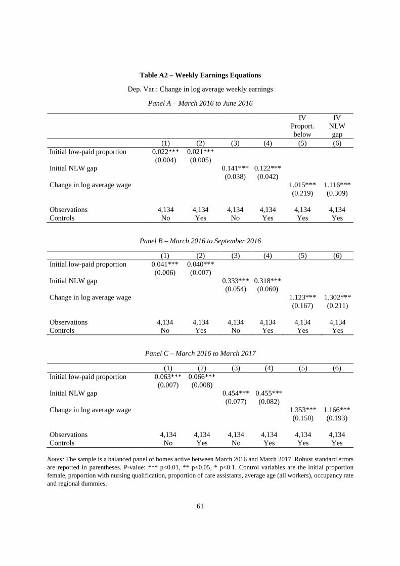
61

Table A2 – Weekly Earnings Equations

Dep. Var.: Change in log average weekly earnings

Panel A – March 2016 to June 2016

IV Proport. below

IV NLW gap

(1) (2) (3) (4) (5) (6) Initial low-paid proportion 0.022*** 0.021***

(0.004) (0.005) Initial NLW gap 0.141*** 0.122***

(0.038) (0.042) Change in log average wage 1.015*** 1.116***

(0.219) (0.309)

Observations 4,134 4,134 4,134 4,134 4,134 4,134 Controls No Yes No Yes Yes Yes

Panel B – March 2016 to September 2016

(1) (2) (3) (4) (5) (6) Initial low-paid proportion 0.041*** 0.040***

(0.006) (0.007) Initial NLW gap 0.333*** 0.318***

(0.054) (0.060) Change in log average wage 1.123*** 1.302***

(0.167) (0.211)

Observations 4,134 4,134 4,134 4,134 4,134 4,134 Controls No Yes No Yes Yes Yes

Panel C – March 2016 to March 2017

(1) (2) (3) (4) (5) (6) Initial low-paid proportion 0.063*** 0.066***

(0.007) (0.008) Initial NLW gap 0.454*** 0.455***

(0.077) (0.082) Change in log average wage 1.353*** 1.166***

(0.150) (0.193)

Observations 4,134 4,134 4,134 4,134 4,134 4,134 Controls No Yes No Yes Yes Yes

Notes: The sample is a balanced panel of homes active between March 2016 and March 2017. Robust standard errors are reported in parentheses. P-value: *** p<0.01, ** p<0.05, * p<0.1. Control variables are the initial proportion female, proportion with nursing qualification, proportion of care assistants, average age (all workers), occupancy rate and regional dummies.

62

Table A3 – Employment Equations

Dep. Var.: Change in log number of employees

Panel A – March 2016 to June 2016

IV Proport. below

IV NLW gap

(1) (2) (3) (4) (5) (6) Initial low-paid proportion -0.011* -0.014**

(0.006) (0.007) Initial NLW gap -0.104 -0.127*

(0.065) (0.068) Change in log average wage -0.661** -1.157*

(0.325) (0.676)

Observations 4,134 4,134 4,134 4,134 4,134 4,134 Controls No Yes No Yes Yes Yes

Panel B – March 2016 to September 2016

(1) (2) (3) (4) (5) (6) Initial low-paid proportion -0.011 -0.016*

(0.008) (0.009) Initial NLW gap -0.048 -0.086

(0.087) (0.094) Change in log average wage -0.460* -0.354

(0.246) (0.395)

Observations 4,134 4,134 4,134 4,134 4,134 4,134 Controls No Yes No Yes Yes Yes

Notes: The sample is a balanced panel of homes active between March 2016 and March 2017. Robust standard errors are reported in parentheses. P-value: *** p<0.01, ** p<0.05, * p<0.1. Control variables are the initial proportion female, proportion with nursing qualification, proportion of care assistants, average age (all workers), occupancy rate and regional dummies.

63

Table A4 – Total Hours Equations

Dep. Var.: Change in log total weekly hours

Panel A – March 2016 to June 2016

IV Proport. below

IV NLW gap

(1) (2) (3) (4) (5) (6) Initial low-paid proportion -0.012* -0.012

(0.007) (0.007) Initial NLW gap -0.122 -0.132

(0.078) (0.085) Change in log average wage -0.589 -1.206

(0.371) (0.850)

Observations 4,134 4,134 4,134 4,134 4,134 4,134 Controls No Yes No Yes Yes Yes

Panel B – March 2016 to September 2016

(1) (2) (3) (4) (5) (6) Initial low-paid proportion -0.010 -0.013

(0.009) (0.010) Initial NLW gap -0.078 -0.114

(0.101) (0.111) Change in log average wage -0.362 -0.468

(0.289) (0.469)

Observations 4,134 4,134 4,134 4,134 4,134 4,134 Controls No Yes No Yes Yes Yes

Notes: The sample is a balanced panel of homes active between March 2016 and March 2017. Robust standard errors are reported in parentheses. P-value: *** p<0.01, ** p<0.05, * p<0.1. Control variables are the initial proportion female, proportion with nursing qualification, proportion of care assistants, average age (all workers), occupancy rate and regional dummies.

64

Table A5 – Wage Equations for Employees Aged 25 and Over

Dep. Var.: Change in log average hourly wage for workers aged 25 and over

Panel A – March 2016 to June 2016

(1) (2) (3) (4) Initial low-paid proportion (25+) 0.028*** 0.027***

(0.002) (0.002) Initial NLW gap (25+) 0.204*** 0.186***

(0.024) (0.026)

Observations 2,866 2,866 2,866 2,866 Controls No Yes No Yes

Panel B – March 2016 to September 2016

(1) (2) (3) (4) Initial low-paid proportion (25+) 0.043*** 0.042***

(0.002) (0.003) Initial NLW gap (25+) 0.339*** 0.323***

(0.028) (0.031)

Observations 2,866 2,866 2,866 2,866 Controls No Yes No Yes

Panel C – March 2016 to March 2017

(1) (2) (3) (4) Initial low-paid proportion (25+) 0.052*** 0.052***

(0.003) (0.003) Initial NLW gap (25+) 0.467*** 0.471***

(0.031) (0.034)

Observations 2,866 2,866 2,866 2,866 Controls No Yes No Yes

Notes: The sample is a balanced panel of homes active between March 2016 and March 2017. Robust standard errors are reported in parentheses. P-value: *** p<0.01, ** p<0.05, * p<0.1. Control variables are the initial proportion female, proportion with nursing qualification, proportion of care assistants, average age (all workers), occupancy rate and regional dummies.

65

Table A6 – Weekly Earnings Equations for Employees Aged Under 25

Dep. Var.: Change in log average weekly earnings for workers aged under 25

Panel A – March 2016 to June 2016

IV Proport. below

IV NLW gap

(1) (2) (3) (4) (5) (6) Initial low-paid proportion (25+) 0.009 0.011

(0.012) (0.013) Initial NLW gap (25+) 0.046 0.079

(0.123) (0.130) Change in log average wage (25+) 0.423 0.423

(0.490) (0.688)

Observations 2,866 2,866 2,866 2,866 2,866 2,866 Controls No Yes No Yes Yes Yes

Panel B – March 2016 to September 2016

(1) (2) (3) (4) (5) (6) Initial low-paid proportion (25+) 0.027* 0.033**

(0.015) (0.017) Initial NLW gap (25+) 0.209 0.272*

(0.145) (0.156) Change in log average wage (25+) 0.791** 0.840*

(0.389) (0.472)

Observations 2,866 2,866 2,866 2,866 2,866 2,866 Controls No Yes No Yes Yes Yes

Panel C – March 2016 to March 2017

(1) (2) (3) (4) (5) (6) Initial low-paid proportion (25+) 0.057*** 0.061***

(0.019) (0.020) Initial NLW gap (25+) 0.471*** 0.509***

(0.175) (0.190) Change in log average wage (25+) 1.174*** 1.082***

(0.389) (0.398)

Observations 2,866 2,866 2,866 2,866 2,866 2,866 Controls No Yes No Yes Yes Yes

Notes: The sample is a balanced panel of homes active between March 2016 and March 2017. Robust standard errors are reported in parentheses. P-value: *** p<0.01, ** p<0.05, * p<0.1. Control variables are the initial proportion female, proportion with nursing qualification, proportion of care assistants, average age (all workers), occupancy rate and regional dummies.

66

Table A7 – Employment Spillover Equations

Dep. Var.: Change in share of employees aged under 25

Panel A – March 2016 to June 2016

IV Proport. below

IV NLW gap

(1) (2) (3) (4) (5) (6) Initial low-paid proportion (25+) -0.002 -0.001

(0.002) (0.002) Initial NLW gap (25+) -0.019 -0.018

(0.019) (0.022) Change in log average wage (25+) -0.052 -0.099

(0.083) (0.118)

Observations 2,866 2,866 2,866 2,866 2,866 2,866 Controls No Yes No Yes Yes Yes

Panel B – March 2016 to September 2016

(1) (2) (3) (4) (5) (6) Initial low-paid proportion (25+) -0.001 -0.001

(0.003) (0.003) Initial NLW gap (25+) 0.000 -0.013

(0.026) (0.028) Change in log average wage (25+) -0.034 -0.039

(0.071) (0.086)

Observations 2,866 2,866 2,866 2,866 2,866 2,866 Controls No Yes No Yes Yes Yes

Notes: The sample is a balanced panel of homes active between March 2016 and March 2017. Robust standard errors are reported in parentheses. P-value: *** p<0.01, ** p<0.05, * p<0.1. Control variables are the initial proportion female, proportion with nursing qualification, proportion of care assistants, average age (all workers), occupancy rate and regional dummies.

67

Table A8 – Total Hours Spillover Equations

Dep. Var.: Change in share of total weekly hours worked by employees aged under 25

Panel A – March 2016 to June 2016

IV Proport. below

IV NLW gap

(1) (2) (3) (4) (5) (6) Initial low-paid proportion (25+) -0.002 -0.001

(0.002) (0.002) Initial NLW gap (25+) -0.023 -0.017

(0.021) (0.023) Change in log average wage (25+) -0.027 -0.094

(0.088) (0.128)

Observations 2,866 2,866 2,866 2,866 2,866 2,866 Controls No Yes No Yes Yes Yes

Panel B – March 2016 to September 2016

(1) (2) (3) (4) (5) (6) Initial low-paid proportion (25+) -0.001 -0.000

(0.003) (0.003) Initial NLW gap (25+) -0.004 -0.013

(0.027) (0.029) Change in log average wage (25+) -0.003 -0.039

(0.074) (0.090)

Observations 2,866 2,866 2,866 2,866 2,866 2,866 Controls No Yes No Yes Yes Yes

Notes: The sample is a balanced panel of homes active between March 2016 and March 2017. Robust standard errors are reported in parentheses. P-value: *** p<0.01, ** p<0.05, * p<0.1. Control variables are the initial proportion female, proportion with nursing qualification, proportion of care assistants, average age (all workers), occupancy rate and regional dummies.

68

Table A9 – Wage Equations in the Domiciliary Care Sector

Dep. Var.: Change in log average hourly wage

Panel A – March 2016 to June 2016

(1) (2) (3) (4) Initial low-paid proportion 0.026*** 0.027***

(0.003) (0.004) Initial NLW gap 0.061** 0.060**

(0.030) (0.030)

Observations 1,248 1,248 1,248 1,248 Controls No Yes No Yes

Panel B – March 2016 to September 2016

(1) (2) (3) (4) Initial low-paid proportion 0.038*** 0.037***

(0.004) (0.004) Initial NLW gap 0.095** 0.090**

(0.041) (0.039)

Observations 1,248 1,248 1,248 1,248 Controls No Yes No Yes

Panel C – March 2016 to March 2017

(1) (2) (3) (4) Initial low-paid proportion 0.053*** 0.050***

(0.005) (0.006) Initial NLW gap 0.176** 0.168**

(0.077) (0.073)

Observations 1,248 1,248 1,248 1,248 Controls No Yes No Yes

Notes: The sample is a balanced panel of domiciliary care agencies active between March 2016 and March 2017. Robust standard errors are reported in parentheses. P-value: *** p<0.01, ** p<0.05, * p<0.1. Control variables are the initial proportion female, proportion with nursing qualification, proportion of care assistants, average age (all workers), occupancy rate and regional dummies.

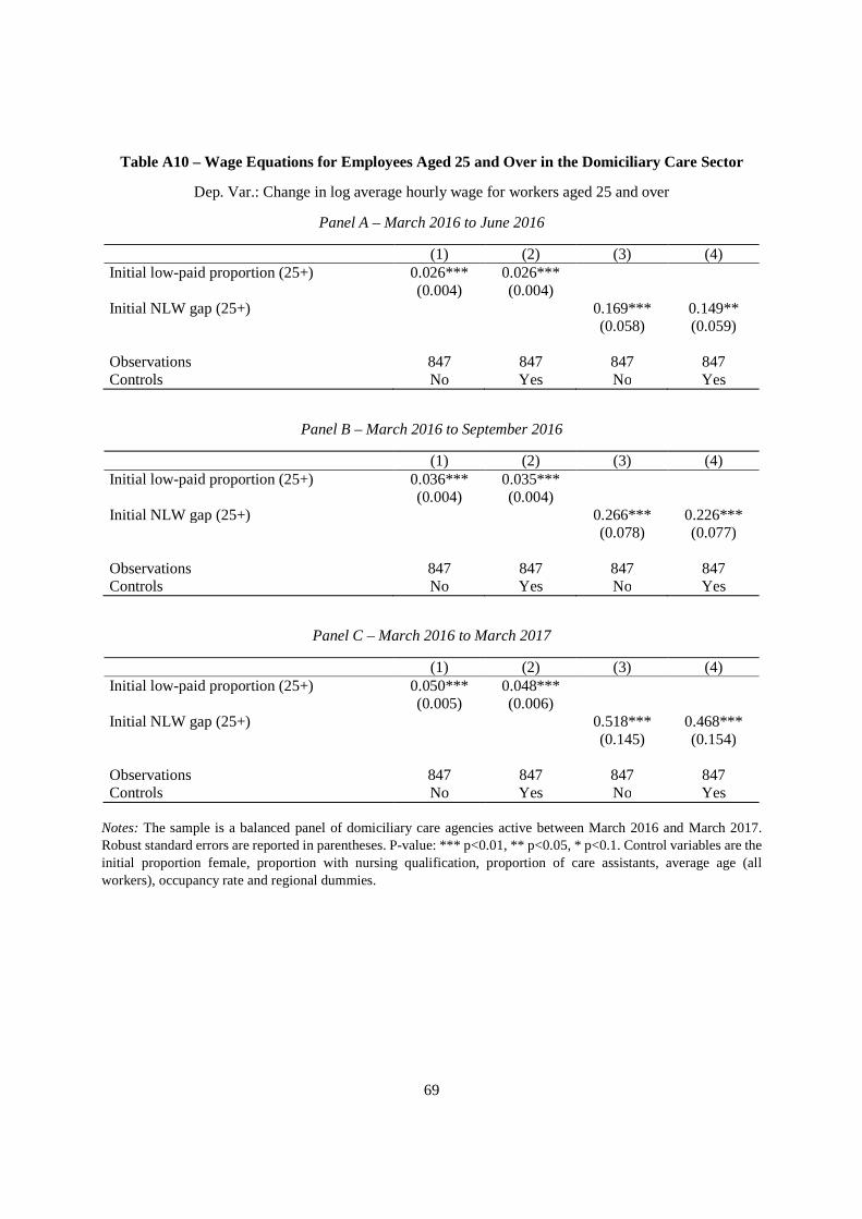
69

Table A10 – Wage Equations for Employees Aged 25 and Over in the Domiciliary Care Sector

Dep. Var.: Change in log average hourly wage for workers aged 25 and over

Panel A – March 2016 to June 2016

(1) (2) (3) (4) Initial low-paid proportion (25+) 0.026*** 0.026***

(0.004) (0.004) Initial NLW gap (25+) 0.169*** 0.149**

(0.058) (0.059)

Observations 847 847 847 847 Controls No Yes No Yes

Panel B – March 2016 to September 2016

(1) (2) (3) (4) Initial low-paid proportion (25+) 0.036*** 0.035***

(0.004) (0.004) Initial NLW gap (25+) 0.266*** 0.226***

(0.078) (0.077)

Observations 847 847 847 847 Controls No Yes No Yes

Panel C – March 2016 to March 2017

(1) (2) (3) (4) Initial low-paid proportion (25+) 0.050*** 0.048***

(0.005) (0.006) Initial NLW gap (25+) 0.518*** 0.468***

(0.145) (0.154)

Observations 847 847 847 847 Controls No Yes No Yes

Notes: The sample is a balanced panel of domiciliary care agencies active between March 2016 and March 2017. Robust standard errors are reported in parentheses. P-value: *** p<0.01, ** p<0.05, * p<0.1. Control variables are the initial proportion female, proportion with nursing qualification, proportion of care assistants, average age (all workers), occupancy rate and regional dummies.

70

Table A11 – Employment Spillover Equations in the Domiciliary Care Sector

Dep. Var.: Change in share of employees aged under 25

Panel A – March 2016 to June 2016

IV Proport. below

IV NLW gap

(1) (2) (3) (4) (5) (6) Initial low-paid proportion (25+) -0.002 -0.001

(0.003) (0.003) Initial NLW gap (25+) -0.013 -0.006

(0.036) (0.037) Change in log average wage (25+) -0.041 -0.041

(0.128) (0.241)

Observations 847 847 847 847 847 847 Controls No Yes No Yes Yes Yes

Panel B – March 2016 to September 2016

(1) (2) (3) (4) (5) (6) Initial low-paid proportion (25+) -0.003 -0.001

(0.004) (0.005) Initial NLW gap (25+) 0.006 0.025

(0.054) (0.055) Change in log average wage (25+) -0.033 0.111

(0.135) (0.260)

Observations 847 847 847 847 847 847 Controls No Yes No Yes Yes Yes

Panel C – March 2016 to March 2017

(1) (2) (3) (4) (5) (6) Initial low-paid proportion (25+) -0.006 -0.001

(0.005) (0.006) Initial NLW gap (25+) 0.005 0.055

(0.059) (0.058) Change in log average wage (25+) -0.022 0.118

(0.120) (0.129)

Observations 847 847 847 847 847 847 Controls No Yes No Yes Yes Yes

Notes: The sample is a balanced panel of domiciliary care agencies active between March 2016 and March 2017. Robust standard errors are reported in parentheses. P-value: *** p<0.01, ** p<0.05, * p<0.1. Control variables are the initial proportion female, proportion with nursing qualification, proportion of care assistants, average age (all workers), occupancy rate and regional dummies.

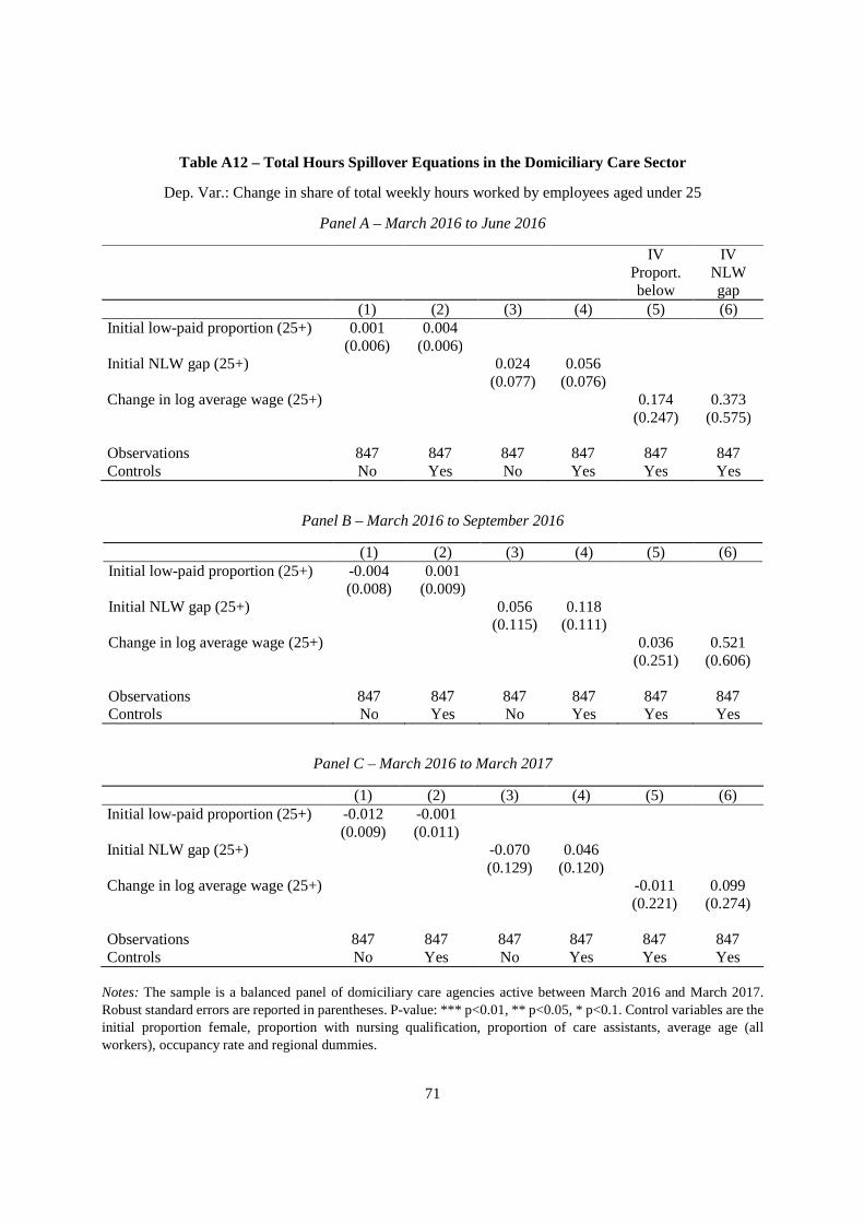
71

Table A12 – Total Hours Spillover Equations in the Domiciliary Care Sector

Dep. Var.: Change in share of total weekly hours worked by employees aged under 25

Panel A – March 2016 to June 2016

IV Proport. below

IV NLW gap

(1) (2) (3) (4) (5) (6) Initial low-paid proportion (25+) 0.001 0.004

(0.006) (0.006) Initial NLW gap (25+) 0.024 0.056

(0.077) (0.076) Change in log average wage (25+) 0.174 0.373

(0.247) (0.575)

Observations 847 847 847 847 847 847 Controls No Yes No Yes Yes Yes

Panel B – March 2016 to September 2016

(1) (2) (3) (4) (5) (6) Initial low-paid proportion (25+) -0.004 0.001

(0.008) (0.009) Initial NLW gap (25+) 0.056 0.118

(0.115) (0.111) Change in log average wage (25+) 0.036 0.521

(0.251) (0.606)

Observations 847 847 847 847 847 847 Controls No Yes No Yes Yes Yes

Panel C – March 2016 to March 2017

(1) (2) (3) (4) (5) (6) Initial low-paid proportion (25+) -0.012 -0.001

(0.009) (0.011) Initial NLW gap (25+) -0.070 0.046

(0.129) (0.120) Change in log average wage (25+) -0.011 0.099

(0.221) (0.274)

Observations 847 847 847 847 847 847 Controls No Yes No Yes Yes Yes

Notes: The sample is a balanced panel of domiciliary care agencies active between March 2016 and March 2017. Robust standard errors are reported in parentheses. P-value: *** p<0.01, ** p<0.05, * p<0.1. Control variables are the initial proportion female, proportion with nursing qualification, proportion of care assistants, average age (all workers), occupancy rate and regional dummies.

72

Table A13 – Respondent’s views about the level of NLW

All firms Balanced panel Pre-NLW Post-NLW Pre-NLW Post-NLW

(1) (2) (3) (4)

Level of NLW is About right 42.7% 52.5% 43.7% 57.4% Too low 15.0% 19.7% 16.2% 19.2% Too high 37.6% 23.7% 35.6% 20.9% Don’t know 4.7% 4.1% 4.5% 2.5% Number of respondents 1383 806 248 248

Notes: The data are from a survey of all CQC regulated English care homes that we ran before and after the NLW introduction. We obtained information on all active care homes in England from the CQC registry and sent questionnaires to all homes in January and February 2016 for the pre-NLW part of the survey, and in late June, August and November 2016 for the post-NLW part of the survey. Responses were provided by the owner manager of the care homes. We obtained a total of 1390 responses in the pre-NLW survey and of 827 responses in the post-NLW survey, of which 248 responded to both surveys. In the pre-NLW survey we asked: “Do you think that the proposed level of the NLW is: (i) about right, (ii) too high, (iii) too low, (iv) don’t know?”. In the post-NLW survey we asked: “Do you think that the current level of the NLW is: (i) about right, (ii) too high, (iii) too low, (iv) don’t know?”. The table reports respondents’ answers to these questions in the pre- and post-NLW waves for the whole sample of respondents (columns 1 and 2) and the balanced panel (columns 3 and 4).

73

Table A14 – Productivity

Dep. Var.: Change in log residents per worker hour

Panel A – March 2016 to June 2016

IV Proport. below

IV NLW gap

(1) (2) (3) (4) (5) (6) Initial low-paid proportion 0.011 0.008

(0.008) (0.009) Initial NLW gap 0.043 0.024

(0.088) (0.097) Change in log average wage 0.390 0.215

(0.435) (0.869)

Observations 4,083 4,083 4,083 4,083 4,083 4,083 Controls No Yes No Yes Yes Yes

Panel B – March 2016 to September 2016

(1) (2) (3) (4) (5) (6) Initial low-paid proportion 0.008 0.007

(0.010) (0.012) Initial NLW gap -0.010 -0.016

(0.113) (0.126) Change in log average wage 0.186 -0.064

(0.325) (0.507)

Observations 4,083 4,083 4,083 4,083 4,083 4,083 Controls No Yes No Yes Yes Yes

Notes: The sample is a balanced panel of homes active between March 2016 and March 2017. Robust standard errors are reported in parentheses. P-value: *** p<0.01, ** p<0.05, * p<0.1. Control variables are the initial proportion female, proportion with nursing qualification, proportion of care assistants, average age (all workers), occupancy rate and regional dummies.

74

Table A15 – Closures

Dep. Var.: Indicator for Firm Closure

Panel A – March 2016 to June 2016

(1) (2) (3) (4) Initial low-paid proportion 0.001 0.002

(0.002) (0.002) Initial NLW gap 0.020 0.022

(0.020) (0.024)

Observations 4,306 4,306 4,306 4,306 Controls No Yes No Yes

Panel B – March 2016 to September 2016

(1) (2) (3) (4) Initial low-paid proportion 0.001 0.003

(0.004) (0.005) Initial NLW gap 0.037 0.051

(0.037) (0.043)

Observations 4,306 4,306 4,306 4,306 Controls No Yes No Yes

Notes: The sample is a balanced panel of homes active in March 2016, unconditional on their survival until March 2017. Robust standard errors are reported in parentheses. P-value: *** p<0.01, ** p<0.05, * p<0.1. Control variables are the initial proportion female, proportion with nursing qualification, proportion of care assistants, average age (all workers), occupancy rate and regional dummies.

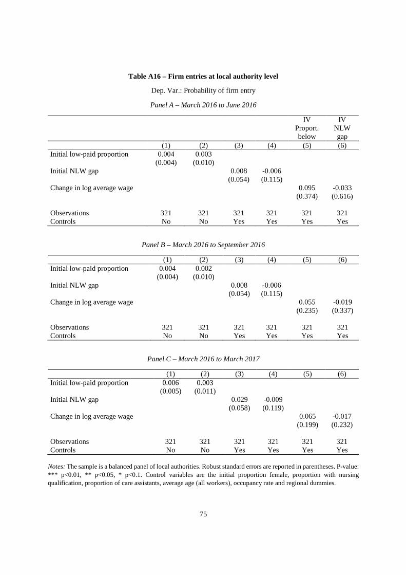
75

Table A16 – Firm entries at local authority level

Dep. Var.: Probability of firm entry

Panel A – March 2016 to June 2016

IV Proport. below

IV NLW gap

(1) (2) (3) (4) (5) (6) Initial low-paid proportion 0.004 0.003

(0.004) (0.010) Initial NLW gap 0.008 -0.006

(0.054) (0.115) Change in log average wage 0.095 -0.033

(0.374) (0.616)

Observations 321 321 321 321 321 321 Controls No No Yes Yes Yes Yes

Panel B – March 2016 to September 2016

(1) (2) (3) (4) (5) (6) Initial low-paid proportion 0.004 0.002

(0.004) (0.010) Initial NLW gap 0.008 -0.006

(0.054) (0.115) Change in log average wage 0.055 -0.019

(0.235) (0.337)

Observations 321 321 321 321 321 321 Controls No No Yes Yes Yes Yes

Panel C – March 2016 to March 2017

(1) (2) (3) (4) (5) (6) Initial low-paid proportion 0.006 0.003

(0.005) (0.011) Initial NLW gap 0.029 -0.009

(0.058) (0.119) Change in log average wage 0.065 -0.017

(0.199) (0.232)

Observations 321 321 321 321 321 321 Controls No No Yes Yes Yes Yes

Notes: The sample is a balanced panel of local authorities. Robust standard errors are reported in parentheses. P-value: *** p<0.01, ** p<0.05, * p<0.1. Control variables are the initial proportion female, proportion with nursing qualification, proportion of care assistants, average age (all workers), occupancy rate and regional dummies.

76

Table A17 – Firm exits at local authority level

Dep. Var.: Probability of firm exit

Panel A – March 2016 to June 2016

IV Proport. below

IV NLW gap

(1) (2) (3) (4) (5) (6) Initial low-paid proportion 0.004 0.006

(0.003) (0.004) Initial NLW gap 0.029 0.055

(0.022) (0.037) Change in log average wage 0.225 0.294

(0.153) (0.224)

Observations 321 321 321 321 321 321 Controls No No Yes Yes Yes Yes

Panel B – March 2016 to September 2016

(1) (2) (3) (4) (5) (6) Initial low-paid proportion 0.001 -0.004

(0.007) (0.009) Initial NLW gap 0.002 -0.008

(0.061) (0.078) Change in log average wage -0.106 -0.023

(0.220) (0.229)

Observations 321 321 321 321 321 321 Controls No No Yes Yes Yes Yes

Panel C – March 2016 to March 2017

(1) (2) (3) (4) (5) (6) Initial low-paid proportion 0.003 0.004

(0.014) (0.018) Initial NLW gap -0.030 -0.036

(0.123) (0.162) Change in log average wage 0.073 -0.070

(0.338) (0.319)

Observations 321 321 321 321 321 321 Controls No No Yes Yes Yes Yes

Notes: The sample is a balanced panel of local authorities. Robust standard errors are reported in parentheses. P-value: *** p<0.01, ** p<0.05, * p<0.1. Control variables are the initial proportion female, proportion with nursing qualification, proportion of care assistants, average age (all workers), occupancy rate and regional dummies.

CENTRE FOR ECONOMIC PERFORMANCE Recent Discussion Papers

1532 Swati Dhingra Rebecca Freeman Eleonora Mavroeidi

Beyond Tariff Reductions: What Extra Boost From Trade Agreement Provisions?

1531 Doruk Cengiz Arindrajit Dube Attila Lindner Ben Zipperer

The Effect of Minimum Wages on Low-Wage Jobs: Evidence from the United States Using a Bunching Estimator

1530 Stephen Gibbons Vincenzo Scrutinio Shqiponja Telhaj

Teacher Turnover: Does it Matter for Pupil Achievement?

1529 Ghazala Azmat Stefania Simion

Higher Education Funding Reforms: A Comprehensive Analysis of Educational and Labour Market Outcomes in England

1528 Renata Lemos Daniela Scur

All in the Family? CEO Choice and Firm Organization

1527 Stephen Machin Matteo Sandi

Autonomous Schools and Strategic Pupil Exclusion

1526 Stephan E. Maurer Oil Discoveries and Education Spending in the Postbellum South

1525 Paola Conconi Manuel García-Santana Laura Puccio Roberto Venturini

From Final Goods to Inputs: The Protectionist Effect of Rules of Origin

1524 Zack Cooper Fiona Scott Morton Nathan Shekita

Surprise! Out-of-Network Billing for Emergency Care in the United States

1523 Zack Cooper Amanda Kowalski Eleanor Neff Powell Jennifer Wu

Politics, Hospital Behaviour and Health Care Spending

1522 Philippe Aghion Ufuk Akcigit Ari Hyytinen Otto Toivanen

The Social Origins of Inventors

1521 Andrés Barrios F. Giulia Bovini

It’s Time to Learn: Understanding the Differences in Returns to Instruction Time

1520 Sara Calligaris Massimo Del Gatto Fadi Hassan Gianmarco I.P. Ottaviano Fabiano Schivardi

The Productivity Puzzle and Misallocation: An Italian Perspective

1519 Alex Bell Raj Chetty Xavier Jaravel Neviana Petkova John Van Reenen

Who Becomes an Inventor in America? The Importance of Exposure to Innovation

1518 Randolph Bruno Nauro Campos Saul Estrin Meng Tian

Economic Integration, Foreign Investment and International Trade: The Effects of Membership of the European Union

1517 Fabrice Defever José-Daniel Reyes Alejandro Riaño Miguel Eduardo Sánchez-Martín

Special Economic Zones and WTO Compliance: Evidence from the Dominican Republic

1516 Philippe Aghion Ufuk Akcigit Matthieu Lequien Stefanie Stantcheva

Tax Simplicity and Heterogeneous Learning

The Centre for Economic Performance Publications Unit Tel: +44 (0)20 7955 7673 Email info@cep.lse.ac.uk Website: http://cep.lse.ac.uk Twitter: @CEP_LSE