ISSN 2042-2695

CEP Discussion Paper No 1221

May 2013

A Question of Degree:

The Effects of Degree Class on Labor Market Outcomes

Andy Feng and Georg Graetz

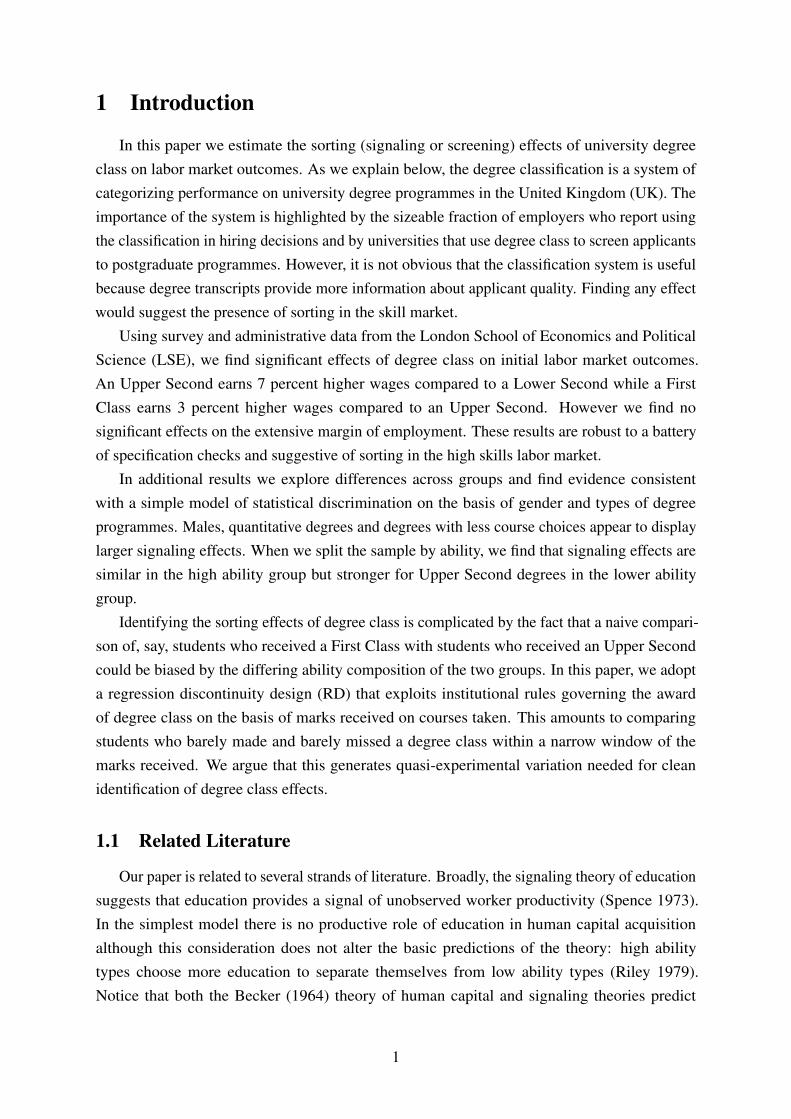
Abstract In this paper we estimate the sorting effects of university degree class on initial labor market

outcomes using a regression discontinuity design that exploits institutional rules governing

the award of degrees. Consistent with anecdotal evidence, we find sizeable and significant

effects for Upper Second degrees and positive but smaller effects for First Class degrees on

wages. In additional results we explore differences across groups and find evidence

consistent with a simple model of statistical discrimination on the basis of gender and types

of degree programmes. When we split the sample by ability, we find that the signaling effects

are similar in the high ability group but stronger for Upper Second degrees in the lower

ability group. The evidence points to the importance of sorting in the high skills labor market.

Keywords: degree classification, regression discontinuity design, sorting effects

JEL Classifications: I24, J24, J31

This paper was produced as part of the Centre’s Productivity and Innovation Programme. The

Centre for Economic Performance is financed by the Economic and Social Research Council.

Acknowledgements We would like to thank Lucy Burrows from LSE Careers and Tom Richey from Student

Records for their kind assistance with the data. We thank participants at the LSE labour

economics workshop for helpful comments. Any remaining errors are our own. The views

and opinions expressed herein are those of the authors and do not necessarily reflect the

views of LSE.

Andy Feng and Georg Graetz are PhD students and researchers at the Centre for

Economic Performance, London School of Economics and Political Science.

Published by

Centre for Economic Performance

London School of Economics and Political Science

Houghton Street

London WC2A 2AE

All rights reserved. No part of this publication may be reproduced, stored in a retrieval

system or transmitted in any form or by any means without the prior permission in writing of

the publisher nor be issued to the public or circulated in any form other than that in which it

is published.

Requests for permission to reproduce any article or part of the Working Paper should be sent

to the editor at the above address.

A. Feng and G. Graetz, submitted 2013

1 Introduction

In this paper we estimate the sorting (signaling or screening) effects of university degreeclass on labor market outcomes. As we explain below, the degree classification is a system ofcategorizing performance on university degree programmes in the United Kingdom (UK). Theimportance of the system is highlighted by the sizeable fraction of employers who report usingthe classification in hiring decisions and by universities that use degree class to screen applicantsto postgraduate programmes. However, it is not obvious that the classification system is usefulbecause degree transcripts provide more information about applicant quality. Finding any effectwould suggest the presence of sorting in the skill market.

Using survey and administrative data from the London School of Economics and PoliticalScience (LSE), we find significant effects of degree class on initial labor market outcomes.An Upper Second earns 7 percent higher wages compared to a Lower Second while a FirstClass earns 3 percent higher wages compared to an Upper Second. However we find nosignificant effects on the extensive margin of employment. These results are robust to a batteryof specification checks and suggestive of sorting in the high skills labor market.

In additional results we explore differences across groups and find evidence consistentwith a simple model of statistical discrimination on the basis of gender and types of degreeprogrammes. Males, quantitative degrees and degrees with less course choices appear to displaylarger signaling effects. When we split the sample by ability, we find that signaling effects aresimilar in the high ability group but stronger for Upper Second degrees in the lower abilitygroup.

Identifying the sorting effects of degree class is complicated by the fact that a naive compari-son of, say, students who received a First Class with students who received an Upper Secondcould be biased by the differing ability composition of the two groups. In this paper, we adopta regression discontinuity design (RD) that exploits institutional rules governing the awardof degree class on the basis of marks received on courses taken. This amounts to comparingstudents who barely made and barely missed a degree class within a narrow window of themarks received. We argue that this generates quasi-experimental variation needed for cleanidentification of degree class effects.

1.1 Related Literature

Our paper is related to several strands of literature. Broadly, the signaling theory of educationsuggests that education provides a signal of unobserved worker productivity (Spence 1973).In the simplest model there is no productive role of education in human capital acquisitionalthough this consideration does not alter the basic predictions of the theory: high abilitytypes choose more education to separate themselves from low ability types (Riley 1979).Notice that both the Becker (1964) theory of human capital and signaling theories predict

1

a positive correlation between ability and education. Thus discriminating between the twotheories has proven challenging empirically (Weiss 1995). Complementing the signaling theoriesare screening models where employers take actions to separate workers into ability groups(Stiglitz 1975, Wolpin 1977). We follow Weiss (1995) in collectively describing these classes ofsignaling and screening theories as sorting models.

Empirical testing of sorting models has proceeded in two ways. Indirect evidence comes inthe form of changes in the human capital investment decisions of one ability group from changesin the decisions made in other groups. Compulsory schooling laws for primary education thataffect higher education groups (Lang and Kropp 1986) or tertiary enrolment changes that affectthe high school margin (Bedard 2001) are seen as consistent with the signaling value of educationbut not human capital theories. More direct evidence imagines a randomized experiment whererandomly selected individuals from the same ability group get treated with an educational signal.Tyler, Murnane, and Willet (2002) mimic this experiment by exploiting differences in passingstandards for the GED diploma across US states. Their finding of significant effects for whitemales stands in contrast to Clark and Martorell (2010) who find no effects for receiving the highschool diploma.

For tertiary education the early literature looked at the credential effects associated thecompletion of college degrees (Layard and Psacharopoulos 1974). Hungerford and Solon(1987), Belman and Heywood (1991) and Jaeger and Page (1996) include dummy variables forcollege completion in Mincer (1974) regressions and interpret the significant effects of collegecompletion as signals of underlying correlates of productivity. In papers most closely relatedto ours, Di Pietro (2010), Ireland, Naylor, Smith, and Telhaj (2009) and McKnight, Naylor,and Smith (2007) examine the signaling effects of degree classification for students in the UK.Notably Di Pietro (2010) adopts a regression discontinuity design using final year marks andfinds no effect on employment. We get similar results and extend the analysis by looking atwage differences. Ireland, Naylor, Smith, and Telhaj (2009) use OLS regressions and find 4 and5 percent returns to First Class and Upper Second degrees respectively. Their sample consists ofa much larger dataset of UK students across many universities and years but does not have thecourse history information we have to construct finer comparison groups.

The rest of the paper is organized as follows. In Section 2 we discuss the institutional setting,in Section 3 we explore the data sources and empirical strategy, in Section 4 we present ourresults and specification checks. Section 5 explores heterogeneity across programmes and abilitygroups. Finally, in Section 6 we conclude.

2

2 Institutional Setting

2.1 University Description

Our data comes from the London School of Economics and Political Science (LSE). LSEis a top ranked public research university located in London, UK, specializing in the socialsciences. LSE offers a range of degree programmes and admission is highly competitive. In2012, LSE students came top for employability in the Sunday Times University Guide with overthree quarters of students in employment or further studies six months after graduating. Ourresults thus speak to the high end of the skills market within a selective tertiary institution.1

2.2 UK Degree Classification

The degree classification system in the UK is a grading scheme for degrees. The highestdistinction for an undergraduate is the First Class honors followed by the Upper Second, LowerSecond, Third Class and Pass degrees. While all universities in the UK follow this classificationscheme, each university has the power and discretion to apply its own standards and rules todetermine the distribution of degrees. The system has been applied in other countries includingAustralia, Canada, India and many Commonwealth nations. In the US, a system of gradepoint averages (GPA) and Latin Honors performs the similar purpose of classifying degrees. Inprinciple, this implies that our results apply to a broad range of countries.2 Anecdotal evidencepoints to the increasing importance of degree class in hiring decisions. One report points to75 percent of employers in 2012 requiring at least an Upper Second degree as minimum entryrequirement especially for competitive jobs–this compares to 52 percent in 2004.3

2.3 LSE Degree Classification Rules

To construct our identification strategy, we exploit a unique feature of the rules governingthe award of degree class. Undergraduates in the LSE take nine courses over three years. Everycourse is graded out of 100 marks and fixed thresholds are used to map the marks to degreeclass. As shown in Table B.1, a First Class Honors degree requires 5 marks of 70 or above or 4marks of 70 or above with aggregate marks of at least 590. This mapping from course marks tofinal degree class applies to all departments and years.4

1See LSE website http://www2.lse.ac.uk/intranet/CareersAndVacancies/graduateDestinations/6monthson.aspx.

2See wikipedia http://en.wikipedia.org/wiki/British_undergraduate_degree_classification and http://en.wikipedia.org/wiki/Latin_honors. The GPA is usually ascale from 0 to 4 with one decimal accuracy and is a finer measure of performance than the UK system. There havebeen calls to scrap the UK system in favor of a US-style points system, the Guardian, July 9th 2012.

3See the Daily Telegraph, July 4th 2012 and the Guardian, July 4th 2012.4Four courses are taken each year, however only the average of the best three courses in the first year

counts towards final classification. Undergraduate law students are an exception and follow a different set ofrules. We exclude them from all analyses. Full details of the classification system is available online at http:

3

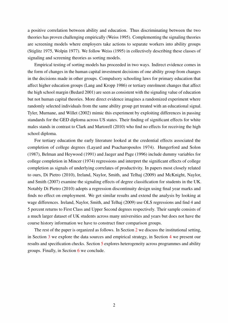
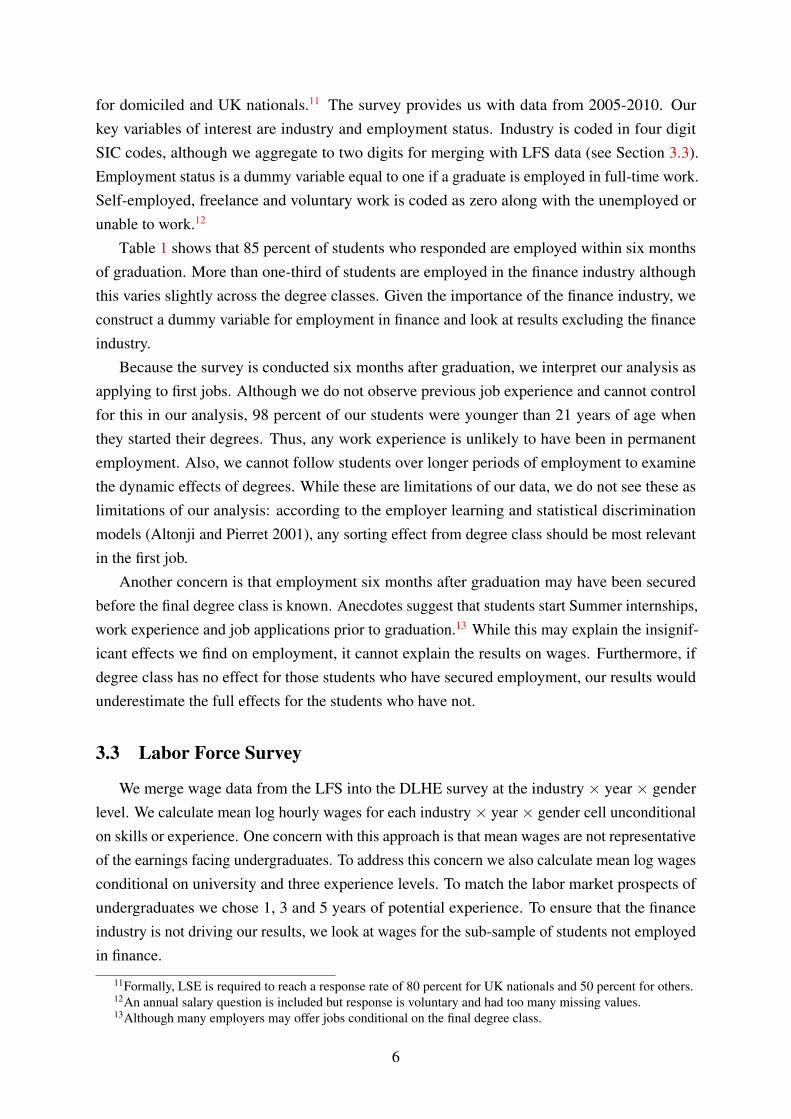
We exploit the discontinuous relationship between degree class and marks received on thefourth highest mark in a regression discontinuity design (RD). Our strategy is intuitive andamounts to comparing otherwise similar students who differ only in a critical course mark whichdetermines their final degree class. To be specific, let us consider the award of a First Classdegree which depends on the receipt of at least four first class marks. This suggests that thefourth highest mark for any student plays a critical role in determining the degree class. Astudent whose fourth highest mark is larger than 70 is much more likely to obtain a First Classdegree than a student whose mark just missed 70, everything else equal. This can be seen clearlyin Figure 1 which plots the fraction of students who receive a First Class degree against theirfourth highest mark received. There is a clear jump in the probability of receiving a First Classafter the 70-mark threshold. A similar story can be seen in the award of an Upper Second degreeat the 60-mark threshold. To summarize, the fourth highest mark plays the role of the assignmentvariable in our RD strategy.

In reality, we employ a fuzzy RD design because there are complications to the rules. Asshown in Table B.1 there is an aggregate mark requirement. Additionally, a failed courseresults in a downgrade in degree class.5 These caveats do not threaten our research designbecause they are not applied on a case-by-case basis but are applied impartially at the departmentlevel.6 Nevertheless it moves us away from a sharp RD design. We explore in detail the first-stage relationship between degree class and fourth highest mark in Section 4.1 and show thatthe relevant complier population is sizeable so that our results generalize to the larger LSEpopulation.

3 Data and Empirical Strategy

3.1 Students’ Demographics and Course History

From student records we obtain age, gender, nationality and country of domicile information.Course history includes information on degree programme, courses taken and grades awarded,and eventual degree classification. Table 1 reports the descriptive statistics of the variables usedin our analysis. We have 5,912 students in the population from 2005-2010 of which 2,649 areincluded in the DLHE survey (described in detail below). Columns (1) and (4) report the meanand standard deviations of variables for surveyed and non-surveyed students, respectively, whilecolumn (5) reports the difference. Surveyed students are less likely to be female, more likelyto be UK nationals, more likely to receive an Upper Second and less likely to receive a Lower

//www.lse.ac.uk/resources/calendar/academicRegulations/BA-BScDegrees.htm.5Failed courses can be retaken up to three times and the better grade is used in calculating final degree class.

We control for any failed or retaken courses in our estimation. Students can appeal on specific courses, but thisdoes not worry us. First, appeals are difficult and rarely successful. Second, a student does not usually know beforethe completion of their degree which course is critical in determining their class.

6There could still be a concern if departments can upgrade students who appeal in their final degree classification.But this would not retroactively change grades on courses taken and reinforces the need to use a fuzzy RD design.

4

Second.To implement our empirical strategy, we further split the surveyed students into two samples.

The First Class sample consists of students who received either a First Class or an Upper Secondand the Upper Second sample consists of students who received either an Upper Second orLower Second. This provides two discontinuities that we examine separately and narrowsour comparisons to students who are on either side of each threshold. In Table 1 First Class,Upper Second and Lower Second are dummy variables for the degree classes. Among allsurveyed students, the majority of 60 percent received an Upper Second with the remaining 40percent roughly evenly split between First Class and Lower Second. 1[4th MARK ≥ 70] and1[4th MARK ≥ 60] are dummy variables equal to one if the fourth highest mark is no less than70 or 60 respectively.7

One shortcoming of this database is that we do not have measures of a student’s pre-universityability. For a typical UK student this might include his GCSE and A-level results. Althoughadmissions to LSE programmes require A-level or equivalent results, this data is not collectedcentrally but is administered at the department level. While controlling for ability is unnecessaryin our identification strategy it would be useful for improving precision and interesting to checkour results against different ability groups.8 We take some steps to redress this shortcoming.First in all our regressions we control for department × year interactions. More directly we usethe admissions offers made at the programme level as a measure of student ability. In Table B.3we classify degree programmes into groups based on A-level requirements. The most stringentprogrammes require A*AA grades followed by AAA, AAB and ABB respectively. We also codea dummy variable indicating A-level mathematics’ requirements for admissions.9 Section 5presents results exploring heterogeneity over these programme attributes.

3.2 Destination of Leavers from Higher Education Survey

The DLHE survey is a national survey of students who have recently graduated from auniversity in the UK. This survey is conducted twice a year to find out employment circumstancesof students six months after graduation.10 Due to the frequency of the survey and its statutorynature, LSE oversees the survey and reports the results to HESA (Higher Education StatisticsAuthority). The survey is sent by email and responded to online and in theory includes allstudents including non-domiciled and non-UK nationals. In practice response rates are higher

7We split the sample because anecdotes suggest that the Upper Second threshold may be more important. Italso allows a cleaner non-parametric identification strategy around the two discontinuities. We dropped Third Classand below because they constituted less than 5 percent of the population. Including them among the Lower Secondpopulation does not change results.

8As noted in Lee and Lemieux (2010) an RD design mimics a natural experiment close to the discontinuity.Hence there should be no need for additional controls except to improve precision of estimates.

9Results in (McKnight, Naylor, and Smith 2007) suggest that controlling for degree programme reduces theimportance of pre-university academic results.

10The surveys are conducted from November to March for the “January” survey, and from April to June for the“April” survey.

5

for domiciled and UK nationals.11 The survey provides us with data from 2005-2010. Ourkey variables of interest are industry and employment status. Industry is coded in four digitSIC codes, although we aggregate to two digits for merging with LFS data (see Section 3.3).Employment status is a dummy variable equal to one if a graduate is employed in full-time work.Self-employed, freelance and voluntary work is coded as zero along with the unemployed orunable to work.12

Table 1 shows that 85 percent of students who responded are employed within six monthsof graduation. More than one-third of students are employed in the finance industry althoughthis varies slightly across the degree classes. Given the importance of the finance industry, weconstruct a dummy variable for employment in finance and look at results excluding the financeindustry.

Because the survey is conducted six months after graduation, we interpret our analysis asapplying to first jobs. Although we do not observe previous job experience and cannot controlfor this in our analysis, 98 percent of our students were younger than 21 years of age whenthey started their degrees. Thus, any work experience is unlikely to have been in permanentemployment. Also, we cannot follow students over longer periods of employment to examinethe dynamic effects of degrees. While these are limitations of our data, we do not see these aslimitations of our analysis: according to the employer learning and statistical discriminationmodels (Altonji and Pierret 2001), any sorting effect from degree class should be most relevantin the first job.

Another concern is that employment six months after graduation may have been securedbefore the final degree class is known. Anecdotes suggest that students start Summer internships,work experience and job applications prior to graduation.13 While this may explain the insignif-icant effects we find on employment, it cannot explain the results on wages. Furthermore, ifdegree class has no effect for those students who have secured employment, our results wouldunderestimate the full effects for the students who have not.

3.3 Labor Force Survey

We merge wage data from the LFS into the DLHE survey at the industry × year × genderlevel. We calculate mean log hourly wages for each industry × year × gender cell unconditionalon skills or experience. One concern with this approach is that mean wages are not representativeof the earnings facing undergraduates. To address this concern we also calculate mean log wagesconditional on university and three experience levels. To match the labor market prospects ofundergraduates we chose 1, 3 and 5 years of potential experience. To ensure that the financeindustry is not driving our results, we look at wages for the sub-sample of students not employedin finance.

11Formally, LSE is required to reach a response rate of 80 percent for UK nationals and 50 percent for others.12An annual salary question is included but response is voluntary and had too many missing values.13Although many employers may offer jobs conditional on the final degree class.

6

This gives us five different measures of industry wages–overall mean, university with 1, 3and 5 years of experience and overall mean for non-finance industries. Our preferred measure isthe overall mean because it provides a clean measure of the industry’s “rank” compared to otherindustries. In any case the five measures are highly correlated with pairwise correlations neverless than 0.8. Table 1 shows that the mean log wage is 2.45 which is roughly £11.60 per hour in2005£. As expected, industry wages increase in years of experience.

Using industry wages implies that we do not have within-industry variation in outcomes. Tothe extent that within-industry comparisons matter, our results will not be representative of thetrue effects of degrees. We acknowledge that this is an imperfect measure and are cautious ininterpreting our results as effects on industry not individual wages.14 Table B.2 shows the top 15industries ranked by total share of employment. Even accounting for the large share in finance,there is substantial distribution in employment across industries–of the 84 two-digit SIC codes,66 are represented in our data.

3.4 Empirical Strategy

Our unit of observation is a student. For each student we observe his degree classificationand his course grades. In particular, we observe his fourth highest mark out of nine coursestaken over three years of the degree. As described in Section 2.3, institutional rules imply thatthe fourth highest mark is critical in determining his degree class. When the fourth highestmark crosses the 70-mark or 60-mark cutoff, there is a discontinuous jump in the probability ofreceiving a First Class and Upper Second respectively. In Section 4.4 we show that includingthe other marks as controls does not change our results.

Identification in an RD setup requires two assumptions (Lee and Lemieux 2010). First,agents cannot precisely manipulate the assignment variable. Second, apart from the treatment–inthis case degree class–all other observables and unobservables vary continuously across thethreshold. The first assumption cannot directly be tested although institutional knowledge andthe McCrary test provide supporting evidence. These are discussed in Section 4.2. The secondassumption can be tested using data on observables once the assignment variable has beencontrolled for flexibly. Flexible control of the assignment variable can be done in several ways.A parametric function such as a high order polynomial is parsimonious but is found to be quitesensitive to polynomial order (Angrist and Pischke 2009). A non-parametric approach observesthat a regression discontinuity can be thought of as a kernel regression at a boundary point(Imbens and Lemieux 2008). This motivates the use of local regressions with various kernelsand bandwidths (Fan and Gijbels 1996, Li and Racine 2007).15

In our benchmark specification we use the simplest non-parametric local linear regression

14The lack of a more direct wage measure is an issue for other studies in the literature as well (Di Pietro 2010,McKnight, Naylor, and Smith 2007).

15Regression discontinuity was introduced by Thistlethwaite and Campbell (1960) and formalized in thelanguage of treatment effects by Hahn, Todd, and van der Klaauw (2001).

7

with a rectangular bandwidth of 5 marks above and below the cutoff (Imbens and Wooldridge2009). This means we include the fourth mark linearly and interacted with the dummy variable asadditional controls. In specification checks we vary the bandwidth and try polynomial functionsto flexibly control for the fourth mark. As discussed in Section 4.4 these specification checksproduce consistent results. The non-deterministic relationship between fourth highest mark anddegree class means that in practice we employ a fuzzy RD design. This uses the fourth highestmark as an instrument for degree class.16

In theory, identification in an RD setup comes in the limit as we approach the discontinuityasymptotically (Hahn, Todd, and van der Klaauw 2001). In practice, this requires sufficientdata around the boundary points–as we get closer to the discontinuity estimates tend to get lessprecise because we have fewer data. Furthermore, when the assignment variable is discreteby construction, there is the additional complication that we cannot approach the boundaryinfinitesimally.17 In this paper, we choose the 5 mark bandwidth as a reasonable starting pointand accept that some of the identification necessarily comes from marks away from the boundary.We follow Lee and Card (2008) in correcting standard errors for the discrete structure of ourassignment variable by clustering on marks throughout.

We can write the first-stage equation as:

CLASSi(1)

=δ0 + δ11[4th MARK ≥ cutoff]i + δ2(4th MARKi − cutoff)+

δ3(4th MARKi − cutoff)× 1[4th MARK ≥ cutoff]i +Xiδ4 + ui

where CLASS is either First Class or Upper Second and the cutoff is 70 or 60 respectively.1[4th MARK ≥ cutoff] is a dummy variable for the fourth mark crossing the cutoff and ourinstrument for the potentially endogenous degree class. X is a vector of covariates includingfemale dummies, age and age squared, dummies for being a UK national, dummies for havingresat or failed any course, 15 dummies for department, 5 year dummies and 75 dummies fordepartment × year interactions.

We can use the predicted degree class from our first-stage regression in our second-stageequation:

Yi =β0 + β1CLASSi + β2(4th MARKi − cutoff)+(2)

β3(4th MARKi − cutoff)× 1[4th MARK ≥ cutoff]i +Xiβ4 + εi

where Y are various labor market outcomes including employment status, employment in finance

16The close connection between fuzzy RD and instrumental variables is noted in Lee and Lemieux (2010),Imbens and Lemieux (2008) and Imbens and Wooldridge (2009). Instead of the usual exclusion restrictions,however, we require the continuity assumption and non-manipulation of the assignment variable.

17This is also a problem facing designs where age in years or months is the assignment variable, e.g. Carpenterand Dobkin (2009).

8

industry and five measures of industry wages.

4 Results

4.1 First-Stage and Reduced Form Regressions

In this section we look at estimates of the first-stage Equation (1) and the reduced formregressions:

Yi =γ0 + γ11[4th MARK ≥ cutoff]i + γ2(4th MARKi − cutoff)+(3)

γ3(4th MARKi − cutoff)× 1[4th MARK ≥ cutoff]i +Xiγ4 + νi

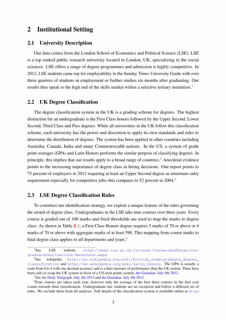
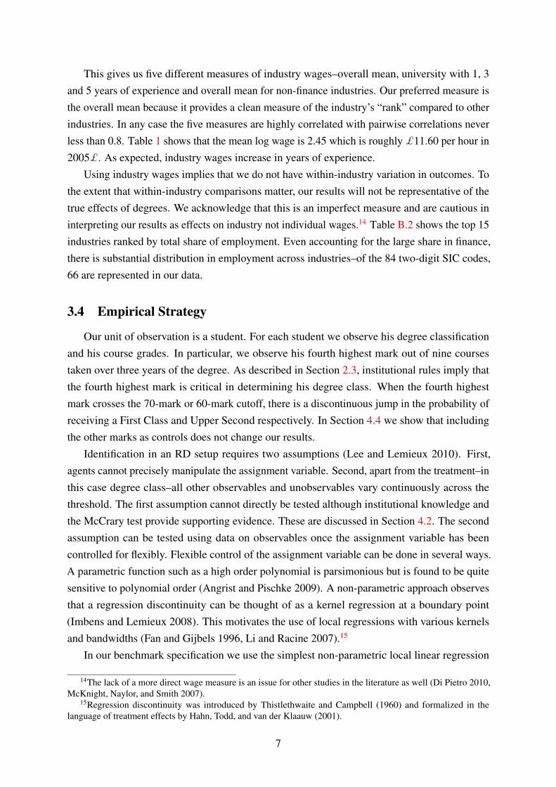
where Y are the various labor market outcomes. Table 2, column (1) reports the first-stageresults for the First Class discontinuity (panel A) and Upper Second discontinuity (panel B).Both first-stage F-statistics are above the rule-of-thumb threshold of 10 and mitigates anyconcerns about weak instruments (Stock, Wright, and Yogo 2002).18 In order to better interpretthe first-stage, we can look at the relationship between fourth highest mark and degree classwithout controlling for any covariates. This also allows us to do a simple count of the complierpopulation in LSE (Angrist, Imbens, and Rubin 1996, Imbens and Angrist 1994). In Figure 2the schematic shows the breakdown of students into compliers, always takers and never takersaround the discontinuity. For instance, always takers are students who receive a First Classregardless of their fourth highest mark, while compliers are students who receiver a First Classbecause their fourth highest mark crosses the threshold. The breakdown suggests that thecomplier population is sizeable at 87 percent. This is expected because the institutional rules arestrictly followed and supports the validity of our results to the rest of the LSE population.

Columns (2) to (8) regress the outcome variables on the excluded instrument always control-ling for covariates. In panel A, the small magnitudes and insignificant results suggest that theFirst Class may not be important in labor market outcomes. The larger and significant results forUpper Second in panel B are consistent with the idea that an Upper Second is important as asignal or screening device for employers.

4.2 Randomization Checks and McCrary Test

As discussed in Section 3.4, identification in an RD setup requires continuity in the observ-ables (and unobservables) across the threshold as well as non-manipulation of the assignmentvariable. To test for continuity in the observables, we regress each covariate on the treatmentdummy in Table 3, columns (1) to (5). Apart from age in the First Class sample and genderin the Upper Second sample, the results are consistent with the lack of discontinuity in the

18The sample size varies over outcome variables but we confirmed that the first-stage and other results are notsensitive to these sample differences.

9

observables. The apparent discontinuity in age and gender does not worry us because these arenon-manipulable attributes (Holland 1986). In other words, there is less concern that agentscould have taken actions to manipulate these attributes around the discontinuity to improve theirdegree class. This would be the case if we saw discontinuities in the students who resat or failedany courses.

To test for the manipulation of the assignment variable itself, McCrary (2008) suggests usingthe frequency count as the dependent variable in the RD setup. The idea is that manipulation ofthe assignment variable should result in bunching of individuals at the cutoff. In the educationliterature, this was shown to be an important invalidation of the RD approach (see for e.g.Urquiola and Verhoogen (2009)). In our case, we should see a jump in the number of studentsat the threshold of 70 or 60 marks. In column (6) of Table 3 we perform the McCrary test andfind large and (in the case of the Upper Second threshold) significant jumps in the number ofstudents. Prima facie this might suggest that students are manipulating their marks in order toreceive better degrees.

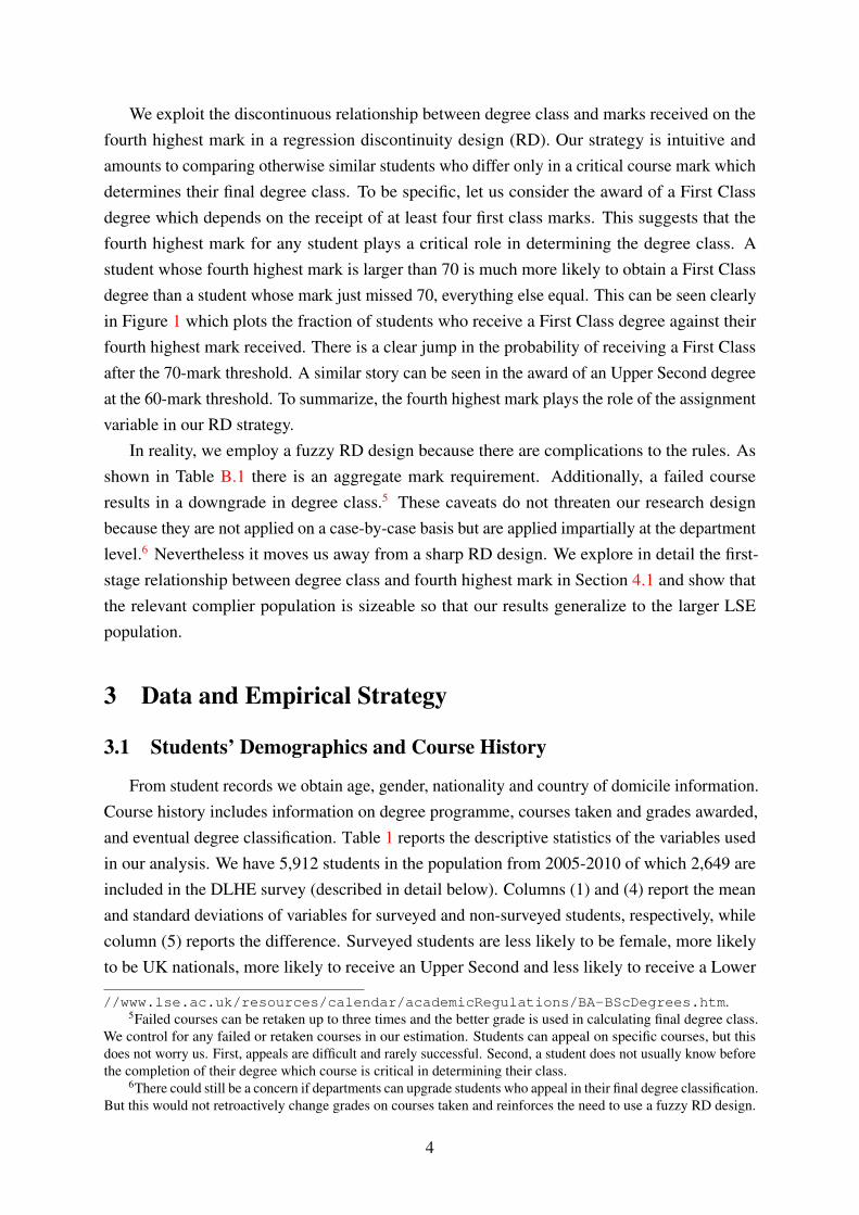
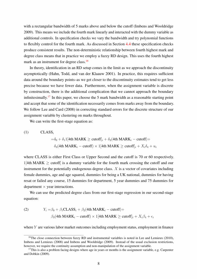
We argue that this bunching is not the result of manipulation but is a consequence ofinstitutional features. Figure 3 plots the histogram of the fourth, fifth and highest marks. Inevery case there is a clear bunching of marks at 60 and 70 even for the highest mark whichis not critical for eventual degree class. This is because exam graders actively avoid givingborderline marks (i.e. 59 or 69) and either round up or down.19 One may still worry that studentswho received 58 or 68 may appeal to have their script re-graded. From discussions with staff,the appeals process is arduous and rarely successful. Nonetheless we follow the literature indealing with the potential manipulation of marks by excluding the threshold in specificationchecks reported in Section 4.4 (see for e.g. Almond and Doyle (2011)). This does not changeour results.

4.3 Effects of Degree Class on Labor Market Outcomes

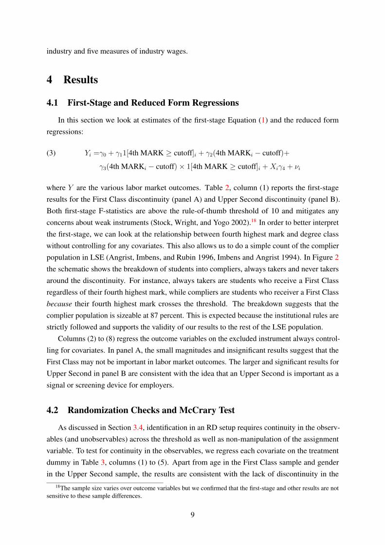
Table 4 reports the results for the effects of receiving a First Class degree compared with anUpper Second. In panel A, we compare average differences in outcomes without controlling forany covariates. There are no differences in employment in general or in the finance industryspecifically. However, there are significant differences in industry wages. Using our preferredmeasure of mean industry log wages, a First Class receives 7 percent higher wages. Panel Bincludes covariates to allow for closer comparisons of students. This corresponds to Equation (2).The employment outcomes remain insignificant while the wage coefficients halve but remainsignificant. Finally in panel C, we instrument for First Class using a dummy variable for thefourth highest mark, as in Equation (1). Although the difference in industry mean wages remainssignificant at 5 percent, the conditional experience measures are insignificant suggesting that the

19In LSE, exams are taken anonymously and each script is graded by one internal and one external examiner.Having graded each script separately, graders convene to deliberate on the final mark.

10

wage differences for a First Class are not sizeable.Table 5 reports the same specifications as Table 4 but for the Upper Second degree. Sur-

prisingly, there are no differences in average outcomes across students without controlling forcovariates in panel A. This is because of inter-departmental comparisons we are making inthe absence of department fixed effects. Once we control for covariates including departmentby year fixed effects in panel B we observe that an Upper Second receives 4 percent higherwages than a Lower Second. An Upper Second also has a 7 percentage point (20 percent) higherprobability of working in finance. Using the threshold dummy variable 1[4th MARK ≥ 60] asan instrument for Upper Second, panel C reveals that the returns are significant and sizeable at 7percent for mean wages and 12 percentage points (37 percent) for finance industry employment.

To interpret these results we translate the percentage differences to pounds. Using ourpreferred measure of wages in the specification in column (3) we find that a First Class andUpper Second are worth around £1,000 and £2,040 per annum respectively in current money.20

4.4 Specification Checks

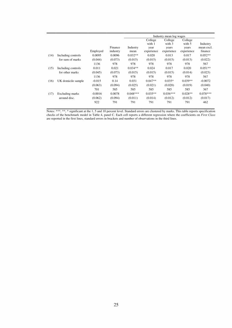
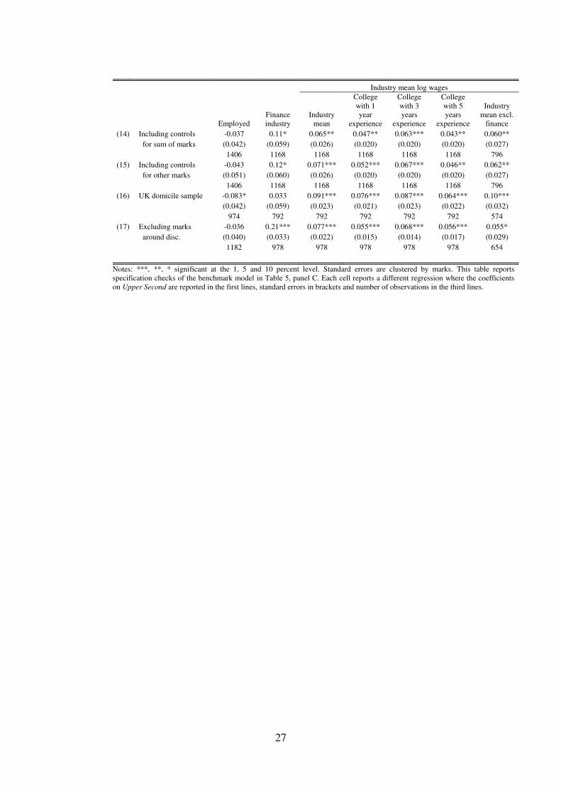
Here we conduct a battery of specification tests for our benchmark models given in panelsC of Table 4 and Table 5. In Table 6 we report checks for the First Class degree while Table 7reports the same for Upper Second. Row (1) reports the benchmark results for convenience.Rows (2) to (10) report results using different bandwidth sizes (our benchmark is a 5-markbandwidth) and rows (11) to (14) report specifications using parametric polynomial controls. Inrows (14) and (15) we include controls for the sum of marks and other marks separately to showthat our results are not driven by omission of other course grades. In row (16) we address theconcern that our results misrepresent students who are not domiciled in UK by looking onlyat domiciled students. In row (17) we deal with the worry that bunching of marks around thethreshold reflects manipulation.

Employment outcomes appear to be sensitive to bandwidth choice. For the First Class somespecifications even suggest a negative effect on employment, e.g. rows (3) and (4). Likewisefor the Upper Second degree, employment overall and in finance does not display a consistentpattern across specifications. To be conservative we interpret this as suggesting that the extensivemargin is not affected by degree class. This may be due to the limited variation we have inemployment and requires further investigation in future work. It also accords with the earlierfindings in Di Pietro (2010) who did not find significant effects on employment. In the followingsections we focus on the industry wage outcomes.

We find more consistent results for our preferred outcome of industry mean wages. Lookingat industry means for First Class degrees, we find effects significant at 5 percent ranging from2.5 to 6.8 percent with the benchmark result of 3.3 percent. For Upper Second, the range is 5.7

20Assuming a 40 hour week for 52 weeks for a full time worker using 23 percent CPI inflation from 2005-2012.First Class: exp(2.473)× 40× 52× 1.23× 0.033. Upper Second: exp(2.418)× 40× 52× 1.23× 0.071.

11

to 13 percent with the benchmark of 7.1 percent.

5 Additional Results

5.1 Statistical Discrimination by Gender and Degree Programmes

The theories of statistical discrimination are closely related to signaling and screeningtheories. In this section we explore differences in degree class across groups and explain thisin the context of a simple model of statistical discrimination. Table 8 splits the sample bygender and estimates separate effects for males and females. We find that First Class effects aresignificant and positive for males at 6 percent (£1,780 a year) but insignificant and basicallyzero for females.21 Upper Second effects are larger in magnitude for males but impreciselyestimated for both.Table 9 splits the sample by degree programmes. Using information on themath entry requirements, we distinguish between programmes which required at least A-level inmaths and those which do not (see Table B.3). We interpret this as a measure of how quantitativethe programmes are. For both First Class and Upper Second, quantitative programmes displaylarger and significant effects. Finally, in Table 10 we split the programmes by the number ofcourse options available to students. This measure is weighted by department size because largerdepartments may mechanically offer more options. We interpret this measure as capturing howheterogenous the transcripts are across programmes and thus how noisy the degree class signalis. Programmes with less heterogenous transcripts may provide less noisy signals of ability. Wefind that there are no significant differences for First Class, but for Upper Second, programmeswhich have less course choices have larger and significant effects.

In Appendix Section A we present a simple model of statistical discrimination to rationalizethese findings. Employers observe group characteristics and discriminate on the basis of abilitydistributions across groups. In our context, a First Class or Upper Second degree has a strongereffect if a student belongs to a group that has higher expected ability, higher variance in abilitiesor lower variance in the noise associated with the degree class signal.22 Table B.4 providessummary statistics for the three group definitions we have used. We can explain the strongereffects for males and quantitative programmes as resulting from the higher mean and variancesof these groups. Our interpretation of the number of course options available on programmes asa measure of the noise in the signal is supported by the smaller variance in the Upper Secondsample for programmes with less options but does not explain the First Class sample.

These findings are suggestive of statistical discrimination but there could be alternativeexplanations. First, we are cutting the sample quite finely and these results may simply bestatistical artifacts. Second, there may still be unobservable characteristics correlated with these

21Assuming a 40 hour week for 52 weeks for a full time worker using 23 percent CPI inflation from 2005-2012,exp(2.454)× 40× 52× 1.23× 0.06.

22Both First Class and Upper Second are positive signals because we are always comparing to the next lowerclass.

12

group characteristics that employers observe but not the econometrician. Our results would thenreflect selection rather than statistical discrimination.23 Third, there may be non-statistical formsof discrimination that generate these patterns.

Furthermore, these differences may not persist. The literature on employer learning arguesthat any signal used in initial labor market outcomes attenuates over time as employers discovermore about ability (Altonji and Pierret 2001). An interesting research topic would be to followstudents over the course of their careers to see if these group differences do, in fact, become lessimportant.

5.2 Heterogeneity Across Ability Groups

As noted in Section 3 one shortcoming of our data is that we do not observe measures ofpre-university ability. To redress this, we split programmes by their A-level entry requirements,as shown in Table B.3. There are four types of requirements measuring the grades that areneeded on A-level courses with A*AA being the highest followed by AAA, AAB and ABB. Afew points are worth noting. First, LSE is a selective school so these A-level grades reflect theupper-end of the national distribution and there may be little difference between the abilities ofthe ABB and A*AA students. Second, these grades reflect the typical offer made and there maybe heterogeneity even within a programme on the actual entry grades.24 Third, the choice ofprogramme is an endogenous decision and this programme-level measure of ability does notdistinguish between innate or acquired differences (Arcidiacono 2004).

In Table 11 we report the results of splitting our sample by ability, with high ability definedas programmes with A*AA or AAA entry requirements.25 For the high ability group in panelA we see that the First Class and Upper Second effects are similar–4.5 percent vs 5.3 percentreturns to a First Class. In panel B, the returns to an Upper Second are large and significant at7.9 percent but the First Class coefficient is negative albeit imprecisely estimated.

If we are measuring ability correctly, these results are interesting and add to the literatureon employer learning and statistical discrimination. The fact that the returns to a First Classor Upper Second are similar in the high ability group is consistent with Arcidiacono, Bayer,and Hizmo (2010) who find that ability is revealed directly for high ability compared to lowerability groups. There are two differences, however. First, they define all college graduates ashigh ability while we split college students further and find differences even within a relatively

23The difference between statistical discrimination and selection is that in the former, employers and econome-tricians both do not observe underlying ability and make inferences on the basis of observable factors (Weiss 1995).With selection bias, employers observe characteristics that are not observed by the econometrician and thus statisti-cal estimates are biased by these omitted factors. In principle, the RD strategy should mitigate selection effectsbecause we are comparing students who are close to the discontinuity.

24This is a particular issue in LSE with a large fraction of overseas students who may not have taken A-levels.There are entry requirements based on the international baccalaureate and these map directly into A-levelgrades.

25Table B.5 shows the correlation across the programme-level measures we have used. It shows that the variablesare not perfectly correlated and are thus unlikely to be capturing the same underlying measure.

13

skill-homogenous group. Second, whereas they find that ability is revealed perfectly for highability types, here we find significant albeit modest returns to degree class. If productivity wererevealed perfectly for the high ability group we should find no First Class or Upper Secondeffects at all.

Our finding that the Upper Second matters but not the First Class for the lower ability grouppresents a puzzle. Going back to the simple model of statistical discrimination, an explanationcould be that the First Class is a noisier signal than the Upper Second for the lower ability group.While we do not have a full explanation here, we think that this is an interesting area for futureresearch.

6 Conclusion

In this paper we estimate the sorting effects of university degree class on initial labor marketoutcomes using a regression discontinuity design that exploits institutional rules governing theaward of degrees. Consistent with anecdotal evidence, we find sizeable and significant effectsfor Upper Second degrees and positive but smaller effects for First Class degrees on wages–wefind that a First Class and Upper Second are worth around £1,000 and £2,040 per annumrespectively. However, we do not find significant effects on the extensive margin of employment.These results generally survive a battery of specification checks.

In additional results we explore differences across groups and find some evidence of statisticaldiscrimination on the basis of gender and types of degree programmes. We find that signalingeffects are stronger for males, quantitative degree programmes and programmes with less coursechoices. We interpret these findings using a simple model of statistical discrimination. Whenwe split the sample by ability, we find that the signaling effects are similar in the high abilitygroup but stronger for Upper Second degrees in the lower ability group. We do not have a fullexplanation of the differences across ability groups and propose that this is an area of interestfor future research.

Overall, the evidence points to the importance of sorting in the high skills labor market. Itwould be interesting to study how these effects on initial labor market outcomes change overtime as employers learn more about workers.

14

References

AIGNER, D. J., AND G. G. CAIN (1977): “Statistical Theories of Discrimination in LaborMarkets,” Industrial and Labor relations review, 30(2), 175–187.

ALMOND, D., AND J. DOYLE (2011): “After Midnight: A Regression Discontinuity Designin Length of Postpartum Hospital Stays,” American Economic Journal: Applied Economics,3(3), 1–34.

ALTONJI, J., AND C. PIERRET (2001): “Employer Learning and Statistical Discrimination,”Quarterly Journal of Economics, 116(1), 313–350.

ANGRIST, J., G. IMBENS, AND D. RUBIN (1996): “Identification of Causal Effects UsingInstrumental Variables,” Journal of the American Statistical Association, 91(434), 444–472.

ANGRIST, J., AND J.-S. PISCHKE (2009): Mostly Harmless Econometrics. Princeton UniversityPress.

ARCIDIACONO, P. (2004): “Ability Sorting and the Returns to College Major,” Journal of

Econometrics, 121(1), 343–375.

ARCIDIACONO, P., P. BAYER, AND A. HIZMO (2010): “Beyond Signaling and Human Capital:Education and the Revelation of Ability,” American Economic Journal: Applied Economics,2(4), 76–104.

ARROW, K. (1973): “The Theory of Discrimination,” Discrimination in labor markets, 3(10).

BECKER, G. (1964): Human Capital. The University of Chicago Press.

BEDARD, K. (2001): “Human Capital versus Signaling Models: University Access and HighSchool Dropouts,” Journal of Political Economy, 109(4), 749–775.

BELMAN, D., AND J. HEYWOOD (1991): “Sheepskin Effects in the Returns to Education: AnExamination of Women and Minorities,” Review of Economics and Statistics, 73(4), 720–24.

CARPENTER, C., AND C. DOBKIN (2009): “The Effect of Alcohol Consumption on Mortality:Regression Discontinuity Evidence from the Minimum Drinking Age,” American Economic

Journal: Applied Economics, 1(1), 164–82.

CLARK, D., AND P. MARTORELL (2010): “The Signalling Value of a High School Diploma,”Princeton University Industrial Relations Section Working Paper 557.

DI PIETRO, G. (2010): “The Impact of Degree Class on the First Class Destinations of Graduates:A Regression Discontinuity Approach,” IZA Discussion Papers 4836.

15

FAN, J., AND I. GIJBELS (1996): Local Polynomial Modelling and its Applications. Chapmanand Hall.

FARBER, H., AND R. GIBBONS (1996): “Learning and Wage Dynamics,” Quarterly Journal of

Economics, 111(4), 1007–1047.

HAHN, J., P. TODD, AND W. VAN DER KLAAUW (2001): “Identification and Estimation ofTreatment Effects with a Regression-Discontinuity Design,” Econometrica, 69(1), 20109.

HOLLAND, P. (1986): “Statistics and Causal Inference,” Journal of the American Statistical

Association, 81(396), 945–960.

HUNGERFORD, T., AND G. SOLON (1987): “Sheepskin Effects in the Returns to Education,”Review of Economics and Statistics, 69(1), 175–177.

IMBENS, G., AND J. ANGRIST (1994): “Identification and Estimation of Local Average Treat-ment Effects,” Econometrica, 61(2), 467–476.

IMBENS, G., AND T. LEMIEUX (2008): “Regression discontinuity designs: A guide to practice,”Journal of Econometrics, 142(2), 615–635.

IMBENS, G., AND J. M. WOOLDRIDGE (2009): “Recent Developments in the Econometrics ofProgram Evaluation,” Journal of Economic Literature, 47(1), 5–86.

IRELAND, N., R. A. NAYLOR, J. SMITH, AND S. TELHAJ (2009): “Educational Returns,Ability Composition and Cohort Effects: Theory and Evidence for Cohorts of Early-CareerUK Graduates,” Centre for Economic Performance Discussion Papers.

JAEGER, D., AND M. PAGE (1996): “Degrees Matter: New Evidence on Sheepskin Effects inthe Returns to Education,” Review of Economics and Statistics, 78(4), 733–740.

LANG, K., AND D. KROPP (1986): “Human Capital versus Sorting: The Effects of CompulsoryAttendance Laws,” Quarterly Journal of Economics, 101(3), 609–624.

LANGE, F. (2007): “The Speed of Employer Learning,” Journal of Labor Economics, 25, 1–35.

LAYARD, R., AND G. PSACHAROPOULOS (1974): “The Screening Hypothesis and the Returnsto Education,” Journal of Political Economy, 82(5), 985–98.

LEE, D., AND D. CARD (2008): “Regression Discontinuity Inference with Specification Error,”Journal of Econometrics, 142(2), 655–674.

LEE, D., AND T. LEMIEUX (2010): “Regression Discontinuity Designs in Economics,” Journal

of Economic Literature, 48(2), 281–355.

LI, Q., AND J. RACINE (2007): Nonparametric Econometrics. Princeton University Press.

16

MCCRARY, J. (2008): “Manipulation of the Running Variable in the Regression DiscontinuityDesign: A Density Test,” Journal of Econometrics, 142(2), 698–714.

MCKNIGHT, A., R. NAYLOR, AND J. SMITH (2007): “Sheer Class? Returns to educationalperformance : evidence from UK graduates first destination labour market outcomes,” The

Warwick Economics Research Paper Series.

MINCER, J. (1974): Schooling, Experience, and Earnings. Columbia University Press.

PHELPS, E. (1972): “The Statistical Theory of Racism and Sexism,” American Economic

Review, 62(4), 659–661.

RILEY, J. (1979): “Testing the Educational Screening Hypothesis,” Journal of Political Economy,87(5), 227–252.

SPENCE, M. (1973): “Job Market Signalling,” Quarterly Journal of Economics, 87(3), 355–374.

STIGLITZ, J. (1975): “The Theory of Screening, Education, and the Distribution of Income,”American Economic Review, 65(3), 283–300.

STOCK, J., J. WRIGHT, AND M. YOGO (2002): “A Survey of Weak Instruments and WeakIdentification in Generalized Method of Moments,” Journal of Business and Economic

Statistics, 20(4), 518–529.

THISTLETHWAITE, D., AND D. T. CAMPBELL (1960): “Regression-Discontinuity Analysis:An Alternative to the Ex Post Facto Experiment,” Journal of Educational Psychology, 51(6),30917.

TYLER, J., R. MURNANE, AND J. WILLET (2002): “Estimating the Labor Market Signalingvalue of the GED,” Quarterly Journal of Economics, 115(2), 431–468.

URQUIOLA, M., AND E. A. VERHOOGEN (2009): “Class-Size Caps, Sorting, and theRegression-Discontinuity Design,” American Economic Review, 99(1), 179215.

WEISS, A. (1995): “Human Capital and Sorting Models,” Journal of Economic Perspectives,9(4), 133–154.

WOLPIN, K. (1977): “Education and Screening,” American Economic Review, 67(5), 949–958.

17

Tables and Figures

18

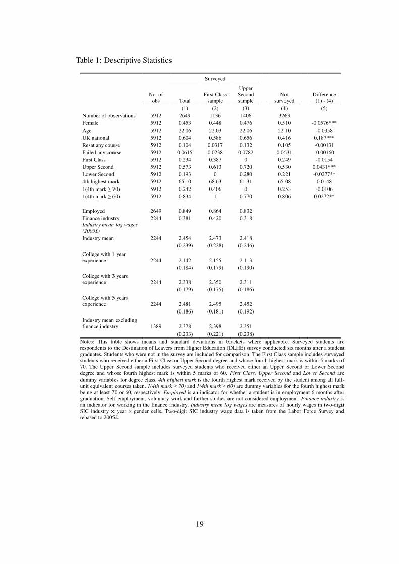
Table 1: Descriptive Statistics

Surveyed

No. of

obs Total

First Class

sample

Upper

Second

sample

Not

surveyed

Difference

(1) - (4)

(1) (2) (3) (4) (5)

Number of observations 5912 2649 1136 1406 3263

Female 5912 0.453 0.448 0.476 0.510 -0.0576***

Age 5912 22.06 22.03 22.06 22.10 -0.0358

UK national 5912 0.604 0.586 0.656 0.416 0.187***

Resat any course 5912 0.104 0.0317 0.132 0.105 -0.00131

Failed any course 5912 0.0615 0.0238 0.0782 0.0631 -0.00160

First Class 5912 0.234 0.387 0 0.249 -0.0154

Upper Second 5912 0.573 0.613 0.720 0.530 0.0431***

Lower Second 5912 0.193 0 0.280 0.221 -0.0277**

4th highest mark 5912 65.10 68.63 61.31 65.08 0.0148

1(4th mark ≥ 70) 5912 0.242 0.406 0 0.253 -0.0106

1(4th mark ≥ 60) 5912 0.834 1 0.770 0.806 0.0272**

Employed 2649 0.849 0.864 0.832

Finance industry 2244 0.381 0.420 0.318

Industry mean log wages

(2005£)

Industry mean 2244 2.454 2.473 2.418

(0.239) (0.228) (0.246)

College with 1 year

experience 2244 2.142 2.155 2.113

(0.184) (0.179) (0.190)

College with 3 years

experience 2244 2.338 2.350 2.311

(0.179) (0.175) (0.186)

College with 5 years

experience 2244 2.481 2.495 2.452

(0.186) (0.181) (0.192)

Industry mean excluding

finance industry 1389 2.378 2.398 2.351

(0.233) (0.221) (0.238)

Notes: This table shows means and standard deviations in brackets where applicable. Surveyed students are

respondents to the Destination of Leavers from Higher Education (DLHE) survey conducted six months after a student

graduates. Students who were not in the survey are included for comparison. The First Class sample includes surveyed

students who received either a First Class or Upper Second degree and whose fourth highest mark is within 5 marks of

70. The Upper Second sample includes surveyed students who received either an Upper Second or Lower Second

degree and whose fourth highest mark is within 5 marks of 60. First Class, Upper Second and Lower Second are

dummy variables for degree class. 4th highest mark is the fourth highest mark received by the student among all full-

unit equivalent courses taken. 1(4th mark ≥ 70) and 1(4th mark ≥ 60) are dummy variables for the fourth highest mark

being at least 70 or 60, respectively. Employed is an indicator for whether a student is in employment 6 months after

graduation. Self-employment, voluntary work and further studies are not considered employment. Finance industry is

an indicator for working in the finance industry. Industry mean log wages are measures of hourly wages in two-digit

SIC industry × year × gender cells. Two-digit SIC industry wage data is taken from the Labor Force Survey and

rebased to 2005£.

19

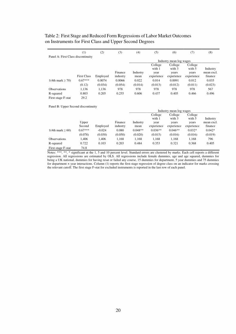
Table 2: First Stage and Reduced Form Regressions of Labor Market Outcomeson Instruments for First Class and Upper Second Degrees

(1) (2) (3) (4) (5) (6) (7) (8)

Panel A: First Class discontinuity

Industry mean log wages

First Class Employed

Finance

industry

Industry

mean

College

with 1

year

experience

College

with 3

years

experience

College

with 5

years

experience

Industry

mean excl.

finance

1(4th mark ≥ 70) 0.67*** 0.0074 0.0066 0.022 0.014 0.0091 0.012 0.035

(0.12) (0.034) (0.054) (0.014) (0.013) (0.012) (0.011) (0.023)

Observations 1,136 1,136 978 978 978 978 978 567

R-squared 0.803 0.205 0.255 0.606 0.437 0.405 0.466 0.496

First-stage F-stat 29.2

Panel B: Upper Second discontinuity

Industry mean log wages

Upper

Second Employed

Finance

industry

Industry

mean

College

with 1

year

experience

College

with 3

years

experience

College

with 5

years

experience

Industry

mean excl.

finance

1(4th mark ≥ 60) 0.67*** -0.024 0.080 0.048** 0.036** 0.046** 0.032* 0.042*

(0.078) (0.030) (0.050) (0.020) (0.015) (0.016) (0.016) (0.019)

Observations 1,406 1,406 1,168 1,168 1,168 1,168 1,168 796

R-squared 0.722 0.103 0.203 0.484 0.353 0.321 0.368 0.405

First-stage F-stat 74.8

Notes: ***, **, * significant at the 1, 5 and 10 percent level. Standard errors are clustered by marks. Each cell reports a different

regression. All regressions are estimated by OLS. All regressions include female dummies, age and age squared, dummies for

being a UK national, dummies for having resat or failed any course, 15 dummies for department, 5 year dummies and 75 dummies

for department × year interactions. Column (1) reports the first-stage regression of degree class on an indicator for marks crossing

the relevant cutoff. The first stage F-stat for excluded instruments is reported in the last row of each panel.

20

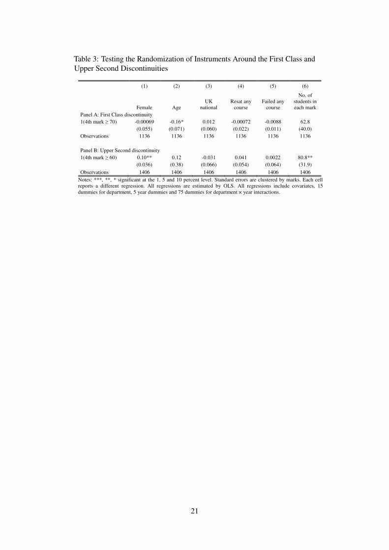
Table 3: Testing the Randomization of Instruments Around the First Class andUpper Second Discontinuities

(1) (2) (3) (4) (5) (6)

Female Age

UK

national

Resat any

course

Failed any

course

No. of

students in

each mark

Panel A: First Class discontinuity

1(4th mark ≥ 70) -0.00069 -0.16* 0.012 -0.00072 -0.0088 62.8

(0.055) (0.071) (0.060) (0.022) (0.011) (40.0)

Observations 1136 1136 1136 1136 1136 1136

Panel B: Upper Second discontinuity

1(4th mark ≥ 60) 0.10** 0.12 -0.031 0.041 0.0022 80.8**

(0.036) (0.38) (0.066) (0.054) (0.064) (31.9)

Observations 1406 1406 1406 1406 1406 1406

Notes: ***, **, * significant at the 1, 5 and 10 percent level. Standard errors are clustered by marks. Each cell

reports a different regression. All regressions are estimated by OLS. All regressions include covariates, 15

dummies for department, 5 year dummies and 75 dummies for department × year interactions.

21

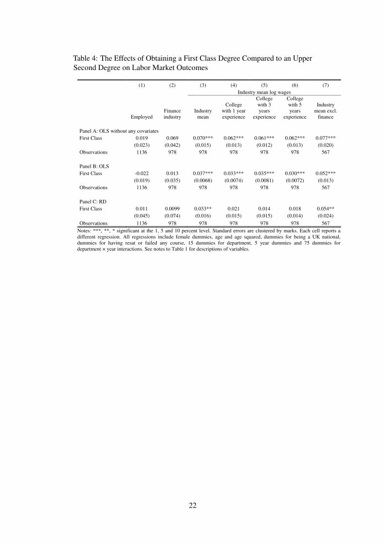
Table 4: The Effects of Obtaining a First Class Degree Compared to an UpperSecond Degree on Labor Market Outcomes

(1) (2) (3) (4) (5) (6) (7)

Industry mean log wages

Employed

Finance

industry

Industry

mean

College

with 1 year

experience

College

with 3

years

experience

College

with 5

years

experience

Industry

mean excl.

finance

Panel A: OLS without any covariates

First Class 0.019 0.069 0.070*** 0.062*** 0.061*** 0.062*** 0.077***

(0.023) (0.042) (0.015) (0.013) (0.012) (0.013) (0.020)

Observations 1136 978 978 978 978 978 567

Panel B: OLS

First Class -0.022 0.013 0.037*** 0.033*** 0.035*** 0.030*** 0.052***

(0.019) (0.035) (0.0068) (0.0074) (0.0081) (0.0072) (0.013)

Observations 1136 978 978 978 978 978 567

Panel C: RD

First Class 0.011 0.0099 0.033** 0.021 0.014 0.018 0.054**

(0.045) (0.074) (0.016) (0.015) (0.015) (0.014) (0.024)

Observations 1136 978 978 978 978 978 567

Notes: ***, **, * significant at the 1, 5 and 10 percent level. Standard errors are clustered by marks. Each cell reports a

different regression. All regressions include female dummies, age and age squared, dummies for being a UK national,

dummies for having resat or failed any course, 15 dummies for department, 5 year dummies and 75 dummies for

department × year interactions. See notes to Table 1 for descriptions of variables.

22

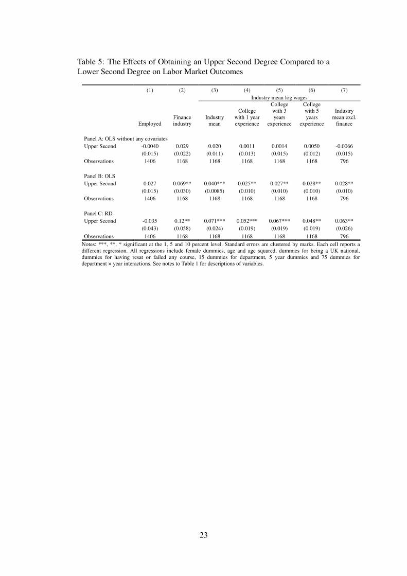
Table 5: The Effects of Obtaining an Upper Second Degree Compared to aLower Second Degree on Labor Market Outcomes

(1) (2) (3) (4) (5) (6) (7)

Industry mean log wages

Employed

Finance

industry

Industry

mean

College

with 1 year

experience

College

with 3

years

experience

College

with 5

years

experience

Industry

mean excl.

finance

Panel A: OLS without any covariates

Upper Second -0.0040 0.029 0.020 0.0011 0.0014 0.0050 -0.0066

(0.015) (0.022) (0.011) (0.013) (0.015) (0.012) (0.015)

Observations 1406 1168 1168 1168 1168 1168 796

Panel B: OLS

Upper Second 0.027 0.069** 0.040*** 0.025** 0.027** 0.028** 0.028**

(0.015) (0.030) (0.0085) (0.010) (0.010) (0.010) (0.010)

Observations 1406 1168 1168 1168 1168 1168 796

Panel C: RD

Upper Second -0.035 0.12** 0.071*** 0.052*** 0.067*** 0.048** 0.063**

(0.043) (0.058) (0.024) (0.019) (0.019) (0.019) (0.026)

Observations 1406 1168 1168 1168 1168 1168 796

Notes: ***, **, * significant at the 1, 5 and 10 percent level. Standard errors are clustered by marks. Each cell reports a

different regression. All regressions include female dummies, age and age squared, dummies for being a UK national,

dummies for having resat or failed any course, 15 dummies for department, 5 year dummies and 75 dummies for

department × year interactions. See notes to Table 1 for descriptions of variables.

23

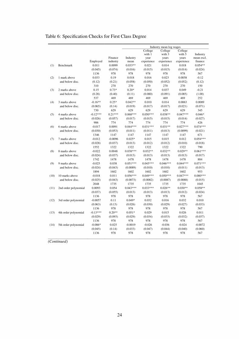
Table 6: Specification Checks for First Class Degree

Industry mean log wages

Employed

Finance

industry

Industry

mean

College

with 1

year

experience

College

with 3

years

experience

College

with 5

years

experience

Industry

mean excl.

finance

(1) Benchmark 0.011 0.0099 0.033** 0.021 0.014 0.018 0.054**

(0.045) (0.074) (0.016) (0.015) (0.015) (0.014) (0.024)

1136 978 978 978 978 978 567

(2) 1 mark above 0.033 0.19 0.018 0.016 0.023 0.0058 -0.12

and below disc. (0.12) (0.21) (0.058) (0.050) (0.052) (0.052) (0.12)

310 270 270 270 270 270 150

(3) 2 marks above 0.15 0.73* 0.20* 0.014 0.037 0.049 -0.21

and below disc. (0.28) (0.40) (0.11) (0.080) (0.091) (0.085) (1.00)

537 469 469 469 469 469 252

(4) 3 marks above -0.16** 0.25* 0.042** 0.010 0.014 0.0063 0.0089

and below disc. (0.065) (0.14) (0.019) (0.017) (0.017) (0.021) (0.071)

730 629 629 629 629 629 345

(5) 4 marks above -0.12*** 0.21*** 0.068*** 0.050*** 0.038** 0.047*** 0.046*

and below disc. (0.026) (0.057) (0.017) (0.015) (0.015) (0.014) (0.027)

906 774 774 774 774 774 426

(6) 6 marks above -0.017 0.0091 0.044*** 0.031*** 0.031** 0.027*** 0.074***

and below disc. (0.030) (0.053) (0.011) (0.011) (0.013) (0.0099) (0.021)

1346 1147 1147 1147 1147 1147 671

(7) 7 marks above -0.012 -0.0096 0.025* 0.015 0.015 0.012 0.054***

and below disc. (0.028) (0.037) (0.013) (0.012) (0.012) (0.010) (0.018)

1552 1322 1322 1322 1322 1322 790

(8) 8 marks above -0.022 0.0048 0.038*** 0.032** 0.032** 0.029** 0.061***

and below disc. (0.024) (0.037) (0.013) (0.013) (0.013) (0.013) (0.017)

1742 1478 1478 1478 1478 1478 884

(9) 9 marks above -0.025 0.038 0.051*** 0.045*** 0.046*** 0.044*** 0.071***

and below disc. (0.024) (0.043) (0.0089) (0.010) (0.010) (0.011) (0.013)

1894 1602 1602 1602 1602 1602 953

(10) 10 marks above -0.018 0.011 0.056*** 0.049*** 0.050*** 0.047*** 0.080***

and below disc. (0.025) (0.043) (0.0073) (0.0082) (0.0087) (0.0088) (0.015)

2048 1735 1735 1735 1735 1735 1045

(11) 2nd order polynomial 0.0093 0.054 0.043*** 0.033*** 0.026** 0.030** 0.058**

(0.037) (0.055) (0.013) (0.013) (0.013) (0.012) (0.024)

1136 978 978 978 978 978 567

(12) 3rd order polynomial -0.0057 0.11 0.049* 0.032 0.016 0.032 0.010

(0.063) (0.13) (0.026) (0.030) (0.029) (0.027) (0.033)

1136 978 978 978 978 978 567

(13) 4th order polynomial -0.13*** 0.20** 0.051* 0.029 0.015 0.026 0.011

(0.029) (0.093) (0.029) (0.034) (0.033) (0.032) (0.037)

1136 978 978 978 978 978 567

(14) 5th order polynomial -0.086* 0.025 -0.0019 -0.026 -0.036 -0.024 -0.0072

(0.045) (0.14) (0.033) (0.047) (0.044) (0.040) (0.060)

1136 978 978 978 978 978 567

(Continued)

24

Industry mean log wages

Employed

Finance

industry

Industry

mean

College

with 1

year

experience

College

with 3

years

experience

College

with 5

years

experience

Industry

mean excl.

finance

(14) Including controls 0.0095 0.0096 0.032** 0.020 0.013 0.017 0.052**

for sum of marks (0.044) (0.073) (0.015) (0.015) (0.015) (0.013) (0.022)

1136 978 978 978 978 978 567

(15) Including controls 0.011 0.021 0.034** 0.024 0.017 0.020 0.051**

for other marks (0.045) (0.073) (0.015) (0.015) (0.015) (0.014) (0.023)

1136 978 978 978 978 978 567

(16) UK domicile sample -0.015 0.14 0.031 0.047** 0.035* 0.039** -0.0072

(0.063) (0.094) (0.025) (0.021) (0.020) (0.019) (0.040)

701 585 585 585 585 585 367

(17) Excluding marks -0.0016 0.0078 0.048*** 0.035** 0.036*** 0.028** 0.078***

around disc. (0.062) (0.094) (0.011) (0.014) (0.012) (0.012) (0.017)

922 791 791 791 791 791 462

Notes: ***, **, * significant at the 1, 5 and 10 percent level. Standard errors are clustered by marks. This table reports specification

checks of the benchmark model in Table 4, panel C. Each cell reports a different regression where the coefficients on First Class

are reported in the first lines, standard errors in brackets and number of observations in the third lines.

25

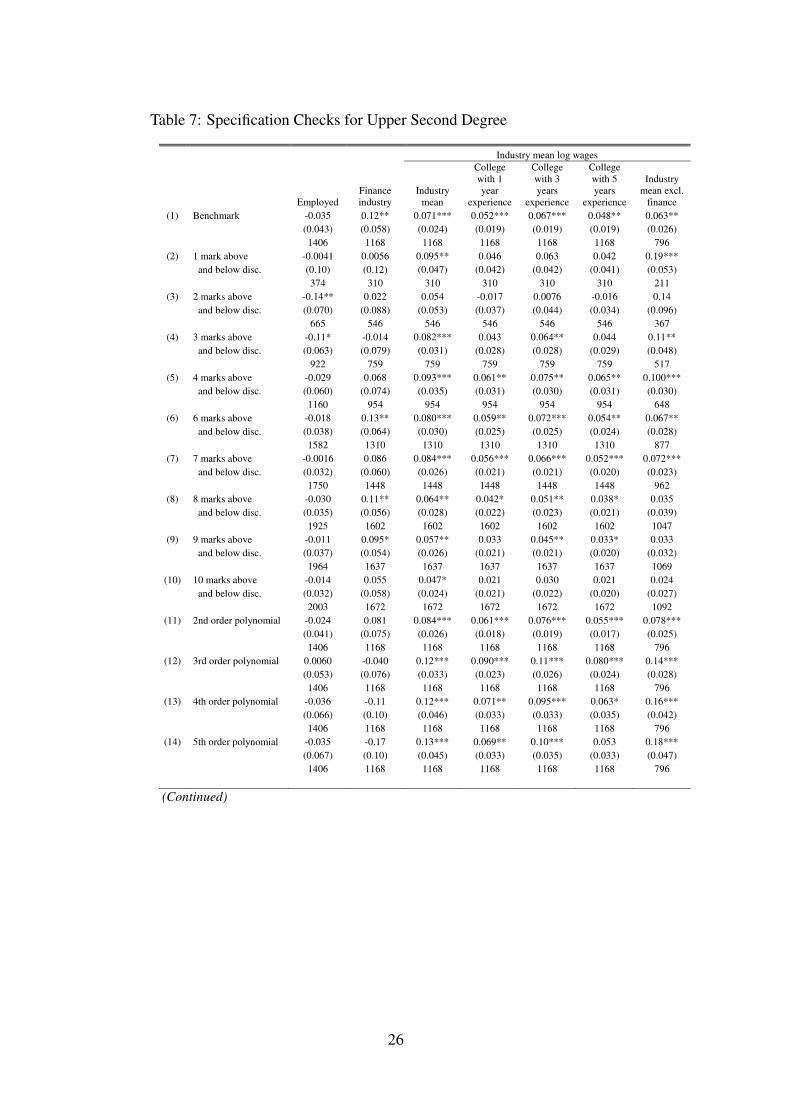
Table 7: Specification Checks for Upper Second Degree

Industry mean log wages

Employed

Finance

industry

Industry

mean

College

with 1

year

experience

College

with 3

years

experience

College

with 5

years

experience

Industry

mean excl.

finance

(1) Benchmark -0.035 0.12** 0.071*** 0.052*** 0.067*** 0.048** 0.063**

(0.043) (0.058) (0.024) (0.019) (0.019) (0.019) (0.026)

1406 1168 1168 1168 1168 1168 796

(2) 1 mark above -0.0041 0.0056 0.095** 0.046 0.063 0.042 0.19***

and below disc. (0.10) (0.12) (0.047) (0.042) (0.042) (0.041) (0.053)

374 310 310 310 310 310 211

(3) 2 marks above -0.14** 0.022 0.054 -0.017 0.0076 -0.016 0.14

and below disc. (0.070) (0.088) (0.053) (0.037) (0.044) (0.034) (0.096)

665 546 546 546 546 546 367

(4) 3 marks above -0.11* -0.014 0.082*** 0.043 0.064** 0.044 0.11**

and below disc. (0.063) (0.079) (0.031) (0.028) (0.028) (0.029) (0.048)

922 759 759 759 759 759 517

(5) 4 marks above -0.029 0.068 0.093*** 0.061** 0.075** 0.065** 0.100***

and below disc. (0.060) (0.074) (0.035) (0.031) (0.030) (0.031) (0.030)

1160 954 954 954 954 954 648

(6) 6 marks above -0.018 0.13** 0.080*** 0.059** 0.072*** 0.054** 0.067**

and below disc. (0.038) (0.064) (0.030) (0.025) (0.025) (0.024) (0.028)

1582 1310 1310 1310 1310 1310 877

(7) 7 marks above -0.0016 0.086 0.084*** 0.056*** 0.066*** 0.052*** 0.072***

and below disc. (0.032) (0.060) (0.026) (0.021) (0.021) (0.020) (0.023)

1750 1448 1448 1448 1448 1448 962

(8) 8 marks above -0.030 0.11** 0.064** 0.042* 0.051** 0.038* 0.035

and below disc. (0.035) (0.056) (0.028) (0.022) (0.023) (0.021) (0.039)

1925 1602 1602 1602 1602 1602 1047

(9) 9 marks above -0.011 0.095* 0.057** 0.033 0.045** 0.033* 0.033

and below disc. (0.037) (0.054) (0.026) (0.021) (0.021) (0.020) (0.032)

1964 1637 1637 1637 1637 1637 1069

(10) 10 marks above -0.014 0.055 0.047* 0.021 0.030 0.021 0.024

and below disc. (0.032) (0.058) (0.024) (0.021) (0.022) (0.020) (0.027)

2003 1672 1672 1672 1672 1672 1092

(11) 2nd order polynomial -0.024 0.081 0.084*** 0.061*** 0.076*** 0.055*** 0.078***

(0.041) (0.075) (0.026) (0.018) (0.019) (0.017) (0.025)

1406 1168 1168 1168 1168 1168 796

(12) 3rd order polynomial 0.0060 -0.040 0.12*** 0.090*** 0.11*** 0.080*** 0.14***

(0.053) (0.076) (0.033) (0.023) (0.026) (0.024) (0.028)

1406 1168 1168 1168 1168 1168 796

(13) 4th order polynomial -0.036 -0.11 0.12*** 0.071** 0.095*** 0.063* 0.16***

(0.066) (0.10) (0.046) (0.033) (0.033) (0.035) (0.042)

1406 1168 1168 1168 1168 1168 796

(14) 5th order polynomial -0.035 -0.17 0.13*** 0.069** 0.10*** 0.053 0.18***

(0.067) (0.10) (0.045) (0.033) (0.035) (0.033) (0.047)

1406 1168 1168 1168 1168 1168 796

(Continued)

26

Industry mean log wages

Employed

Finance

industry

Industry

mean

College

with 1

year

experience

College

with 3

years

experience

College

with 5

years

experience

Industry

mean excl.

finance

(14) Including controls -0.037 0.11* 0.065** 0.047** 0.063*** 0.043** 0.060**

for sum of marks (0.042) (0.059) (0.026) (0.020) (0.020) (0.020) (0.027)

1406 1168 1168 1168 1168 1168 796

(15) Including controls -0.043 0.12* 0.071*** 0.052*** 0.067*** 0.046** 0.062**

for other marks (0.051) (0.060) (0.026) (0.020) (0.020) (0.020) (0.027)

1406 1168 1168 1168 1168 1168 796

(16) UK domicile sample -0.083* 0.033 0.091*** 0.076*** 0.087*** 0.064*** 0.10***

(0.042) (0.059) (0.023) (0.021) (0.023) (0.022) (0.032)

974 792 792 792 792 792 574

(17) Excluding marks -0.036 0.21*** 0.077*** 0.055*** 0.068*** 0.056*** 0.055*

around disc. (0.040) (0.033) (0.022) (0.015) (0.014) (0.017) (0.029)

1182 978 978 978 978 978 654

Notes: ***, **, * significant at the 1, 5 and 10 percent level. Standard errors are clustered by marks. This table reports

specification checks of the benchmark model in Table 5, panel C. Each cell reports a different regression where the coefficients

on Upper Second are reported in the first lines, standard errors in brackets and number of observations in the third lines.

27

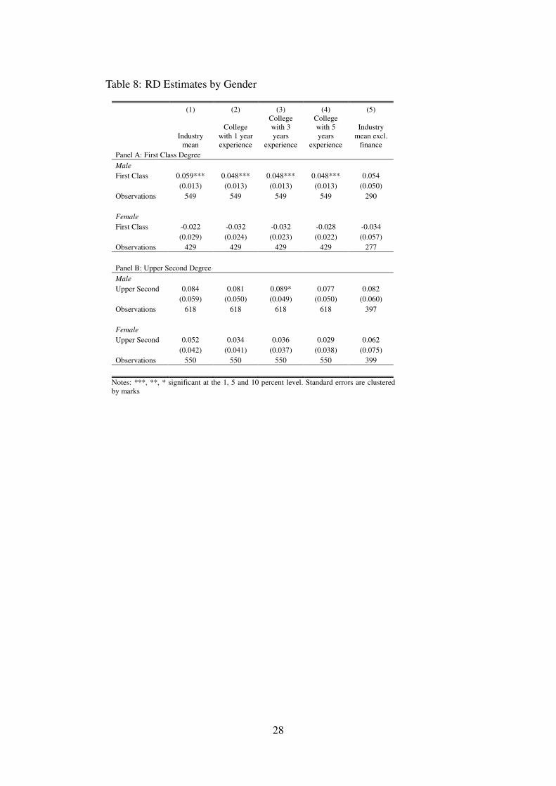
Table 8: RD Estimates by Gender

(1) (2) (3) (4) (5)

Industry

mean

College

with 1 year

experience

College

with 3

years

experience

College

with 5

years

experience

Industry

mean excl.

finance

Panel A: First Class Degree

Male

First Class 0.059*** 0.048*** 0.048*** 0.048*** 0.054

(0.013) (0.013) (0.013) (0.013) (0.050)

Observations 549 549 549 549 290

Female

First Class -0.022 -0.032 -0.032 -0.028 -0.034

(0.029) (0.024) (0.023) (0.022) (0.057)

Observations 429 429 429 429 277

Panel B: Upper Second Degree

Male

Upper Second 0.084 0.081 0.089* 0.077 0.082

(0.059) (0.050) (0.049) (0.050) (0.060)

Observations 618 618 618 618 397

Female

Upper Second 0.052 0.034 0.036 0.029 0.062

(0.042) (0.041) (0.037) (0.038) (0.075)

Observations 550 550 550 550 399

Notes: ***, **, * significant at the 1, 5 and 10 percent level. Standard errors are clustered

by marks

28

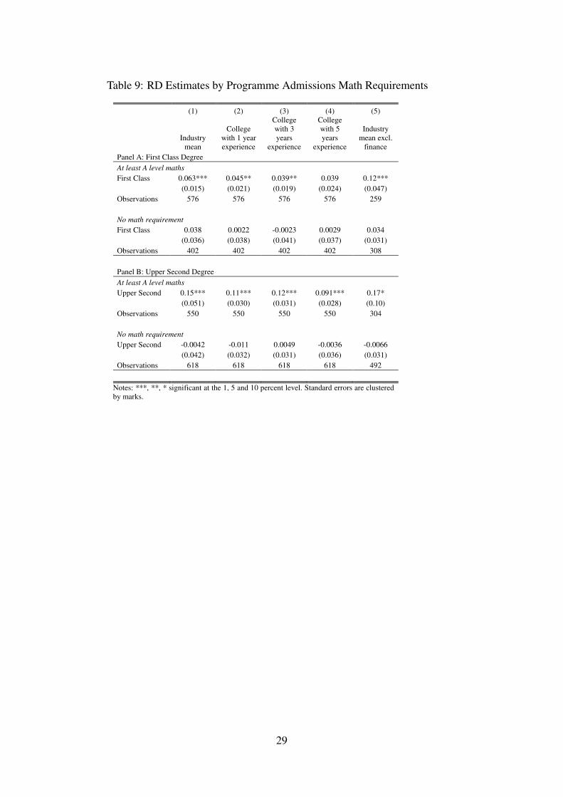
Table 9: RD Estimates by Programme Admissions Math Requirements

(1) (2) (3) (4) (5)

Industry

mean

College

with 1 year

experience

College

with 3

years

experience

College

with 5

years

experience

Industry

mean excl.

finance

Panel A: First Class Degree

At least A level maths

First Class 0.063*** 0.045** 0.039** 0.039 0.12***

(0.015) (0.021) (0.019) (0.024) (0.047)

Observations 576 576 576 576 259

No math requirement

First Class 0.038 0.0022 -0.0023 0.0029 0.034

(0.036) (0.038) (0.041) (0.037) (0.031)

Observations 402 402 402 402 308

Panel B: Upper Second Degree

At least A level maths

Upper Second 0.15*** 0.11*** 0.12*** 0.091*** 0.17*

(0.051) (0.030) (0.031) (0.028) (0.10)

Observations 550 550 550 550 304

No math requirement

Upper Second -0.0042 -0.011 0.0049 -0.0036 -0.0066

(0.042) (0.032) (0.031) (0.036) (0.031)

Observations 618 618 618 618 492

Notes: ***, **, * significant at the 1, 5 and 10 percent level. Standard errors are clustered

by marks.

29

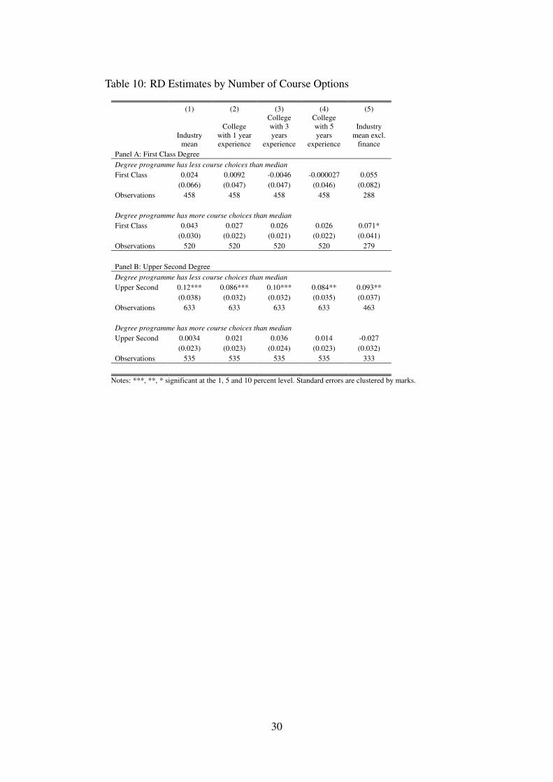
Table 10: RD Estimates by Number of Course Options

(1) (2) (3) (4) (5)

Industry

mean

College

with 1 year

experience

College

with 3

years

experience

College

with 5

years

experience

Industry

mean excl.

finance

Panel A: First Class Degree

Degree programme has less course choices than median

First Class 0.024 0.0092 -0.0046 -0.000027 0.055

(0.066) (0.047) (0.047) (0.046) (0.082)

Observations 458 458 458 458 288

Degree programme has more course choices than median

First Class 0.043 0.027 0.026 0.026 0.071*

(0.030) (0.022) (0.021) (0.022) (0.041)

Observations 520 520 520 520 279

Panel B: Upper Second Degree

Degree programme has less course choices than median

Upper Second 0.12*** 0.086*** 0.10*** 0.084** 0.093**

(0.038) (0.032) (0.032) (0.035) (0.037)

Observations 633 633 633 633 463

Degree programme has more course choices than median

Upper Second 0.0034 0.021 0.036 0.014 -0.027

(0.023) (0.023) (0.024) (0.023) (0.032)

Observations 535 535 535 535 333

Notes: ***, **, * significant at the 1, 5 and 10 percent level. Standard errors are clustered by marks.

30

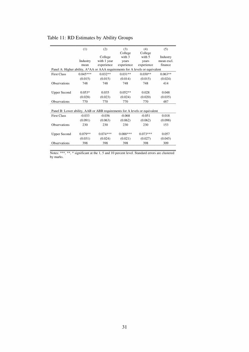
Table 11: RD Estimates by Ability Groups

(1) (2) (3) (4) (5)

Industry

mean

College

with 1 year

experience

College

with 3

years

experience

College

with 5

years

experience

Industry

mean excl.

finance

Panel A: Higher ability, A*AA or AAA requirements for A levels or equivalent

First Class 0.045*** 0.032** 0.031** 0.030** 0.063**

(0.015) (0.015) (0.014) (0.015) (0.024)

Observations 748 748 748 748 414

Upper Second 0.053* 0.035 0.052** 0.028 0.048

(0.028) (0.023) (0.024) (0.020) (0.035)

Observations 770 770 770 770 487

Panel B: Lower ability, AAB or ABB requirements for A levels or equivalent

First Class -0.033 -0.036 -0.068 -0.051 0.018

(0.091) (0.063) (0.062) (0.062) (0.098)

Observations 230 230 230 230 153

Upper Second 0.079** 0.074*** 0.088*** 0.073*** 0.057

(0.031) (0.024) (0.021) (0.027) (0.045)

Observations 398 398 398 398 309

Notes: ***, **, * significant at the 1, 5 and 10 percent level. Standard errors are clustered

by marks.

31

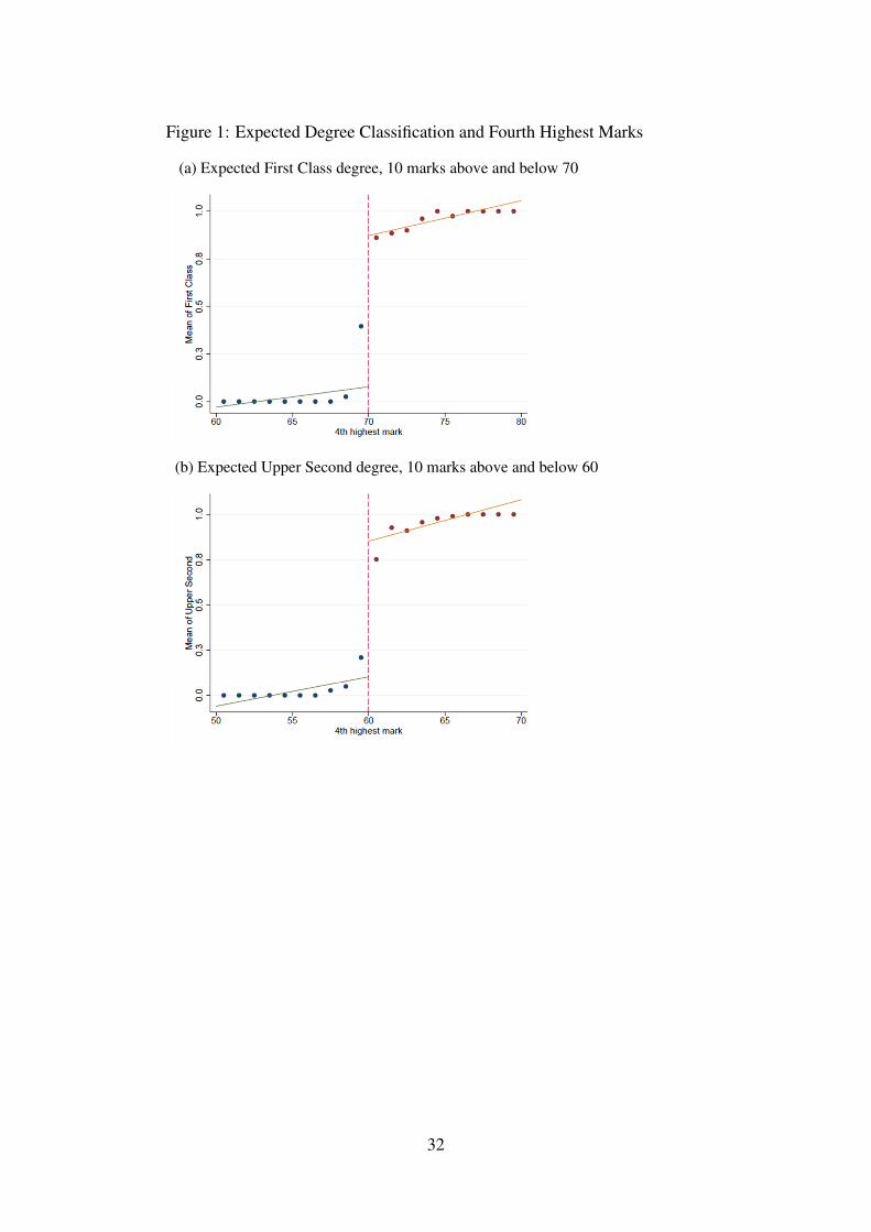
Figure 1: Expected Degree Classification and Fourth Highest Marks

(a) Expected First Class degree, 10 marks above and below 70

(b) Expected Upper Second degree, 10 marks above and below 60

32

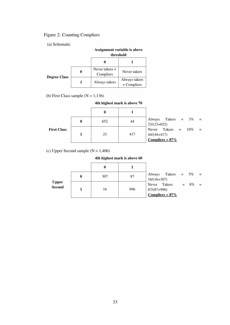
Figure 2: Counting Compliers

(a) Schematic

Assignment variable is above

threshold

0 1

Degree Class

0 Never takers +

Compliers Never takers

1 Always takers Always takers

+ Compliers

(b) First Class sample (N = 1,136)

4th highest mark is above 70

0 1

First Class

0 652 44 Always Takers = 3% =

23/(23+652)

Never Takers = 10% =

44/(44+417)

Compliers = 87%

1 23 417

(c) Upper Second sample (N = 1,406)

4th highest mark is above 60

0 1

Upper

Second

0 307 87 Always Takers = 5% =

16/(16+307)

Never Takers = 8% =

87/(87+996)

Compliers = 87%

1 16 996

33

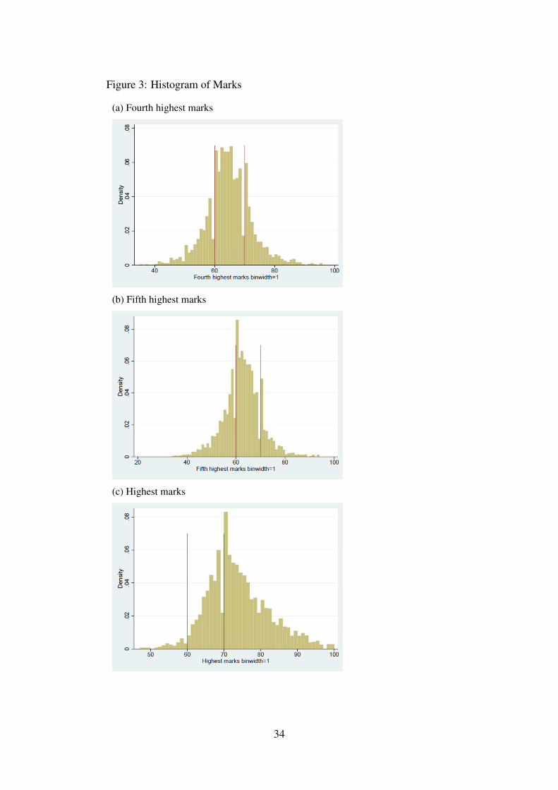
Figure 3: Histogram of Marks

(a) Fourth highest marks

(b) Fifth highest marks

(c) Highest marks

34

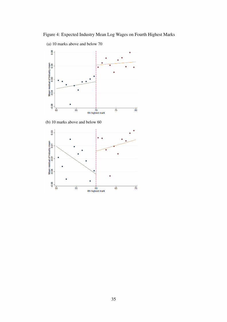
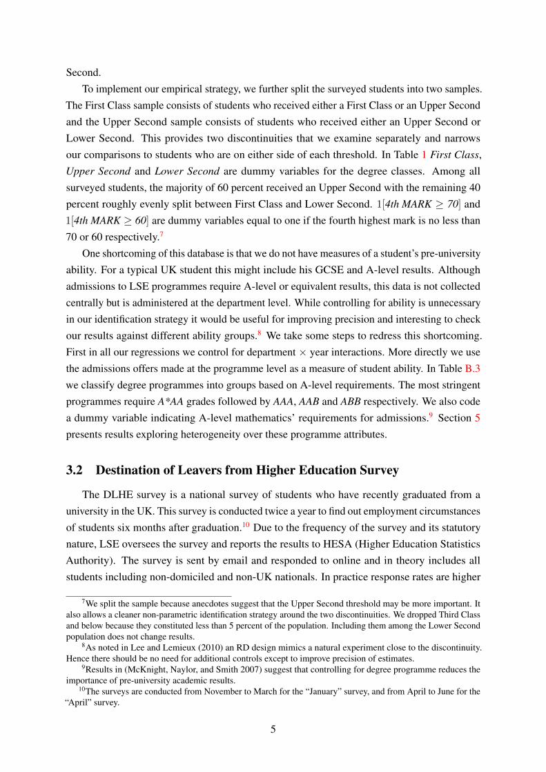
Figure 4: Expected Industry Mean Log Wages on Fourth Highest Marks

(a) 10 marks above and below 70

(b) 10 marks above and below 60

35

Appendices

A Simple Model of Statistical Discrimination

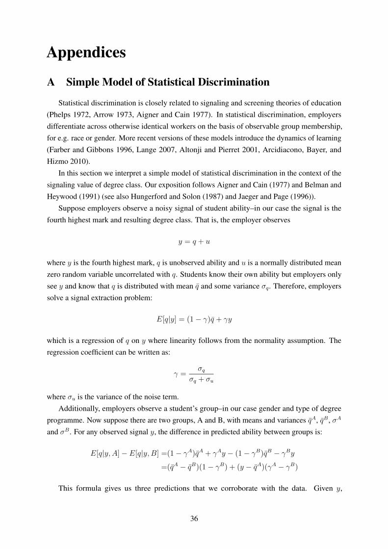
Statistical discrimination is closely related to signaling and screening theories of education(Phelps 1972, Arrow 1973, Aigner and Cain 1977). In statistical discrimination, employersdifferentiate across otherwise identical workers on the basis of observable group membership,for e.g. race or gender. More recent versions of these models introduce the dynamics of learning(Farber and Gibbons 1996, Lange 2007, Altonji and Pierret 2001, Arcidiacono, Bayer, andHizmo 2010).

In this section we interpret a simple model of statistical discrimination in the context of thesignaling value of degree class. Our exposition follows Aigner and Cain (1977) and Belman andHeywood (1991) (see also Hungerford and Solon (1987) and Jaeger and Page (1996)).

Suppose employers observe a noisy signal of student ability–in our case the signal is thefourth highest mark and resulting degree class. That is, the employer observes

y = q + u

where y is the fourth highest mark, q is unobserved ability and u is a normally distributed meanzero random variable uncorrelated with q. Students know their own ability but employers onlysee y and know that q is distributed with mean q̄ and some variance σq. Therefore, employerssolve a signal extraction problem:

E[q|y] = (1− γ)q̄ + γy

which is a regression of q on y where linearity follows from the normality assumption. Theregression coefficient can be written as:

γ =σq

σq + σu

where σu is the variance of the noise term.Additionally, employers observe a student’s group–in our case gender and type of degree

programme. Now suppose there are two groups, A and B, with means and variances q̄A, q̄B , σA

and σB. For any observed signal y, the difference in predicted ability between groups is:

E[q|y, A]− E[q|y,B] =(1− γA)q̄A + γAy − (1− γB)q̄B − γBy

=(q̄A − q̄B)(1− γB) + (y − q̄A)(γA − γB)

This formula gives us three predictions that we corroborate with the data. Given y,

36

E[q|y, A]− E[q|y,B] > 0, if

1. q̄A − q̄B > 0

2. σAq − σB

q > 0 and y > q̄

3. σAu − σB

u < 0 and y > q̄.

In the data we interpret y as the fourth highest mark so q̄ = E[y]. The total variance can becalculated as σy = σq +σu but we do not observe σq or σu separately. Because we do not observeσu we cannot recover the exact importance of each factor in determining group differences. Ourapplication of the model to the data should necessarily be interpreted loosely. When we translatethe predictions to the data, at any given mark and degree class, a student from group A has ahigher predicted ability than an otherwise identical student from group B if group A has:

1. higher expected abilities;

2. higher variance in abilities and y is a positive signal;

3. lower variance in the noise term and y is a positive signal.

In our context, a positive signal is receipt of the higher degree class. Both First Class andUpper Second are positive signals because we are always comparing to the next lower class. Asdiscussed in Section 5.1 we define groups by gender and degree programmes and find resultssupportive of this simple model statistical discrimination.

37

B Appendix Tables

38

Table B.1: Mapping From Course Marks to Final Degree Class

Final degree class Course grade requirements

First Class Honors 5 marks of 70 or above or

4 marks of 70 or above and aggregate marks of at least 590

Upper Second Class 5 marks of 60 or above or

4 marks of 60 or above and aggregate marks of at least 515

Lower Second Class 5 marks of 50 or above or

4 marks of 50 or above and aggregate marks of at least 440

Notes: Institutional rules governing award of degree class taken from

http://www.lse.ac.uk/resources/calendar/academicRegulations/BA-BScDegrees.htm

39

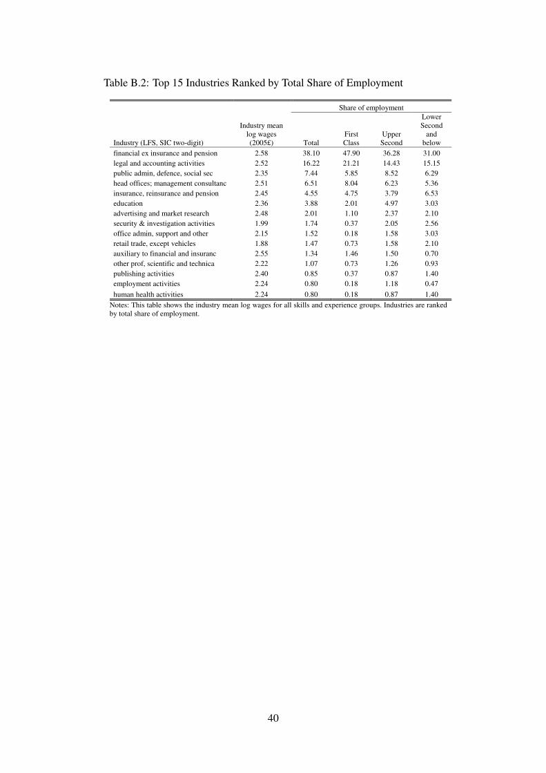
Table B.2: Top 15 Industries Ranked by Total Share of Employment

Share of employment

Industry (LFS, SIC two-digit)

Industry mean

log wages

(2005£) Total

First

Class

Upper

Second

Lower

Second

and

below

financial ex insurance and pension 2.58 38.10 47.90 36.28 31.00

legal and accounting activities 2.52 16.22 21.21 14.43 15.15

public admin, defence, social sec 2.35 7.44 5.85 8.52 6.29

head offices; management consultanc 2.51 6.51 8.04 6.23 5.36

insurance, reinsurance and pension 2.45 4.55 4.75 3.79 6.53

education 2.36 3.88 2.01 4.97 3.03

advertising and market research 2.48 2.01 1.10 2.37 2.10

security & investigation activities 1.99 1.74 0.37 2.05 2.56

office admin, support and other 2.15 1.52 0.18 1.58 3.03

retail trade, except vehicles 1.88 1.47 0.73 1.58 2.10

auxiliary to financial and insuranc 2.55 1.34 1.46 1.50 0.70

other prof, scientific and technica 2.22 1.07 0.73 1.26 0.93

publishing activities 2.40 0.85 0.37 0.87 1.40

employment activities 2.24 0.80 0.18 1.18 0.47

human health activities 2.24 0.80 0.18 0.87 1.40

Notes: This table shows the industry mean log wages for all skills and experience groups. Industries are ranked

by total share of employment.

40

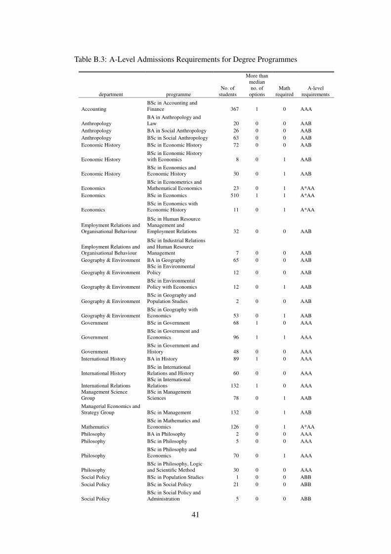
Table B.3: A-Level Admissions Requirements for Degree Programmes

department programme

No. of

students

More than

median

no. of

options

Math

required

A-level

requirements

Accounting

BSc in Accounting and

Finance 367 1 0 AAA

Anthropology

BA in Anthropology and

Law 20 0 0 AAB

Anthropology BA in Social Anthropology 26 0 0 AAB

Anthropology BSc in Social Anthropology 63 0 0 AAB

Economic History BSc in Economic History 72 0 0 AAB

Economic History

BSc in Economic History

with Economics 8 0 1 AAB

Economic History

BSc in Economics and

Economic History 30 0 1 AAB

Economics

BSc in Econometrics and

Mathematical Economics 23 0 1 A*AA

Economics BSc in Economics 510 1 1 A*AA

Economics

BSc in Economics with

Economic History 11 0 1 A*AA

Employment Relations and

Organisational Behaviour

BSc in Human Resource

Management and

Employment Relations 32 0 0 AAB

Employment Relations and

Organisational Behaviour

BSc in Industrial Relations

and Human Resource

Management 7 0 0 AAB

Geography & Environment BA in Geography 65 0 0 AAB

Geography & Environment

BSc in Environmental

Policy 12 0 0 AAB

Geography & Environment

BSc in Environmental

Policy with Economics 12 0 1 AAB

Geography & Environment

BSc in Geography and

Population Studies 2 0 0 AAB

Geography & Environment

BSc in Geography with

Economics 53 0 1 AAB

Government BSc in Government 68 1 0 AAA

Government

BSc in Government and

Economics 96 1 1 AAA

Government

BSc in Government and

History 48 0 0 AAA

International History BA in History 89 1 0 AAA

International History

BSc in International

Relations and History 60 0 0 AAA

International Relations

BSc in International

Relations 132 1 0 AAA

Management Science

Group

BSc in Management

Sciences 78 0 1 AAB

Managerial Economics and

Strategy Group BSc in Management 132 0 1 AAB

Mathematics

BSc in Mathematics and

Economics 126 0 1 A*AA

Philosophy BA in Philosophy 2 0 0 AAA

Philosophy BSc in Philosophy 5 0 0 AAA

Philosophy

BSc in Philosophy and

Economics 70 0 1 AAA

Philosophy

BSc in Philosophy, Logic

and Scientific Method 30 0 0 AAA

Social Policy BSc in Population Studies 1 0 0 ABB

Social Policy BSc in Social Policy 21 0 0 ABB

Social Policy

BSc in Social Policy and

Administration 5 0 0 ABB

41

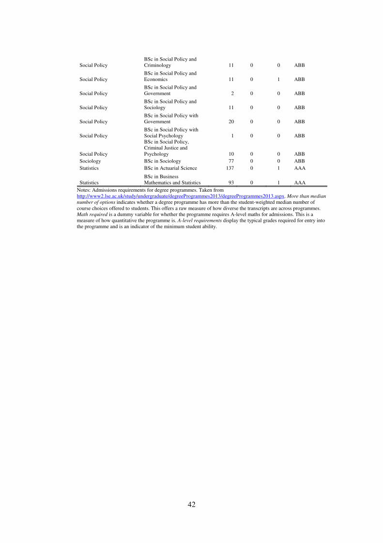
Social Policy

BSc in Social Policy and

Criminology 11 0 0 ABB

Social Policy

BSc in Social Policy and

Economics 11 0 1 ABB

Social Policy

BSc in Social Policy and

Government 2 0 0 ABB

Social Policy

BSc in Social Policy and

Sociology 11 0 0 ABB

Social Policy

BSc in Social Policy with

Government 20 0 0 ABB

Social Policy

BSc in Social Policy with

Social Psychology 1 0 0 ABB

Social Policy

BSc in Social Policy,

Criminal Justice and

Psychology 10 0 0 ABB

Sociology BSc in Sociology 77 0 0 ABB

Statistics BSc in Actuarial Science 137 0 1 AAA

Statistics

BSc in Business

Mathematics and Statistics 93 0 1 AAA

Notes: Admissions requirements for degree programmes. Taken from

http://www2.lse.ac.uk/study/undergraduate/degreeProgrammes2013/degreeProgrammes2013.aspx. More than median

number of options indicates whether a degree programme has more than the student-weighted median number of

course choices offered to students. This offers a raw measure of how diverse the transcripts are across programmes.

Math required is a dummy variable for whether the programme requires A-level maths for admissions. This is a

measure of how quantitative the programme is. A-level requirements display the typical grades required for entry into

the programme and is an indicator of the minimum student ability.

42

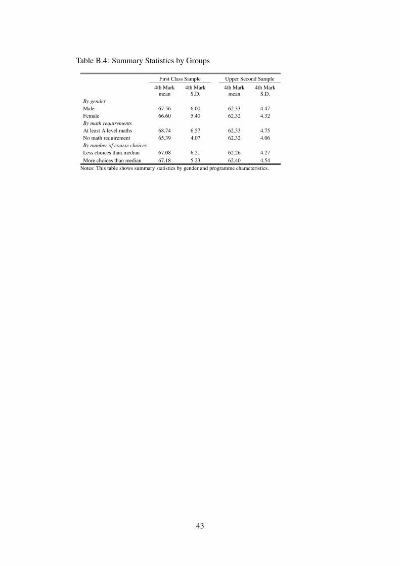
Table B.4: Summary Statistics by Groups

First Class Sample Upper Second Sample

4th Mark

mean

4th Mark

S.D.

4th Mark

mean

4th Mark

S.D.

By gender

Male 67.56 6.00 62.33 4.47

Female 66.60 5.40 62.32 4.32

By math requirements

At least A level maths 68.74 6.57 62.33 4.75

No math requirement 65.39 4.07 62.32 4.06

By number of course choices

Less choices than median 67.08 6.21 62.26 4.27

More choices than median 67.18 5.23 62.40 4.54

Notes: This table shows summary statistics by gender and programme characteristics.

43

Table B.5: Correlations Between Programme Level Measures

Mean

More than

median no.

of options

Math

required

A-level

score

A*AA or

AAA

More than median no. of

options 0.47 1.00

Math required 0.52 -0.09 1.00

A-level score A*AA or AAA 0.70 0.62 0.14 1.00

Notes: Each variable is a programme-level dummy variable described in detail in the

main text. This table shows mean and correlations weighted by number of students.

44

CENTRE FOR ECONOMIC PERFORMANCE

Recent Discussion Papers

1220 Esteban Aucejo Explaining Cross-Racial Differences in the

Educational Gender Gap

1219 Peter Arcidiacono

Esteban Aucejo

Andrew Hussey

Kenneth Spenner

Racial Segregation Patterns in Selective

Universities

1218 Silvana Tenreyro

Gregory Thwaites

Pushing On a String: US Monetary Policy is

Less Powerful in Recessions

1217 Gianluca Benigno

Luca Fornaro

The Financial Resource Curse

1216 Daron Acemoglu

Ufuk Akcigit

Nicholas Bloom

William R. Kerr

Innovation, Reallocation and Growth

1215 Michael J. Boehm Has Job Polarization Squeezed the Middle

Class? Evidence from the Allocation of

Talents

1214 Nattavudh Powdthavee

Warn N. Lekfuangfu

Mark Wooden

The Marginal Income Effect of Education on

Happiness: Estimating the Direct and Indirect

Effects of Compulsory Schooling on Well-

Being in Australia

1213 Richard Layard Mental Health: The New Frontier for Labour

Economics

1212 Francesco Caselli

Massimo Morelli

Dominic Rohner

The Geography of Inter-State Resource Wars

1211 Stephen Hansen

Michael McMahon

Estimating Bayesian Decision Problems with

Heterogeneous Priors

1210 Christopher A. Pissarides Unemployment in the Great Recession

1209 Kevin D. Sheedy Debt and Incomplete Financial Markets: A

Case for Nominal GDP Targeting

1208 Jordi Blanes i Vidal

Marc Möller

Decision-Making and Implementation in

Teams

1207 Michael J. Boehm Concentration versus Re-Matching? Evidence

About the Locational Effects of Commuting

Costs

1206 Antonella Nocco

Gianmarco I. P. Ottaviano

Matteo Salto

Monopolistic Competition and Optimum

Product Selection: Why and How

Heterogeneity Matters

1205 Alberto Galasso

Mark Schankerman

Patents and Cumulative Innovation: Causal

Evidence from the Courts

1204 L Rachel Ngai

Barbara Petrongolo

Gender Gaps and the Rise of the Service

Economy

1203 Luis Garicano

Luis Rayo

Relational Knowledge Transfers

1202 Abel Brodeur Smoking, Income and Subjective Well-Being:

Evidence from Smoking Bans

1201 Peter Boone

Ila Fazzio

Kameshwari Jandhyala

Chitra Jayanty

Gangadhar Jayanty

Simon Johnson

Vimala Ramachandrin

Filipa Silva

Zhaoguo Zhan

The Surprisingly Dire Situation of Children’s

Education in Rural West Africa: Results from

the CREO Study in Guinea-Bissau

1200 Marc J. Melitz

Stephen J. Redding

Firm Heterogeneity and Aggregate Welfare

1199 Giuseppe Berlingieri Outsourcing and the Rise in Services

1198 Sushil Wadhwani The Great Stagnation: What Can

Policymakers Do?

1197 Antoine Dechezleprêtre Fast-Tracking 'Green' Patent Applications:

An Empirical Analysis

1196 Abel Brodeur

Sarah Flèche

Where the Streets Have a Name: Income

Comparisons in the US

1195 Nicholas Bloom

Max Floetotto

Nir Jaimovich

Itay Saporta-Eksten

Stephen Terry

Really Uncertain Business Cycles

The Centre for Economic Performance Publications Unit

Tel 020 7955 7673 Fax 020 7404 0612

Email info@cep.lse.ac.uk Web site http://cep.lse.ac.uk