ISSN 2042-2695

CEP Discussion Paper No 1102

December 2011

A Note on Schooling in Development Accounting

Francesco Caselli and Antonio Ciccone

Abstract How much would output increase if underdeveloped economies were to increase their levels

of schooling? We contribute to the development accounting literature by describing a non-

parametric upper bound on the increase in output that can be generated by more schooling.

The advantage of our approach is that the upper bound is valid for any number of schooling

levels with arbitrary patterns of substitution/complementarity. We also quantify the upper

bound for all economies with the necessary data, compare our results with the standard

development accounting approach, and provide an update on the results using the standard

approach for a large sample of countries.

Keywords: schooling; production; efficiency; human capital; development accounting;

growth accounting

JEL Classifications: I28; J24

This paper was produced as part of the Centre’s Macro Programme. The Centre for Economic

Performance is financed by the Economic and Social Research Council.

Acknowledgements We thank Marcelo Soto, Hyun Son, and very especially David Weil for useful comments.

Francesco Caselli is a Programme Director at the Centre for Economic Performance

and Professor of Economics, London School of Economics. Antonio Ciccone is ICREA

Professor at the Universitat Pompeu Fabra. He is also Barcelona GSE Research Professor,

and research associate of CREI.

Published by

Centre for Economic Performance

London School of Economics and Political Science

Houghton Street

London WC2A 2AE

All rights reserved. No part of this publication may be reproduced, stored in a retrieval

system or transmitted in any form or by any means without the prior permission in writing of

the publisher nor be issued to the public or circulated in any form other than that in which it

is published. Requests for permission to reproduce any article or part of the Working Paper

should be sent to the editor at the above address.

F. Caselli and A. Ciccone, submitted 2011

1 Introduction

Low GDP per worker goes together with low schooling. For example, inthe country with the lowest output per worker in 2005, half the adultpopulation has no schooling at all and only 5% has a college degree(Barro and Lee, 2010). In the country with output per worker at the10th percentile, 32% of the population has no schooling and less than 1%a college degree. In the country at the 25th percentile, the populationshares without schooling and with a college degree are 22% and 1%respectively. On the other hand, in the US, the share of the populationwithout schooling is less than 0.5% and 16% have a college degree.How much of the output gap between developing and rich countries

can be accounted for by differences in the quantity of schooling? A ro-bust result in the development accounting literature, first establishedby Klenow and Rodriguez-Clare (1997) and Hall and Jones (1999), isthat only a relatively small fraction of the output gap between devel-oping and rich countries can be attributed to differences in the quan-tity of schooling. This result is obtained assuming that workers withdifferent levels of schooling are perfect substitutes in production (e.g.Klenow and Rodriguez-Clare, 1997; Hendricks, 2002). Perfect substitu-tion among different schooling levels is necessary to explain the absenceof large cross-country differences in the return to schooling if technologydifferences are assumed to be Hick-neutral.There is by now a consensus that differences in technology across

countries or over time are generally not Hicks-neutral and that perfectsubstitutability among different schooling levels is rejected by the em-pirical evidence, see Katz and Murphy (1992), Angrist (1995), Goldinand Katz (1998), Autor and Katz (1999), Krusell et al. (2000), Ci-ccone and Peri (2005), and Caselli and Coleman (2006) for example.Once the assumptions of perfect substitutability among schooling levelsand Hicks-neutral technology differences are discarded, can we still saysomething about the output gap between developing and rich countriesattributable to schooling?Taking a parametric production function approach to the develop-

ment accounting literature requires assuming that there are only twoimperfectly substitutable skill types, that the elasticity of substitutionbetween these skill types is the same in all countries, and that this elas-ticity of substitution is equal to the elasticity of substitution in countrieswhere instrumental-variable estimates are available (e.g. Angrist, 1995;Ciccone and Peri, 2005). These assumptions are quite strong. For exam-ple, the evidence indicates that dividing the labor force in just two skillgroups misses out on important margins of substitution (Autor et al.,2006; Goos and Manning, 2007). Once there are more than 3 skill types,

1

estimation of elasticities of substitution becomes notoriously diffi cult fortwo main reasons. First, there are multiple, non-nested ways of capturingpatterns of substitutability/complementarity and this make it diffi cultto avoid misspecification (e.g. Duffy et al., 2004). Second, relative skillsupplies and relative wages are jointly determined in equilibrium andestimation therefore requires instruments for relative supplies. It is al-ready challenging to find convincing instruments for two skill types andwe are not aware of instrumental-variables estimates when there are 3or more imperfectly substitutable skills groups.We explore an alternative to the parametric production function ap-

proach and exploit that when aggregate production functions are weaklyconcave in inputs, assuming perfect substitutability among differentschooling levels yields an upper bound on the increase in output thatcan be generated by more schooling. Hence, although the assumption ofperfect substitutability among different schooling levels is rejected em-pirically, the assumption remains useful in that it yields an upper boundon the output increase through increased schooling no matter what thetrue pattern of substitutability/complementarity among schooling levelsmay be. This basic observation does not appear to have been made in thedevelopment accounting literature. It is worthwhile noting that the pro-duction functions used in the development accounting literature satisfythe assumption of weak concavity in inputs. Hence, our approach yieldsan upper bound on the increase one would obtain using the productionfunctions in the literature. Moreover, the assumption of weakly con-cave aggregate production functions is fundamental for the developmentaccounting approach as it is clear that without it, inferring marginalproductivities from market prices cannot yield interesting insights intothe factors accounting for differences in economic development.The intuition for why the assumption of perfect substitutability yields

an upper bound on the increase in output generated by more schooling iseasiest to explain in a model with two schooling levels, schooled and un-schooled. In this case, an increase in the share of schooled workers has,in general, two types of effects on output. The first effect is that moreschooling increases the share of more productive workers, which increasesoutput. The second effect is that more schooling raises the marginalproductivity of unschooled workers and lowers the marginal productiv-ity of schooled workers. When assuming perfect substitutability betweenschooling levels, one rules out the second effect. This implies an over-statement of the output increase when the production function is weaklyconcave, because the increase in the marginal productivity of unschooledworkers is more than offset by the decrease in the marginal productivityof schooled workers. The result that increases in marginal productiv-

2

ities produced by more schooling are more than offset by decreases inmarginal productivities continues to hold for an arbitrary number ofschooling types with any pattern of substitutability/complementarity aslong as the production function is weakly concave. Hence, assumingperfect substitutability among different schooling levels yields an upperbound on the increase in output generated by more schooling.From the basic observation that assuming perfect substitutability

among schooling levels yields an upper bound on output increases andwith a few ancillary assumptions —mainly that physical capital adjuststo the change in schooling so as to keep the interest rate unchanged —we derive a formula that computes the upper bound using exclusivelydata on the structure of relative wages of workers with different school-ing levels. We apply our upper-bound calculations to two data sets. Inone data set of 9 countries we have detailed wage data for up to 10schooling-attainment groups for various years between 1960 and 2005.In another data set of about 90 countries we use evidence on Mincerianreturns to proxy for the structure of relative wages among the 7 at-tainment groups. Our calculations yield output gains from reaching adistribution of schooling attainment similar to the US that are sizeableas a proportion of initial output. However these gains are much smallerwhen measured as a proportion of the existing output gap with the US.This result is in line with the conclusions from development accounting(e.g. Klenow and Rodriguez-Clare, 1997; Hall and Jones, 1999; Caselli,2005). This is not surprising as these studies assume that workers withdifferent schooling attainment are perfect substitutes and therefore endup working with a formula that is very similar to our upper bound.1

The rest of the paper is organized as follows. Section 2 derives theupper bound. Section 3 shows the results from our calculations. Section4 concludes.

2 Derivation of the Upper Bound

Suppose that output Y is produced with physical capital K and workerswith different levels of schooling attainment,

Y = F (K,L0, L1, ...Lm) (1)

where Li denotes workers with schooling attainment i = 0, ..,m. The(country-specific) production function F is assumed to be increasing in

1Our calculations are closest in spirit to Hall and Jones (1999), who conceive thedevelopment accounting question in terms of counterfactual output increases for agiven change in schooling attainment. Other studies use mostly variance decompo-sitions. Such decompositions are diffi cult once skill-biased technology and imperfectsubstitutability among skills are allowed for.

3

all arguments, subject to constant returns to scale, and weakly concavein inputs. Moreover, F is taken to be twice continuously differentiable.The question we want to answer is: how much would output per

worker in a country increase if workers were to have more schooling.Specifically, define si as the share of the labor force with schooling at-tainment i, and s = [s0, s1.., si,...sm] as the vector collecting all the shares.We want to know the increase in output per worker if schooling were tochange from the current schooling distribution s1 to a schooling distrib-ution s2 with more weight on higher schooling attainment. For example,s1 could be the current distribution of schooling attainment in India ands2 the distribution in the US. Our problem is that we do not know theproduction function F .To start deriving an upper bound for the increase in output per

worker that can be generated by additional schooling, denote physicalcapital per worker by k and note that constant returns to scale and weakconcavity of the production function in (1) imply that changing inputsfrom (k1, s1) to (k2, s2) generates a change in output per worker y2 − y1that satisfies

y2 − y1 ≤ Fk(k1, s1)(k2 − k1) +

m∑i=0

Fi(k1, s1)(s2i − s1i ) (2)

where Fk(k1, s1) is the marginal product of physical capital given inputs(k1, s1) and Fi(k1, s1) is the marginal product of labor with schoolingattainment i given inputs (k1, s1). Hence, the linear expansion of theproduction function is an upper bound for the increase in output perworker generated by changing inputs from (k1, s1) to (k2, s2).We will be interested in percentage changes in output per worker and

therefore divide both sides of (2) by y1,

y2 − y1

y1≤ Fk(k

1, s1)k1

y1

(k2 − k1

k1

)+

m∑i=0

Fi(k1, s1)

y1(s2i − s1i ). (3)

Assume now that factor markets are approximately competitive. Then(3) can be rewritten as

y2 − y1

y1≤ α1

(k2 − k1

k1

)+ (1−α1)

(m∑i=0

(w1i∑m

i=0w1i s1i

)(s2i − s1i )

)(4)

where α1 is the physical capital share in output and w1i is the wage ofworkers with schooling attainment i given inputs (k1, s1). Since schoolingshares must sum up to unity we have

∑mi=0w

1i (s

2i−s1i ) =

∑mi=1 (w

1i − w10) (s

2i−

4

s1i ) and w1 = w10 +

∑mi=1 (w

1i − w10) s

1i and, (4) becomes

y2 − y1

y1≤ α1

(k2 − k1

k1

)+ (1− α1)

m∑i=1

(w1iw10− 1)(s2i − s1i )

1 +m∑i=1

(w1iw10− 1)s1i

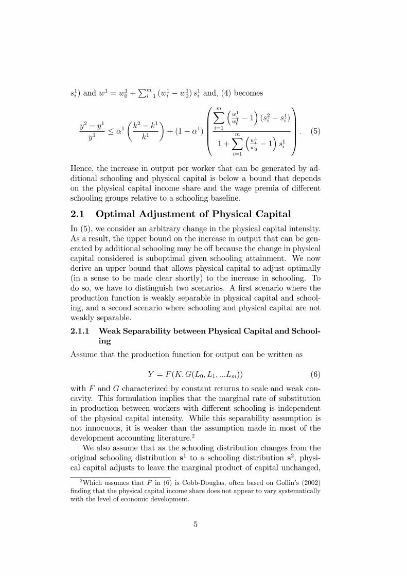
. (5)

Hence, the increase in output per worker that can be generated by ad-ditional schooling and physical capital is below a bound that dependson the physical capital income share and the wage premia of differentschooling groups relative to a schooling baseline.

2.1 Optimal Adjustment of Physical CapitalIn (5), we consider an arbitrary change in the physical capital intensity.As a result, the upper bound on the increase in output that can be gen-erated by additional schooling may be offbecause the change in physicalcapital considered is suboptimal given schooling attainment. We nowderive an upper bound that allows physical capital to adjust optimally(in a sense to be made clear shortly) to the increase in schooling. Todo so, we have to distinguish two scenarios. A first scenario where theproduction function is weakly separable in physical capital and school-ing, and a second scenario where schooling and physical capital are notweakly separable.

2.1.1 Weak Separability between Physical Capital and School-ing

Assume that the production function for output can be written as

Y = F (K,G(L0, L1, ...Lm)) (6)

with F and G characterized by constant returns to scale and weak con-cavity. This formulation implies that the marginal rate of substitutionin production between workers with different schooling is independentof the physical capital intensity. While this separability assumption isnot innocuous, it is weaker than the assumption made in most of thedevelopment accounting literature.2

We also assume that as the schooling distribution changes from theoriginal schooling distribution s1 to a schooling distribution s2, physi-cal capital adjusts to leave the marginal product of capital unchanged,

2Which assumes that F in (6) is Cobb-Douglas, often based on Gollin’s (2002)finding that the physical capital income share does not appear to vary systematicallywith the level of economic development.

5

MPK2 = MPK1. This could be because physical capital is mobile in-ternationally or because of physical capital accumulation in a closedeconomy.3 With these two assumptions we can develop an upper boundfor the increase in output per worker that can be generated by additionalschooling, that depends on the wage premia of different schooling groupsonly. To see this, note that separability of the production function im-plies

y2 − y1

y1≤ α1

(k2 − k1

k1

)+ (1− α1)

(G(s2)−G(s1)

G(s1)

). (7)

The assumption that physical capital adjusts to leave the marginal prod-uct unchanged implies that F1(k1/G(s1), 1) = F1(k

2/G(s2), 1) and there-fore k2/G(s2) = k1/G(s1). Substituting in (7),

y2 − y1

y1≤ G(s2)−G(s1)

G(s1). (8)

Weak concavity and constant returns to scale ofG imply, respectively,G(s2)−G(s1) ≤

∑mi=0Gi(s

1)(s2i − s1i ) and G(s1) =∑m

i=0Gi(s1)s1i , where

Gi denotes the derivative with respect to schooling level i. Combinedwith (7), this yields

y2 − y1

y1≤

m∑i=0

Gi(s1)(s2i − s1i )

m∑i=0

Gi(s1)s1i

=

m∑i=1

(w1iw10− 1)(s2i − s1i )

1 +m∑i=1

(w1iw10− 1)s1i

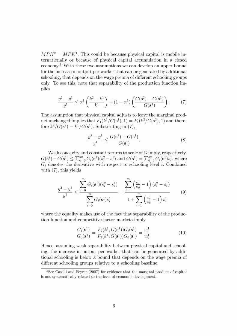
(9)

where the equality makes use of the fact that separability of the produc-tion function and competitive factor markets imply

Gi(s1)

G0(s1)=F2(k

1, G(s1))Gi(s1)

F2(k1, G(s1))G0(s1)=w1iw10. (10)

Hence, assuming weak separability between physical capital and school-ing, the increase in output per worker that can be generated by addi-tional schooling is below a bound that depends on the wage premia ofdifferent schooling groups relative to a schooling baseline.

3See Caselli and Feyrer (2007) for evidence that the marginal product of capitalis not systematically related to the level of economic development.

6

2.1.2 Non-Separability between Physical Capital and School-ing

Since Griliches (1969) and Fallon and Layard (1975), it has been ar-gued that physical capital displays stronger complementaries with high-skilled than low-skilled workers (see also Krusell et al., 2000; Caselli andColeman 2002, 2006; and Duffy et al. 2004). In this case, schoolingmay generate additional productivity gains through the complementar-ity with physical capital. We therefore extend our analysis to allowfor capital-skill complementarities and derive the corresponding upperbound for the increase in output per worker that can be generated byadditional schooling.To allow for capital-skill complementarities, suppose that the pro-

duction function is

Y = F (Q [U(L0, .., Lτ−1), H(Lτ , .., Lm)] , G [K,H(Lτ , .., Lm)]) (11)

where F,Q, U, and H are characterized by constant returns to scale andweak concavity, andG by constant returns to scale andG12 < 0 to ensurecapital-skill complementarities. This production function encompassesthe functional forms by Fallon and Layard (1975), Krusell et al.(2000),Caselli and Coleman (2002, 2006), and Goldin and Katz (1998) for exam-ple (who assume that F,G are constant-elasticity-of-substitution func-tions, that Q(U,H) = U , and that U,H are linear functions).4 The mainadvantage of our approach is that we do not need to specify functionalforms and substitution parameters, which is notoriously diffi cult (e.g.Duffy et al., 2004).To develop an upper bound for the increase in output per worker that

can be generated by increased schooling in the presence of capital-skillcomplementarities, we need an additional assumption compared to thescenario with weak separability between physical capital and schooling.The assumption is that the change in the schooling distribution from s1

to s2 does not strictly lower the skill ratio H/U , that is,

H(s22)

U(s21)≥ H(s12)

U(s11), (12)

where s1 = [s0, ..., sτ−1] collects the shares of workers with schooling lev-els strictly below τ and s2 = [sτ , ..., sm] collects the shares of workerswith schooling levels equal or higher than τ (we continue to use the su-perscript 1 to denote the original schooling shares and the superscript

4Duffy et al. (2004) argue that a special case of the formulation in (11) fits theempirical evidence better than alternative formulations for capital-skill complemen-tarities used in the literature.

7

2 for the counterfactual schooling distribution). For example, this as-sumption will be satisfied if the counterfactual schooling distributionhas lower shares of workers with schooling attainment i < τ and highershares of workers with schooling attainment i ≥ τ . If U,H are linearfunction as in Fallon and Layard (1975), Krusell et al.(2000), Caselli andColeman (2002, 2006), and Goldin and Katz (1998), the assumption in(12) is testable as it is equivalent to

τ−1∑i=0

w1iw10(s2i − s1i )

τ−1∑i=0

w1iw10s1i

≤

m∑i=τ

w1iw1τ(s2i − s1i )

m∑i=τ

w1iw1τs1i

, (13)

where we used that competitive factor markets and (11) imply w1i /w10 =

F1Q1Ui/F1Q1U0 = Ui/U0 for i < τ and w1i /w1τ = (F1Q2 + F2G2)Hi

/ (F1Q2 + F2G2)Hτ = Hi/Hτ for i ≥ τ .It can now be shown that the optimal physical capital adjustment

implies

k2 − k1

k1≤ H(s22)−H(s12)

H(s12). (14)

To see this, note that the marginal product of capital implied by (11) is

MPK = F2

1, G[

kH(s2)

, 1]

Q[U(s1)H(s2)

, 1]G1

[k

H(s2), 1

]. (15)

Hence, holding k/H constant, an increase in H/U either lowers the mar-ginal product of capital or leaves it unchanged. As a result, k/H mustfall or remain constant to leave the marginal product of physical capitalunchanged, which implies (14).Using steps that are similar to those in the derivation of (9) we obtain

U(s21)− U(s11)

U(s11)≤

τ−1∑i=0

w1iw10(s2i − s1i )

τ−1∑i=0

w1iw10s1i

, (16)

8

where we used w1i /w10 = (F1Q1Ui)/(F1Q1U0) = Hi/Hτ for i < τ, and

k2 − k1

k1≤ H(s22)−H(s12)

H(s12)≤

m∑i=τ

w1iw1τ(s2i − s1i )

m∑i=τ

w1iw1τs1i

, (17)

where we used w1i /w1τ = (F1Q2Hi + F2G2Hi) / (F1Q2Hτ + F2G2Hτ ) =

Hi/Hτ for i ≥ τ and (14). These last two inequalities combined with(11) imply

y2 − y1

y1≤ β1

τ−1∑i=0

w1iw10(s2i − s1i )

τ−1∑i=0

w1iw10s1i

+ (1− β1)

m∑i=τ

w1iw1τ(s2i − s1i )

m∑i=τ

w1iw1τs1i

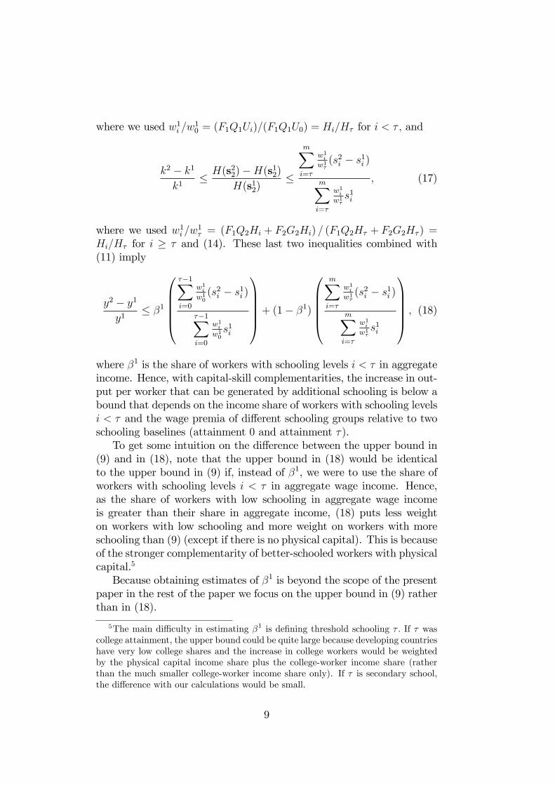
, (18)

where β1 is the share of workers with schooling levels i < τ in aggregateincome. Hence, with capital-skill complementarities, the increase in out-put per worker that can be generated by additional schooling is below abound that depends on the income share of workers with schooling levelsi < τ and the wage premia of different schooling groups relative to twoschooling baselines (attainment 0 and attainment τ).To get some intuition on the difference between the upper bound in

(9) and in (18), note that the upper bound in (18) would be identicalto the upper bound in (9) if, instead of β1, we were to use the share ofworkers with schooling levels i < τ in aggregate wage income. Hence,as the share of workers with low schooling in aggregate wage incomeis greater than their share in aggregate income, (18) puts less weighton workers with low schooling and more weight on workers with moreschooling than (9) (except if there is no physical capital). This is becauseof the stronger complementarity of better-schooled workers with physicalcapital.5

Because obtaining estimates of β1 is beyond the scope of the presentpaper in the rest of the paper we focus on the upper bound in (9) ratherthan in (18).

5The main diffi culty in estimating β1 is defining threshold schooling τ . If τ wascollege attainment, the upper bound could be quite large because developing countrieshave very low college shares and the increase in college workers would be weightedby the physical capital income share plus the college-worker income share (ratherthan the much smaller college-worker income share only). If τ is secondary school,the difference with our calculations would be small.

9

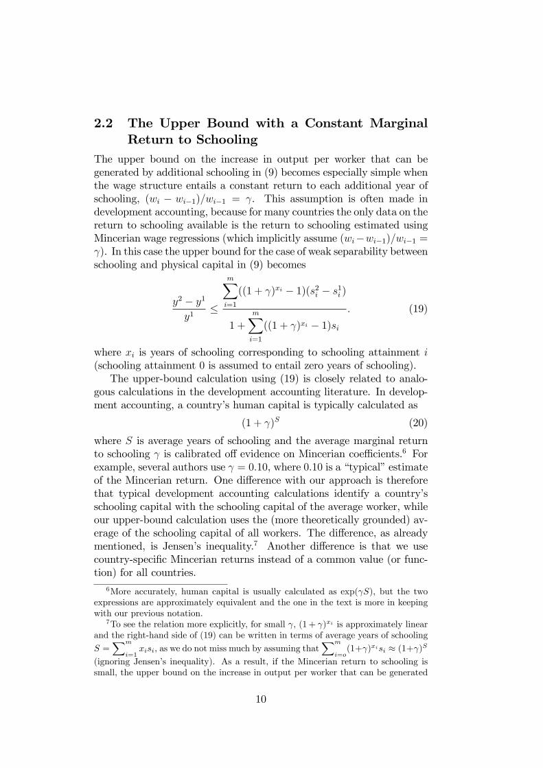
2.2 The Upper Bound with a Constant MarginalReturn to Schooling

The upper bound on the increase in output per worker that can begenerated by additional schooling in (9) becomes especially simple whenthe wage structure entails a constant return to each additional year ofschooling, (wi − wi−1)/wi−1 = γ. This assumption is often made indevelopment accounting, because for many countries the only data on thereturn to schooling available is the return to schooling estimated usingMincerian wage regressions (which implicitly assume (wi−wi−1)/wi−1 =γ). In this case the upper bound for the case of weak separability betweenschooling and physical capital in (9) becomes

y2 − y1

y1≤

m∑i=1

((1 + γ)xi − 1)(s2i − s1i )

1 +m∑i=1

((1 + γ)xi − 1)si. (19)

where xi is years of schooling corresponding to schooling attainment i(schooling attainment 0 is assumed to entail zero years of schooling).The upper-bound calculation using (19) is closely related to analo-

gous calculations in the development accounting literature. In develop-ment accounting, a country’s human capital is typically calculated as

(1 + γ)S (20)

where S is average years of schooling and the average marginal returnto schooling γ is calibrated off evidence on Mincerian coeffi cients.6 Forexample, several authors use γ = 0.10, where 0.10 is a “typical”estimateof the Mincerian return. One difference with our approach is thereforethat typical development accounting calculations identify a country’sschooling capital with the schooling capital of the average worker, whileour upper-bound calculation uses the (more theoretically grounded) av-erage of the schooling capital of all workers. The difference, as alreadymentioned, is Jensen’s inequality.7 Another difference is that we usecountry-specific Mincerian returns instead of a common value (or func-tion) for all countries.

6More accurately, human capital is usually calculated as exp(γS), but the twoexpressions are approximately equivalent and the one in the text is more in keepingwith our previous notation.

7To see the relation more explicitly, for small γ, (1 + γ)xi is approximately linearand the right-hand side of (19) can be written in terms of average years of schooling

S =∑m

i=1xisi, as we do not miss much by assuming that

∑m

i=o(1+γ)xisi ≈ (1+γ)S

(ignoring Jensen’s inequality). As a result, if the Mincerian return to schooling issmall, the upper bound on the increase in output per worker that can be generated

10

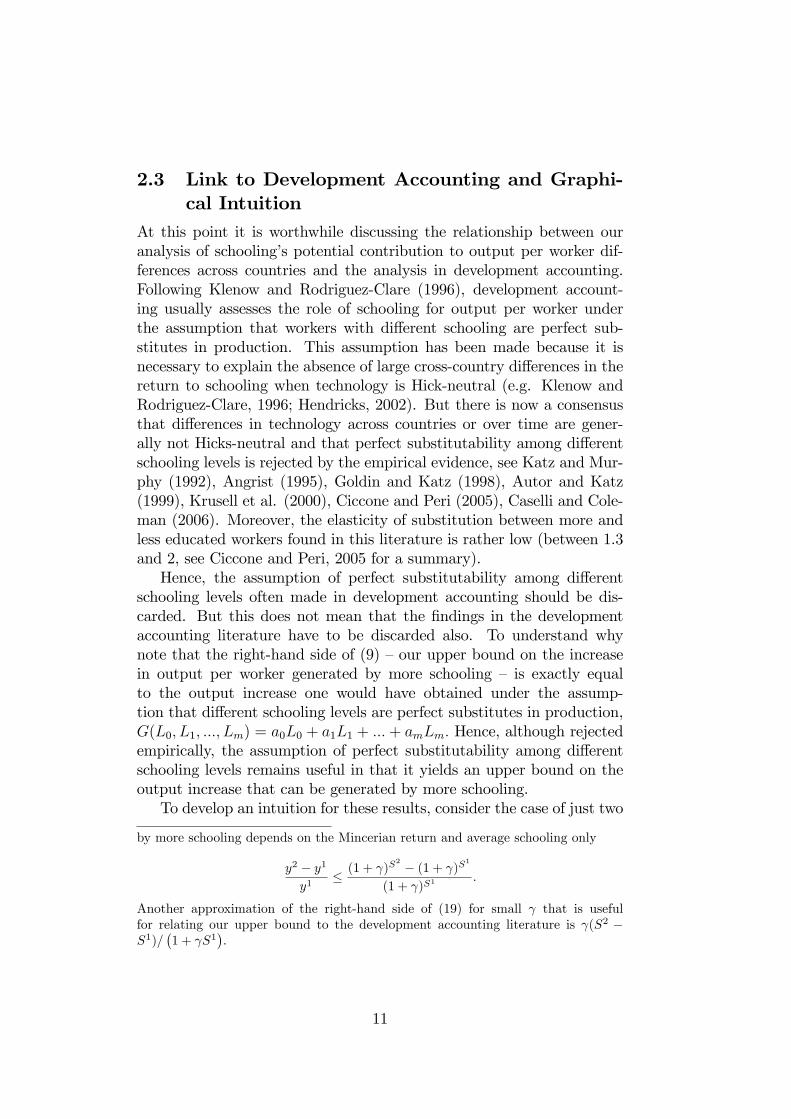
2.3 Link to Development Accounting and Graphi-cal Intuition

At this point it is worthwhile discussing the relationship between ouranalysis of schooling’s potential contribution to output per worker dif-ferences across countries and the analysis in development accounting.Following Klenow and Rodriguez-Clare (1996), development account-ing usually assesses the role of schooling for output per worker underthe assumption that workers with different schooling are perfect sub-stitutes in production. This assumption has been made because it isnecessary to explain the absence of large cross-country differences in thereturn to schooling when technology is Hick-neutral (e.g. Klenow andRodriguez-Clare, 1996; Hendricks, 2002). But there is now a consensusthat differences in technology across countries or over time are gener-ally not Hicks-neutral and that perfect substitutability among differentschooling levels is rejected by the empirical evidence, see Katz and Mur-phy (1992), Angrist (1995), Goldin and Katz (1998), Autor and Katz(1999), Krusell et al. (2000), Ciccone and Peri (2005), Caselli and Cole-man (2006). Moreover, the elasticity of substitution between more andless educated workers found in this literature is rather low (between 1.3and 2, see Ciccone and Peri, 2005 for a summary).Hence, the assumption of perfect substitutability among different

schooling levels often made in development accounting should be dis-carded. But this does not mean that the findings in the developmentaccounting literature have to be discarded also. To understand whynote that the right-hand side of (9) —our upper bound on the increasein output per worker generated by more schooling — is exactly equalto the output increase one would have obtained under the assump-tion that different schooling levels are perfect substitutes in production,G(L0, L1, ..., Lm) = a0L0 + a1L1 + ...+ amLm. Hence, although rejectedempirically, the assumption of perfect substitutability among differentschooling levels remains useful in that it yields an upper bound on theoutput increase that can be generated by more schooling.To develop an intuition for these results, consider the case of just two

by more schooling depends on the Mincerian return and average schooling only

y2 − y1y1

≤ (1 + γ)S2 − (1 + γ)S1

(1 + γ)S1.

Another approximation of the right-hand side of (19) for small γ that is usefulfor relating our upper bound to the development accounting literature is γ(S2 −S1)/

(1 + γS1

).

11

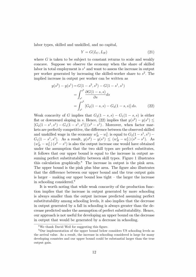
labor types, skilled and unskilled, and no capital,

Y = G(LU , LH) (21)

where G is taken to be subject to constant returns to scale and weaklyconcave. Suppose we observe the economy when the share of skilledlabor in total employment is s1 and want to assess the increase in outputper worker generated by increasing the skilled-worker share to s2. Theimplied increase in output per worker can be written as

y(s2)− y(s1)=G(1− s2, s2)−G(1− s1, s1)

=

∫ s2

s1

∂G(1− s, s)

∂sds

=

∫ s2

s1[G2(1− s, s)−G2(1− s, s)] ds. (22)

Weak concavity of G implies that G2(1 − s, s) − G1(1 − s, s) is eitherflat or downward sloping in s. Hence, (22) implies that y(s2) − y(s1) ≤[G2(1− s1, s1)−G1(1− s1, s1)] (s2 − s1) . Moreover, when factor mar-kets are perfectly competitive, the difference between the observed skilledand unskilled wage in the economy w1H −w1U is equal to G2(1− s1, s1)−G1(1 − s1, s1). As a result, y(s2) − y(s1) ≤ (w1H − w1U) (s

2 − s1). As(w1H − w1U) (s

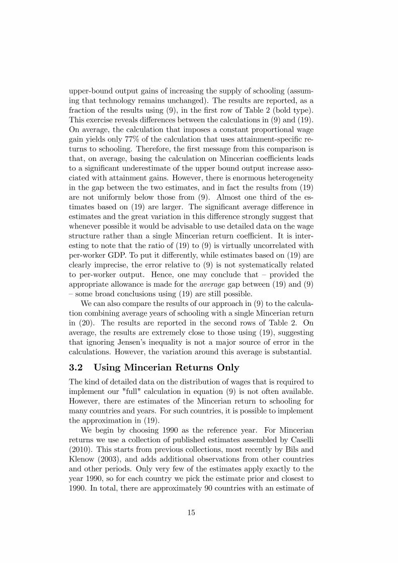
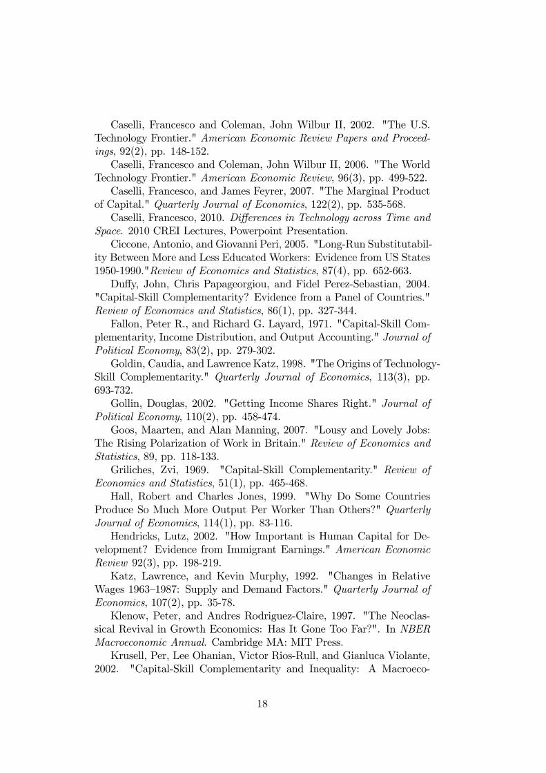
2 − s1) is also the output increase one would have obtainedunder the assumption that the two skill types are perfect substitutes,it follows that our upper bound is equal to the increase in output as-suming perfect substitutability between skill types. Figure 1 illustratesthis calculation graphically.8 The increase in output is the pink area.The upper bound is the pink plus blue area. The figure also illustratesthat the difference between our upper bound and the true output gainis larger —making our upper bound less tight —the larger the increasein schooling considered.9

It is worth noting that while weak concavity of the production func-tion implies that the increase in output generated by more schoolingis always smaller than the output increase predicted assuming perfectsubstitutability among schooling levels, it also implies that the decreasein output generated by a fall in schooling is always greater than the de-crease predicted under the assumption of perfect substitutability. Hence,our approach is not useful for developing an upper bound on the decreasein output that would be generated by a decrease in schooling.

8We thank David Weil for suggesting this figure.9Our implementation of the upper bound below considers US schooling levels as

the arrival value. As a result, the increase in schooling considered is large for manydeveloping countries and our upper bound could be substantial larger than the trueoutput gain.

12

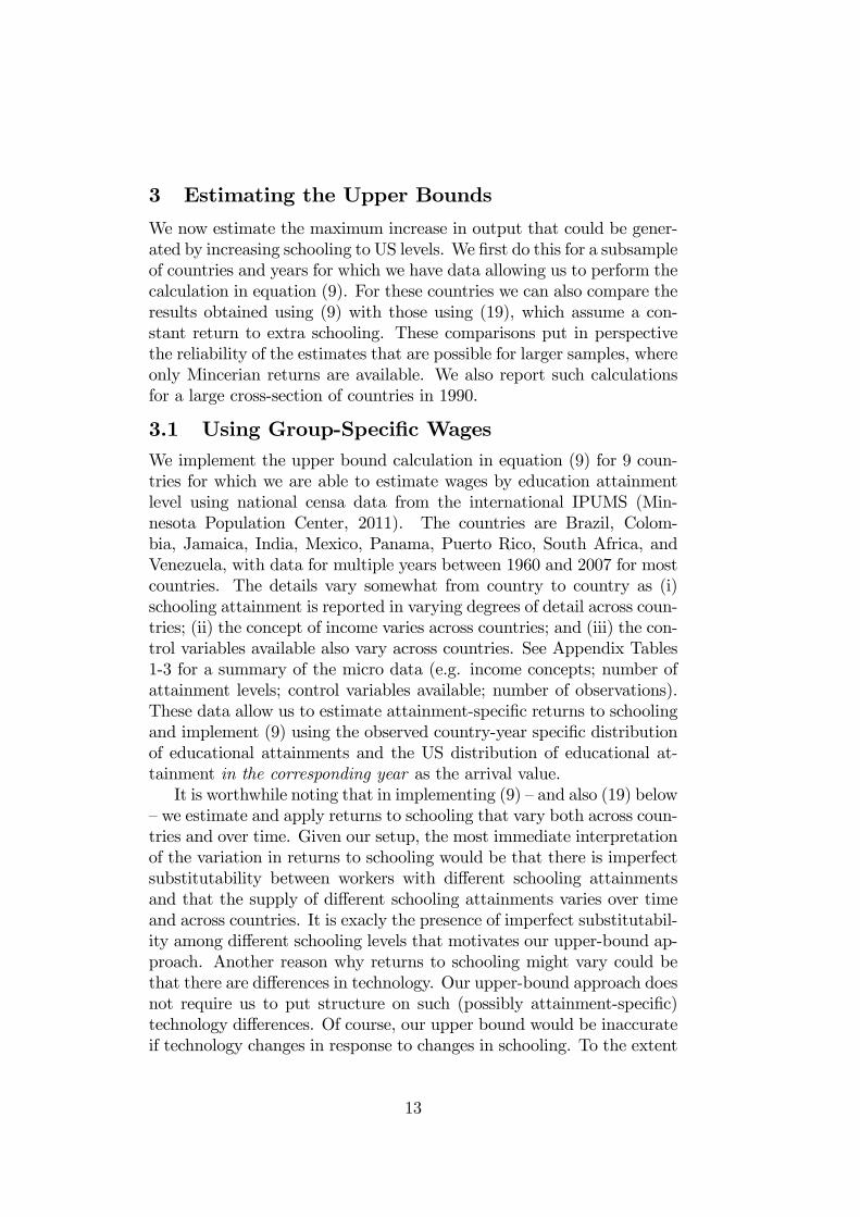
3 Estimating the Upper Bounds

We now estimate the maximum increase in output that could be gener-ated by increasing schooling to US levels. We first do this for a subsampleof countries and years for which we have data allowing us to perform thecalculation in equation (9). For these countries we can also compare theresults obtained using (9) with those using (19), which assume a con-stant return to extra schooling. These comparisons put in perspectivethe reliability of the estimates that are possible for larger samples, whereonly Mincerian returns are available. We also report such calculationsfor a large cross-section of countries in 1990.

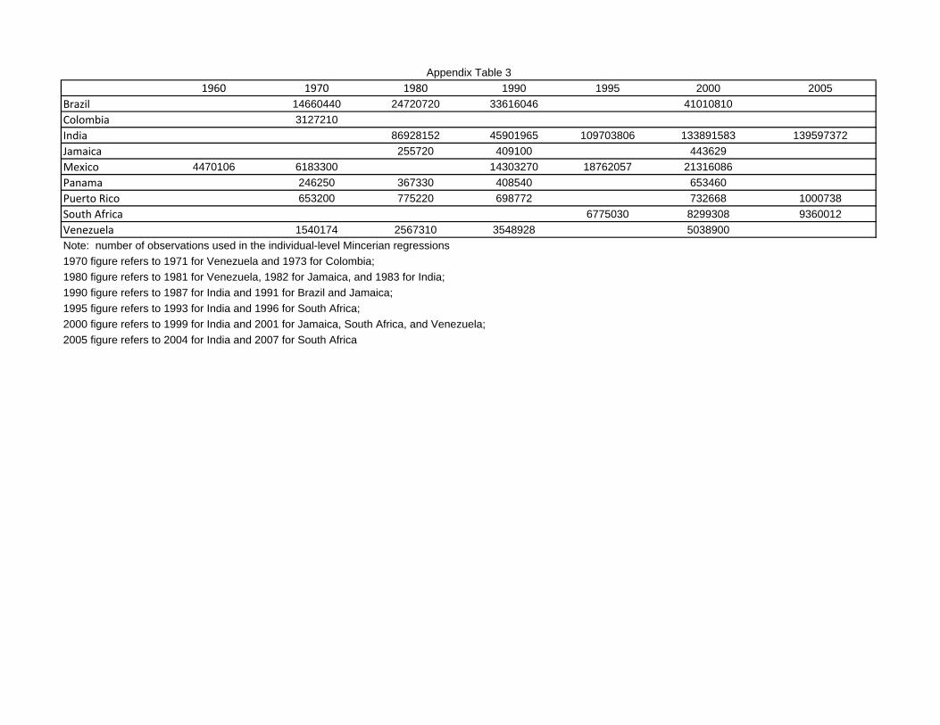
3.1 Using Group-Specific WagesWe implement the upper bound calculation in equation (9) for 9 coun-tries for which we are able to estimate wages by education attainmentlevel using national censa data from the international IPUMS (Min-nesota Population Center, 2011). The countries are Brazil, Colom-bia, Jamaica, India, Mexico, Panama, Puerto Rico, South Africa, andVenezuela, with data for multiple years between 1960 and 2007 for mostcountries. The details vary somewhat from country to country as (i)schooling attainment is reported in varying degrees of detail across coun-tries; (ii) the concept of income varies across countries; and (iii) the con-trol variables available also vary across countries. See Appendix Tables1-3 for a summary of the micro data (e.g. income concepts; number ofattainment levels; control variables available; number of observations).These data allow us to estimate attainment-specific returns to schoolingand implement (9) using the observed country-year specific distributionof educational attainments and the US distribution of educational at-tainment in the corresponding year as the arrival value.It is worthwhile noting that in implementing (9) —and also (19) below

—we estimate and apply returns to schooling that vary both across coun-tries and over time. Given our setup, the most immediate interpretationof the variation in returns to schooling would be that there is imperfectsubstitutability between workers with different schooling attainmentsand that the supply of different schooling attainments varies over timeand across countries. It is exacly the presence of imperfect substitutabil-ity among different schooling levels that motivates our upper-bound ap-proach. Another reason why returns to schooling might vary could bethat there are differences in technology. Our upper-bound approach doesnot require us to put structure on such (possibly attainment-specific)technology differences. Of course, our upper bound would be inaccurateif technology changes in response to changes in schooling. To the extent

13

that this is an objection, it applies to all the development-accountingliterature. For example, the Hall-Jones calculation would be inaccurateif total factor productivity increases in response to an increase in hu-man capital. However, our interpretation of the spirit of developmentaccounting is precisely to ask about the role of inputs holding technologyconstant.10

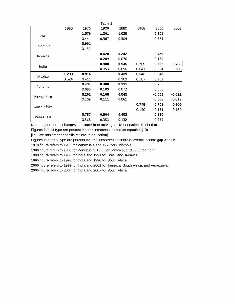
The results of implementing the upper-bound calculation in (9) foreach country-year are presented (in bold face) in Table 1. For this groupof countries applying the upper-bound calculation leads to conclusionsthat vary significantly both across countries and over time. The largestcomputed upper-bound gain is for Brazil in 1970, which is of the orderof 150%. This result largely reflects the huge gap in schooling betweenthe US and Brazil in that year (average years of schooling in Brazil wasless than 4 in 1970). The smallest upper bound is for Puerto Rico in2005, which is essentially zero, reflecting the fact that this country hadhigh education attainment by that year (average years of schooling isalmost 13). The average is 0.59.A different metric is the fraction of the overall output gap with the

US that reaching US attainment levels can cover. This calculation is alsoreported in Table 1 (characters in normal type). As a proportion of theoutput gap, the largest upper-bound gain is for Brazil in 1980 (57%),while the smallest is again for Puerto Rico in 2005 (virtually zero). Onaverage, at the upper bound attaining the US education distributionallows countries to cover 21% of their output gap with the US.The shortcoming of the results in Table 1 is that they refer to a quite

likely unrepresentative sample. For this reason, we now ask whether us-ing the approach in equation (19) leads to an acceptable approximationof (9). As we show in the next section, data to implement (19) is read-ily available for a much larger (and arguably representative) sample ofcountries, so if (19) offers an acceptable approximation to (9) we can bemore confident on results from larger samples.To implement (19), we first use our micro data to estimate Mincerian

returns for each country-year. This is done with an OLS regression usingthe same control variables employed to estimate the attainment-specificreturns to schooling above.11 See Appendix Table 2 for point estimatesand standard errors of Mincerian returns for each country-year. Oncewe have the Mincerian return we can apply equation (19) to assess the

10Another possible source of differences in schooling returns across countries issampling variation. However our estimates of both attainment specific and Mincerianreturns are extremely precise, so we think this explanation is unlikely.11The empirical labor literature finds that OLS estimates of Mincerian returns to

schooling are often close to causal estimates, see Card (1999).

14

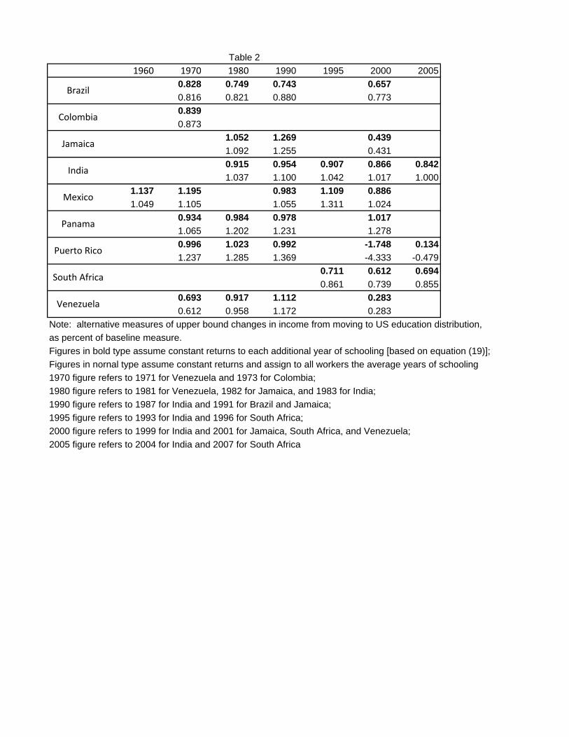
upper-bound output gains of increasing the supply of schooling (assum-ing that technology remains unchanged). The results are reported, as afraction of the results using (9), in the first row of Table 2 (bold type).This exercise reveals differences between the calculations in (9) and (19).On average, the calculation that imposes a constant proportional wagegain yields only 77% of the calculation that uses attainment-specific re-turns to schooling. Therefore, the first message from this comparison isthat, on average, basing the calculation on Mincerian coeffi cients leadsto a significant underestimate of the upper bound output increase asso-ciated with attainment gains. However, there is enormous heterogeneityin the gap between the two estimates, and in fact the results from (19)are not uniformly below those from (9). Almost one third of the es-timates based on (19) are larger. The significant average difference inestimates and the great variation in this difference strongly suggest thatwhenever possible it would be advisable to use detailed data on the wagestructure rather than a single Mincerian return coeffi cient. It is inter-esting to note that the ratio of (19) to (9) is virtually uncorrelated withper-worker GDP. To put it differently, while estimates based on (19) areclearly imprecise, the error relative to (9) is not systematically relatedto per-worker output. Hence, one may conclude that — provided theappropriate allowance is made for the average gap between (19) and (9)—some broad conclusions using (19) are still possible.We can also compare the results of our approach in (9) to the calcula-

tion combining average years of schooling with a single Mincerian returnin (20). The results are reported in the second rows of Table 2. Onaverage, the results are extremely close to those using (19), suggestingthat ignoring Jensen’s inequality is not a major source of error in thecalculations. However, the variation around this average is substantial.

3.2 Using Mincerian Returns OnlyThe kind of detailed data on the distribution of wages that is required toimplement our "full" calculation in equation (9) is not often available.However, there are estimates of the Mincerian return to schooling formany countries and years. For such countries, it is possible to implementthe approximation in (19).We begin by choosing 1990 as the reference year. For Mincerian

returns we use a collection of published estimates assembled by Caselli(2010). This starts from previous collections, most recently by Bils andKlenow (2003), and adds additional observations from other countriesand other periods. Only very few of the estimates apply exactly to theyear 1990, so for each country we pick the estimate prior and closest to1990. In total, there are approximately 90 countries with an estimate of

15

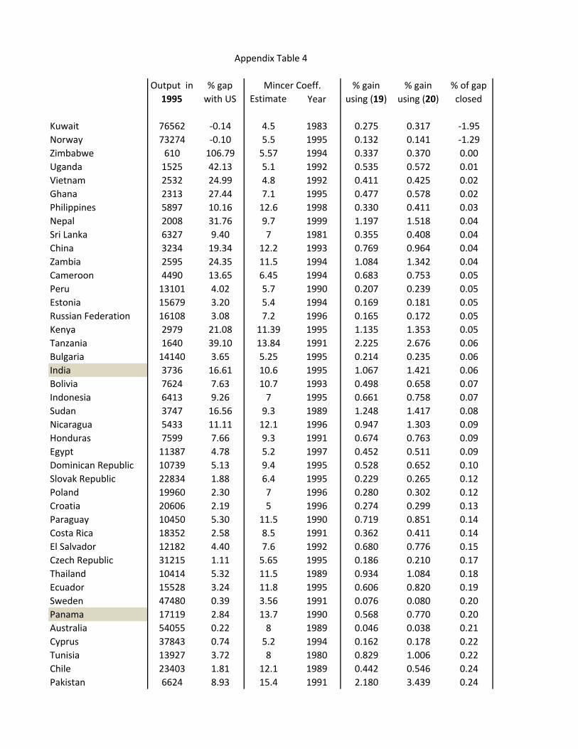
the Mincerian return prior to 1990. Country-specific Mincerian returnsand their date are shown in Appendix Table 3. For schooling attainment,we use the latest installment of the Barro and Lee data set (Barro andLee, 2010), which breaks the labor force down into 7 attainment groups,no education, some primary school, primary school completed, somesecondary school, secondary school completed, some college, and collegecompleted. These are observed in 1990 for all countries. For the referencecountry, we again take the US.12

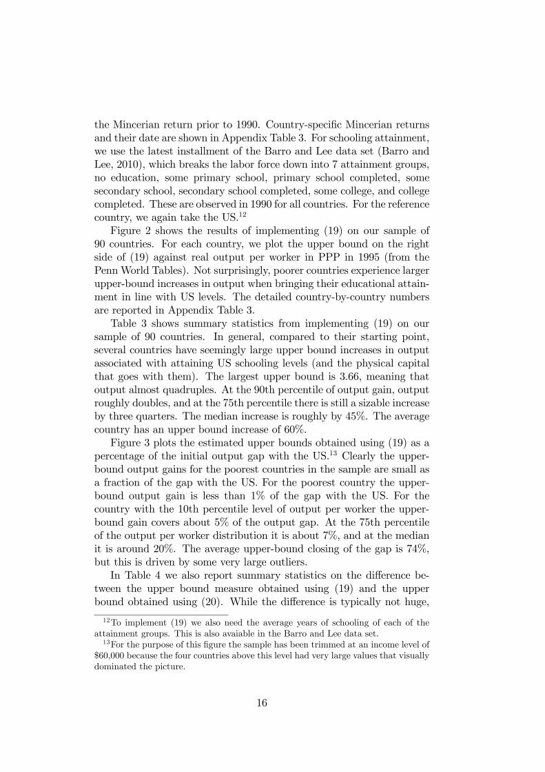
Figure 2 shows the results of implementing (19) on our sample of90 countries. For each country, we plot the upper bound on the rightside of (19) against real output per worker in PPP in 1995 (from thePennWorld Tables). Not surprisingly, poorer countries experience largerupper-bound increases in output when bringing their educational attain-ment in line with US levels. The detailed country-by-country numbersare reported in Appendix Table 3.Table 3 shows summary statistics from implementing (19) on our

sample of 90 countries. In general, compared to their starting point,several countries have seemingly large upper bound increases in outputassociated with attaining US schooling levels (and the physical capitalthat goes with them). The largest upper bound is 3.66, meaning thatoutput almost quadruples. At the 90th percentile of output gain, outputroughly doubles, and at the 75th percentile there is still a sizable increaseby three quarters. The median increase is roughly by 45%. The averagecountry has an upper bound increase of 60%.Figure 3 plots the estimated upper bounds obtained using (19) as a

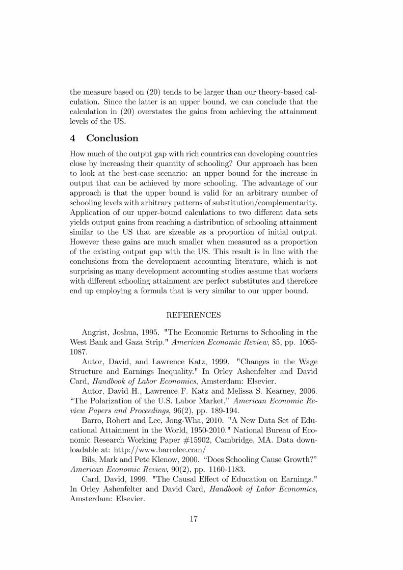
percentage of the initial output gap with the US.13 Clearly the upper-bound output gains for the poorest countries in the sample are small asa fraction of the gap with the US. For the poorest country the upper-bound output gain is less than 1% of the gap with the US. For thecountry with the 10th percentile level of output per worker the upper-bound gain covers about 5% of the output gap. At the 75th percentileof the output per worker distribution it is about 7%, and at the medianit is around 20%. The average upper-bound closing of the gap is 74%,but this is driven by some very large outliers.In Table 4 we also report summary statistics on the difference be-

tween the upper bound measure obtained using (19) and the upperbound obtained using (20). While the difference is typically not huge,

12To implement (19) we also need the average years of schooling of each of theattainment groups. This is also avaiable in the Barro and Lee data set.13For the purpose of this figure the sample has been trimmed at an income level of

$60,000 because the four countries above this level had very large values that visuallydominated the picture.

16

the measure based on (20) tends to be larger than our theory-based cal-culation. Since the latter is an upper bound, we can conclude that thecalculation in (20) overstates the gains from achieving the attainmentlevels of the US.

4 Conclusion

How much of the output gap with rich countries can developing countriesclose by increasing their quantity of schooling? Our approach has beento look at the best-case scenario: an upper bound for the increase inoutput that can be achieved by more schooling. The advantage of ourapproach is that the upper bound is valid for an arbitrary number ofschooling levels with arbitrary patterns of substitution/complementarity.Application of our upper-bound calculations to two different data setsyields output gains from reaching a distribution of schooling attainmentsimilar to the US that are sizeable as a proportion of initial output.However these gains are much smaller when measured as a proportionof the existing output gap with the US. This result is in line with theconclusions from the development accounting literature, which is notsurprising as many development accounting studies assume that workerswith different schooling attainment are perfect substitutes and thereforeend up employing a formula that is very similar to our upper bound.

REFERENCES

Angrist, Joshua, 1995. "The Economic Returns to Schooling in theWest Bank and Gaza Strip." American Economic Review, 85, pp. 1065-1087.Autor, David, and Lawrence Katz, 1999. "Changes in the Wage

Structure and Earnings Inequality." In Orley Ashenfelter and DavidCard, Handbook of Labor Economics, Amsterdam: Elsevier.Autor, David H., Lawrence F. Katz and Melissa S. Kearney, 2006.

“The Polarization of the U.S. Labor Market,”American Economic Re-view Papers and Proceedings, 96(2), pp. 189-194.Barro, Robert and Lee, Jong-Wha, 2010. "A New Data Set of Edu-

cational Attainment in the World, 1950-2010." National Bureau of Eco-nomic Research Working Paper #15902, Cambridge, MA. Data down-loadable at: http://www.barrolee.com/Bils, Mark and Pete Klenow, 2000. “Does Schooling Cause Growth?”

American Economic Review, 90(2), pp. 1160-1183.Card, David, 1999. "The Causal Effect of Education on Earnings."

In Orley Ashenfelter and David Card, Handbook of Labor Economics,Amsterdam: Elsevier.

17

Caselli, Francesco and Coleman, John Wilbur II, 2002. "The U.S.Technology Frontier." American Economic Review Papers and Proceed-ings, 92(2), pp. 148-152.Caselli, Francesco and Coleman, John Wilbur II, 2006. "The World

Technology Frontier." American Economic Review, 96(3), pp. 499-522.Caselli, Francesco, and James Feyrer, 2007. "The Marginal Product

of Capital." Quarterly Journal of Economics, 122(2), pp. 535-568.Caselli, Francesco, 2010. Differences in Technology across Time and

Space. 2010 CREI Lectures, Powerpoint Presentation.Ciccone, Antonio, and Giovanni Peri, 2005. "Long-Run Substitutabil-

ity Between More and Less Educated Workers: Evidence from US States1950-1990."Review of Economics and Statistics, 87(4), pp. 652-663.Duffy, John, Chris Papageorgiou, and Fidel Perez-Sebastian, 2004.

"Capital-Skill Complementarity? Evidence from a Panel of Countries."Review of Economics and Statistics, 86(1), pp. 327-344.Fallon, Peter R., and Richard G. Layard, 1971. "Capital-Skill Com-

plementarity, Income Distribution, and Output Accounting." Journal ofPolitical Economy, 83(2), pp. 279-302.Goldin, Caudia, and Lawrence Katz, 1998. "The Origins of Technology-

Skill Complementarity." Quarterly Journal of Economics, 113(3), pp.693-732.Gollin, Douglas, 2002. "Getting Income Shares Right." Journal of

Political Economy, 110(2), pp. 458-474.Goos, Maarten, and Alan Manning, 2007. "Lousy and Lovely Jobs:

The Rising Polarization of Work in Britain." Review of Economics andStatistics, 89, pp. 118-133.Griliches, Zvi, 1969. "Capital-Skill Complementarity." Review of

Economics and Statistics, 51(1), pp. 465-468.Hall, Robert and Charles Jones, 1999. "Why Do Some Countries

Produce So Much More Output Per Worker Than Others?" QuarterlyJournal of Economics, 114(1), pp. 83-116.Hendricks, Lutz, 2002. "How Important is Human Capital for De-

velopment? Evidence from Immigrant Earnings." American EconomicReview 92(3), pp. 198-219.Katz, Lawrence, and Kevin Murphy, 1992. "Changes in Relative

Wages 1963—1987: Supply and Demand Factors." Quarterly Journal ofEconomics, 107(2), pp. 35-78.Klenow, Peter, and Andres Rodriguez-Claire, 1997. "The Neoclas-

sical Revival in Growth Economics: Has It Gone Too Far?". In NBERMacroeconomic Annual. Cambridge MA: MIT Press.Krusell, Per, Lee Ohanian, Victor Rios-Rull, and Gianluca Violante,

2002. "Capital-Skill Complementarity and Inequality: A Macroeco-

18

nomic Analysis." Econometrica 68(4), pp. 1029-1053.McFadden, Daniel, Peter Diamond, and Miguel Rodriguez, 1978.

"Measurement of the Elasticity of Factor Substitution and the Bias ofTechnical Change." In Melvyn Fuss and Daniel McFadden, ProductionEconomics: A Dual Approach to Theory and Applications, Amsterdam:Elsevier.Minnesota Population Center. Integrated Public Use Microdata Se-

ries, International (IPUMS), 2011. Version 6.1 [Machine-Readable Data-base.]. Minneapolis: University of Minnesota. Data downloadable at:http://www.international.ipums.org

19

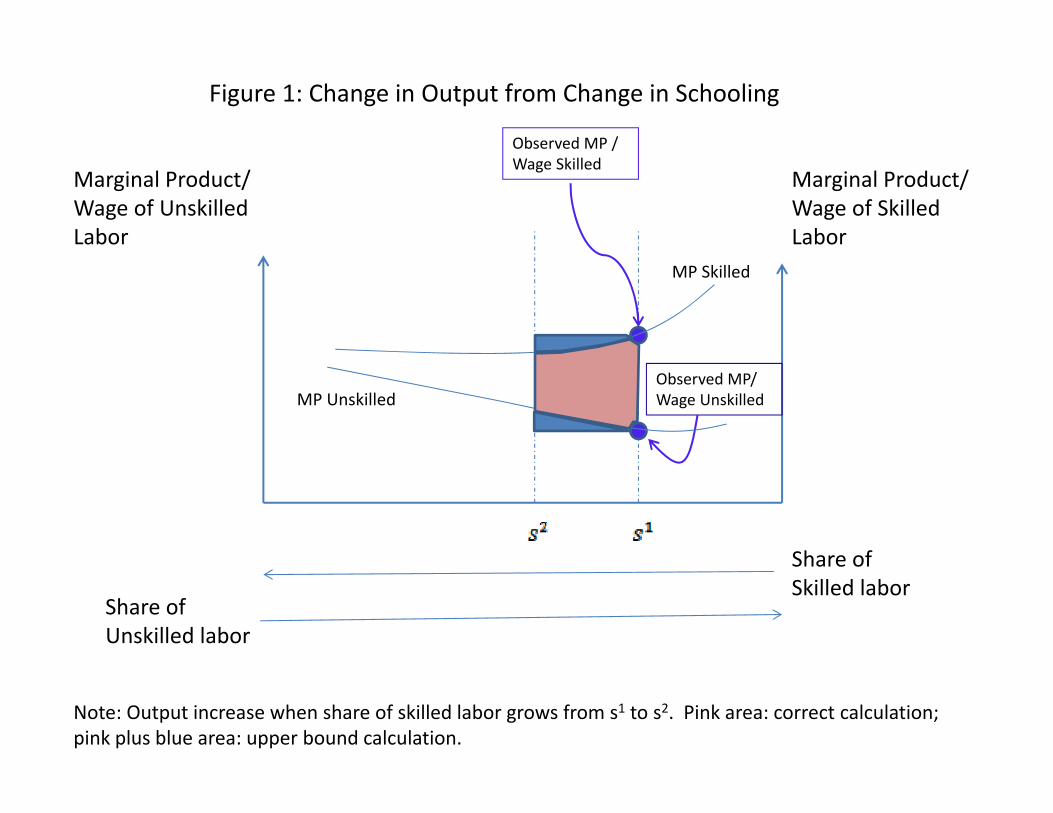
Figure 1: Change in Output from Change in Schooling

Observed MP /

Marginal Product/ Wage of Unskilled Labor

Marginal Product/ Wage of Skilled Labor

/Wage Skilled

MP Skilled

MP UnskilledObserved MP/ Wage Unskilled

Share of

Share of Unskilled labor

Share of Skilled labor 

Note: Output increase when share of skilled labor grows from s1 to s2.  Pink area: correct calculation; pink plus blue area: upper bound calculation. 

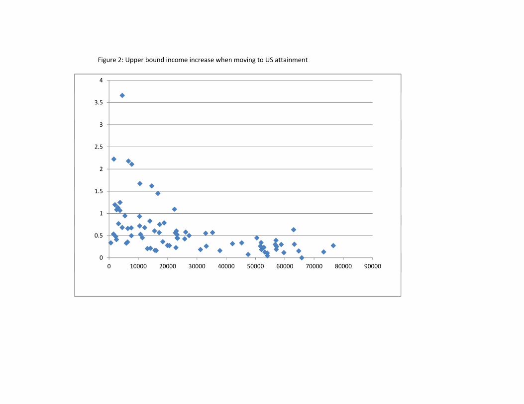
Figure 2: Upper bound income increase when moving to US attainment

4

3

3.5

4

2

2.5

3

1

1.5

2

0

0.5

1

0 10000 20000 30000 40000 50000 60000 70000 80000 900000

0 10000 20000 30000 40000 50000 60000 70000 80000 90000

Figure 3: Upper bound income gain as percent of output per worker gap with US

2

2.5

3

1

1.5

2

0

0.5

1

0 10000 20000 30000 40000 50000 60000 700000

0 10000 20000 30000 40000 50000 60000 70000

1960 1970 1980 1990 1995 2000 2005

1.576 1.201 1.020 0.901

0.441 0.567 0.304 0.2240.901

0.1590.620 0.242 0.469

0.209 0.076 0.1350.908 0.945 0.769 0.792 0.769

0.053 0.056 0.047 0.054 0.061.238 0.916 0.439 0.543 0.543

0.524 0.411 0.169 0.187 0.2010.434 0.408 0.331 0.255

0.088 0.109 0.072 0.0550.202 0.108 0.045 -0.003 -0.012

0.209 0.111 0.061 ‐0.006 ‐0.0190.745 0.708 0.609

0.140 0.129 0.1300.757 0.604 0.403 0.860

0.568 0.353 0.132 0.235Note: upper bound changes in income from moving to US education distribution.

Figures in bold type are percent income increases, based on equation (19)

[i.e. Use attainment-specific returns to education]

Figures in normal type are percent income increases as share of overall income gap with US.

1970 figure refers to 1971 for Venezuela and 1973 for Colombia;

1980 figure refers to 1981 for Venezuela, 1982 for Jamaica, and 1983 for India;

1990 figure refers to 1987 for India and 1991 for Brazil and Jamaica;

1995 figure refers to 1993 for India and 1996 for South Africa;

2000 figure refers to 1999 for India and 2001 for Jamaica, South Africa, and Venezuela;

2005 figure refers to 2004 for India and 2007 for South Africa

Puerto Rico

South Africa

Venezuela

Table 1

Brazil

Colombia

Jamaica

Mexico

Panama

India

1960 1970 1980 1990 1995 2000 2005

0.828 0.749 0.743 0.657

0.816 0.821 0.880 0.773

0.839

0.873

1.052 1.269 0.439

1.092 1.255 0.431

0.915 0.954 0.907 0.866 0.842

1.037 1.100 1.042 1.017 1.000

1.137 1.195 0.983 1.109 0.886

1.049 1.105 1.055 1.311 1.024

0.934 0.984 0.978 1.017

1.065 1.202 1.231 1.278

0.996 1.023 0.992 -1.748 0.134

1.237 1.285 1.369 -4.333 -0.479

0.711 0.612 0.694

0.861 0.739 0.855

0.693 0.917 1.112 0.283

0.612 0.958 1.172 0.283

Note: alternative measures of upper bound changes in income from moving to US education distribution,

as percent of baseline measure.

Figures in bold type assume constant returns to each additional year of schooling [based on equation (19)];

Figures in nornal type assume constant returns and assign to all workers the average years of schooling

1970 figure refers to 1971 for Venezuela and 1973 for Colombia;

1980 figure refers to 1981 for Venezuela, 1982 for Jamaica, and 1983 for India;

1990 figure refers to 1987 for India and 1991 for Brazil and Jamaica;

1995 figure refers to 1993 for India and 1996 for South Africa;

2000 figure refers to 1999 for India and 2001 for Jamaica, South Africa, and Venezuela;

2005 figure refers to 2004 for India and 2007 for South Africa

Puerto Rico

South Africa

Venezuela

Table 2

Brazil

Colombia

Jamaica

Mexico

Panama

India

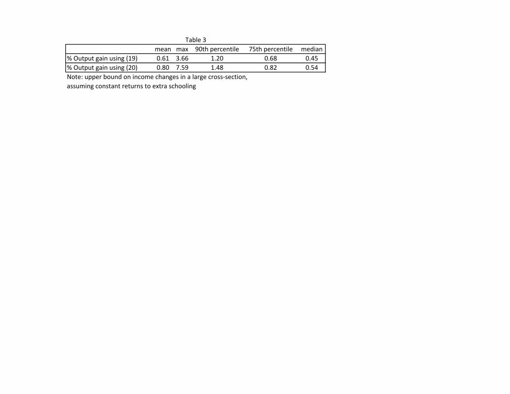
mean max 90th percentile 75th percentile median% Output gain using (19) 0.61 3.66 1.20 0.68 0.45% Output gain using (20) 0.80 7.59 1.48 0.82 0.54Note: upper bound on income changes in a large cross‐section,assuming constant returns to extra schooling

Table 3

Appendix  Table 1: Description of Individual‐Level DataIncome concept used in the analysis : total income per hour worked for 1980, 1991, 2000; total income for 1970.Other income concepts available: earned income per hour worked for 1980, 1991, 2000 (yield nearly identical results as income concept used for 1991 and 2000 but a significantly negative return to schooling in 1980).Control variables used in the analysis: age, age squared, gender, marital status, age*marital status, gender*marital status, dummies for region (state) of birth, dummies for region (state) of residence, dummy for urban area, dummy for foreign born, dummies for religion, dummies for race (except 1970).

Educational attainment levels: 8Income concept used in the analysis: total income for 1973.Other income concepts available: none.Control variables used in the analysis: age, age squared, gender, marital status, age*marital status, gender*marital status, dummies for region (state) of birth, dummies for region (municipality) of residence, dummy for urban area, dummy for foreign born.Educational attainment levels: 9

Income concept used in the analysis: wage income for 1983, 1987, 1993, 1999, 2004.Other income concepts available: none.Control variables used in the analysis: age, age squared, gender, marital status, age*marital status, gender*marital status, dummies for region (state) of residence, dummy for urban area, dummies for religion.Educational attainment levels: 8Income concept used in the analysis: wage income for 1982, 1991, 2001.Other income concepts available: none.Control variables used in the analysis: age, age squared, gender, marital status, age*marital status, gender*marital status, dummies for region (parish) of birth, dummies for region (parish) of residence, dummy for foreign born, dummies for religion, dummies for race.Educational attainment levels: 7

Income concept used in the analysis: earned income per hour worked for 1990, 1995, 2000; earned income for 1960; total income for 1970.Other income concepts available: total income per hour for 1995, 2000.Control variables used in the analysis: age, age squared, gender, marital status, age*marital status, gender*marital status, dummies for region (state) of birth, dummies for region (state) of residence, dummy for urban area, dummy for foreign born, dummies for religion (except 1995).Educational attainment levels: 10

Note: Point estimates of the Mincerian regressions and the number of observations available

are summarized in Appendix Tables 2 and 3. For more details on the variables see https://international.ipums.org/international/.

Brazil

Colombia

India

Jamaica

Mexico

Appendix  Table 1: ContinuedIncome concept used in the analysis: wage income per hour worked for 1990, 2000; wage income for 1970; total income per hour worked for 1980.Other income concepts available: earned income per hour worked for 1990, 2000; total income per hour worked for 1990 (yield nearly identical results as income concept used).Control variables used in the analysis: age, age squared, gender, marital status, age*marital status, gender*marital status, dummies for region (state) of birth (except 1990), dummies for region (district) of residence, dummy for urban area (except 1990), dummy for foreign born (except 1980).

Educational attainment levels: 8Income concept used in the analysis: wage income per hour worked for 1970, 1980, 1990, 2000, 2005.Other income concepts available: total income per hour worked for 1970, 1980, 1990, 2000, 2005; earned income per hour worked for 1990, 2000, 2005 (yield nearly identical results as income concept used.Control variables used in the analysis: age, age squared, gender, marital status, age*marital status, gender*marital status, dummies for region (metropolitan area) of residence, dummy for foreign born, dummies for race (only 2000, 2005).

Educational attainment levels: 8Income concept used in the analysis: total income per hour worked for 1996, 2007; total income for 2001.Other income concepts available: none.Control variables used in the analysis: age, age squared, gender, marital status, age*marital status, gender*marital status, dummies for region (province) of birth (except 1996), dummies for region (municipality) of residence, dummy for foreign born, dummies for religion (except 2007), dummies for race.

Educational attainment levels: 6

Income concept used in the analysis: earned income per hour worked for 1971, 1981, 2001; earned income for 1990.Other income concepts available: total income per hour worked 2001 (yields a Mincerian return to schooling of 13.7% as compared to 4.4% using earned income).Control variables used in the analysis: age, age squared, gender, marital status, age*marital status, gender*marital status, dummies for region (state) of birth, dummies for region (province) of residence, dummy for foreign born.

Educational attainment levels: 10

Note: point estimates of the Mincerian regressions and the number of observations available

are summarized in Appendix Tables 2 and 3. For more details on the variables see https://international.ipums.org/international/.

Puerto Rico

South Africa

Venezuela

Panama

1960 1970 1980 1990 1995 2000 2005

Brazil 0,124 (0,00005) 0,113 (0,00004) 0,115 (0,00004) 0,109 (0,00003)

Colombia 0,0889 (0,0005)

India 0,083 (0,00002) 0,0866 (0,00002) 0,074 (0,00002) 0,0776 (0,00001) 0,0788 (0,00001)Jamaica 0,125 (0,002) 0,0573 (0,002) 0,0614 (0,001)

Mexico 0,123 (0,0002) 0,0993 (0,0001) 0,0682 (0,0001) 0,114 (0,0001) 0,094 (0,0001)

Panama 0,0879 (0,002) 0,0911 (0,0003) 0,0941 (0,0003) 0,0916 (0,0005)

Puerto Rico 0,099 (0,0003) 0,088 (0,0005) 0,0938 (0,0005) 0,0985 (0,0005) 0,116 (0,0004)

South Africa 0,117 (0,0001) 0,11 (0,0002) 0,143 (0,0002)

Venezuela 0,0625 (0,0005) 0,0875 (0,0003) 0,0732 (0,0002) 0,0443 (0,0005)

Note: estimated Mincerian coefficients and robust standard errors in parentheses

1970 figure refers to 1971 for Venezuela and 1973 for Colombia;

1980 figure refers to 1981 for Venezuela, 1982 for Jamaica, and 1983 for India;  1990 figure refers to 1987 for India and 1991 for Brazil and Jamaica;

1995 figure refers to 1993 for India and 1996 for South Africa;

2000 figure refers to 1999 for India and 2001 for Jamaica, South Africa, and Venezuela;

2005 figure refers to 2004 for India and 2007 for South Africa

Appendix Table 2

1960 1970 1980 1990 1995 2000 2005

Brazil 14660440 24720720 33616046 41010810

Colombia 3127210

India 86928152 45901965 109703806 133891583 139597372

Jamaica 255720 409100 443629

Mexico 4470106 6183300 14303270 18762057 21316086

Panama 246250 367330 408540 653460

Puerto Rico 653200 775220 698772 732668 1000738

South Africa 6775030 8299308 9360012

Venezuela 1540174 2567310 3548928 5038900

Note: number of observations used in the individual-level Mincerian regressions

1970 figure refers to 1971 for Venezuela and 1973 for Colombia;

1980 figure refers to 1981 for Venezuela, 1982 for Jamaica, and 1983 for India;

1990 figure refers to 1987 for India and 1991 for Brazil and Jamaica;

1995 figure refers to 1993 for India and 1996 for South Africa;

2000 figure refers to 1999 for India and 2001 for Jamaica, South Africa, and Venezuela;

2005 figure refers to 2004 for India and 2007 for South Africa

Appendix Table 3

Estimate Year

Kuwait 76562 ‐0.14 4.5 1983 0.275 0.317 ‐1.95Norway 73274 ‐0.10 5.5 1995 0.132 0.141 ‐1.29Zimbabwe 610 106.79 5.57 1994 0.337 0.370 0.00Uganda 1525 42.13 5.1 1992 0.535 0.572 0.01Vietnam 2532 24.99 4.8 1992 0.411 0.425 0.02Ghana 2313 27.44 7.1 1995 0.477 0.578 0.02Philippines 5897 10.16 12.6 1998 0.330 0.411 0.03Nepal 2008 31.76 9.7 1999 1.197 1.518 0.04Sri Lanka 6327 9.40 7 1981 0.355 0.408 0.04China 3234 19.34 12.2 1993 0.769 0.964 0.04Zambia 2595 24.35 11.5 1994 1.084 1.342 0.04Cameroon 4490 13.65 6.45 1994 0.683 0.753 0.05Peru 13101 4.02 5.7 1990 0.207 0.239 0.05Estonia 15679 3.20 5.4 1994 0.169 0.181 0.05Russian Federation 16108 3.08 7.2 1996 0.165 0.172 0.05Kenya 2979 21.08 11.39 1995 1.135 1.353 0.05Tanzania 1640 39.10 13.84 1991 2.225 2.676 0.06Bulgaria 14140 3.65 5.25 1995 0.214 0.235 0.06India 3736 16.61 10.6 1995 1.067 1.421 0.06Bolivia 7624 7.63 10.7 1993 0.498 0.658 0.07Indonesia 6413 9.26 7 1995 0.661 0.758 0.07Sudan 3747 16.56 9.3 1989 1.248 1.417 0.08Nicaragua 5433 11.11 12.1 1996 0.947 1.303 0.09Honduras 7599 7.66 9.3 1991 0.674 0.763 0.09Egypt 11387 4.78 5.2 1997 0.452 0.511 0.09Dominican Republic 10739 5.13 9.4 1995 0.528 0.652 0.10Slovak Republic 22834 1.88 6.4 1995 0.229 0.265 0.12Poland 19960 2.30 7 1996 0.280 0.302 0.12Croatia 20606 2.19 5 1996 0.274 0.299 0.13Paraguay 10450 5.30 11.5 1990 0.719 0.851 0.14Costa Rica 18352 2.58 8.5 1991 0.362 0.411 0.14El Salvador 12182 4.40 7.6 1992 0.680 0.776 0.15Czech Republic 31215 1.11 5.65 1995 0.186 0.210 0.17Thailand 10414 5.32 11.5 1989 0.934 1.084 0.18Ecuador 15528 3.24 11.8 1995 0.606 0.820 0.19Sweden 47480 0.39 3.56 1991 0.076 0.080 0.20Panama 17119 2.84 13.7 1990 0.568 0.770 0.20Australia 54055 0.22 8 1989 0.046 0.038 0.21Cyprus 37843 0.74 5.2 1994 0.162 0.178 0.22Tunisia 13927 3.72 8 1980 0.829 1.006 0.22Chile 23403 1.81 12.1 1989 0.442 0.546 0.24Pakistan 6624 8.93 15.4 1991 2.180 3.439 0.24

Appendix Table 4

Output  in 1995

% gap with US

Mincer Coeff. % gain using (19)

% gain using (20)

% of gap closed

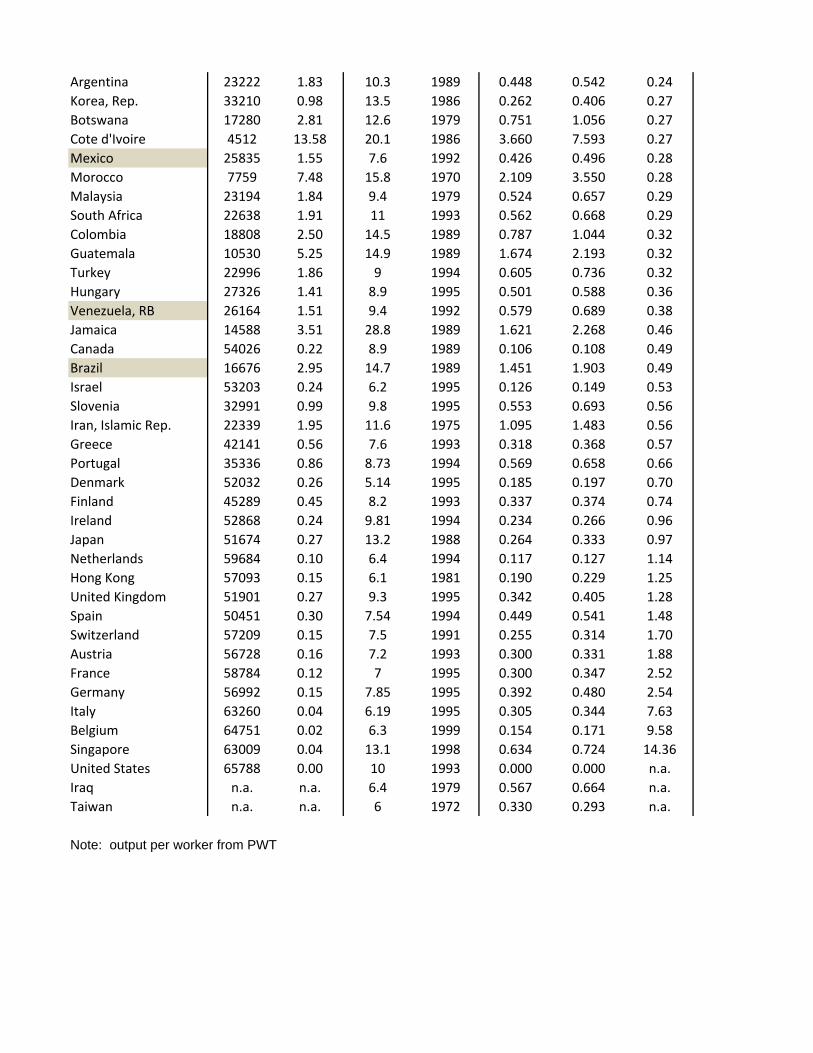
Argentina 23222 1.83 10.3 1989 0.448 0.542 0.24Korea, Rep. 33210 0.98 13.5 1986 0.262 0.406 0.27Botswana 17280 2.81 12.6 1979 0.751 1.056 0.27Cote d'Ivoire 4512 13.58 20.1 1986 3.660 7.593 0.27Mexico 25835 1.55 7.6 1992 0.426 0.496 0.28Morocco 7759 7.48 15.8 1970 2.109 3.550 0.28Malaysia 23194 1.84 9.4 1979 0.524 0.657 0.29South Africa 22638 1.91 11 1993 0.562 0.668 0.29Colombia 18808 2.50 14.5 1989 0.787 1.044 0.32Guatemala 10530 5.25 14.9 1989 1.674 2.193 0.32Turkey 22996 1.86 9 1994 0.605 0.736 0.32Hungary 27326 1.41 8.9 1995 0.501 0.588 0.36Venezuela, RB 26164 1.51 9.4 1992 0.579 0.689 0.38Jamaica 14588 3.51 28.8 1989 1.621 2.268 0.46Canada 54026 0.22 8.9 1989 0.106 0.108 0.49Brazil 16676 2.95 14.7 1989 1.451 1.903 0.49Israel 53203 0.24 6.2 1995 0.126 0.149 0.53Slovenia 32991 0.99 9.8 1995 0.553 0.693 0.56Iran, Islamic Rep. 22339 1.95 11.6 1975 1.095 1.483 0.56Greece 42141 0.56 7.6 1993 0.318 0.368 0.57Portugal 35336 0.86 8.73 1994 0.569 0.658 0.66Denmark 52032 0.26 5.14 1995 0.185 0.197 0.70Finland 45289 0.45 8.2 1993 0.337 0.374 0.74Ireland 52868 0.24 9.81 1994 0.234 0.266 0.96Japan 51674 0.27 13.2 1988 0.264 0.333 0.97Netherlands 59684 0.10 6.4 1994 0.117 0.127 1.14Hong Kong 57093 0.15 6.1 1981 0.190 0.229 1.25United Kingdom 51901 0.27 9.3 1995 0.342 0.405 1.28Spain 50451 0.30 7.54 1994 0.449 0.541 1.48Switzerland 57209 0.15 7.5 1991 0.255 0.314 1.70Austria 56728 0.16 7.2 1993 0.300 0.331 1.88France 58784 0.12 7 1995 0.300 0.347 2.52Germany 56992 0.15 7.85 1995 0.392 0.480 2.54Italy 63260 0.04 6.19 1995 0.305 0.344 7.63Belgium 64751 0.02 6.3 1999 0.154 0.171 9.58Singapore 63009 0.04 13.1 1998 0.634 0.724 14.36United States 65788 0.00 10 1993 0.000 0.000 n.a.Iraq n.a. n.a. 6.4 1979 0.567 0.664 n.a.Taiwan n.a. n.a. 6 1972 0.330 0.293 n.a.

Note: output per worker from PWT

CENTRE FOR ECONOMIC PERFORMANCE

Recent Discussion Papers

1101 Alan Manning

Barbara Petrongolo

How Local Are Labour Markets? Evidence

from a Spatial Job Search Model

1100 Fabrice Defever

Benedikt Heid

Mario Larch

Spatial Exporters

1099 John T. Addison

Alex Bryson

André Pahnke

Paulino Teixeira

Change and Persistence in the German Model

of Collective Bargaining and Worker

Representation

1098 Joan Costa-Font

Mireia Jofre-Bonet

Anorexia, Body Image and Peer Effects:

Evidence from a Sample of European Women

1097 Michal White

Alex Bryson

HRM and Workplace Motivation:

Incremental and Threshold Effects

1096 Dominique Goux

Eric Maurin

Barbara Petrongolo

Worktime Regulations and Spousal Labor

Supply

1095 Petri Böckerman

Alex Bryson

Pekka Ilmakunnas

Does High Involvement Management

Improve Worker Wellbeing?

1094 Olivier Marie

Judit Vall Castello

Measuring the (Income) Effect of Disability

Insurance Generosity on Labour Market

Participation

1093 Claudia Olivetti

Barbara Petrongolo

Gender Gaps Across Countries and Skills:

Supply, Demand and the Industry Structure

1092 Guy Mayraz Wishful Thinking

1091 Francesco Caselli

Andrea Tesei

Resource Windfalls, Political Regimes, and

Political Stability

1090 Keyu Jin

Nan Li

Factor Proportions and International Business

Cycles

1089 Yu-Hsiang Lei

Guy Michaels

Do Giant Oilfield Discoveries Fuel Internal

Armed Conflicts?

1088 Brian Bell

John Van Reenen

Firm Performance and Wages: Evidence from

Across the Corporate Hierarchy

1087 Amparo Castelló-Climent

Ana Hidalgo-Cabrillana

The Role of Educational Quality and Quantity

in the Process of Economic Development

1086 Amparo Castelló-Climent

Abhiroop Mukhopadhyay

Mass Education or a Minority Well Educated

Elite in the Process of Development: the Case

of India

1085 Holger Breinlich Heterogeneous Firm-Level Responses to

Trade Liberalisation: A Test Using Stock

Price Reactions

1084 Andrew B. Bernard

J. Bradford Jensen

Stephen J. Redding

Peter K. Schott

The Empirics of Firm Heterogeneity and

International Trade

1083 Elisa Faraglia

Albert Marcet

Andrew Scott

In Search of a Theory of Debt Management

1082 Holger Breinlich

Alejandro Cuñat

A Many-Country Model of Industrialization

1081 Francesca Cornaglia

Naomi E. Feldman

Productivity, Wages and Marriage: The Case

of Major League Baseball

1080 Nicholas Oulton The Wealth and Poverty of Nations: True

PPPs for 141 Countries

1079 Gary S. Becker

Yona Rubinstein

Fear and the Response to Terrorism: An

Economic Analysis

1078 Camille Landais

Pascal Michaillat

Emmanuel Saez

Optimal Unemployment Insurance over the

Business Cycle

1077 Klaus Adam

Albert Marcet

Juan Pablo Nicolini

Stock Market Volatility and Learning

1076 Zsófia L. Bárány The Minimum Wage and Inequality - The

Effects of Education and Technology

1075 Joanne Lindley

Stephen Machin

Rising Wage Inequality and Postgraduate

Education

1074 Stephen Hansen

Michael McMahon

First Impressions Matter: Signalling as a

Source of Policy Dynamics

1073 Ferdinand Rauch Advertising Expenditure and Consumer

Prices

The Centre for Economic Performance Publications Unit

Tel 020 7955 7673 Fax 020 7955 7595

Email info@cep.lse.ac.uk Web site http://cep.lse.ac.uk