ISSN 2042-2695

CEP Discussion Paper No 1047

March 2011

(updated December 2011)

Priors and Desires

Guy Mayraz

Abstract This paper offers a simple but powerful model of wishful thinking, cognitive dissonance, and

related biases. Choices maximize subjective expected utility, but beliefs depend on the

decision maker's interests as well as on relevant information. Simplifying assumptions yield a

representation in which the payoff in an event affects beliefs as if it were part of the evidence

about its likelihood. A single parameter determines both the direction and weight of this

`evidence', with positive values corresponding to optimism and negative values to pessimism.

Changes to a person's interests amount to new `evidence', and can alter beliefs even in the

absence of new information. The magnitude of the bias increases with the degree of

uncertainty and the strength of the decision maker's interests. High stakes can reduce the bias

indirectly by increasing incentives to acquire information, but are otherwise consistent with

substantial bias. Exploring applications, I show that wishful thinking can lead investors to

become progressively more exposed to risk, and that while improved policing unambiguously

deters crime, increased punishment may have little or no deterrent value.

JEL Classifications: D01, D03, D80, D81, D83, D84

Keywords: wishful thinking, cognitive dissonance, reference-dependent beliefs, reference-

dependent preferences

This paper was produced as part of the Centre’s Wellbeing Programme. The Centre for

Economic Performance is financed by the Economic and Social Research Council.

Acknowledgements I am grateful to Vincent Crawford, Peter Klibano , Sujoy Mukerji, Wolfgang Pesendorfer,

Matthew Rabin, Peyton Young, and particularly to Erik Eyster for stimulating discussions

and advice. I am also thankful to seminar and conference participants at Bar-Ilan, Ben-

Gurion, Berkeley, CalTech, Collegio Carlo Alberto, Edinburgh, Essex, Hebrew University,

LSE, Maastricht, MIT, Oxford, Royal Holloway, Tel- Aviv, UBC, UCL, UCSB, Warwick,

Gerzensee, RUD, and SITE.

Guy Mayraz is a Research Officer with the Wellbeing Programme at the Centre for

Economic Performance, London School of Economics. He is also a Postdoctoral Research

Fellow with the Department of Economics and Nuffield College, Oxford.

Published by

Centre for Economic Performance

London School of Economics and Political Science

Houghton Street

London WC2A 2AE

All rights reserved. No part of this publication may be reproduced, stored in a retrieval

system or transmitted in any form or by any means without the prior permission in writing of

the publisher nor be issued to the public or circulated in any form other than that in which it

is published.

Requests for permission to reproduce any article or part of the Working Paper should be sent

to the editor at the above address.

G. Mayraz, submitted 2011

1 Introduction

Beliefs depend not only on what people know to be true, but also on what they

want to be true. This paper introduces a model of decision making that allows for

this possibility, and uses a number of simplifying assumptions to obtain a tractable

and generally applicable representation. The model provides a unified account of

wishful thinking, overoptimism, overconfidence, cognitive dissonance, and unrealistic

pessimism, and can be used to study their implications for decision making. The

psychology evidence for these biases spans decades. The economics evidence is much

less extensive, but includes a wide variety of situations.1 Theoretical applications

extend into additional areas.2

This paper is hardly the first to offer a model of these biases, but it differs markedly

from the previous literature. The common approach is to model biased beliefs as an

optimal delusion: decision makers start the planning horizon with unbiased beliefs,

and choose a distorted prior so as to maximize their total discounted utility, including

utility from anticipation (Akerlof and Dickens, 1982; Brunnermeier and Parker, 2005).3

Optimal delusion models can plausibly explain many cases of optimistic bias. For

example, a moderate bias over health risks can be seen as a trade-off between the desire

to minimize fear and the possibility that biased beliefs would result in behavior that

would make disease more likely. A moderate level of bias is, however, predicated on

relevant choices having correspondingly moderate stakes. In the limit of low stakes the

bias is extreme, and in the limit of high stakes it disappears entirely. By assumption, it

is not possible to model situations in which the bias leads to welfare loss in expectation.

Optimism in such models is related to risk and ambiguity preferences. Since riskier

1 Babcock and Loewenstein (1997) find that parties in negotiations are affected by wishful thinking,resulting in an inefficient failure to reach agreement. Camerer and Lovallo (1999) link excess entryinto competitive markets to overconfidence over relative ability. Malmendier and Tate (2008) arguethat managerial overconfidence is responsible for corporate investment distortions. Cowgill et al.(2009) find optimistic bias in corporate prediction markets. Mullainathan and Washington (2009)find that voting for a candidate results in more positive views about the candidate. Park and Santos-Pinto (2010) provide field evidence for overconfidence in tournaments. Mayraz (2011) finds that aperson’s expectations for the future price of a financial asset depend on whether he or she gains fromhigh or low prices. Hoffman (2011a,b) finds that truck drivers are optimistically biased about theirproductivity (and hence their pay), resulting in an inefficient failure to switch jobs.

2For example, credit markets (De Meza and Southey, 1996), banking (Manove and Padilla, 1999),corporate finance (Heaton, 2002), search (Dubra, 2004), savings (Brunnermeier and Parker, 2005),insurance (Sandroni and Squintani, 2007), price discrimination (Eliaz and Spiegler, 2008), incentivesin organizations (Santos-Pinto, 2008), and financial contracting (Landier and Thesmar, 2009). Studiesof overconfidence over the accuracy of signals are excluded from this list.

2

bets offer more scope for bias, optimism implies a ceteris paribus preference for risk.

If optimism is restricted to beliefs over ambiguous bets, it further implies a ceteris

paribus preference for ambiguity.4

This paper’s approach is very different. Decision makers take their beliefs as given,

and maximize subjective expected utility in their choices. Their beliefs may, however,

depend on what they want to be true prior to making their choice. A number of

simplifying assumptions are imposed, yielding a representation with one non-standard

parameter, which determines both the direction and magnitude of the bias.

Some predictions are broadly similar to those of optimal delusion models. For

example, optimists underestimate their health risks, much as they would in an optimal

delusion model. The degree of bias is, however, independent of the impact on future

choices, and a substantial bias may occur even if its cost is high. Decision makers

are only biased about a choice if its outcome hangs on events that form part of their

existing interests. There is thus no general tendency to favor risky or ambiguous bets.

On the other hand, choices that align (conflict) with an optimist’s existing interests

are perceived to be relatively likely (unlikely) to lead to desirable outcomes. This

feature of the model leads to path dependence: an optimist who is invested in some

asset is biased in favor of increasing her exposure to the asset and against replacing

her existing investment with an opposite bet.5

Changes to the decision maker’s interests affect beliefs, even if the relevant in-

formation is unchanged. This makes it possible to model cognitive dissonance as a

dynamic version of wishful thinking. For example, Knox and Inkster (1968) find that

when bettors commit to place a bet on a horse, their confidence that the horse would

win the race goes up. This finding can be readily explained by the change in interests:

the bettors are initially indifferent as to which horse would win the race, but once they

place the bet they gain an interest in ‘their’ horse winning. Beliefs are thus initially

unbiased, but become biased once the bet is placed. Exogenous changes in interests

are also predicted to affect beliefs. For example, the finding that congressmen become

more positive about women’s interests after fathering a daughter (Washington, 2008)

3There are a number of papers in which agents manipulate their belief indirectly, by strategicallychoosing what information to consume (Carrillo and Mariotti, 2000; Koszegi, 2006) or by a biasedmemory process (Benabou and Tirole, 2002; Compte and Postlewaite, 2004; Gottlieb, 2010).

4The connection between optimism (or pessimism) and preferences for risk and ambiguity is alsoshared by such models as Hey (1984), Bracha and Brown (2010) and Dillenberger et al. (2011), inwhich the probabilities used to evaluate an alternative vary with the payoffs in that alternative.

5In a labor context, such path dependence would lead to an inefficiently low rate of quitting,consistent with the findings in Hoffman (2011a,b).

3

can be explained by the consequent increase in alignment between a congressman’s

interests and those of women.6

The core of the model is the precise relationship between a decision maker’s beliefs

and her interests. Subjective beliefs are represented by a probability measure over the

set of states, and interests are represented by a payoff-function, or the mapping associ-

ating each state with the utility that the decision maker obtains in that state. Letting

f denote the payoff-function, I let π f denote the resulting probability measure. In

order to obtain a tractable representation, I make a number of simplifying assump-

tions, which take the form of special circumstances in which different payoff-functions

do not result in different beliefs.

The formal framework and simplifying assumptions are presented in Section 2. A

representation theorem establishes that the assumptions are necessary and sufficient

conditions for the existence of a probability measure p and a real-valued parameter

ψ , such that for any payoff-function f and any event A,

π f (A) ∝∫

Aeψ f dp. (1)

Equation 1 takes a simpler form if the state-space is discrete, when it can be written

as follows, where s is any state:

π f (s) ∝ p(s)eψ f (s). (2)

To understand this representation note first that if f is constant then π f = p. The

probability measure p therefore represents the decision maker’s indifference beliefs,

or the beliefs she would hold if she were a completely disinterested observer who is

indifferent between all states. More generally, f is not constant, and π f depends on

both f and on ψ . If ψ is positive (negative) π f is higher in states in which payoff

is higher (lower). A positive value of ψ therefore represents optimistic bias, and a

negative value represents pessimistic bias. The larger ψ is in absolute terms, the

greater the bias. In analogy with relative risk-aversion, ψ can be thought of as the

coefficient of relative optimism. Standard decision makers are represented by ψ = 0.

Such decision makers are realists, and for them π f = p for all f .

Section 3 completes the model, and provides it with a revealed preferences axiom-

atization. The overall framework is that of reference-dependent preferences, where

6Socialization is an alternative explanation (Washington, 2008).

4

preferences are over alternatives (acts), and the reference corresponds to the map-

ping from states to consequences that characterizes the decision maker prior to the

new choice. Axioms ensure (i) that holding the reference constant, preferences have a

subjective expected utility representation, (ii) that the utility function is not reference-

dependent (making this a model of reference-dependent beliefs), (iii) that the reference

affects beliefs only via the interests that follows from it, and (iv) that beliefs relate to

interests via Equation 1.

In the representation that follows from the axioms, each decision maker is defined

by a utility function u, a probability measure p, and a coefficient of relative optimism

ψ .7 Let f denote the payoff-function representing the decision maker’s interests before

being presented with the choice set. According to the model, her choice maximizes

the expectation of u given π f , where π f is given by Equation 1.

One interpretation of the model is that subjective judgment is in some people

biased in an optimistic directions, and in others in a pessimistic direction. Decision

makers have standard tastes, and seek to maximize their (true) expected utility. Fre-

quently, however, they find themselves having to resort to subjective judgment when

assessing the likelihood of events,8 and in those cases they end up with biased beliefs.

Biased beliefs then lead to biased choices.

The model with ψ > 0 provides a unified account of wishful thinking and cognitive

dissonance. These two biases can be seen, respectively, as simply the cross-sectional

and time-series manifestations of optimism. Overoptimism and overconfidence in abil-

ity can be viewed as special cases of wishful-thinking.9 The model with ψ < 0 can be

used to represent unrealistic pessimism (Seligman, 1998).

Section 4 takes a closer look at the equations relating beliefs to interests. An

important insight is that they are formally identical to Bayes Rule, with p standing

for prior beliefs, π f for posterior beliefs, and ψ f (s) for the log likelihood in state s.

It is thus as if optimists (pessimists) are Bayesian belief updaters, who believe that

7ψ and u are identified together, and the representation is unique up to a positive affine transfor-mation. If u is replaced by u′ = au + b, ψ must be replaced by ψ ′ = ψ/a.

8Knight (1921) emphasized the importance of subjective judgment in decisions under uncertainty:“Business decisions, for example, deal with situations which are far too unique, generally speaking,for any sort of statistical tabulation to have any value for guidance. The conception of an objectivelymeasurable probability or chance is simply inapplicable.” (III.VII.47); “Yet it is true, and the fact canhardly be overemphasized, that a judgment of probability is actually made in such cases.” (III.VII.40).

9Overoptimism is exemplified by the Weinstein (1980) finding that students believe desirable(undesirable) life events are more (less) likely to happen to them than to other students. TheSvenson (1981) finding that most people believe themselves to be better drivers than most otherpeople is the best known example of overconfidence.

5

Nature has chosen the state of the world so as to make life better (worse) for them.

The comparative statics of the model are that the bias is increasing in the degree of

optimism or pessimism, the strength of the decision maker’s interests, and the degree

of subjective uncertainty.10 High-stakes decisions result in smaller bias only if the

increased incentive to invest in information reduces the decision maker’s uncertainty.

If good information is not available, a substantial bias may remain in spite of its costly

consequences.11

Section 5 examines belief updating. Changes to the decision maker’s interests

can alter beliefs even in the absence of new information, as in the Knox and Inkster

(1968) study of horse bettors. A more subtle phenomenon appears whenever the

decision maker’s interests involve a non-linear function of events. News about one

event can then alter the subjective probability of the other, even if the two events are

independent. For example, a professor’s belief about the importance of publishing in

a top journal may depend on whether her paper is accepted.

When using the model in a new application it is necessary to introduce modeling

assumptions for p and for ψ . One option is to reinterpret rational expectations as

applying to the indifference beliefs p. Optimistic bias can be modeled simply by

assuming that ψ is positive. Consider the beliefs of investors during an asset bubble.

The implication of rational expectations is that investors with no exposure to the

asset hold unbiased beliefs about the prospect of market collapse. The assumption

that ψ > 0 implies that investors who hold the asset underestimate this probability.

The model makes it possible to adapt existing applications to incorporate the

implications of wishful thinking and cognitive dissonance. Suppose an agent in some

model maximizes expected utility given beliefs p and utility function u. In adapting

the model to allow for wishful thinking, the natural assumption is that p represents

the agent’s indifference beliefs. Equation 1 can be used to compute the distorted

probability measure π f , which can then be used in place of p in predicting the agent’s

choices.

Section 6 presents two applications. The first shows that an optimism leads in-

vestors to escalate risky investments. The intuition is that taking up a risky invest-

ment creates an interest in the risk being low, and the investor consequently comes

10Intuitively, stronger optimism/pessimism and stronger interests correspond to stronger ‘evidence’,whereas more subjective uncertainty implies a weaker ‘prior’.

11The magnitude of the bias is measured by its effect on the subjective odds-ratio between events.Since certainty corresponds to an infinite odds-ratio, no amount of bias can cause a certain event tobe perceived as less than certain (or the other way around.)

6

to believe the risk is lower than it really is. Given the revised risk assessment, the

investor feels secure in increasing the investment. The second application is to the

economics of crime. There is much evidence that increasing the severity of punish-

ment is a relatively ineffective deterrent as compared with increasing the likelihood

of punishment (Grogger, 1991; Nagin and Pogarsky, 2001; Durlauf and Nagin, 2011).

The model can explain this finding on the assumption that criminals are optimistic.

The intuition is that increasing the punishment gives criminals a stronger interest

in not getting caught, resulting in a bigger bias in their beliefs. Thus, while getting

caught is worse, it is also subjectively less likely. By contrast, increasing the likelihood

that criminals are brought to justice leaves the bias in their beliefs unchanged, and

unambiguously improves deterrence.

The model stands in an interesting relationship to models of reference-dependent

utility, such as Koszegi and Rabin (2006). In both types of model preferences depend

on a reference act, but in Koszegi and Rabin (2006) the utility of different outcomes

is dependent on the probability in which these outcomes are obtained, while in this

model the probability of different states is dependent on the utility in those states. In

Koszegi and Rabin (2006) it makes no difference in which particular states a given

consumption outcome is obtained (only the overall probability matters). In this model

it makes no difference which particular outcome is obtained in a given state (only its

utility matters).

2 Belief distortion

The core of the model is the relationship between people’s beliefs and what they want

to be true. In this section I state and prove a representation theorem that characterizes

this relationship. Section 2.1 describes the framework that links beliefs and interests,

the properties that are assumed to characterize this link, and the formal statement

of the theorem. Section 2.2 demonstrates the role of the individual assumptions, by

presenting the partial representation results that can be obtained with only a subset

of the assumptions. The proof is described for the special case in which there are only

finitely many events, making it possible to focus on the key ideas, while avoiding the

technical complications that arise in the more general case. Section 2.3 concludes the

proof of the representation theorem by extending this result to any measurable space.

7

2.1 Framework

Subjective uncertainty is defined over a measurable-space (S, 6), where S is the set

of states, and 6 is a σ -algebra of subsets of S, called events. The decision maker’s

interests are represented by a payoff-function, which is a mapping associating each

state with the utility that is obtained in that state. I let X = [m,M] ⊆ R denote

the set of all feasible payoffs, which I assume to be an interval which includes 0.

A payoff-function is formally a 6-measurable mapping f : S → X . Let F denote

the set of all such functions, and let 1 denote the set of all σ -additive probability

measures over (S, 6). The key ingredient in the model is a distortion mapping π :F → 1, associating with each payoff-function a probability measure over (S, 6). The

distortion mapping π is the formal representation of the possibility that a person’s

beliefs are a function of her interests. The goal of this section is to develop a tractable

representation for π .

In the following definitions f and f ′ stand for any payoff-functions, a for any

constant payoff-function, and E for any event. The first definition states the properties

we want the distortion mapping to satisfy, and the second describes the logit-distortion

formula. The theorem says that the two definitions are equivalent.

Definition 1. π : F → 1 is a well-behaved distortion if the following conditions are

satisfied:

A1 (absolute continuity) π f ′(E) = 0 ⇐⇒ π f (E) = 0.

A2 (consequentialism) If f = f ′ over a non-null12 event E then π f ′(·|E) = π f (·|E).

A3 (shift-invariance) If f ′ = f + a then π f ′ = π f .

A4 (prize-continuity) If fn → f then π fn(E)→ π f (E).

These properties should be understood as simplifying assumptions, the purpose of

which is to obtain as simple as possible a representation, while retaining the ability

to represent the phenomena we wish to model. Absolute Continuity limits belief

distortion to events that the decision maker is uncertain about. Consequentialism

requires that if two payoff-functions coincide over some event E then the corresponding

probability measures conditional on E also coincide. Consider two events E1 and E2

12That is, both π f (E) > 0 and π f ′(E) > 0. Absolute Continuity ensures that these two require-ments coincide.

8

that are subsets of E and an event F that is outside E . According to Consequentialism,

a change in the payoff in F can affect the overall probability of E1 and E2, but it cannot

affect their relative probability. Shift Invariance requires subjective probabilities to

depend only on payoff differences between states. A person’s interests in an event

being true are defined by how much she has to gain or lose (in utility terms) if the event

is true. Increasing all payoffs by a constant leaves interests unchanged, and should

not result in a change to beliefs. Prize Continuity requires that small differences in

payoffs have only a small effect on beliefs.

Definition 2 (Logit distortion). π : F → 1 is a logit distortion if there exists a

probability measure p (the indifference measure), and a real-number ψ (the coefficient

of relative optimism), such that for any payoff-function f and any event A,

π f (A) ∝∫

Aeψ f dp. (3)

Consequentialism only has bite when there are at least three events with positive

probability. This condition is therefore necessary for the equivalence between the two

definitions to hold.

Definition 3 (Minimally complex distortion). π : F → 1 is minimally complex if

there exists three disjoint events A, B, and C , and a payoff-function f such that

π f (A), π f (B), and π f (C) are all positive.

Theorem 1 (Representation theorem). A minimally complex distortion is a logit-

distortion if and only if it is well-behaved.

2.2 Intermediate representation results

In this section I prove the theorem for the special case where there are only finitely

many events. That is, I assume that there exists a finite partition S of the state-space,

such that 6 is the algebra generated by S. In addition, I prove a sequence of partial

representation results requiring only a subset of the assumptions. In order to state the

necessary and sufficient conditions for these representations I define a new property,

Indifference, which is related to Shift Invariance, but is considerably weaker:

A3’ (Indifference). π f = π f ′ if both f and f ′ are constant payoff-functions.

9

Note that unlike Shift Invariance, Indifference does not require the set of payoffs to

have cardinal (or even ordinal) meaning.

Lemma 1. Suppose that there exists a finite partition S of the state-space, such that

6 is the algebra generated by S, and that π is minimally complex, then:

1. Absolute Continuity is a necessary and sufficient condition for there to exist a

probability distribution p ∈ 1 and a function h : F × S → R+, such that for

any payoff-function f and any event A ∈ S,

π f (A) ∝ p(A) h f (A). (4)

2. Assume Absolute Continuity. Consequentialism is a necessary and sufficient

condition for there to exist a probability distribution p ∈ 1, and a mapping

µ : S × X → R+, such that for any payoff-function f and any event A ∈ S,

π f (A) ∝ p(A) µA( f (A)). (5)

3. Assume Absolute Continuity and Consequentialism. Indifference is a necessary

and sufficient condition for there to exist a probability distribution p ∈ 1, and a

mapping ν : X → R+, such that for any payoff-function f and any event A ∈ S,

π f (A) ∝ p(A) ν( f (A)). (6)

4. Assume Absolute Continuity and Consequentialism. Shift-Invariance and Prize-

Continuity are necessary and sufficient conditions for there to exists a probability

distribution p ∈ 1, and a parameter ψ ∈ R, such that for any payoff-function

f and any event A ∈ S,

π f (A) ∝ p(A) eψ f (A). (7)

Note that while the representation in Equations 4–7 is defined with respect to

events in S, the implication for general events is straightforward.13 The following

simple example demonstrates that Minimal Complexity is a necessary assumption.

Let S = {A, B}, let π f (A) ∝ p(A)(1 + ( f (A) − f (B))2) and π f (B) ∝ p(B). This

13Any event in 6 is the finite union of events in S.

10

distortion is well-behaved (Definition 1), but it cannot even be given the representation

of Equation 5, let alone that of a logit distortion (Definition 2).

2.3 Completing the proof

This section concludes the proof of Theorem 1 for the general case. The first step is

to generalize Equation 7 to any payoff-function and any constant-payoff events:

Lemma 2. Suppose π : F → 1 is a minimally complex well-behaved distortion, then

there exist a probability measure p and a parameter ψ ∈ R, such that for any payoff-

function f and any events A and B such that p(B) > 0 and f is constant on A and

on B,π f (A)π f (B)

=p(A)p(B)

eψ f (A)

eψ f (B) . (8)

Theorem 1 for simple payoff-functions is an immediate corollary.14 The following claim

is a little more general, allowing for functions that are almost everywhere simple:

Definition 4. A payoff-function f ∈ F is almost everywhere simple if there exists a

payoff-function g ∈ F and an event E such that f obtains only finitely many values

on E and πg(E) = 1.

Corollary 1. Theorem 1 holds when restricted to payoff-functions that are almost

everywhere simple.

The remaining case involves functions which are not almost everywhere simple. If such

payoff-functions exist, there must also exist an infinite sequence of non-null events

{An}n∈N. But then, as long as ψ 6= 0 and the set of feasible payoffs is unbounded, it

is possible to construct a payoff function f such that limn→∞π f (An)π f (A1)

= ∞. But this

implies that π f (A1) = 0, in contradiction to Absolute Continuity. Hence, if ψ 6= 0the set of feasible payoffs must be bounded.

Lemma 3. Suppose π : F → 1 is a minimally complex well-behaved distortion, and

that there exists a payoff-function f that is not everywhere simple, then there exist an

upper bound M ∈ R, such that for any feasible payoff-value x, eψx≤ M.

Lemma 3 ensures that eψX is bounded from above. If it is also bounded from below,

a limit argument based on simple payoff-functions can be used to extend the claim

further:14A payoff-function f is simple if f (S) is finite.

11

Lemma 4. Suppose π : F → 1 is a minimally complex well-behaved distortion then

there exists a probability measure p and a parameter ψ ∈ R, such that for any events A

and B for which p(B) > 0, and any payoff-function f for which there exist a number

m > 0 such that f (s) ≥ m for all s ∈ A ∪ B,

π f (A)π f (B)

=

∫A eψ f dp∫B eψ f dp

. (9)

The final step in the proof of Theorem 1 uses a limit argument whereby a general event

A is approached by events of the form An = {s ∈ A : eψ f (s)≥ 2−n

}, and Lemma 4 is

applied on each of these events separately.

3 Preferences

Section 2 characterizes the relationship between beliefs and interests. This section

completes the model, by embedding this dependence in a complete model of choice,

and providing it with a revealed-preferences axiomatization. The overall framework is

that of reference-dependent preferences, as is the case in models of reference-dependent

utility. The axioms in this section, however, ensure that this model is one of reference-

dependent beliefs. Further axioms ensure that the particular consequences that are

obtained in different states are irrelevant, and that the only thing that matters is the

utility value associated with any given consequence. In other words, a reference act

affects beliefs only via the associated payoff-function. A final set of axioms restates the

simplifying assumptions of Section 2 in revealed preferences terms. The resulting rep-

resentation comprises three elements that are determined together: a utility-function,

a probability-measure, and a real-valued coefficient of relative-optimism.

Both the reference and the choices are acts, or mappings from states to conse-

quences. For example, in an investment application, the reference may be an in-

vestor’s current portfolio, represented by a mapping from market outcomes to different

amounts of money, and the choice set may be a selection of alternative portfolios. More

generally, consequences can also be objective lotteries over final outcomes, making it

possible to model situations in which a person takes some probabilities as given. A

bet on a coin-toss, for example, involves no subjective uncertainty, and is represented

by an act mapping all subjective states to the same 50-50 lottery over the possible

outcomes of the bet. More interestingly, it is possible to model uncertainty over which

12

of several probabilistic models is correct. For example, a smoker may be uncertain

whether smoking increases her risk of getting cancer. States correspond to whether

this is or isn’t the case, and the smoker’s situation is described by an act mapping

these states into different probabilities of cancer. A non smoker’s situation would be

described by an act mapping both states to the same low probability.15

3.1 Framework

Let S denote the set of subjective states, and let 6 be a σ -algebra of events. I let

Z denote the set of final outcomes. An (Anscombe-Aumann) act is a 6-measurable

mapping a : S → 1(Z), associating with each subjective state an objective lottery

over final outcomes.16 I denote by A the set of all acts. The key object is a set

of reference-dependent preferences �: A → 2A, associating with each act e ∈ A a

preference relation �e. The interpretation of g �e h is that the decision maker prefers

g over h if her reference act is e.

In the following let g, h, e, e′ and en denote general acts, and let a and b denote

constant acts.17 Let s and s′ denote general states, and let E denote a general event.

For an act e and a state s, let es denote the constant act yielding e(s) in all states.

Let es ∼ es′ if for all acts d, es ∼d e′s . Finally, an event E is �e null if g ∼e h for all

g and h that differ only on E . The assumptions on � are as follows:

B1 (Anscombe-Aumann) For all e ∈ A, �e has an Anscombe-Aumann expected

utility representation.

B2 (objectivity) For all e, e′ ∈ A, �e=�e′ over constant acts.

B3 (indifference) If es ∼ e′s for all s then �e=�e′ .18

B4 (non-triviality) For any act e there exist constant acts a and b such that a �e b.

15Assuming both are optimistic, the smoker—but not the non-smoker—is therefore likely to un-derestimate the link between smoking and cancer.

16Acts mapping states into objective lotteries over final consequences were introduced by Anscombeand Aumann (1963).

17A constant Anscombe-Aumann act yields the same objective lottery in all states.18That is, for e and e′ to result in different preferences, it is not enough that e(s) 6= e′(s) for some

state s—it is also necessary that one of these outcomes is strictly preferred to the other (formally,the decision maker has strict preferences between the constant acts es and e′s . B2 ensures that thesepreferences are well-defined.)

13

B5 (best and worst act) For any act e there exist constant acts a and a such that

for any act g, a �e g �e a.

B6 (absolute continuity) E is �e null ⇐⇒ E is �e′ null.

B7 (consequentialism) If e = e′ over E and g = h outside E then g �e h ⇐⇒

g �e′ h.

B8 (shift-invariance) If for some α ∈ [0, 1], e = αg+(1−α)a and e′ = αg+(1−α)b,

then �e=�e′ .19

B9 (continuity) If en → e uniformly20 then �en→ �e.21

Let h ∈ A be any act mapping states to lotteries over final outcomes, and let u :Z → R denote a function mapping final outcomes to real numbers. I use the notation

uh : S → R to denote the mapping from states to real numbers that is obtained by

taking the expected value of u in each state. That is, uh(s) =∫

Z u(hs(z)) dz.

The representation we wish to obtain is the following:

Definition 5. The reference-dependent preferences �: A→ 2A are logit preferences if

there exist a probability measure p over (S, 6) (the indifference measure), a function

u : Z → R (the utility function), and a real number ψ (the coefficient of relative

optimism), such that for any reference act e ∈ A, �e ranks acts according to the

following Anscombe-Aumann expected utility functional:

Ve(g) =∫

S(ug) dπ(ue), (10)

where g ∈ A is any act, F = {ue : e ∈ A}, and π : F → 1(S) is a logit distortion

(Definition 2). The trio (p, u, ψ) is then said to represent �.

As in Section 2 (and for the same reason) the proof requires the existence of at

least three disjoint non-null events:

Definition 6. � is minimally complex if there exist an act e and disjoint events A,

B, and C that are not null with respect to �e.

19This condition implies that the utility difference between e and e′ is the same in all states.20For any ε > 0 and any state s ∈ S there exists n0 ∈ N, such that for all n > n0 and for any

outcome z ∈ Z , |en(s)(z) − e(s)(z)| < ε (the difference in the probability the two acts assign tooutcome z in state s is less than ε)

21For all acts g and h, if g �e h then there exists n0 ∈ N, such that for all n > n0, g �en h.

14

Theorem 2. Suppose � are reference-dependent preferences and that assumptions

B1-B9 hold, then � are logit preferences. Moreover, if both (p, u, ψ) and (p′, u′, ψ ′)

represent �, then p′ = p and there exist a positive real-number α and a real-number

β, such that u′ = αu + β and ψ ′ = ψα .

3.2 Proof

B1 is an omnibus axiom, requiring that—conditional on the reference act—preferences

have a subjective expected utility representation. Thus, for any reference act e there

exists a probability measure µe ∈ 1(S) and a utility function ue : Z → R, such that

�e ranks acts according to Ve(g) =∫

S(ueg) dµe. This representation allows for both

beliefs and tastes to vary with the reference act e. B2 rules out the latter possibility by

imposing the requirement that the ranking of constant Anscombe-Aumann acts does

not depend on e. Since the ranking of constant Anscombe-Aumann acts identifies the

utility function up at a positive affine transformation, there exists a utility-function

u, such that ue = u for all e. Given that �e ranks acts in accordance with Ve(g) =∫S(ug) dµe, B3 implies that µe = µe′ whenever ue = ue′. Beliefs may, therefore,

depend on the reference act only via the associated payoff-function. Let F = {ue : e ∈

A}. Given B3, there exists a mapping π : F → 1(S), such that µe = πue for all e.22

B4 is a technical assumption ruling out the trivial case in which the decision maker

is indifferent between all acts. Non-triviality ensures that it is possible to back out

πue from observing �e. Hence, �e=�e′ if and only if πue = πue′ . We thus obtain the

following Lemma:

Lemma 5. Suppose B1-B4, then (i) there exists a utility function u : 1(Z)→ R, and

a mapping π : F → 1(S) where F = {ue : e ∈ A}, such that for any e ∈ A, �e ranks

acts in accordance with the following subjective expected utility functional:

Ve(g) =∫

S(ug) dπue (11)

and (ii) for any two acts e and e′, �e=�e′ if and only if πue = πue′.

B5 is a second technical assumption, ensuring that there exist a best and a worst

lottery (and therefore also a best and a worst outcome). B6-B9 effectively restate as-

sumptions A1-A4 of Definition 1. The proof of the following Lemma is in Appendix A.

22π is formally defined by choosing for any payoff-function f some particular act e( f ) to representthe equivalence class of all the acts having f as their payoff-function, and defining π( f ) = µe( f ).

15

Lemma 6. Suppose B5-B9 hold in addition to B1-B4 then the mapping π in Lemma 5

is a well-behaved distortion.

The main claim in Theorem 2, namely the existence of a triplet (p, u, ψ) representing

� in accordance with Equation 10 and Definition 2, is an immediate corollary of

Lemmas 5 and 6 together with Theorem 1. The proof of the uniqueness part is in

Appendix A.

4 The belief distortion function

This section takes a close look at the belief distortion function that was derived in

Section 2. Let π denote the mapping from payoff-functions to beliefs. According to

Theorem 1, if the simplifying assumptions hold, there exists a probability measure p,

and a real-valued parameter ψ , such that for any payoff-function f , and any event A,

π f (A) ∝∫

Aeψ f dp. (12)

Consider first the case where f is constant, representing a situation in which the

decision maker is equally well-off in all states, and hence indifferent as to what the

true state is. The eψ f term drops out, and we obtain that π f = p. The probability

measure p can therefore be identified with a decision maker’s indifference beliefs, or

the beliefs she would hold if she were a disinterested observer. More generally, eψ f

is increasing in the payoff if ψ is positive, decreasing in the payoff if ψ is negative,

and independent of it if ψ = 0. A positive value of ψ therefore represents optimistic

bias, a negative represents pessimistic bias, and a zero value represents realism. The

magnitude of belief distortion increases when moving away from zero, whether in the

optimistic or pessimistic direction. In analogy with the coefficient of relative risk

aversion, ψ is the coefficient of relative optimism.

Equation 12 allows for payoffs to vary arbitrarily between different states. If we

restrict attention to events over which the payoff is constant, we can rewrite the

equation as follows:

π f (A) ∝ p(A) eψ f (A). (13)

Further insight can be obtained by comparing the probability of two events in relation

to each other. Suppose that f is constant over two events A and B, and that B is

16

f (A)− f (B)

log p(A)p(B)

0 1 2−1−2

log π f (A)π f (B)

optimist believes A

optimist believes B

Figure 1: Iso-belief lines for an optimist as a function of the undistorted log odds-ratio onthe x-axis and the payoff difference between the two events on the y-axis. Iso-belief lines arestraight and slope down and to the right with a slope of 1

ψ. The Iso-belief lines for pessimists

slope upward and to the right. Those of a realist are vertical.

not-null.23 The log-odds ratio between the two events can be written as follows:

logπ f (A)π f (B)

= logp(A)p(B)

+ ψ[

f (A)− f (B)]. (14)

The bias in the relative probability of two events depends only on the payoff-difference,

or the degree to which one is more desirable than the other. If a decision maker is

indifferent between two events, their relative probability is unchanged.

More generally, the same subjective probabilities may result from different combi-

nations of interests (represented by the payoff-difference f (A)− f (B)) and information

(represented by the indifference log odds-ratio log p(A)p(B)). Since Equation 14 is linear,

the resulting iso-belief lines are also linear (Figure 1).

4.1 Payoffs as information

The equations of the model have a close analogue in Bayes Rule. For Equation 13 the

analogous equation is the following:

p(A|e) ∝ p(A) L(e|A), (15)

23By Absolute Continuity, the set of non-null events is the same for all reference payoff-functions.

17

where e represents new evidence, p represents beliefs prior to observing the new ev-

idence, p(A|e) represents posterior beliefs, and L(e|A) the likelihood of the new evi-

dence. Similarly, the analogue of Equation 14 is

logp(A|e)p(B|e)

= logp(A)p(B)

+ logL(e|A)L(e|B)

, (16)

where p(A)p(B) is the prior odds ratio, p(A|e)

p(B|e) is the posterior odds ratio, and L(e|A)L(e|B) is the

likelihood ratio. A comparison of these equations reveals a perfect correspondence,

with p standing for indifference or prior beliefs, π f for distorted or posterior beliefs,

and ψ f (A) for the log-likelihood of the evidence in A, with an analogous expression

for B.

It is thus possible to view optimism and pessimism as a Bayesian update on an

expanded state-space. Starting with indifference beliefs (represented by p) as her prior,

the decision maker observes the payoff-function f , and updates her beliefs to arrive

at the posterior π f . The payoff in an event functions as evidence about its likelihood:

an optimist (pessimist) takes high payoff to be evidence that an event is more (less)

likely. It is as if optimists (pessimists) believe that nature is not an indifferent force,

but is instead well-disposed (ill-disposed) toward them. Given that nature took their

interests into account when choosing the state, the can make inferences about nature’s

choice by observing what their interest are.24

4.2 Optimism and pessimism

Suppose a decision maker’s beliefs are reference dependent with some distortion map-

ping π , and that some particular probability measure p represents her beliefs whenever

she is indifferent between all states. Let P f (x) = p( f ≤ x) denote the indifference

cumulative distribution function (CDF) of payoff, and let 5 f (x) = π f ( f ≤ x) de-

note the corresponding CDF for π f . For two distributions F and G let F �1 G if

F first-order stochastically dominates G, and F �LR G if F stochastically dominates

G in the likelihood ratio.25 If we identify a better payoff distribution with first-order

stochastic dominance, we can give optimism and pessimism the following definition:

Definition 7. A decision maker is an optimist (pessimist) if 5 f �1 P f (P f �1 5 f ).

24Compare the ‘pessimistic’ interpretation of certain models of ambiguity aversion, where a malev-olent nature chooses the state of the world after after the decision maker makes a choice.

25That is, if there exists a non-decreasing function h : R→ R+, such that F(x) ∝∫ x−∞

h(x)dG(x).

18

A decision maker who is both an optimist and a pessimist is a realist.

The following proposition establishes the relationship between this definition and the

coefficient of relative optimism ψ :

Proposition 1. Suppose a decision maker’s beliefs are characterized by a logit distor-

tion with a coefficient of relative optimism ψ , then the decision maker is an optimist

(pessimist) if and only if ψ ≥ 0 (ψ ≤ 0). Moreover, ψ ≥ 0 ⇒ 5 f �LR P f and

ψ ≤ 0⇒ P f �LR 5 f .

Logit distortions are therefore a tractable subset of optimistic and pessimistic beliefs,

much as the class of constant relative risk-aversion (CRRA) preferences is a tractable

subset of risk seeking and risk averse preferences.

The higher (lower) ψ is, the more probability shifts toward the states with the

highest (lowest) possible payoff. If there are only finitely many payoff values, the

limit is always well-defined, and takes a particularly simple form: an extreme optimist

(pessimist) is certain she would obtain the best (worst) possible payoff:

Proposition 2 (extreme optimism/pessimism). Let f be a simple payoff-function,

and let Amin and Amax denote respectively the event that the minimal (maximal) payoff

is obtained, then limψ→∞ π f (Amax) = limψ→−∞ π f (Amin) = 1.

One case of particular interest is when payoff is linear in some normally distributed

random variable. When that is the case, optimism and pessimism simply shift the

mean of the distribution, the shift being proportional to the variance and to the

coefficient of relative optimism:

Proposition 3 (normally distributed payoffs). Suppose X : S → R is a random

variable with indifference distribution PX ∼ N (µ, σ 2), and that there exist a, b ∈ R,

such that the payoff-function is f = aX + b, then 5X ∼ N (µ+ ψaσ 2, σ 2).

4.3 Comparative statics

The intuition for the comparative statics can be obtained by writing Equation 14

qualitatively as follows:

beliefs = indifference beliefs+ ψ interests. (17)

19

The magnitude of the bias is thus increasing in the strength of the decision maker’s

interests and decreasing in the sharpness of indifference beliefs (increasing in the degree

of uncertainty). This is seen most clearly if payoff is linear in a normally distributed

random variable, i.e. f (s) = aX (s) + b, where X ∼ N (µ, σ 2). According to Propo-

sition 3 the distorted probability density function is also normal, the variance is the

same, and the mean is shifted in proportion to ψaσ 2. The bias is thus increasing in

the strength of interests a and in the degree of uncertainty σ 2.

Another important case is when payoff is binary. Suppose f = v over some event

E and f = 0 elsewhere. Using Equation 13, the bias in expected utility is (π f (E) −

p(E))v =(

p(E)eψv

1−p(E)+p(E)eψv − p(E))v = (eψv−1)p(E)(1−p(E))

1+p(E)(eψv−1) v. The bias thus goes up

with the strength of interests |v|, and goes down as indifference beliefs approach

certainty (p(E)→ 0 or p(E)→ 1).

There is evidence for both comparative statics. Weinstein (1980) and Sjoberg

(2000) elicit beliefs over events which vary in how desirable or undesirable they are,

and find more biased beliefs over events that are either strongly desirable or strongly

undesirable. Mijovic-Prelec and Prelec (2010) similarly find a larger bias in an experi-

mental treatment in which interests are stronger. Mayraz (2011) elicits predictions of

future prices in different price charts, and finds more bias in charts in which subjective

uncertainty is high.

The importance of accurate beliefs for decisions is not part of the comparative

statics. When stakes are, high decision makers may put more effort into collecting in-

formation, and if this information reduces subjective uncertainty, it would also reduce

the bias. However, controlling for information, the magnitude of the bias is indepen-

dent of its costs.26 Wishful thinking may thus be an important factor in high-stakes

decisions, despite the resulting welfare loss.

5 Belief change

The model defines a person’s beliefs in relation to her indifference beliefs, or the beliefs

she would have held if she were completely indifferent about the state of the world

(Equations 12–14). Beliefs can change for one of the following two reasons: (i) the

indifference beliefs change, or (ii) the magnitude of the bias changes. Assuming the

coefficient of relative optimism is fixed, the magnitude of the bias changes if and only

26The findings in Mayraz (2011) and Hoffman (2011b) are consistent with this prediction.

20

if the decision maker’s interests change. Indifference beliefs change if there is a change

in relevant information.

5.1 Interests

Changes to the decision maker’s interests can alter beliefs even in the absence of

any new relevant information. The most important reason for a change in interests

is the making of a new commitment. For example, when an investor buys some

financial asset, she gains an interest in the price of the asset going up. According to

the model, this should cause her beliefs about the asset to become more optimistic.

This prediction fits many cognitive dissonance findings, such as the Knox and Inkster

(1968) finding that bettors become more confident that a horse would win the race

after placing a bet on the horse.27 Section 6.1 shows that this kind of belief change

can cause commitments to escalate.

Interests can also change for exogenous reasons. Consider the beliefs of optimistic

parents whose child is to be allocated randomly to one of two schools: A or B. The

parents want their child to be allocated to the best school, but they initially do not

know what school their child would attend. Consequently, when they learn that their

child is to be allocated to school A, they gain an interest in A being the better school.

The prediction of the model is that this change in interests would cause their beliefs

to shift, so that they come to think more highly of school A.28

5.2 Relevant information

The observation of relevant new information results in a Bayesian update to the de-

cision maker’s indifference beliefs. Because the bias can itself be seen as a Bayesian

update (Section 4.1), the relationship between ex-post distorted beliefs and ex-ante

27Suppose the bettor is optimistic (ψ > 0), and let E denote the event that the horse wins therace. Assuming no existing interest in the horse winning the race, the ex-ante payoff function isconstant, and beliefs coincide with the indifference probability measure p. Placing the bet causes thepayoff-difference between E and E to increase to some positive amount b. According to Equation 13,the odds-ratio between the two events increases by a factor of eψb > 1.

28If the parents are pessimistic, their beliefs would shift in the opposite direction.

21

distorted beliefs is also Bayesian.29

However, because distorted beliefs depend on the payoff-function, when two vari-

ables are complements or substitutes in the payoff-function, they become dependent in

the decision maker’s beliefs. Consequently, the Bayesian update following news about

one of the two will alter beliefs about the other, even if they are objectively indepen-

dent. The update in the decision maker’s beliefs after observing new information is

thus formally Bayesian, but may nonetheless appear biased to outside observers.

Consider the following example. An optimistic manager’s promotion may or may

not be dependent on the success of a merger deal, this being determined independently

of the deal’s success. The manager’s payoff is particularly high (low) if the deal is both

successful and important for promotion (unsuccessful and important). Consequently,

the subjective probability that the merger is both important and successful is biased

upward, and the probability that it is important and unsuccessful is biased downward.

The two events are thus subjectively correlated, and news about one will affect beliefs

about the other (Figure 2).

In this example, two complements (importance and success) become positively

correlated in the decision maker’s beliefs. Substitutes would become negatively corre-

lated. For example, if a company pursues two research approaches in parallel, success

in one would decrease the subjective probability that the other approach could have

worked, whereas failure would increase the confidence that the other approach would

succeed. These two effects are reversed if a decision maker is a pessimist.

The following proposition is a formal statement of these observations. Payoff is

assumed to be the function of two random variables X and Y , which an unbiased

decision maker would consider to be independent. An event E is observed, where E is

independent of X , and is indicative of a high value of Y . Normatively, therefore, the

observation of E should change beliefs about Y , but leave beliefs about X unchanged.

29Let e denote the new evidence. Inserting Bayes Rule in Equation 14 we obtain that

logπ fpost(A)

π fpost(B)= log

ppost(A)ppost(B)

+ ψ[

f (A)− f (B)]

=

(log

ppre(A)ppre(B)

+ logL(e|A)L(e|B)

)+ ψ

[f (A)− f (B)

]=

(log

ppre(A)ppre(B)

+ ψ[

f (A)− f (B)] )+ log

L(e|A)L(e|B)

= logπ fpre(A)

π fpre(B)+ log

L(e|A)L(e|B)

.

22

f I US +1 0F −1 0

p I US 1/4 1/4F 1/4 1/4

π f I US 4/9 2/9F 1/9 2/9

Figure 2: Merger example. Let S, F, I , and U denote respectively the event that the dealis successful, unsuccessful, important and unimportant. The payoff f is 1 if the deal issuccessful and important for promotion, -1 if it is important and unsuccessful, and 0 if itis not important. The indifference beliefs p are symmetric, and the distorted beliefs π f arecomputed on the assumption that ψ = log 2. Learning that the deal is important, increasesthe subjective probability that it is a success from 2/3 to 4/5, even though the two events areobjectively independent. Similarly, learning that the deal has failed, decreases the subjectiveprobability that it would be important from 5/9 to 1/3.

The possibility that X and Y are complements (substitutes) is captured by the notion

of supermodularity (submodularity). When that is the case, the observation of E

would nonetheless result in a change in beliefs about X .

Proposition 4. Suppose the payoff-function f is a function of two real-valued random

variables X and Y , such that p(X = x, Y = y) = p(X = x)p(Y = y) for all x, y ∈ R,

and suppose that E is an event such that p(X = x, Y = y|E) = p(Y = y|E) for all x

and y, and that p(E |Y = y) is an increasing function of y, then

1. 5X |E �L R 5X if (i) ψ ≥ 0 and f is supermodular, or (ii) ψ ≤ 0 and f is

submodular.

2. 5X �L R 5X |E if (i) ψ ≥ 0 and f is submodular, or (ii) ψ ≤ 0 and f is

supermodular.

Moreover, the above relations of stochastic dominance in the likelihood ratio are strict

whenever ψ 6= 0, f is strictly supermodular/submodular, p(E |Y = y) is strictly in-

creasing in y, and neither X nor Y is almost everywhere constant.

6 Applications

In this section I explore two applications. The first is to investing, and the second to

crime deterrence.

23

6.1 Increasing exposure to risk

Since beliefs depend on interests, a decision to bet on some event causes a change in

the subjective probability for the event in question (Section 5.1). It follows that an

optimistic investor who invests in a risky asset would subsequently prefer to increase

her investment. Assuming the original choice is optimal, the opportunity to revise the

investment leads to welfare loss. Moreover, it is possible for the investor to end up

with a lower level of expected utility than if she had kept all her money in the safe

asset. The investor may thus be better off without any access to the risky asset.

Consider an optimistic investor with log utility and initial wealth w who can invest

a fraction α of her wealth in a risky asset that pays 1 in the good state G and −1 in

the bad state B. She makes an initial investment in period 1, and can then revise her

investment in period 2. If the subjective probability of the good state is q, she would

choose to invest a fraction α(q) = 2q − 1 of her wealth in the risky asset.30

Let p(G) > 0.5 denote the objective probability of the good state, and suppose that

the investor has rational expectations if she has no stake in the risky asset.31 Since this

is her situation prior to the t = 1 decision, she would invest a fraction α1 = 2p(G)−1of her wealth in the risky asset. Following this investment, her payoff-function is

f (G) = log(w + αw) = log(2p(G)w) and f (B) = log(w − αw) = log(2p(B)w). The

new subjective beliefs can be computed using Equation 13:

π f (G) =p(G)eψ f (G)

p(G)eψ f (G) + p(B)eψ f (B) =p(G)eψ log(2p(G)w)

p(G)eψ log(2p(G)w) + p(B)eψ log(2p(G)w)

=p(G)(2p(G)w)ψ

p(G)(2p(G)w)ψ + p(B)(2p(B)w)ψ=

1

1+(

p(B)p(G)

)1+ψ > p(G),(18)

where the inequality follows from the assumption that ψ > 0 (the investor is opti-

mistic). Given that π f (G) > p(G), the investor would increase the share invested

in the risky asset to α2 = 2π f (G) − 1 > α1. Since expected utility is a strictly

concave function of this amount, the opportunity to revise the investment results in

welfare loss. Moreover, limψ→∞ π f (G) = 1, and hence limψ→∞ α = 1. Further-

more, limx→0 log(x) = −∞. Combining these observations, it follows that as long

as p(G) < 1, there is a critical value ψ∗, such that for all ψ > ψ∗ the (objective)

30Expected utility is q log(w + αw)+ (1− q) log(w − αw). Since q > 0.5, the solution is internal.Solving the first order condition we obtain that α(q) = 2q − 1.

31The rational expectations assumptions is useful for welfare analysis.

24

expected utility following the opportunity to revise the investment is below the utility

of investing nothing in the risky asset. A sufficiently optimistic investor would thus

be better off without the opportunity to invest in the risky asset.

6.2 Deterrence

The two principal approaches to crime deterrence are (i) improving law enforcement,

and (ii) increasing sentencing. The first makes punishment more likely, and the second

makes it more severe. There is good evidence that the first approach is considerably

more effective (Grogger, 1991; Nagin and Pogarsky, 2001; Durlauf and Nagin, 2011). In

this section I offer one explanation for why that may be the case. I follow Becker (1968)

in modeling the decision to engage in crime as rational, but assume that criminals are

optimistic, and that they therefore underestimate the probability that they would end

up in jail. An increase in the severity of punishment increases the payoff difference

between getting caught and not getting caught. As I show in the formal model, this

leads to an an increase in the bias. Thus, a more severe punishment has an ambiguous

effect on deterrence: on the one hand jail is subjectively worse (the sentence is more

severe), but on the other hand it is subjectively less likely (because of the increased

optimistic bias). In some cases, an increase in the severity of punishment can even

be counter-productive. By contrast, increasing the likelihood that crime is punished

leaves the bias in beliefs unchanged, and unambiguously improves deterrence.

An optimistic criminal has to choose whether to continue a life of crime or to take

up a job at McDonald’s. There are two states corresponding to whether or not crime

would land the criminal in jail. The payoff from crime is f (B) = −c in the bad state

and f (G) = 0 in the good state. The payoff from a job at McDonald’s is −b in both

states, with 0 < b < c. Let p denote the probability measure representing the beliefs

the criminal would have had if she were indifferent as to whether crime would land

her in jail, and assume that p is unbiased.32 Since crime is the status-quo, subjective

beliefs are represented by the distorted probability measure π f , where f denotes the

payoff-function of a criminal. Using Equation 13 we obtain thatπ f (B)π f (G)

=p(B)p(G) e−ψc.

Deterrence is successful if the expected gain from quitting crime is more than the

32The minimal assumption is that improving law enforcement increases p(B).

25

π f (B)

Exp

ecte

du

tility

0 1 p(B)

πf(

B)

0 1 p(B)

Exp

ecte

du

tility

0 1

Figure 3: The impact on the subjective utility of crime of increasing punishment levelsfrom relatively lenient (solid blue line) to severe (dotted red line). At any given subjectiveprobability, greater severity reduces utility (panel 1). However, greater severity also reducesthe subjective probability that the bad state is realized (panel 2). The net effect (panel 3) isambiguous, and can actually be positive if the objective probability of the bad state is low.

expected loss. This is the case if π f (B)(c − b) ≥ π f (G)b, or

bc − b

≤π f (B)π f (G)

=p(B)p(G)

e−ψc. (19)

Consider the following two potential policy changes. First, the government can im-

prove law enforcement, thereby increasing p(B)p(G) . Holding c constant, such a change

would increase the RHS of Equation 19, while leaving the LHS unchanged, and would

therefore improve deterrence for any level of optimism. Second, the government can

increase in the severity of jail c, leaving its probability unchanged. If ψ = 0 the change

would reduce the LHS, and leave the RHS unchanged. Thus, for realist criminals any

increase in the severity of punishment improves deterrence. However, for optimistic

criminals ψ > 0, and so the increase in c reduces the RHS of Equation 19 at the same

time as it is reducing the LHS. There are thus two forces pulling in opposite direc-

tions: (i) the utility effect works to increase deterrence (jail is worse), and (ii) the

probability effect works to decrease deterrence (jail is subjectively less likely). Since

limc→∞(c − b)e−ψc= 0 for ψ > 0, making the punishment more severe is counter-

productive beyond a certain point (Figure 3). Note that the key to these results is

the assumption that crime is the status-quo. A decision maker who has never before

engaged in crime would be deterred by a more severe punishment.

26

7 Conclusion

By tying beliefs to the decision maker’s existing interests—rather than to the choices

that she faces—the model separates optimism and pessimism from attitudes toward

risk and ambiguity. Since beliefs depend on interests, any change to these interests

leads to a change in beliefs. This allows the model to capture not only static belief

biases, but also the dynamic phenomenon of cognitive dissonance. Since the bias is

not assumed to be welfare enhancing, it is possible to model pessimistic as well as

optimistic bias, and to model optimistic bias in situations where it leads to costly

mistakes. The model is tractable and parsimonious, and can be used both in the

construction of entirely new applications, and in adapting existing applications to in-

corporate the implications of wishful thinking, cognitive dissonance, and other related

biases.

While the model is surely too simple to be empirically correct, it does seem consis-

tent with broad features of the evidence. In particular, the existing evidence suggests

that the magnitude of the bias is indeed not directly dependent on its cost (Mayraz,

2011; Hoffman, 2011b). This has the important implication that the biases captured

by the model are not limited to low stakes decisions, and may well be important in

high-stakes decision environments. When stakes are high, decision makers have strong

incentives to double-check their probability judgments, and in particular to try and

detect any evidence of bias in their beliefs. However, whenever there is significant

uncertainty, there is a large range of plausible views, and biased beliefs would gener-

ally fall within this range. For this reason, even highly motivated and sophisticated

decision makers may be unable to determine whether their own beliefs are biased, and

would not be able to prevent such bias from affecting their decisions.

Both individual decision makers and policy makers may, however, be able to iden-

tify situations in which biased beliefs are liable to be a significant problem. Decision

makers may then try to either reduce the degree of bias, or avoid such situations

altogether. The deterrence application is an example of the former strategy: policy

makers, who realize that criminals may be biased in judging the probability of ending

up in jail, may therefore prefer to impose less severe punishments, and put their re-

sources instead into increasing the probability that criminals are brought to justice.

In the investment application, sophisticated investors may adopt the second strategy,

committing to some particular portfolio, and not allowing themselves the flexibility of

revising it. Such a strategy involves a trade-off analogous to the bias-variance trade-off

27

in statistics: flexibility makes it possible to use more information in decision making,

but at the same time it opens up the door for bias.

One important weakness of the model is the need to specify exactly what elements

of uncertainty are subject to belief distortion. For example, the predictions in the de-

terrence application (Section 6.2) depend crucially on the assumption that the severity

of punishment is taken as given, whereas the likelihood of getting caught is subjec-

tive.33 A second weakness is that in some situations the decision maker’s interests

are tied to her plans, and these plans may not be readily observable. Consider two

investors who are holding the same portfolio. A short-term speculator stands to gain

if the portfolio does well over the near future, and would therefore be biased about

this possibility. A long-term investor would, instead, be biased about long-term per-

formance. Making a prediction therefore requires the ability to identify the type of

the investor, as well as the stocks that she owns.

This paper assumes throughout that the coefficient of relative optimism is a stable

characteristic of a person. One intriguing possibility, however, is that it increases

following good events, and decreases following bad ones. Consistent with this idea,

there is evidence that people are more positive about the stock market when the

weather is good (Saunders, 1993; Hirshleifer and Shumway, 2003), or after their soccer

team wins an international match (Edmans et al., 2007). Similarly, optimistic bias

in Google’s prediction markets is particularly high in days in which Google’s stock

is appreciating (Cowgill et al., 2009). Such dynamics may be important during the

popping of an asset bubble, when decreasing prices lead to losses, which in turn (if

this hypothesis is true) reduce the optimistic bias among investors. A reduction in

optimistic bias would then lead to further selling and further drops in prices.

A Proofs

Lemma 1

In all the four parts of Lemma 1 the proof that the requirements are necessary is

trivial. I thus prove only that the requirements are sufficient:

Part 1. Let a denote some arbitrary constant payoff-function. Define p = πa, and

let S∗ = {A ∈ S : p(A) > 0}. Define h f (A) =π f (A)p(A) for A ∈ S∗ and h f (A) = 0

33If these assumptions were reversed, an increased likelihood of punishment would lead to increasedbias over the severity of punishment.

28

for A /∈ S∗. For A ∈ S∗ the claim follows from the definition of h f . By Absolute

Continuity p(A) = 0⇒ π f (A) = 0, and hence the claim holds also for A /∈ S∗.

Part 2. Let A ∈ S∗ and x ∈ X , let f (A, x) be the payoff-function mapping A to x and

all states outside A to a. Let E1, . . . , En denote the other events in S∗. By Minimal

Complexity and Absolute Continuity S∗ includes at least two events other than A.

f (A, x) and the constant payoff-function a agree on Ei and E j for all i and j . Hence,

by Consequentialism with E = Ei ∪ E j ,π f (A,x)(Ei )π f (A,x)(E j )

=p(Ei )p(E j )

. Thus,

1− π f (A,x)(A) =∑

i

π f (A,x)(Ei ) =∑

i

π f (A,x)(E j )

p(E j )p(Ei ) =

π f (A,x)(E j )

p(E j )(1− p(A)).

(20)

Define µA(x) =(

1−p(A)p(A)

) (π f (A,x)(A)

1−π f (A,x)(A)

). By Equation 20,

p(A)µA( f (A)) = (1− p(A))π f (A, f (A))(A)

1− π f (A, f (A))(A)= p(E j )

π f (A, f (A))(A)π f (A, f (A))(E j )

. (21)

Let f be any payoff-function, and let A and B be any two events in S∗. Let f ′ be a

payoff-function that coincides with f on A and B, and with a elsewhere, and let C be

any third event in S∗. Inserting E j = C in Equation 21 we obtain that

π f (A)π f (B)

=π f ′(A)π f ′(B)

=π f ′(A)/π f ′(C)π f ′(B)/π f ′(C)

=p(C)p(C)

π f (A, f (A))(A)/π f (A, f (A))(C)π f (B, f (B))(B)/π f (B, f (B))(C)

=p(A)µA( f (A))p(B)µB( f (B))

(22)

where the first and third steps follows from Consequentialism, and the final step from

Equation 21. Since Equation 22 holds for all A, B ∈ S∗ it follows that Equation 5

holds for any event A ∈ S∗. For an event A /∈ S∗, define µA(x) = 1 for all x . Since

π f (A) = p(A) = 0 for A /∈ S∗ Equation 5 holds however µA is defined. Combining

these results Equation 5 holds for any payoff-function f and any event A ∈ S.

Part 3. Let A∗ ∈ S∗ be some event. Define the mapping ν : X → R+ by ν(x) =

µA∗(x). For x ∈ X let x denote also the constant payoff-function yielding the payoff x

in all states. Inserting f = x and B = A∗ in Equation 22 we obtain that for all A ∈ S∗

and x ∈ X , πx (A)πx (A∗)

=p(A)p(A∗)

µA(x)ν(x) . Since x is a constant payoff-function it follows from

Indifference that πx = πa = p. Hence, µA(x) = ν(x). Thus, π f (A) ∝ p(A)ν( f (A))

29

for all A ∈ S∗. Finally, this is also trivially true for A /∈ S∗, since π f (A) = p(A) = 0for A /∈ S∗.

Part 4. Let A, B ∈ S∗ be two events, and let x and y be real-numbers such that x, y,

and x + y are in X . Define the payoff-functions fx and gx,y as follows: fx(s) = x for

s ∈ A and fx(s) = 0 for s /∈ A, and gx,y = fx + y. By Shift-Invariance, πgx,y = π fx ,

and in particularπgx,y (A)πgx,y (B)

=π fx (A)π fx (B)

. By Equation 6 it follows that ν(x+y)ν(y) =

ν(x)ν(0) .

Hence, defining σ(x) = log(ν(x)ν(0) ) we obtain that σ is linear, i.e. for all x and y,

σ(x + y) = σ(x) + σ(y). For m ∈ N let y = mx . By induction we obtain that

σ(mx) = mσ(x). Similarly, for n ∈ N let y = xn to obtain that σ(x) = σ(ny) = nσ(y),

and hence σ( xn ) =

σ(x)n . Let y = −x to obtain that σ(−x) = −σ(x). Combining

these results, and defining ψ = σ(1), we obtain that for any rational number q ∈ X ,

σ(q) = ψq, and so ν(q) = ν(0)eψq . Let now x ∈ X be any feasible payoff-value,

and let {qn}n∈N be a sequence of rational feasible payoff-values converging to x . By

prize-continuity π fqn→ π fx , which given Equation 6 implies that ν(qn)→ ν(x). By

the result for rational numbers, ν(qn) = ν(0)eψqn , and hence ν(qn)→ ν(0)eψx . Thus,

ν(x) and ν(0)eψx are both the limit of the same sequence of real-numbers, and so

ν(x) = ν(0)eψx . Finally, since Equation 6 is invariant to multiplying ν by a positive

number, we obtain that Equation 7 holds for all x ∈ R.

Lemma 2

Proof. Let a ∈ F denote some constant payoff-function, and define p = πa. By

Minimal Complexity and Absolute Continuity there exists a finite partition S of the

state-space consisting of at least three events, such that π f (A) > 0 for any f ∈ F and

A ∈ S. Let 6(S) ⊆ 6 denote the algebra generated by S, and let F(S) ⊆ F denote

the set of 6(S)-measurable payoff-functions. By Lemma 1 there exists a probability

measure pS over (S, 6(S)) and a parameter ψS ∈ R such that Equation 7 holds any

probability measure f ∈ F(S) and any event A ∈ S. In particular a ∈ F(S) (any

constant payoff-function is), and hence for any A ∈ S, p(A) = πa(A) ∝ pS(A)eψSa.

Thus, p(A) = pS for any event A ∈ S, and hence also for any event A ∈ 6(S). Define

ψ = ψS . It follows that for any payoff-function f ∈ 6(S) and any event A ∈ S,

π f (A) ∝ p(A)eψ f (A).34

Let now A and B denote any events such that p(B) > 0, and let f be any

34Note that p = πa is a probability measure over all the events in 6—not just the events in 6(S).

30

payoff-function. I need to show thatπ f (A)π f (B)

=p(A)p(B)e

ψ( f (A)− f (B)). To simplify nota-

tion let δ f (A, B) = log π f (A)π f (B)

− log p(A)p(B) . With this notation I need to prove that

δ f (A, B) = ψ( f (A)− f (B)). Let E1, E2, . . . En denote the events in S. Without lim-

iting generality suppose A∩E1 is not-null. Define a payoff-function g ∈ F by g = f (A)

on A ∩ E1 and g = f (B) elsewhere, and a payoff-function h ∈ F(S) by h = f (A)

on E1 and h = f (B) elsewhere. With these definitions, δ f (A, B) = δ f (A ∩ E1, B) =

δg(A∩ E1, B) = δg(A∩ E1, B∪ E2) = δg(A∩ E1, E2) = δh(A∩ E1, E2) = δh(E1, E2) =

ψ( f (A)− f (B)), where the last step uses the fact that h is in F(S), and the other steps

use Consequentialism and the fact that by Shift-Invariance π f (A) = π f (B) = p.

Corollary 1

Proof. The proof that a logit distortion is well-behaved is trivial. I thus prove only

that if π is well-behaved then it is a logit-distortion. The conditions of Lemma 2 are

met. Let p and ψ be parameters for which the claim in Lemma 2 holds. Suppose f

is a.e. simple then there exist a finite set of disjoint events {E1, . . . , En} such that f

is constant on each of these events, and for some payoff-function g, πg(∪i Ei ) = 1. By

Absolute Continuity also π f (∪i Ei ) = 1, and so π f (A∩∪i Ei ) = π f (A). Given that the

events are disjoint it follows that π f (A) =∑

i π f (A ∩ Ei ). Using Lemma 2 we obtain

that π f (A) ∝∑

i p(A ∩ Ei )eψ f (A∩Ei ). By Absolute Continuity p(S \ ∪i Ei ) = 0, and

hence∫

A eψ f dp =∑

i p(A ∩ Ei )eψ f (A∩Ei ). Combining these observations we obtain

that π f (A) ∝∫

A eψ f dp.

Lemma 3

Proof. The case of ψ = 0 is trivial. Henceforth I assume ψ 6= 0. By Corol-

lary 1 there exist a probability measure p and a parameter ψ such that Equation 3

holds for any payoff-function f that is almost everywhere simple. If there exists

a payoff-function f that is not almost everywhere simple then there exists an in-

finite sequence {An}n∈N of disjoint non-null events.35 I need to prove that in this

case there exists a number M ∈ R such that eψx≤ M for all x ∈ X . Suppose

35If f has infinitely many atoms these atoms can form the sequence. Otherwise, let E denotethe event outside the set of atoms (if any). E cannot be null, or else f is almost always simple.Since f has no atoms on E it follows that there exists a value y (the median of f on E) such that

p(s ∈ E : f (s) ≤ y) = p(E)2 . Thus E includes two non-null events on which f has no atoms: E(y)

and E \ E(y). This process can be repeated recursively, where in the n’th stage E is split into 2n

disjoint non-null events. An infinite sequence of disjoint non-null events can therefore be formed.

31

otherwise, then it is possible to choose from X a sequence {xn}n∈N, s.t. for all n,

p(An)eψxn ≥ p(A1)eψx1 . Define a payoff-function f by f (An) = xn for n ∈ N,

and f (s) = x1 outside ∪n An. For n ∈ N define also a simple payoff-function fn

by fn(An) = xn and fn(s) = x1 for s /∈ An. By construction f and fn agree on

A1 and An. Thus, for all N ∈ N, 1 ≥∑

n≤N π f (An) = π f (A1)∑

n≤Nπ f (An)π f (A1)

=

π f (A1)∑

n≤Nπ fn (An)π fn (A1)

= π f (A1)∑

n≤Np(An)eψxn

p(A1)eψx1≥ π f (A1)

∑n≤N 1 = Nπ f (A1) where

the second equality follows from Consequentialism, and the third from Corollary 1.

Letting N →∞ we obtain that π f (A1) = 0, in contradiction to the assumption that

A1 is not null.

Lemma 4

Proof. By Corollary 1 there exist a probability measure p and a parameter ψ such

that Equation 9 holds for any payoff-function f that is almost everywhere simple. I

show that the claim holds with the same p and ψ also for a payoff-function f that

is not everywhere simple. If such payoff-functions then by Lemma 3 there exists a

number M , such that eψx≤ M for all x ∈ X . Assume first that ψ 6= 0. For any n ∈ N

divide the interval [m,M] into 2n non-overlapping intervals of length M−m2n . For any

state s let In(s) denote the interval to which eψ f belongs, and let I minn (s) denote its

lower endpoint. Define a simple payoff-function fn by fn(s) = log I minn (s)ψ . With this

definition eψ f (s)−

M−m2n ≤ eψ fn(s) ≤ eψ f (s) for all s, and so eψ fn(s) ↗ eψ f (s) for all s.

Moreover, since eψx is a monotonic continuous function also fn → f . Thus,

π f (A)π f (B)

=limπ fn(A)limπ fn(B)

= limπ fn(A)π fn(B)

= lim

∫A eψ fn dp∫B eψ fn dp

=lim

∫A eψ fn dp

lim∫

B eψ fn dp=

∫A eψ f dp∫B eψ f dp

(23)

where the first step follows from Prize-Continuity, the second and fourth since p(B) >

0 and π fn(s) ∈ [m,M] on A ∪ B, the third from Corollary 1, and the fifth from the

monotone convergence theorem.

Theorem 1

Proof. I prove that if π is a well-behaved distortion then it is a logit distortion. The

opposite direction is trivial. By Lemma 4 there exist a probability measure p and a

parameter ψ such that Equation 9 holds for any events A and B for which p(B) > 0

32

and any payoff-function f for which there exists a number m > 0 such that eψ f≥ m

on A∪ B. To complete the proof I need to show that Equation 9 holds even if no such

number m exists. Let f be any payoff-function and let A and B be any events such

that p(B) > 0. If f is almost everywhere simple the claim follows from Corollary 1.

Otherwise, by Lemma 3 there exists a number M ∈ R such that eψx≤ M for all x ∈ X .

For n ∈ N let An = {s ∈ A : eψ f≥ 2−n

}, and similarly define Bn. By construction

limn→∞ A \ An = ∅ and similarly limn→∞ B \ Bn = ∅. Moreover, since p(B) > 0there exists n0 ∈ N such that for all n ≥ n0, p(Bn) > 0. The conditions for Lemma 4

therefore hold for An and Bn for all n ≥ n0. Combining these observations we obtain

that

π f (A)π f (B)

= limn→∞

π f (An)

π f (Bn)= lim

n→∞

∫An

eψ f dp∫Bn

eψ f dp=

limn→∞∫

Aneψ f dp

limn→∞∫

Bneψ f dp

=

∫A eψ f dp∫B eψ f dp

(24)

where step 3 holds since the integrals are bounded from below and above: (i) eψx≤ M

for all x ∈ X , so the integrals are bounded from above by M , and (ii) p(Bn0) > 0and f ≥ 2−n0 on Bn0 , and hence there exists some m > 0 such that for all n ≥ n0,∫

Bneψ f dp ≥

∫Bn0

eψ f dp ≥ 2−n0 p(Bn0) ≥ m.

Lemma 6

Proof. Starting with A1, let f and f ′ be payoff-functions and E an event, and suppose

that π f (E) = 0. I need to prove that π f ′(E) = 0. Let e and e′ be acts such that

f = ue and f ′ = ue′. Since π f (E) = 0 it follows from Equation 11 that for any acts

g and h that differ only in E , Ve(g) = Ve(h), and so E is e-null. By B6 it follows that

E is also e′-null. Let a and b be constant acts such that a �e′ b, and let g be an act

defined by g = b on E and g = a outside E . By construction a and g differ only on

E , and hence (since E is e′-null) Ve′(a) = Ve′(g). Using Equation 11 it follows that

π f ′(E)(u(a) − u(b)) = 0. By assumption a �e′ b, and hence u(a) − u(b) > 0. Thus,

π f ′(E) = 0 as required.

For A2 suppose f = f ′ over a non-null event E . I need to prove that for any

event A ⊆ E , π f (A|E) = π f ′(A|E). If π f (A) = 0 the claim follows from A1. Suppose

therefore that π f (A) > 0. Let e and e be acts such that f = ue and f ′ = ue. Define

an act e′ by e′ = e on E and e′ = e outside E . By construction ue′ = ue = f on

E and ue′ = ue = f ′ outside E . By assumption f = f ′ on E and hence ue′ = f

everywhere. By B5 and B6 there exist constant acts a and a such that a �e g �e a for

33

any g. Define an act g∗ by g∗ = a on A ∪ Ec and g∗ = a on E \ A. For any constant

act b, define an act gb by gb = b on E and gb = a outside E . By Equation 11,

g∗ �e gb if and only if π f (A)u(a) + π f (E \ A)u(a) ≥ π f (E)u(b), or equivalently,

π f (A|E)u(a) + (1 − π f (A|E))u(a) ≥ u(b). Since the set of constant acts is closed

under arbitrary mixing, there exists a constant act b∗ such that π f (A|E)u(a)+ (1−π f (A|E))u(a) = u(b∗), and equivalently, g∗ ∼e g(b∗). Since e = e′ on E , and since

g∗ and g(b∗) differ only on E , it follows from B7 that also g∗ ∼e′ g(b∗), and therefore

also π f ′(A|E)u(a)+ (1− π f ′(A|E))u(a) = u(b∗). Combining these results we obtain

that π f (A|E)(u(a) − u(a)) = π f ′(A|E)(u(a) − u(a)). Finally, since a �e a then

u(a) > u(a), and so π f ′(A|E) = π f (A|E) as required.

For A3 suppose f ′ = f + x for some real number x . I need to show that π f ′ = π f .

Let e and e′ be acts, such that f = ue and f ′ = ue′. By B4 and B5 there exists

constant acts a and b, such that a �e b and a �e g �e b for any act g. Let

1u = u(a) − u(b). Define a function β : S → R by β = f−u(b)1u−x

x1u . Since by

construction a �e g �e b for any act g it follows that for any s, u(a) ≥ f (s)+x ≥ u(b),

and hence f (s) − u(b) ≤ 1u − x and x ≤ 1u. Thus, 0 ≤ β(s) ≤ 1 for all s. Define

an act g by g = (1 − β)e + βe′, let α = x1u , and let h and h′ be acts defined by

h = (1− α)g + αb and h′ = (1− α)g + αa. With these definitions,

uh = (1− α)ug + αu(b) = (1− α)u((1− β)e + βe′)+ αu(b)

= (1− α)((1− β) f + β( f + x))+ αu(b) = (1− α) f + αu(b)+ (1− α)βx

= (1− α) f + αu(b)+(1U − x

x

) (f − u(b)1u − x

)( x1u

)x

= (1− α) f + αu(b)+ α( f − u(b)) = f,

and uh′ = uh + α1u = f + x = f ′. By B8, �h=�h′ . Hence by Lemma 5 and the

result just obtained we conclude that π f = π f ′ .

For A4 suppose that fn → f uniformly. I need to prove that for any event E and

ε > 0 there exists n0 ∈ N such that for n > n0, |π fn(E) − π f (E)| < ε. By B5 there

exist constant acts a and b, such that a �e g �e b for any act g. In particular, for

any state s, there exists β : S→ [0, 1] such that f = (1− β)u(b)+ βu(a). Moreover,

for any n, there exists βn : S→ [0, 1] such that fn = (1− βn)u(b)+ βnu(a).

Let e = (1 − β)b + βa and for any n let en = (1 − βn)b + βna. By construction,

f = ue and for any n, fn = uen. Let δ > 0 be some number. Since fn → f uniformly

there exists N > 0 such that for any n > N and for any state s, | fn(s) − f (s)| < δ.

34

Thus, for any s, |u(e(s))− u(en(s))| < δ.

Let 1u = u(a) − u(b). By construction, u(e(s)) − u(en(s)) = (β(s) − βn(s))1u.

Hence, for any n > N and any state s, |β(s)−βn(s)| < δ1u . In particular, for any final

outcome z ∈ Y , |e(s)(z) − en(s)(z)| < δ1u . Since this is true for any δ > 0 it follows

that en → e uniformly. Hence, by B9 �en→ �e.

Define an act g∗ by g∗(E) = a and g∗(S\E) = b. By Equation 11 for any constant

act c, c �e g∗ if and only if π f (E) ≤u(c)−u(b)u(a)−u(b) . Let c∗ be a constant act such that

g∗ ∼e c∗. Thus, for any constant act c such that u(c) > u(c∗), c �e g∗, since �en→�e

for any such c then for any n large enough c �en g∗. By Equation 11 this implies that

π fn(E) ≤u(c)−u(b)u(a)−u(b) . Since this is true for any c > c∗ it follows that for any δ > 0 for

n large enough π fn(E) < π f (E) + δ. A symmetric argument can be made for c for

which u(c) < u(c∗). Combining these results we obtain that for any δ > 0 for n large

enough π fn(E) ∈ [π f (E)− δ, π f (E)+ δ], and so π fn(E)→ π f (E) as required.

Theorem 2 (uniqueness part)

Proof. Note first that the utility function is determined up to a positive affine trans-

formation by preferences over constant Anscombe-Aumann acts. Hence, if the triplet

(p′, u′, ψ ′) represents � there exists real numbers α > 0 and β such that u′ = αu+β.

Next, let e be any act and A any event. By B5 there exist constant acts a and b such

that a �e b. Let gA be an act defined by gA = a on A and gA = b on Ac. Let cA be

a constant act defined by cA = πue(A)a + (1 − πue(A))b. By Equation 10 gA ∼e cA.

Similarly, let c′A = πu′e(A)a + (1 − πu′e(A))b then also gA ∼e c′A, and so cA ∼e c′A.

Since a �e b it follows that u(a) > u(b), and hence by Equation 10 πu′e(A) = πue(A).

Since this is true for all A it follows that for any act e, πu′e = πue. I now use this

observation to show first that p′ = p and then that ψ ′ = ψα . First, let e be a constant

act. By Equation 3 πue = p and πu′e = p′. Hence it follows from the above observa-

tion that p′ = p. Finally, by Minimal Complexity and B6 there exists an event A such

that neither A nor Ac is �e null for any act e. Applying the above observation to gA

we obtain that πu′gA = πugA . By Equation 3, logπugA (A)πugA (A

c) = log p(A)p(Ac) +ψ(u(a)−u(b)).

Using the corresponding equation for πu′gA , the result that p′ = p, and the fact that

u′ = αu + β, we obtain that ψ(u(a)− u(b)) = ψ ′(u′(a)− u′(b)) = αψ ′(u(a)− u(b)).

Hence ψ ′ = ψα .

Proposition 1

35

Proof. By Equation 3, 5 f (x) ∝∫ x−∞

h(x) dP f (x) with h(x) = eψx . If ψ ≥ 0, eψx is

non-decreasing, and hence 5 f �LR P f . If ψ ≤ 0, h′ = e−ψx is non-decreasing, and

P f (x) ∝∫ x−∞

dP f (x) =∫ x−∞

h′(x)eψxd P f (x) =∫ x−∞

h′(x) d5 f , and so P f �LR 5 f .

The first part of the claim follows since stochastic dominance in the likelihood ratio

implies first-order stochastic dominance.

Proposition 2

Proof. I prove only that limψ→∞ π f (Amax) = 1, as the proof that limψ→−∞ π f (Amin) =

1 is very similar. Let x1 > x2 > · · · xn denote the payoffs in the range of f . Thus,

Amax = f −1(x1), and by Equation 13,

limψ→∞

π f (Amax)−1= lim

ψ→∞

(p( f −1(x1))eψx1∑i p( f −1(xi ))eψxi

)−1

= 1+∑i>1

p( f −1(xi ))

p( f −1(x1))limψ→∞

eψ(xi−x1),

and since xi < x1 for i > 1, the last term is zero. Hence, limψ→∞ π f (Amax) = 1, as

required.

Proposition 3

Proof. By Equation 3 and the assumption that PX ∼ N (µ, σ 2),

5X (x) ∝∫ x

−∞

eψ f (x) p(X = x) dx =∫ x

−∞

eψ(ax+b)(

1√

2πσe−

(x−µ)2

2σ2

)dx

= eψb∫ x

−∞

1√

2πσe−

(x−µ)2−2ψaσ2x2σ2 dx = eψb

∫ x

−∞

1√

2πσe−

(x−(µ+ψaσ2))2−ψ2a2σ4

2σ2 dx

∝

∫ x

−∞

1√

2πσe−

(x−(µ+ψaσ2))2

2σ2 dx = N (µ+ aψσ 2, σ 2).

Proposition 4

Proof. For any x ∈ R, π f (X = x |E) =∫π f (X = x, Y = y|E) dy ∝

∫p(X = x, Y =

y|E)eψ f (x,y) dy = p(X = x)∫

p(Y = y|E)eψ f (x,y) dy. Hence, for any two values

xH , xL ∈ R,

π f (X = xH |E)π f (X = xL |E)

=p(X = xH )

p(X = xL)

∫p(Y = y|E)eψ f (xH ,y) dy∫p(Y = y|E)eψ f (xL ,y) dy

. (25)

36

Similarly, π f (X = x) ∝ p(X = x)∫

p(Y = y′)eψ f (x,y′) dy′, and so

π f (X = xH )

π f (X = xL)=

p(X = xH )

p(X = xL)

∫p(Y = y′)eψ f (xH ,y′) dy′∫p(Y = y′)eψ f (xL ,y′) dy′

. (26)

5X |E �L R 5X (5X �L R 5X |E) if and only if whenever xH ≥ xL the expression

in Equation 25 is greater than or equal (smaller than or equal) than the expression

in Equation 26. Equivalently, if the following expression is weakly positive (weakly

negative): ∫p(Y = y|E)eψ f (xH ,y) dy∫p(Y = y|E)eψ f (xL ,y) dy

−

∫p(Y = y′)eψ f (xH ,y′) dy′∫p(Y = y′)eψ f (xL ,y′) dy′

. (27)

Moreover, the stochastic dominance is strict if this expression is strictly positive (neg-

ative). The expression in Equation 27 has the same sign as∫y

∫y′

p(Y = y|E)p(Y = y′)(

eψ( f (xH ,y)+ f (xL ,y′)) − eψ( f (xH ,y′)+ f (xL ,y)))

dy′ dy. (28)

Combining terms in which y < y′ with terms in which y > y′, the expression in

Equation 28 equals the following:∫y

∫y′<y

(p(Y = y|E)p(Y = y′)− p(Y = y′|E)p(Y = y)

)(

eψ( f (xH ,y)+ f (xL ,y′)) − eψ( f (xH ,y′)+ f (xL ,y)))

dy′ dy.(29)

In this expression the first term is (strictly) positive if p(E |Y = y) is (strictly) in-

creasing in y, and y is not a.e. constant. Since y > y′ and log is a strictly increasing

function, the second term has (strictly) the same sign as ψ if f is (strictly) supermod-

ular, and (strictly) the opposite sign if f is (strictly) submodular. The claim follows

by combining these observations.

References

Akerlof, G. and Dickens, W. (1982). The Economic Consequences of Cognitive Disso-

nance, American Economic Review 72(3): 307–319.

Anscombe, F. and Aumann, R. (1963). A Definition of Subjective Probability, Annals

of Mathematical Statistics 34(1): 199–205.

37

Babcock, L. and Loewenstein, G. (1997). Explaining Bargaining Impasse: The Role

of Self-Serving Biases, Journal of Economic Perspectives 11(1): 109–126.

Babcock, L., Wang, X. and Loewenstein, G. (1996). Choosing the wrong pond: Social

comparisons in negotiations that reflect a self-serving bias, Quarterly Journal of

Economics 111(1): 1.

Becker, G. (1968). Crime and Punishment: An Economic Approach, Journal of Po-

litical Economy 76(2): 169–217.

Benabou, R. and Tirole, J. (2002). Self-confidence and personal motivation, Quarterly

Journal of Economics 117(3): 871–915.

Bracha, A. and Brown, D. J. (2010). Affective Decision Making: A Theory of Opti-

mism Bias, FRB Boston Working Papers Series, paper no. 10-16.

Brunnermeier, M. and Parker, J. (2005). Optimal Expectations, American Economic

Review 95(4): 1092–1118.

Camerer, C. and Lovallo, D. (1999). Overconfidence and excess entry: An experimental

approach, American Economic Review 89(1): 306–318.

Caplin, A. and Leahy, J. (2001). Psychological Expected Utility Theory and Antici-

patory Feelings, Quarterly Journal of Economics 116(1): 55–80.

Carrillo, J. and Mariotti, T. (2000). Strategic Ignorance as a Self-Disciplining Device,

Review of Economic Studies 67(3): 529–544.

Compte, O. and Postlewaite, A. (2004). Confidence-Enhanced Performance, American

Economic Review 94(5): 1536–1557.

Cowgill, B., Wolfers, J., Wharton, U. and Zitzewitz, E. (2009). Using Prediction

Markets to Track Information Flows: Evidence from Google, Mimeo.

De Meza, D. and Southey, C. (1996). The Borrower’s Curse: Optimism, Finance and

Entrepreneurship, Economic Journal pp. 375–386.

Dillenberger, D., Postlewaite, A. and Rozen, K. (2011). Optimism and Pessimism

with Expected Utility, Mimeo.

38

Dubra, J. (2004). Optimism and overconfidence in search, Review of Economic Dy-

namics 7(1): 198–218.

Durlauf, S. and Nagin, D. (2011). Imprisonment and crime, Criminology & Public

Policy 10(1): 13–54.

Edmans, A., Garcıa, D. and Norli, Ø. (2007). Sports Sentiment and Stock Returns,

Journal of Finance 62(4): 1967–1998.

Eliaz, K. and Spiegler, R. (2008). Consumer optimism and price discrimination, The-

oretical Economics 3(4): 459–497.

Gottlieb, D. (2010). Imperfect Memory and Choice Under Risk, Mimeo.

Grogger, J. (1991). Certainty vs. Severity of Punishment, Economic Inquiry

29(2): 297–309.

Heaton, J. (2002). Managerial Optimism and Corporate Finance, Financial Manage-

ment 31(2): 33–45.

Hey, J. (1984). The economics of optimism and pessimism, Kyklos 37(2): 181–205.

Hirshleifer, D. and Shumway, T. (2003). Good Day Sunshine: Stock Returns and the

Weather, Journal of Finance 58(3).

Hoffman, M. (2011a). Learning, Persistent Overconfidence, and the Impact of Training

Contracts, Mimeo.

Hoffman, M. (2011b). Overconfidence at Work and the Evolution of Beliefs: Evidence

from a Field Experiment, Mimeo.

Koszegi, B. (2006). Ego Utility, Overconfidence, and Task Choice, Journal of the

European Economic Association 4(4): 673–707.

Koszegi, B. and Rabin, M. (2006). A Model of Reference-Dependent Preferences,

Quarterly Journal of Economics 121: 1133–1165.

Knight, F. (1921). Risk, Uncertainty and Profit, Houghton Mifflin.

Knox, R. and Inkster, J. (1968). Postdecision dissonance at post time, Journal of

Personality and Social Psychology 8(4): 319–23.

39

Landier, A. and Thesmar, D. (2009). Financial contracting with optimistic en-

trepreneurs, Review of Financial Studies 22(1): 117–150.

Malmendier, U. and Tate, G. (2008). Who makes acquisitions? CEO overconfidence

and the market’s reaction, Journal of Financial Economics 89(1): 20–43.

Manove, M. and Padilla, A. (1999). Banking (conservatively) with optimists, The

RAND Journal of Economics pp. 324–350.

Mayraz, G. (2011). Wishful Thinking, CEP Discussion Paper 1092, Centre for Eco-

nomic Performance, London School of Economics.

Mijovic-Prelec, D. and Prelec, D. (2010). Self-deception as self-signalling: a model and

experimental evidence, Philosophical Transactions of the Royal Society B: Biological

Sciences 365(1538): 227.

Mullainathan, S. and Washington, E. (2009). Sticking With your Vote: Cognitive Dis-

sonance and Political Attitudes, American Economic Journal: Applied Economics

1(1): 86–111.

Nagin, D. S. and Pogarsky, G. (2001). Integrating celerity, impulsivity, and extralegal

sanction threats into a model of general deterrence: Theory and evidence, Crimi-

nology 39(4): 865–892.

Park, Y. and Santos-Pinto, L. (2010). Overconfidence in tournaments: evidence from

the field, Theory and Decision 69(1): 143–166.

Sandroni, A. and Squintani, F. (2007). Overconfidence, insurance, and paternalism,

American Economic Review 97(5): 1994–2004.

Santos-Pinto, L. (2008). Positive Self-image and Incentives in Organisations, Economic

Journal 118(531): 1315–1332.

Saunders, E. J. (1993). Stock Prices and Wall Street Weather, American Economic

Review 83(5): 1337–1345.

Seligman, M. (1998). Learned Optimism, Free Press.

Sjoberg, L. (2000). Factors in risk perception, Risk Analysis 20(1): 1–11.

40

Svenson, O. (1981). Are we all less risky and more skillful than our fellow drivers,

Acta Psychologica 47(2): 143–148.

Washington, E. (2008). Female Socialization: How Daughters Affect Their Legislator

Fathers’ Voting on Women’s Issues, American Economic Review 98(1): 311–332.

Weinstein, N. (1980). Unrealistic optimism about future life events, Journal of Per-

sonality and Social Psychology 39(5): 806–820.

41

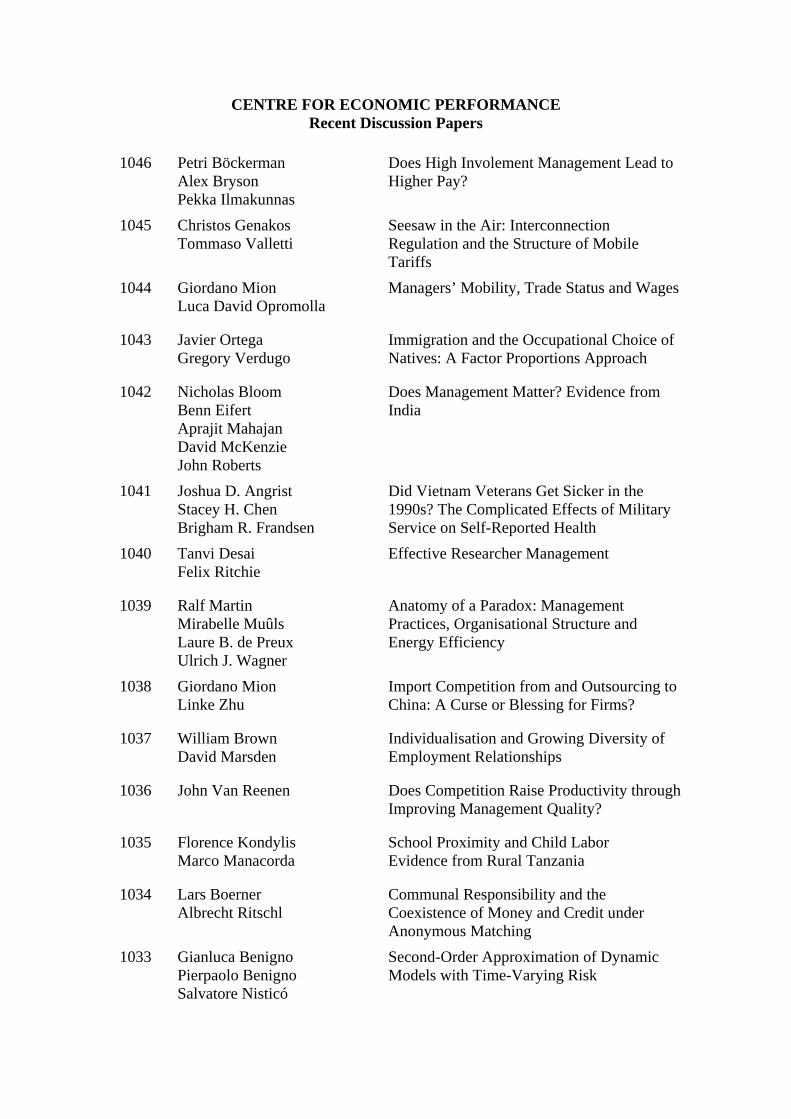
CENTRE FOR ECONOMIC PERFORMANCE Recent Discussion Papers

1046 Petri Böckerman Alex Bryson Pekka Ilmakunnas

Does High Involement Management Lead to Higher Pay?

1045 Christos Genakos Tommaso Valletti

Seesaw in the Air: Interconnection Regulation and the Structure of Mobile Tariffs

1044 Giordano Mion Luca David Opromolla

Managers’ Mobility, Trade Status and Wages

1043 Javier Ortega Gregory Verdugo

Immigration and the Occupational Choice of Natives: A Factor Proportions Approach

1042 Nicholas Bloom Benn Eifert Aprajit Mahajan David McKenzie John Roberts

Does Management Matter? Evidence from India

1041 Joshua D. Angrist Stacey H. Chen Brigham R. Frandsen

Did Vietnam Veterans Get Sicker in the 1990s? The Complicated Effects of Military Service on Self-Reported Health

1040 Tanvi Desai Felix Ritchie

Effective Researcher Management

1039 Ralf Martin Mirabelle Muûls Laure B. de Preux Ulrich J. Wagner

Anatomy of a Paradox: Management Practices, Organisational Structure and Energy Efficiency

1038 Giordano Mion Linke Zhu

Import Competition from and Outsourcing to China: A Curse or Blessing for Firms?

1037 William Brown David Marsden

Individualisation and Growing Diversity of Employment Relationships

1036 John Van Reenen Does Competition Raise Productivity through Improving Management Quality?

1035 Florence Kondylis Marco Manacorda

School Proximity and Child Labor Evidence from Rural Tanzania

1034 Lars Boerner Albrecht Ritschl

Communal Responsibility and the Coexistence of Money and Credit under Anonymous Matching

1033 Gianluca Benigno Pierpaolo Benigno Salvatore Nisticó

Second-Order Approximation of Dynamic Models with Time-Varying Risk

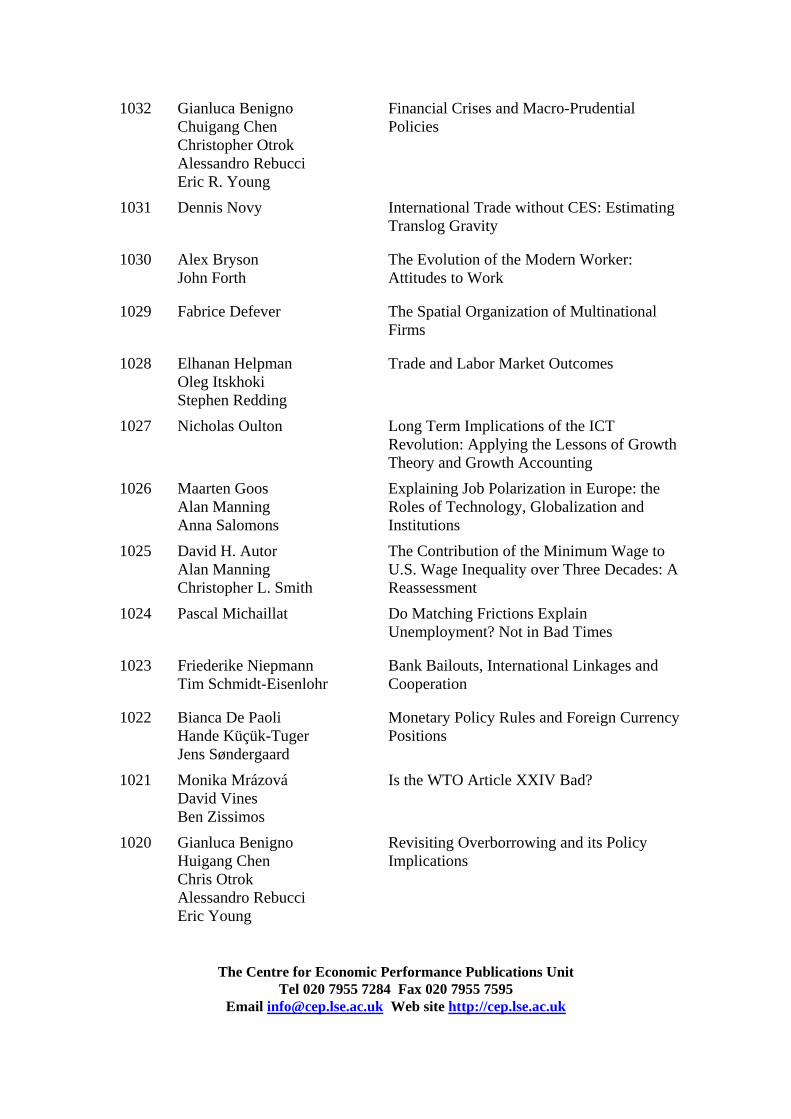
1032 Gianluca Benigno Chuigang Chen Christopher Otrok Alessandro Rebucci Eric R. Young

Financial Crises and Macro-Prudential Policies

1031 Dennis Novy International Trade without CES: Estimating Translog Gravity

1030 Alex Bryson John Forth

The Evolution of the Modern Worker: Attitudes to Work

1029 Fabrice Defever The Spatial Organization of Multinational Firms

1028 Elhanan Helpman Oleg Itskhoki Stephen Redding

Trade and Labor Market Outcomes

1027 Nicholas Oulton Long Term Implications of the ICT Revolution: Applying the Lessons of Growth Theory and Growth Accounting

1026 Maarten Goos Alan Manning Anna Salomons

Explaining Job Polarization in Europe: the Roles of Technology, Globalization and Institutions

1025 David H. Autor Alan Manning Christopher L. Smith

The Contribution of the Minimum Wage to U.S. Wage Inequality over Three Decades: A Reassessment

1024 Pascal Michaillat Do Matching Frictions Explain Unemployment? Not in Bad Times

1023 Friederike Niepmann Tim Schmidt-Eisenlohr

Bank Bailouts, International Linkages and Cooperation

1022 Bianca De Paoli Hande Küçük-Tuger Jens Søndergaard

Monetary Policy Rules and Foreign Currency Positions

1021 Monika Mrázová David Vines Ben Zissimos

Is the WTO Article XXIV Bad?

1020 Gianluca Benigno Huigang Chen Chris Otrok Alessandro Rebucci Eric Young

Revisiting Overborrowing and its Policy Implications

The Centre for Economic Performance Publications Unit Tel 020 7955 7284 Fax 020 7955 7595

Email info@cep.lse.ac.uk Web site http://cep.lse.ac.uk