Embed Size (px)
Citation preview
CEO Wage Dynamics:Estimates from a Learning Model
Lucian A. Taylor*
February 10, 2012
Abstract: The level of CEO pay responds asymmetrically to good and bad news about the
CEO’s ability. The average CEO captures approximately half of the surpluses from good
news, implying CEOs and shareholders have roughly equal bargaining power. In contrast,
the average CEO bears none of the negative surplus from bad news, implying CEOs have
downward rigid pay. These estimates are consistent with the optimal contracting benchmark
of Harris and Holmstrom (1982) and do not appear to be driven by weak governance. Risk-
averse CEOs accept significantly lower compensation in return for the insurance provided
by downward rigid pay.
JEL codes: D83, G34, M12, J31, J33, J41
Keywords: CEO, compensation, learning, dynamics, bargaining, SMM
Note: The Internet Appendix is at the end of this document but can eventually liveelsewhere.
* The Wharton School, University of Pennsylvania. Email: [email protected]. Iam grateful for comments from Chris Armstrong, Philip Bond, Alex Edmans, Carola Fryd-man (discussant), Itay Goldstein, Mariassunta Giannetti (discussant), Wayne Guay, AndreKurmann, Michael Lemmon, Evgeny Lyandres (discussant), Bang Nguyen, Kasper Nielsen,Gordon Phillips (discussant), Michael Roberts, Alexi Savov (discussant), Motohiro Yogo,and seminar participants at Carnegie Mellon University, Duke University, Laval University,University of Amsterdam, University of Pennsylvania, University of Utah, Yale University,the European Finance Association Meeting (2011), the FIRS Conference (2010), the Jack-son Hole Finance Conference (2011), the Olin Conference on Corporate Finance (2011), theRothschild Caesarea Center Conference (2010), the Society for Economic Dynamics Confer-ence (2010), and the Western Finance Association Meeting (2011). I am grateful for financialsupport from the Rodney L. White Center for Financial Research.
I. Introduction
There is considerable debate over the level of executive pay. One on side, Bebchuk and Fried
(2004) and others argue that weak governance allows executives to effectively set their own
pay while disregarding market forces and shareholder value. On the other side, Gabaix and
Landier (2008) and others argue that executive pay is determined in a competitive labor
market, so executives have limited influence on their own pay.
This paper uses CEO wage dynamics as a laboratory for exploring this debate. Specifi-
cally, I examine how learning about the CEO’s ability affects the level (i.e. expectation) of
the CEO’s pay. For example, a CEO’s perceived ability may increase after his firm delivers
high profits. This in turn increases the firm’s expected future profits, since high-ability CEOs
generate higher profits on average. The increase in expected profits is a positive surplus. How
the CEO and shareholders split this surplus depends on their relative bargaining positions,
which in turn depend on governance strength, contractual constraints, and outside options
in the labor market. For instance, the CEO may be able to capture the positive surplus by
bargaining for higher future compensation, as long as the CEO can make a credible threat to
leave the firm, the firm cannot make a credible threat to replace the CEO, and renegotiating
the CEO’s contract is not too costly. This paper’s goal is to measure the surpluses that
result from learning, and also to measure how the CEO and shareholders split them. The
estimates allow us to gauge CEOs’ influence over their own compensation.
Measuring the surpluses from learning presents a challenge, since we cannot directly ob-
serve perceived CEO ability, and since compensation and stock prices depend endogenously
on perceived ability. These challenges lend themselves to a structural estimation approach,
which infers unobservable quantities directly from endogenous patterns in the data. I es-
timate a model in which the CEO and shareholders gradually learn the CEO’s ability by
observing the firm’s profits and an additional, latent signal. Stock prices, return volatility,
and changes in the level of CEO pay respond endogenously to news about CEO ability.
1

I estimate the model’s five parameters using the simulated method of moments (SMM).
Separate parameters control how the CEO and shareholders split positive surpluses (from
good news) and negative surpluses (from bad news). Estimation uses data on excess stock
returns and total CEO compensation (including stock and option grants) for 4,545 Execu-
comp CEOs. I estimate the five parameters by matching 12 moments. The first 10 moments
measure how excess stock return volatility varies with CEO tenure, and the last two mea-
sure the sensitivity of changes in the level of CEO pay to positive and negative lagged excess
stock returns. The model fits these moments well, including the observed decline in return
volatility with CEO tenure, first documented by Clayton, Hartzell and Rosenberg (2005).
The paper’s main result is that the level of pay responds asymmetrically to good and
bad news about CEO ability: the average CEO bears none of the negative surplus resulting
from bad news about ability, whereas he or she captures roughly half of the surplus from
good news. One reason I find this result is that observed changes in the level of pay are
more sensitive to positive than negative lagged excess stock returns.
Since the level of CEO pay does not fall after bad news about ability, CEOs have down-
ward rigid pay.1 Shareholders, not the CEO, bear the negative surpluses from bad news
about the CEO’s ability. Downward rigid pay is consistent with the optimal contracting
benchmark of Harris and Holmstrom (1982). A long-term contract promising that the level
of pay will never drop is optimal in their model, because workers are risk-averse, whereas the
firm is risk neutral and hence can cheaply provide insurance against bad news. Downward
rigid pay therefore does not necessarily imply weak governance. Indeed, I find that pay is
downward rigid even in the subsample with high institutional ownership, a proxy for strong
governance. Pay is slightly more downward rigid, although not significantly so, when the
CEO has an explicit contract, also suggesting that the result is due to contracting rather
than governance. Downward rigid pay is pervasive across subsamples formed on firm size,
1This result is about the level of pay, which is the CEO’s expected compensation each year. A CEO’srealized pay can decrease over time due to the random incentive component of compensation.
2

industry, calendar year, and ten other characteristics. Downward rigid pay is also pervasive
in non-CEO occupations (e.g. Baker, Gibbs, and Holmstrom (1994), Dickens et al. (2007)).
According to Harris and Holmstrom (1982), CEOs accept lower average pay in return
for the insurance provided by downward rigidity, which saves the firm money. To quantify
these savings, I ask how much higher CEO pay would have to be to keep CEOs indifferent
between their actual, downward rigid compensation paths and counterfactual paths that are
not downward rigid. If CEOs’ relative risk aversion is 0.5 (4.0), first-year pay must increase
by a multiple of 1.3 (11.8), and the net present cost to the firm of five years of CEO pay
would increase by a multiple of 1.003 (8.1). If CEOs are sufficiently risk averse, the firm’s
savings from offering downward rigid pay are considerable.
Since CEOs capture roughly half of the positive surplus from good news, CEOs and
firms appear to have roughly equal bargaining power on average. In contrast, the models
of Jovanovic (1979), Harris and Holmstrom (1982), and Gibbons and Murphy (1992) all
predict that workers capture 100% of the surplus from good news, because they can always
threaten to take their ability to another firm at no cost. The estimates here suggest that
the average CEO’s actual outside employment options are not as strong as these models
assume. CEOs’ share of positive surpluses is significantly higher in the subsample with more
institutional ownership, implying that strong CEO bargaining power is not inconsistent
with strong governance. CEOs’ share of positive surpluses is also higher in subsamples
with insider CEOs and heterogeneous industries, potentially because their firms have fewer
potential replacement CEOs and hence less bargaining power. After controlling for multiple
characteristics, CEOs’ share of positive surpluses is positively related to the number of
similarly sized firms in the industry, a proxy for CEOs’ outside employment options.
Across industries, CEOs’ estimated share of positive surpluses ranges from 18% in Busi-
ness Equipment to 77% in Shops. CEOs capture just 19% of positive surpluses in the finance
industry, where the debate on executive pay has been especially contentious. This result im-
3

plies that financial firms’ shareholders, not their CEOs, are the main beneficiaries of good
news about their CEOs’ ability.
For robustness, I show that extended models with endogenous CEO firings, gradual vest-
ing of CEO pay, learning about firm quality, and persistent shocks to firm profitability pro-
duce slightly different parameter estimates. The average CEO’s estimated share of positive
surpluses ranges from 44 to 68%. Pay is downward rigid in all specifications. An important
caveat is that CEOs may be fired after enough bad news, so CEOs do bear personal costs
from bad news about their ability. While important and interesting in their own right, these
personal costs are unrelated to how CEOs and their current shareholders split the CEO’s
surplus, which is this paper’s focus.
My model is a simplified version of the learning models by Jovanovic (1979), Harris and
Holmstrom (1982), Murphy (1986), Gibbons and Murphy (1992), and Holmstrom (1999).2
This paper’s contribution is not to provide new predictions or further tests of existing pre-
dictions. Instead, the contribution is to quantify the surpluses from learning and measure
how they are shared, which sheds light on CEOs’ bargaining power. The paper therefore
complements existing empirical work that tests these models’ directional, reduced-form pre-
dictions but reveals less about underlying economic magnitudes.3 For example, Boschen and
Smith (1995) find a positive correlation between pay and lagged stock returns. Without a
structural model it is difficult to judge from their correlation whether CEOs capture 1%,
10%, or even 100% of positive surpluses. (I find they capture roughly 50%.) Whether CEOs
capture 1% or 100% has very different implications for CEOs’ bargaining power. Also, the
structural approach allows me to address an interesting counterfactual question: How much
more would firms have to pay CEOs if their pay were not downward rigid?
Like this paper, Gabaix and Landier (2008) and Tervio (2008) also measure how CEOs
2Milbourn (2003) also models CEO pay and learning about ability, but his goal is to explain cross-sectionalvariation in stock-based compensation.
3See Murphy (1986), Gibbons and Murphy (1992), Clayton, Hartzell, and Rosenberg (2005), Boschenand Smith (1995), and Cremers and Palia (2011).
4

and shareholders split the CEO’s surplus. Their evidence comes from the cross section,
whereas my evidence comes from the time series. Gabaix and Landier find that CEOs
capture only 2% of the value they create. Alder (2009) applies different functional forms
and finds a capture rate higher than Gabaix and Landier’s. Tervio (2008) finds that CEOs
capture roughly 20% of the value they add to their firms. Examining stock returns around
CEO deaths, Nguyen and Nielsen (2010) conclude that executives capture 80% of their
surplus. Whereas the previous papers measure CEOs’ total surplus, this paper measures
the surpluses created by news arriving each year, which allows me to distinguish between
positive and negative surpluses.
The paper makes one modest methodological contribution. Allowing parameter values
to vary with observable characteristics is rare in the structural corporate finance literature,
probably due to computational costs.4 Taylor (2010) and Nikolov and Whited (2009) cir-
cumvent the problem by estimating in subsamples, which makes it difficult to control for
several characteristics at once. I develop a method that solves this problem with minimal
computational costs. The method can apply to any project using GMM or SMM estimation.
The paper is structured as follows. Section 2 presents the learning model’s assumptions
and discusses identification. Section 3 describes the data and estimator. Section 4 presents
parameter estimates and results on model fit. Section 5 quantifies the value of downward
rigid pay. Section 6 describes how the parameters vary with firm, CEO, and industry char-
acteristics. Section 7 discusses robustness, and Section 8 concludes.
4Notable exceptions include Morellec, Nikolov, and Schuerhoff (2008), Korteweg and Polson (2009), Al-buquerque and Schroth (2010), and Dimopoulos and Sacchetto (2011). Hennessy and Whited (2005, 2007)use firm and year fixed effects to remove heterogeneity from the data before estimating.
5

II. The Dynamic Model of CEO Pay
The model features CEOs with different ability levels, meaning they can produce different
average firm-specific profitability. Neither CEOs nor shareholders can observe a CEO’s true
ability. Instead, they learn about ability over time by observing the firm’s realized profits
and a shared, additional signal. When a CEO’s perceived ability changes, so does his or her
perceived contribution to future firm profits. This change is a surplus, which the CEO and
shareholders split according to parameters θup and θdown.
Despite its simplicity, the model still allows me to empirically identify the magnitude of
surpluses from learning and how they are split. In Section 7 I extend the model to include
endogenous CEO firings, learning about firm quality, and persistent profitability shocks. I
show that these extended models produce similar estimates. I focus on the simpler model
here, because the intuition, solution, and estimation results are more transparent.
A. Assumptions
The model features firms i that live an infinite number of years t.
Assumption 1: The gross profitability (profits before CEO pay, divided by assets) of
firm i realized at the end of year t equals
Yit = ai + ηi + vt + εit. (1)
The unobservable ability of the CEO in firm i at time t is ηi, which is constant over the
CEO’s tenure. To be precise, ηi should have a CEO-specific subscript, since different CEOs
within the firm can have different abilities. Parameter ai, which will drop out of the analysis,
reflects the contribution of non-CEO factors in firm i. For now I assume ai is known and
constant. Shock vt has conditional mean zero; this shock is common to all firms in the
6

industry. Shock εit is an unobservable i.i.d. firm-specific shock distributed as N (0, σ2ε).
There are very many firms in the same industry as firm i, which implies that the industry
shock vt is observable even though ηi and εit are not.
Assumption 2: Investors use exogenous discount factor β to discount future dividends.
The firm immediately pays out any cash flows, including negative cash flows, as dividends.
This assumption allows me to solve for the firm’s market value. It improves tractability
by making the firm’s book assets constant over time.5
CEO j spends a total of Tj years in office. Tj is exogenous and known when the CEO
is hired.
Assumption 3: Agents have common, normally distributed prior beliefs about the
ability of a newly hired CEO in firm i: ηi ∼ N (m0i, σ20).
Different firms i may hire from different CEO talent pools, so the prior mean ability of
CEOs, m0i, is firm specific. The prior mean m0i will drop out of the analysis.
Assumption 4: Investors use Bayes’ Rule to update beliefs about CEO ability ηi af-
ter each year. They update their beliefs by observing the firm’s profitability Yit and an
additional, latent, orthogonal signal zit that is distributed as zit ∼ N (ηi, σ2z) .
The additional signal z represents information unrelated to current profitability, pos-
sibly from the CEO’s specific actions and choices, the performance of individual projects,
the CEO’s strategic plan, the firm’s growth prospects, discretionary earnings accruals, and
media coverage. I include this additional signal for two reasons. First, there is evidence
that investors use signals besides profitability when learning about CEO ability (Cornelli,
Kominek, Ljungqvist (2010)). Second, the additional signal helps the model fit certain fea-
tures of the data, as I explain later. The additional signal z is more precise when its volatility
5This assumption has little effect on the estimation results, since identification does not rely on changesin firm size, and since I use data on stock returns rather than earnings or cash flows.
7

σz is lower.
Assumption 5: Realized total compensation for the CEO in firm i and year t equals
wit = Et[wit] + bitrit. (2)
Realized pay is the sum of its level (Et[wit], known at the beginning of t) and a random
component that depends on the firm’s firm’s endogenous industry-adjusted stock return
(rit) and the CEO’s contemporaneous pay-performance sensitivity (bit).
The model makes predictions about changes in the level of CEO pay, and I use these
predictions to estimate the model. The contemporaneous pay-performance sensitivity bit
represents the incentive component of pay and depends on the CEO’s bonus and holdings
of stock and options. I treat this sensitivity bit as exogenous, for four reasons. First, I
do not need predictions about bit to estimate the model. Second, making bit endogenous
does not materially change the model’s predictions about the changes over time in expected
pay. Gibbons and Murphy (1992) make bit endogenous by incorporating moral hazard, effort
choice, and optimal contracts into a model of learning about an executive’s ability. They
show that the optimal contract sets the contemporaneous pay-performance sensitivity so
that the CEO exerts optimal effort. The contract sets expected pay so that the CEO agrees
to stay in the firm rather than leave to some outside option. More importantly, they show
that making bit endogenous does not significantly change the model’s predictions about the
change over time in a CEO’s expected pay. Third, modeling bit in a reduced-form manner
allows it to depend flexibly on firm and CEO characteristics. Of course, making bit exogenous
significantly simplifies the model solution and estimation.
8

Assumption 6: The change in the level of pay is
∆Et [wit] ≡ Et [wit]− Et−1 [wit−1] (3)
= θtBi (Et [ηi]− Et−1 [ηi]) (4)
θt = θup if Et [ηi] ≥ Et−1 [ηi] (beliefs increase) (5)
θt = θdown if Et [ηi] < Et−1 [ηi] (beliefs decrease). (6)
By equation (1), the CEO’s expected contribution to firm profits (in dollars) in year
t is BiEt [ηi], where Bi is the firm’s assets. The change in this expected contribution is
Bi(Et[ηi] − Et−1[ηi]). This quantity is the surplus created by news in year t − 1 about the
CEO’s ability. Assumption 6 therefore states that the CEO captures a fraction θt of the
change in his expected contribution to firm profits. When beliefs increase (decrease), the
CEO captures a fraction θup (θdown) of this surplus. The parameters θup and θdown measure
the CEO’s bargaining power over changes in the level of pay. This assumption follows the
literature’s practice of assuming that a surplus is split according to a constant, exogenous
parameter (e.g. Morellec, Nikolov, and Schurhoff (2010)).
Assumption 6 nests the reduced-form predictions from several existing theories with
stronger micro foundations, which I summarize below. Adding these theories’ micro foun-
dations would constrain θup and θdown but not otherwise change Assumption 6. Estimating
θup and θdown allows me to compare the data to these theories’ predictions.
The theories below illustrate that there are several economic factors that affect how CEOs
and shareholders split surpluses. This paper’s main goal is not to measure the relative impor-
tance of these and other factors, but to measure their total effect on CEO bargaining power.
However, Section 6 takes initial steps toward comparing the various factors by measuring
how my estimates vary cross-sectionally.
A special case of the model is when the CEO’s expected pay exactly equals the CEO’s
9

expected contribution to firm profits (BiEt[ηi]) every year. This special case matches the
predictions from the equilibrium learning models of Jovanovic (1979), Gibbons and Murphy
(1992), and Holmstrom (1999). I summarize the assumptions of Gibbons and Murphy (1992)
to provide micro foundations for this special case. They assume that every period there
are multiple identical firms competing for the CEO. The firms offer the CEO single-period
contracts, and the CEO chooses his or her preferred contract. The CEO’s outside option
is to work at one of these firms, and the firm’s outside option is to hire a new CEO whose
ability is a random draw from the talent pool. The equilibrium level of pay therefore equals
the CEO’s perceived contribution to the firm every year. As a result, the CEO captures
θup = θdown = 100% of the surplus from learning. Later, I show that the data are not
consistent with this benchmark.
As discussed earlier, Harris and Holmstrom (1982) provide a second micro foundation
with optimal contracts. Their model predicts that the CEO’s expected pay never drops
(θdown = 0), but the CEO has strong enough outside options to capture 100% of positive
surpluses (θup = 1). I show that the data are closer to this benchmark.
Other models omit learning but focus on labor market frictions that affect bargaining
power. If the CEO’s human capital is specific to the firm, then the CEO possibly cannot make
a strong threat to leave firm, hence the CEO captures less of a positive surplus (Murphy and
Zabojnik, 2007). If the CEO’s outside option is to work in a smaller firm, as in the matching
models of Gabaix and Landier (2008) and Tervio (2008), then the CEO’s outside option and
bargaining power are weaker. If the CEO would lose unvested shares and options by leaving
the firm, the CEO’s bargaining position is weaker.
B. Model Solution and Identification
Next, I summarize the model’s predictions and provide intuition for how the estimation
procedure identifies parameter values from the data. Closed-form solutions and proofs are
10

in the Internet Appendix.6
The first predictions are about the volatility of excess stock returns. The model predicts
that return volatility decreases with CEO tenure. The reason is that uncertainty about CEO
ability contributes to uncertainty about dividends, and this uncertainty gradually decays to
zero as investors learn. Return volatility eventually reaches a level that depends only on
σϵ, the volatility of shocks to profitability. Data on return volatility for long-tenured CEO
therefore identify parameter σϵ.
Parameter σz, the additional signal’s noise, is mainly identified off how quickly return
volatility drops with CEO tenure. Return volatility drops faster when σz is lower, meaning
the additional signal zit is more precise. The reason is that a more precise signal allows
agents to learn the CEO’s ability more quickly. A more precise signal also increases return
volatility in the CEO’s first year, because beliefs about the CEO and hence stock prices
move more during that year.
The amount by which stock return volatility drops is (i) increasing in the amount of prior
uncertainty about CEO ability (σ0), but (ii) decreasing in CEOs’ share of the surplus (θup
and θdown). The intuition for (i) is that if uncertainty about the CEO has farther to drop,
so does return volatility. Return volatility does not drop at all if there is no uncertainty
about the CEO (σ0 = 0). The intuition for (ii) is that there is more uncertainty about
dividends if CEOs capture a smaller share (and hence shareholders capture a larger share)
of the surpluses from news about ability.
The next predictions are about the relation between CEO pay and stock returns. The
model predicts a positive relation between changes in expected pay and the firm’s lagged
excess stock return, consistent with the empirical evidence of Boschen and Smith (1995).
To see why, suppose the firm experiences higher than expected profits in year t − 1. This
has two effects: a positive excess stock return in year t − 1, and an increase in the CEO’s
6The Internet Appendix is currently attached to this document. Eventually it can live on the Internetsomewhere.
11

perceived ability, which in turn makes expected CEO pay higher in year t than t− 1.
The sensitivity of expected pay to lagged returns depends on θup when surpluses are posi-
tive and on θdown when surpluses are negative. Positive surpluses typically (but not always7)
coincide with positive excess stock returns. As a result, the sensitivity of changes in expected
CEO pay to positive lagged excess returns is most informative about θup. Conversely, the
sensitivity of pay to negative returns is most informative about θdown. The sensitivities of
CEO pay to positive and negative lagged returns will help to disentangle θup and θdown in
the estimation procedure.
The predicted sensitivity of pay to lagged returns increases in both prior uncertainty (σ0)
and the CEO’s share of the surplus (θt). When there is more prior uncertainty, beliefs move
more in response to any given signal. The surpluses are therefore larger in magnitude, so
the changes in CEO pay are also larger. Expected CEO pay moves more with lagged stock
returns when θt is higher, because the CEO captures a larger fraction of the surpluses.
INSERT FIGURE 1 HERE
Figure 1 illustrates how the predictions above allow us to separately identify prior uncer-
tainty (σ0) and the CEO’s share of the surplus (θt) from the data. The key is that these two
parameters have different predicted effects on (a) the drop in return volatility and (b) the
sensitivity of pay to lagged returns. To simplify the explanation, suppose θup = θdown = θ.
The solid line shows the infinitely many combinations of σ0 and θ that allow the model to
match a given, observed drop in return volatility. The line slopes up, because the predicted
drop in return volatility is increasing in σ0 but decreasing in θ, as explained above. The
dashed line shows the infinitely many combinations of σ0 and θ that allow the model to fit a
given, observed sensitivity of CEO pay to lagged returns. The line slopes down, because the
predicted sensitivity is increasing in both σ0 and θ (also above). The lines’ opposite slopes
make them cross at a unique point {σ0, θ}. The estimation procedure will find this unique
7If the additional signal zit is high enough, the CEO’s perceived ability and pay level can increase evenif the profitability shock and excess return are zero or negative.
12

point that lets the model simultaneously match both moments.
III. Estimation
A. Data
Data come from Execucomp; CRSP; Compustat; Kenneth French’s website; Thomson Fi-
nancial; Risk Metrics; Gillan, Hartzell, and Parrino (2009); Peters and Wagner (2009); and
Jenter and Kanaan (2011).8 The sample includes CEOs in the Execucomp database from
1992 to 2007. Execucomp includes S&P 1500 firms, firms removed from the S&P 1500 that
are still trading, and some client requests. The Internet Appendix provides details on how I
construct the sample.
Excess return rit is the firm’s annual stock return minus the equal-weighted Fama French
49 industry return. I account for firms’ fiscal calendars when computing fiscal year returns.
The measure of CEO pay is Execucomp’s TDC1, which includes each year’s salary, bonus,
total value of restricted stock granted, total value of stock options granted (using Black-
Scholes), long-term incentive payouts, “other annual,” and “all other total.” A plausible
interpretation of the model is that the firm and CEO renegotiate the labor contract at the
beginning of each year. The contract sets expected pay in the coming year to the level that
induces the CEO to remain at the firm and work throughout year t. The benefit of using
TDC1 is that it excludes stock and options that were granted and vested in past years, which
are sunk and therefore should not affect the CEO’s decision to stay in the firm in the current
year. For robustness, in Section 7 I use an alternate measure that includes stock and options
in the year they vest. Estimation uses data on the change in realized CEO pay, divided by
lagged market cap. I winsorize this variable at the 1st and 99th percentiles.
8I thank these authors for generously sharing their data.
13

I measure the annual variance of excess stock returns by taking the variance of weekly
industry-adjusted stock returns during each firm’s fiscal year, then multiplying by 52 to
annualize. I winsorize this variable at the 1st and 99th percentiles.
Another estimation input is Tj, the total years CEO j spends in office. If Tj is known
(i.e. CEO’s last year in office is in Execucomp) then I use the actual value. If Tj is not
known (i.e. CEO’s last year is not in Execucomp), then I forecast it using the CEO’s age
and tenure from his last observation in the database; details are in the Internet Appendix.
INSERT TABLE 1 HERE
Summary statistics are in Table 1 . The database contains 20,700 firm/year observations
and 4,545 CEOs. Mean realized pay is $4.13 million, with a standard deviation of $5.60
million. A CEO’s realized pay fluctuates considerably over time: the change in realized pay,
as a fraction of lagged market cap, has a standard deviation of 0.40%. The median firm/year
observation is for a CEO in his 6th year in office. The median firm has $1.27 billion in assets
and a market capitalization of $1.16 billion. Section 6 discusses the remaining variables in
Table 1.
B. Estimator
I estimate the five model parameters in Θ =
[σ2ε σ2
z σ20 θup θdown
]using SMM.9 The
estimator is
Θ ≡ argminΘ
(M− m (Θ)
)′W(M− m (Θ)
). (7)
M is a vector of moments estimated from the actual data, and m (Θ) is the corresponding
vector of model-implied moments. The hat on m indicates that some model-implied moments
are estimated by simulation. For these simulations, I use parameter values Θ to simulate
a sample many times larger than the empirical sample, then I compute the moment from
9See, for instance, Strebulaev and Whited (2012).
14

simulated data in the same way I compute the empirical moment. I set W equal to the
efficient weighting matrix, which is the inverse of the estimated covariance of moments M.
I estimate the five parameters in Θ using 12 moments in vectors M and m. The first
moment is the average variance of excess returns for CEOs in their first year in office.
Moments 2–10 measure how return volatility varies with CEO tenure. Specifically, using
firm/year data I regress the variance of excess stock returns on nine dummy variables for
CEO tenure equal to 2, ..., 9, and 10+ years; the log of the firm’s lag assets; the log of firm
age; and industry × year fixed effects.10 The slopes on the nine CEO tenure dummies make
up moments 2–10.
The 11th and 12th moments are the slopes M (11) and M (12) from a regression of scaled
changes in expected pay on positive and negative lagged excess returns as well as an indicator
for the lagged return’s sign:
∆Et [wit]
Mit−1
= a0 + a11 (rit−1 > 0) +M (11)r(+)it−1 +M (12)r
(−)it−1 + eit, (8)
where r(+)it−1 = rit−1 if rit−1 ≥ 0 and equals zero otherwise; vice-versa for r
(−)it . Estimating (8) is
straightforward using simulated excess returns and changes in expected pay. To estimate (8)
using actual data on realized pay, first I parameterize the contemporaneous pay-performance
sensitivity bit from Assumption 5 as
bit = Mitb(+) if rit ≥ 0 (9)
= Mitb(−) if rit < 0, (10)
where b(+) and b(−) are nuisance parameters to be estimated. This parametrization takes into
account that dollar changes in CEO pay are larger in larger firms, and that firms may set
10I include the control variables and fixed effects so that the slopes on the CEO tenure dummies do notsimply capture correlated changes in firm size, firm age, or unobserved heterogeneity across industry/years.Hennessy and Whited (2005, 2007) also used fixed effects to remove heterogeneity from the data beforeestimating.
15

different sensitivities to positive and negative contemporaneous returns. I substitute these
equations into (8) to derive a regression model for changes in realized pay:11
∆wit
Mit−1
= a0 + a11 (rit−1 > 0) + λ11r(+)it−1 + λ12r
(−)it−1 (11)
+b(+)
[Mit
Mit−1
r(+)it
]+ b(−)
[Mit
Mit−1
r(−)it
]+ eit
λ11 = M (11) − b(+) (12)
λ12 = M (12) − b(−). (13)
I estimate this regression by OLS and then estimate the last two moments as
M11 = λ11 + b(+) (14)
M12 = λ12 + b(−). (15)
This procedure accounts for the estimation error in nuisance parameters b(+) and b(−) when
measuring the error in moments M (11) and M (12).
IV. Estimation Results
I begin by describing how the model fits the data. I then present the main parameter
estimates, which characterize the average firm and CEO. In section 6 I describe how the
parameter estimates vary across firms and CEOs.
11Assumption 5 implies Et [wit] = wit − bitrit, so equation (8) implies
wit − bitrit − (wit−1 − bit−1rit−1)
Mit−1= a0 + a11 (rt−1 > 0) +
M (11)r(+)it−1 +M (12)r
(−)it−1 + eit.
Rearranging terms and substituting equation (9) yields equation (11).
16

A. Model Fit
Panel A of Table 2 contains actual and simulated values of the 12 moments used in the
SMM estimation along with t-statistics testing their difference. The model closely matches
the level of return volatility in CEOs’ first year in office and also the tenure fixed effects in
return volatility. Figure 2 plots these fixed effects to make interpretation easier. In both the
actual data (dashed line) and simulated data (solid line), return volatility drops rapidly in
CEOs’ first three years in office, indicating that agents learn the CEO’s ability quite fast.
The model fits the timing and magnitude of these changes remarkably well.
INSERT TABLE 2 HERE
INSERT FIGURE 2 HERE
Return volatility decreases with tenure in the model due to learning. Outside the model,
an alternate explanation for this decrease is that earnings volatility declines with tenure. In
the Internet Appendix I show there is no significant relation between CEO tenure and the
volatility of firm profitability. Also, I show that the decline in return volatility is robust to
controlling for the magnitude of the shock to profitability in the same firm and year.
The last two moments in Table 2 measure the sensitivity of changes in the pay level to
both positive and negative lagged excess returns. Both sensitivities are significantly positive,
and the model fits both almost exactly. The sensitivity to positive returns is more than 3
times larger than the sensitivity to negative returns. The result is not due to the convexity
of stock option payoffs, because the measure of CEO pay values options at their grant date,
not their payout or vesting dates.
Table 2 also presents the J-test of the model’s overidentifying restrictions. We cannot
reject the hypothesis that the model matches all 12 empirical moments (p=0.965). While
this result is good news for the model, we know that with enough additional data we will
surely reject any model, including this one.
17

Panel B of Table 2 illustrates this point by showing some features of the data that the
model fits less well. Specifically, I measure the inflation-adjusted change in a CEO’s realized
pay12 from year 1 to year 5 in office, scaled by the firm’s assets at the beginning of the
1st year. In both actual and simulated data, the median CEO’s pay level increases with
tenure, consistent with the empirical findings of Murphy (1986) and Cremers and Palia
(2011). Pay ratchets up over time in the model because, as explained below, CEOs avoid
negative surpluses but capture a large portion of positive surpluses. Pay increases even for
the simulated 25th percentile CEO, who receives mostly bad news about ability. This last
prediction is at odds with the data: the actual 25th percentile CEO sees pay decrease, albeit
by only 0.019% of firm assets. Also, the model generates larger changes in pay than we see in
the data: pay for the 75th percentile CEO increases by 1.65% of firm assets in the model but
only by 0.10% in the actual data. One potential explanation, which additional regressions
reject, is that the changes in expected pay correlated with lagged returns are transitory, not
permanent as the model assumes.13 Extending the model to accommodate these additional
features of the data is an interesting avenue for future work.
B. Main Parameter Estimates
Table 3 presents the main parameter estimates along with results from robustness specifica-
tions discussed in Section 7. The estimated standard deviation of profitability shocks (σε)
is 36% per year. The model needs this high value to match the high level of stock return
volatility. DeAngelo, DeAngelo, and Whited (2010) directly estimate the annual volatility
of innovations to profitability, and they find a much lower value, 7% per year. This paper’s
high estimate of σε reflects the well known excess volatility puzzle (Shiller, 1981): it is dif-
ficult to reconcile the high level of return volatility with the relatively low level of earnings
12Following equation (2), realized pay equals expected pay plus the pay-performance sensitivity bit (esti-mated in regression (11)) times the contemporaneous excess return.
13Specifically, I include rit−2 in regression (11) and find that its slope is indistinguishable from zero. Ifthe shocks were transitory then we should find a negative slope.
18

volatility. In Section 7 I show that we can interpret σε as the volatility of shocks to current
plus discounted future profitability, in which case an estimate of 36% makes more sense.
INSERT TABLE 3 HERE
The high estimate of σϵ implies that profitability is a very noisy signal of CEO ability.
The additional signal z is much less noisy, with an estimated volatility of 3.3% per year.
The precise z signal allows agents to learn quickly, which allows the model to fit the sharp
drop in return volatility during CEOs’ first three years in office. Consistent with these
results, Cornelli, Kominek, and Ljungqvist (2010) show that boards rely on soft information
in addition to firm performance when learning a CEO’s ability. Taylor (2010) finds that a
precise additional signal of CEO ability is needed to rationalize data on firm profitability
and CEO firings.
The estimated standard deviation of prior beliefs about CEO ability (σ0) is 4.1%. Using
this estimate, the difference in average profitability between CEOs at the 5th and 95th
ability percentiles is 2 × 1.65 × σ0 = 13.6% of assets per year, which is quite large. For
comparison, using a different data set and identification strategy, Taylor (2010) estimates a
2.4% standard deviation in prior beliefs about shareholders’ share of the surplus from CEO
ability. Not surprisingly, the prior uncertainty about the total surplus, which I measure in
this paper, is higher. Bertrand and Schoar (2003) estimate manager-specific fixed effects in
annual profitability. They find a 7% standard deviation in fixed effects across managers,
implying even greater dispersion in ability than reported here.
CEOs’ estimated share of a negative surplus (θdown) is -5.1%, indicating the level of pay
actually increases slightly following bad news. However, the estimate is not statistically
different from zero, so I cannot reject the hypothesis that CEO pay is perfectly downward
rigid. This result implies that shareholders, not the CEO, bear the entire negative surplus
resulting from bad news about a CEO’s ability. Since a negative value of θdown is somewhat
implausible ex ante, I re-estimate the model with the constraint θdown ≥ 0 (Table 3, “Con-
19

strained θ”). This constraint has little effect on the other parameter estimates or model fit.
I impose this constraint throughout the rest of the paper.
CEOs’ estimated share of a positive surplus (θup) is 48.9%. In other words, the level of
CEO pay changes 0.489 for one with increases in the CEO’s perceived contribution to firm
profits. CEOs and shareholders almost equally share the benefits from an improvement in
the CEO’s perceived ability.
In sum, I find that CEO pay responds asymmetrically to good and bad news. I can reject
the hypothesis that θup = θdown with a t-statistic of 3.9. The main reason I find θup > θdown
is that changes in CEO pay are more sensitive to positive lagged returns than to negative
lagged returns, as shown in Table 2.
V. How Valuable Is Downward Rigid Pay?
Downward rigid pay insures CEOs against bad news about their ability. According to
Harris and Holmstrom (1982), CEOs are willing to pay for this insurance by accepting lower
average compensation, which adds value to the firm. In this section I quantify the value of
this insurance to the CEO and firm by comparing the estimated model to a counterfactual
model without downward rigid wages.
I start by simulating compensation paths for the median sample firm using Table 3’s
parameter estimates. The main model only makes predictions about changes in pay. To
obtain predictions about the level of pay, I set CEOs’ average first-year pay to $2.84M, the
sample median in 2011 dollars. Panel A of Table 4 shows that simulated pay rarely decreases.
The simulated net present cost to the firm of five years of CEO pay is $55.3M.
INSERT TABLE 4 NEAR HERE
To gauge how CEO pay would change if it were not downward rigid, I compare the
20

compensation paths above to paths simulated from a counterfactual model that is identical
to the main model but assumes θdown = θup = 0.489. I solve for the level of first-year pay
that makes the CEO’s expected utility the same as in the base-case simulations above. In
other words, I ask how the starting level of pay must change to make the CEO indifferent
between having and not having downward rigid pay. I assume the CEO has constant relative
risk aversion preferences over realized pay in years one to five. I repeat the exercise using
risk aversion coefficients between 0.5 to 4.14
Simulated counterfactual results are in Panel B. Pay now decreases as often as it increases,
which by itself makes average future pay lower than in the base-case model. First-year pay
must increase to compensate the CEO for the lower average future pay. The larger spread
between the 25th and 75th percentile CEOs indicates that pay has also become riskier,
so first-year pay must increase even more to compensate CEOs for this added risk. With
relative risk aversion set to 0.5, first-year pay increases from $2.84M to $13.1M, and the net
present cost of pay to the firm increases from $55.3M to $62.6M (a factor of 1.13). When
relative risk aversion increases from 0.5 to 4, the CEO requires more compensation for his
riskier pay, so first-year pay increases from $13.1M to $113.8M, and the net present cost to
the firm increases from $62.6M to $419.0M, 7.6 times higher than with downward rigid pay.
These costs of removing downward rigid pay are not trivial compared to the median sample
firm’s assets, $1.6 billion in 2011 dollars.
A potential concern is that pay is more volatile in the model than in the actual data
(recall Table 2), so the results above likely overestimate the value of downward rigid pay. To
address this concern, I repeat the exercise by bootstrapping actual data instead of simulating.
Specifically, I compare compensation paths sampled from their actual distribution (which
features downward rigid pay) and a counterfactual distribution constructed so that pay
decreases exactly as often as it increases. The counterfactual distribution includes all actual
14CRRA preferences cannot accommodate negative wages, which the model sometimes produces. I boundpay from below at $100K per year.
21

pay paths where 5th year pay exceeds 1st year pay, and also the mirror image of those same
paths.15 As before, I ask how much first-year pay must increase to make the CEO indifferent
between the actual and counterfactual compensations paths, the latter being both riskier
and lower, all else equal.
Panel C describes the empirically sampled paths. As expected, pay increases more often
than it decreases. The net present cost of 5 years of pay is $15.46M. Panel D describes the
counterfactual paths. With a risk aversion coefficient of 0.5, first-year pay must increase
from $2.84M to just $3.58M, and the net present cost of pay increases by just a multiple of
1.003. However, when the risk aversion coefficient increases to 4, first-year pay must increase
to $33.6M and the net present cost increases by $109M (a multiple of 8.1).
To summarize, the costs of eliminating downward rigid pay are not small if CEOs are
sufficiently risk averse. This exercise may push the model beyond its limitations. Holding
other parameters constant while varying θdown is especially aggressive. For instance, elimi-
nating downward rigid pay would likely change the risk aversion and prior uncertainty (σ0)
of those who choose to become CEOs, which in turn could affect firm value. This exercise
takes a first step toward valuing the insurance provided by CEOs’ downward rigid wages.
Hopefully future research will provide more refined estimates.
VI. CEO Wage Dynamics and the Cross Section
The results so far quantify the surpluses from learning and how they are shared for the
average CEO and firm. Now I begin exploring why surpluses are shared the way they are,
and why the surpluses have their observed magnitude. I do so by measuring how parameters
estimates vary in the cross section with proxies for governance strength, CEOs’ outside
15The mirror image paths start from the same first-year pay, but the subsequent changes in pay have theopposite sign as the actual data. As a result, 5th year pay is less than 1st year pay in the mirror imagepaths. As before, I bound pay from below by $100K, and I normalize all paths’ first-year pay to the samplemedian, $2.84M.
22

options, contractual constraints, and prior uncertainty. An important caveat is that all the
proxies are endogenous and I lack instruments, so the correlations below do not have a causal
interpretation.
I use five proxies for CEOs’ outside employment opportunities: the number of years the
CEO spends in the firm before becoming CEO (“insider” status, a proxy for firm-specific hu-
man capital), the fraction of industry CEOs promoted from within the firm, the homogeneity
of firms in the industry,16 the number of similarly sized firms in the same industry, and the
number of outside directorships the CEO holds. I also include two contracting variables that
may affect bargaining outcomes: the amount of unvested shares and options the CEO holds,
and an indicator for whether the CEO has an explicit employment agreement.17 The proxies
for prior uncertainty are the CEO’s age and insider status. I also include as control variables
the log of the firm’s lagged assets, the fraction of shares held by institutional investors (a
proxy for governance strength), and the log of the firm’s age. Detailed definitions of these
variables are in the Appendix, and summary statistics are in Table 1.
Next I describe the method for measuring how the model’s five parameters vary with
the characteristics above. The main idea is that the structural parameters vary with a
characteristic like firm size (for instance) only if the 12 moments M used in SMM estimation
vary with firm size. I use the following formula to measure the change in parameter estimates
Θ associated with a small change in characteristic Zj (e.g., firm size), holding constant other
characteristics Z∼j:
∂Θ
∂Zj
=∂Θ
∂M
∂M
∂Zj
. (16)
The right-hand side equals the parameter estimates’ sensitivity to moments’ values (com-
puted by perturbing each moment and re-estimating), times the moments’ sensitivity to
16This variable, which is from Parrino (1997) and Gillan, Hartzell, and Parrino (2009), equals the medianacross Execucomp firms in the same industry of the R2 from time-series regressions of monthly stock returnson equal-weighted industry portfolio returns.
17Data on employment agreements are from Gillan, Hartzell, and Parrino (2009). CEOs have an explicitemployment agreement in 42% of firm/year observations.
23

characteristics (computed in OLS regressions). The Appendix provides implementation de-
tails. Estimated sensitivities ∂Θ/∂Zj are in Table 5. I supplement these results by estimating
the model in subsamples formed on ten characteristics (Table 6).18 The benefit of the sub-
sample approach is that it measures the effect of large changes in characteristics, whereas
the approach in equation (16) only measures the effect of small, local changes. The benefit
of equation (16) is that, like a multiple regression, it controls for multiple characteristics at
once, whereas the subsample approach does not.
INSERT TABLE 5 NEAR HERE
INSERT TABLE 6 NEAR HERE
CEOs’ share of the surplus from good news (θup) is significantly higher in the subsamples
with insider CEOs, lower industry homogeneity, fewer directorships, smaller firms, higher
institutional ownership, and older firms. One interpretation is that insider CEOs in het-
erogeneous industries have more bargaining power, since their firms have fewer potential
replacement CEOs with similar expertise. Weak governance does not appear responsible for
CEOs capturing positive surpluses, since θup is actually higher when there is more institu-
tional ownership. After controlling for multiple characteristics in Table 5, the subsample
differences lose significance. Instead, we see CEOs capturing more of the positive surplus
in industries with more insider CEOs, possibly because their firms have fewer replacement
CEOs. There is also a positive relation between θup and the number of similarly sized firms
within the same industry, consistent with CEOs having a stronger bargaining position when
there are more firms where they could potentially work.
Parameter θdown is either constrained at zero or indistinguishable from zero in all 20
subsamples, indicating that downward rigid pay is pervasive. Weak governance does not
18The model is not well identified in subsamples based on whether the CEO has an explicit contract,because in both subsamples return volatility does not decline with tenure. This is a small-sample problem,as data on CEO contracts are missing in roughly 80% of the sample. I impose the estimation constraintσz ≥ 0.01, which binds in six of 20 subsamples in which the decline in return volatility occurs over just oneyear. Without this constraint the model is poorly identified in these six subsamples.
24

appear responsible for downward rigid pay, which is even more pronounced (although not
significantly so) when there is more institutional ownership (Table 5). Table 5 shows that
pay is also more downward rigid (although not significantly so) when the CEO has an explicit
contract, which is consistent with downward rigidity being a feature of optimal contracts, as
Harris and Holmstrom (1982) predict.
Prior uncertainty about ability (σ0) is significantly higher, and hence the surpluses from
learning are larger in magnitude, in the subsamples with outsider CEOs, more directorships,
smaller firms, and younger firms. After controlling for multiple characteristics in Table
5, only firm size remains significant, potentially because CEO ability matters more (as a
fraction of assets) in smaller firms, where the CEO necessarily delegates less. We also see a
negative relation between uncertainty and the fraction of industry CEOs who are insiders,
consistent with insiders being more of a “known quantity.” Uncertainty is not significantly
related to the CEO’s age, possibly because ability is match specific.
I also estimate the model in the sample’s largest four industries and in calendar year
subsamples (Table 7). Pay is downward rigid in all subsamples. CEOs’ share of positive
surpluses ranges from 18% in Business Equipment to 77% in Shops. CEOs capture just 19%
of positive surpluses in financial firms. CEOs’ share of positive surpluses has dropped from
57% in 1992–1997 to 34% in 1998–2007, but the change is not statistically significant. Prior
uncertainty (σ0) has increased significantly over time, indicating the surpluses from learning
have grown in magnitude.
The model fits the data well in all subsamples. The J-test cannot reject the model at
the 10% level in any of the 26 subsamples.
To summarize, weak governance, as in Bertrand and Mullainathan (2001), does not seem
to be driving the asymmetric response of pay to good and bad news. Downward rigid pay is
pervasive. Some proxies for bargaining power are intuitively correlated with θup, but other
proxies have either a counterintuitive or insignificant correlation. One possible explanation
25
is that the proxies are noisy. Another is that several of these variables proxy not just for
CEOs’ bargaining power but also for firms’ bargaining power, and these two effects offset
each other.19 Results are quite different depending on whether I estimate in subsamples or
control for multiple characteristics.
VII. Robustness
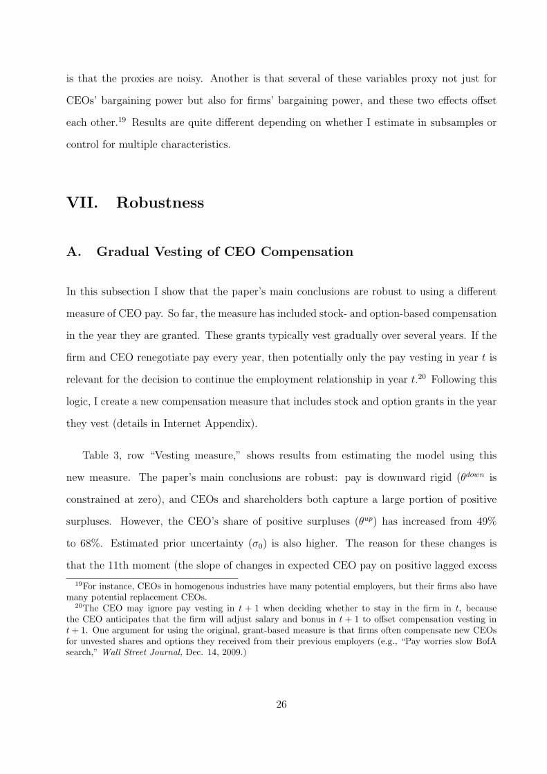
A. Gradual Vesting of CEO Compensation
In this subsection I show that the paper’s main conclusions are robust to using a different
measure of CEO pay. So far, the measure has included stock- and option-based compensation
in the year they are granted. These grants typically vest gradually over several years. If the
firm and CEO renegotiate pay every year, then potentially only the pay vesting in year t is
relevant for the decision to continue the employment relationship in year t.20 Following this
logic, I create a new compensation measure that includes stock and option grants in the year
they vest (details in Internet Appendix).
Table 3, row “Vesting measure,” shows results from estimating the model using this
new measure. The paper’s main conclusions are robust: pay is downward rigid (θdown is
constrained at zero), and CEOs and shareholders both capture a large portion of positive
surpluses. However, the CEO’s share of positive surpluses (θup) has increased from 49%
to 68%. Estimated prior uncertainty (σ0) is also higher. The reason for these changes is
that the 11th moment (the slope of changes in expected CEO pay on positive lagged excess
19For instance, CEOs in homogenous industries have many potential employers, but their firms also havemany potential replacement CEOs.
20The CEO may ignore pay vesting in t + 1 when deciding whether to stay in the firm in t, becausethe CEO anticipates that the firm will adjust salary and bonus in t + 1 to offset compensation vesting int+ 1. One argument for using the original, grant-based measure is that firms often compensate new CEOsfor unvested shares and options they received from their previous employers (e.g., “Pay worries slow BofAsearch,” Wall Street Journal, Dec. 14, 2009.)
26

returns) has increased from 0.0023 to 0.0053.21 To fit this higher sensitivity while fitting the
unchanged return volatility pattern, the model needs both larger surpluses (higher σ0) and
a larger share going to the CEO (higher θup).
B. Endogenous CEO Dismissals
The main model assumes CEOs are not fired after bad performance. There is considerable
evidence to the contrary, extending from Coughlan and Schmidt (1985) through Jenter and
Lewellen (2011). CEOs bear large, personal costs when they are fired: Fee and Hadlock
(2004) find that dismissed CEOs who go on to run another firm end up at firms that are
much smaller, which brings large decreases in compensation. While interesting and impor-
tant for CEO incentives, these personal costs are unrelated to how CEOs and their current
shareholders split the CEO’s surplus, which is this paper’s focus. Firing the CEO after bad
performance does not create a negative surplus, according to this paper’s definition. As soon
as the CEO and firm separate, the surplus the CEO brought to that firm ceases to exist, so
we can no longer measure how it is shared.
Ignoring dismissals may nevertheless introduce estimation bias. I address this concern
by estimating an extended model with endogenous firings. I follow the method of Taylor
(2010), adding the following assumptions to the main model. The board of directors decides
at the end of each year whether to fire or keep its CEO. An alternate interpretation is that
shareholders decide each year whether the company should be acquired, in which event the
CEO is replaced. The board of directors (in the first interpretation) or shareholders (in the
second) maximize firm value. CEOs also retire each year with an exogenous, tenure-specific
probability that I measure from the data.22 Replacing the CEO costs the firm a fraction c
21Part of the reason for the increase is that a high return last year will increase the value of shares grantedin past years but vesting this year, which makes this new measure of pay more sensitive to positive laggedreturns.
22CEO turnover data for the Execucomp sample are from Jenter and Kanaan (2011) and Peters andWagner (2009). CEO successions are classified as forced or voluntary according to Parrino’s (1997) rule.
27

of its assets.23 The board therefore faces a trade-off when deciding whether to fire a CEO
with low perceived ability: firing the CEO allows the firm to hire a new CEO with uncertain
but higher expected ability, but firing the CEO costs the firm c.
I numerically solve the board’s dynamic optimization problem. Details are in the Internet
Appendix. The board optimally fires the CEO as soon as the cumulative CEO surplus cap-
tured by shareholders, which depends on perceived CEO ability and the θ parameters, drops
below an endogenous threshold. Stock prices now depend on the time-varying probability
that the CEO is fired. I estimate this extended model by SMM. Identifying the turnover
cost parameter c requires an additional moment, namely, the average fraction of CEOs fired
per year, which is 3.2 percent in this sample.
Parameter estimates are in Table 3, row labeled “With firings.”24 The main conclusions
are unchanged: pay remains downward rigid (θdown is constrained at zero), and CEOs’ share
of positive surpluses changes from 48.9% to just 49.4%.
C. Learning about Firm Quality
So far the model has assumed that firm quality, denoted ai in equation (1), is constant and
observable. This assumption implies that realized profitability is informative only about
CEO ability, not about firm quality. I now relax this assumption, extending the model so
that agents learn about firm quality and CEO ability at the same time. I show below that
some parameter estimates change, but not the ones of interest.
23Succession costs include severance or retirement pay, costs of searching for a new CEO, and any othercostly disruption to the firm. Taylor (2010) splits the turnover cost into a cost to shareholders and a personalcost to directors. To keep this robustness exercise simple, I assume the firm, i.e. shareholders, bears theentire turnover cost.
24The estimated turnover cost c (not tabulated) is 10.75% of assets (standard error 0.19%). For comparison,Taylor (2010) estimates a turnover cost of 5.9% of assets using a different model, dataset, and identificationstrategy. The main reason I find a higher turnover cost than Taylor (2010) is that I find more uncertaintyabout ability: σ0 is 3.7% of assets in this paper and 2.4% of assets in Taylor (2010). A larger σ0 meansthere is a bigger difference between a good and bad CEO and hence a stronger motive to fire bad CEOs. Tocontinue fitting the low firing rate, the model offsets this stronger firing motive with a higher firing cost.
28

Firm profitability still follows equation (1), but now firm quality fluctuates over time
according to
ait = ρait−1 + (1− ρ) ai + uit. (17)
Variables ηi, ait, εit, and uit are all unobservable. I call uncertainty about ait “firm uncer-
tainty.” Shocks εit and uit are normally distributed and uncorrelated. Agents learn about ηi
(CEO ability) and ait (firm quality) according to Bayes’ Rule, using information in realized
profitability and the additional CEO signal, zit. High realized profitability now increases
beliefs about both CEO ability and firm quality. All other model assumptions are the same
as before. The Internet Appendix contains the solution. This extended model collapses to
the main model when σu = 0, ρ = 0, and there is no prior uncertainty about firm quality.
This paper’s data offer little hope for identifying the parameters σu and ρ that govern
learning about firm quality.25 Instead of estimating these additional parameters, I set them
to values that imply a very high amount of firm uncertainty, then I estimate paper’s five
main parameters using the same 12 moments as before. Specifically, I set σu to 10% per year
and persistence ρ to 0.5.
Parameter estimates are in Table 3, row labeled “Learning about firm quality.” The
main conclusions are unchanged: pay remains downward rigid (θdown is constrained at zero),
and CEOs’ estimated share of positive surpluses changes from 48.9% to just 47.0%. The
main parameter that changes is the estimated volatility of profitability shocks (σϵ), which
decreases from 36% to 30% when we add firm uncertainty. This change is expected: firm
uncertainty now adds to stock return volatility, so we do not need such a high value of σϵ to
fit the observed level of return volatility.
25The main challenge is disentangling σϵ (the conditional volatility of shocks to realized profits) and σu
(the volatility of shocks to expected profits).
29

D. Persistent Shocks to Profitability
In the main model, annual profitability Yit is hit by a firm-specific shock with volatility
σε. The estimate σε = 36% per year is unrealistically high (Section IV.B). In this section I
show that we can rationalize this high estimate by reinterpreting the variable Yit (and hence
σε). I extend the model so that decisions and events in year t may have a persistent effect
on profitability. Persistence amplifies the relation between profitability shocks and returns,
which in turn increases return volatility.
All model definitions and assumptions are the same as before, except the following. I
now define πit to be year-t profitability as a fraction of book assets. Profitability in year t
depends on actions and events during year t and previous years. Specifically, πit depends on
actions and events xis→t that occurred and were observed in year s ≤ t :
πit ≡t∑
s=−∞
xis→t. (18)
This extension allows a CEO’s actions during year t to influence not just year-t profits, but
also profits in later years. Next, I re-define Yit to be the “value added” in year t, specifically,
the present value of actions and events that occur in year t :
Yit ≡∞∑τ=0
βτxit→t+τ . (19)
I assume Yit still follows equation (1), so that the value added to the firm in year t is the
sum of a firm fixed effect, CEO ability, an industry shock, and a firm-specific shock εit.
In the Internet Appendix I show that this version of the model makes predictions about
excess stock returns and CEO pay that are identical to the main model’s predictions, albeit
with a different interpretation of Yit. Parameter estimates will therefore not change, but
their interpretations will. In particular, σε is now the volatility of time-t shocks to current
plus discounted future profitability. Given this new interpretation, the 36% estimate of σε
30

is not unreasonable.
VIII. Conclusion
I estimate a model in which agents learn gradually about a CEO’s ability, and the CEO and
shareholders split the surplus resulting from a change in the CEO’s perceived ability. CEO
pay responds asymmetrically to good and bad news about ability. The level of pay does
not drop after bad news, implying the average CEO has downward rigid pay. This result
is consistent with the model of Harris and Holmstrom (1982), in which firms optimally
insure CEOs by offering a long-term contract with downward rigid pay. I find that offering
downward rigid pay allows firms to pay risk-averse CEOs significantly less, on average.
Following good news about CEO ability, the level of pay rises enough for the average CEO
to capture roughly half of the positive surplus. This result implies that CEOs and firms have
roughly equal bargaining power over these positive surpluses, on average. The asymmetric
response is significantly stronger in firms with more institutional ownership, suggesting the
result is not driven by weak governance.
This paper’s goal is to measure the surpluses from learning and how they are split. An
important next step is to understand why surpluses are split they way they are. Section 6
begins to answer this question, but there is still important work to be done.
Also, this paper focuses on the level of CEO pay while abstracting from incentive compen-
sation. Despite the large theoretical and empirical literature on incentive pay and optimal
contracts, to my knowledge only Gayle and Miller (2009) and Page (2011) have estimated
structural models of CEO incentive compensation.26 This is a fruitful area for future re-
search.
26Edmans and Gabaix (2009) survey recent advances in optimal contracting theories. Core, Guay, andLarcker (2002) survey empirical evidence. Dittmann and Maug (2007) and Dittmann, Maug, and Spalt(2010) calibrate structural models of incentive pay.
31

Appendix
Variable Definitions
CEO yrs. inside firm: The number of years between Execucomp’s BECAMECEO (date
became CEO) and JOINED CO (date joined company). Winsorized at the 1st and 99th
percentiles.
Fraction CEOs insiders: Fractions of CEOs within the data set and same Fama-French
49 industry that joined the company (JOINED CO) less than 1 year before becoming CEO
(BECAMECEO).
Industry homogeneity: The median, across Execucomp firms in the same Fama-French 49
industry, of the R2 from time-series regressions of monthly stock returns on equal-weighted
industry portfolio returns. Regressions use monthly return data from 1992-2007, exclude
industry/month observations with fewer than 20 firms in the industry, and must have at
least 30 monthly observations in the regression. Regressions and the industry portfolios
only include firms in the Execucomp data, which contains primarily S&P1500 firms.
Number of similar firms: In the previous fiscal year, the number of Compustat firms in
the same Fama-French 49 industry with assets within 20% of the given firm’s assets in a
given year.
Outside directorships: The number of outside directorships held by the CEO in the
previous fiscal year. The number of outside directorships is the number of firms in which
the CEO appears in the Risk Metrics director database and is not classified as an employee
of the firm. This variable is available starting in 1996.
Fraction pay unvested: The dollar value of unvested stock and option at the end of the
previous year, as a fraction of the average total compensation (Execucomp’s TDC1) in the
32

previous four years. The value of unvested stock and option equals Execucomp’s ”estimated
value of in-the-money unexercised unexercisable options ($)” plus ”Restricted stock holdings
($)”.
CEO has explicit contract: Equals one if the CEO has an explicit employment agreement
and equals zero otherwise. These data are available only for S&P 500 firms on January 1,
2000. To increase sample size I assume this variable is constant over all the years these CEOs
were in office.
Institutional ownership: The fraction of shares owned by institutional investors. I com-
pute this fraction of using Thomson Financial’s CDA/Spectrum Institutional (13-F) Holdings
database. I set the fraction to one for less than 5% of observations in which the fraction
exceeds one. Following Asquith, Pathek, and Ritter (2005), when the Thomson Financial
database skips a quarter I impute shares owned by taking the minimum from the previous
and next quarters. I impute a zero in 28% of observations in which the number of shares
owned by institutional investors is missing.
CEO age in 1st year: The CEO’s age when he or she took office. Computed using
Execucomp variables BECAMECEO (date the CEO took office), AGE (CEO’s current age),
and YEAR.
Ln(firm age, in yrs): The natural log of the number of years since the firm first appeared
in CRSP.
Estimating the Sensitivity of Parameters to Characteristics
This Appendix provides additional details on measuring ∂Θ/∂Zj, the sensitivity of parameter
estimates to characteristic Zj. First I describe how I measure ∂M/∂Zj, the sensitivity of
the 12 moments M to characteristic Zj, holding all other characteristics constant. The 12
moments in vector M= {Mi}nMi=1 can be computed as the slopes Mi from nM regressions of
33

the form
Yim = X ′imMi + δim, i = 1, ..., nm (20)
where m indexes firm/year observations and Xim is ki × 1. I allow each moment to depend
on an l × 1 vector of firm, CEO, and industry characteristics Zm :
Mim (Zm) = [Γi1 ...Γij...Γil]Zm. (21)
Each vector Γij is ki × 1. From equation (21), ∂M/∂Zj =[Γ′1j ...Γ
′nM j
]. I estimate the
vectors Γij in the OLS regression
Yim = (Zm ⊗Xim)′ [Γ′
i1 ...Γ′ij...Γ
′il]
′ + δim. (22)
The variance of ∂Θ/∂Zj comes from taking the variance of equation (16), which yields
var
(∂Θ
∂Zj
)=
∂Θ
∂Mvar
[Γ′1j ...Γ
′nM j
] ∂Θ′
∂M. (23)
The OLS regression outputs the 12×12 matrix var[Γ′1j ...Γ
′nM j
].
34

REFERENCES
Albuquerque, Rui and Enrique Schroth, 2010, Quantifying private benefits of control froma structural model of block trades, Journal of Financial Economics 96(1): 33–55.
Alder, Simeon, 2009, In the wrong hands: Complementarities, resource allocation, and ag-gregate TFP. Unpublished working paper. UCLA, Los Angeles.
Asquith, Paul, Parag A. Pathak, and Jay R. Ritter, 2005, Short interest, institutional own-ership, and stock returns, Journal of Financial Economics 78, 243-276.
Baker, George, Michael Gibbs, and Bengt Holmstrom, 1994, The wage policy of a firm, TheQuarterly Journal of Economics, 109(4), 921-955.
Bebchuk, Lucian and Jesse Fried, 2004, Pay Without Performance: The Unfulfilled Promiseof Executive Compensation, Cambrdige, MA: Harvard University Press.
Bertrand, Marianne, and Sendhil Mullainathan, 2001, Are CEOs rewarded for luck? Theones without principals are, Quarterly Journal of Economics 116(3), 901–932.
Bertrand, Marianne, and Antoinette Schoar, 2003, Managing with style: The effects ofmanagers on firm policies, Quarterly Journal of Economics 118(4), 1169–1208.
Boschen, John F. and Kimberly J. Smith, 1995, You can pay me now and you can pay melater: The dynamic response of executive compensation to firm performance, Journal ofBusiness 68(4), 577–608.
Clayton, Matthew C., Jay C. Hartzell, and Joshua Rosenberg, 2005, The impact of CEOturnover on equity volatility, Journal of Business, 78, 1779–1808.
Core, John E., Wayne R. Guay, and David Larcker, 2003, Executive equity compensationand incentives: A survey, Economic Policy Review 9, 27-50.
Cornelli, Francesca, Zbigniew Kominek, and Alexander Ljungqvist, 2010, Monitoring man-agers: Does it matter? Unpublished working paper. London Business School, London.
Coughlan, Anne T., and Ronald M. Schmidt, 1985, Executive compensation, managementturnover, and firm performance, Journal of Accounting and Economics 7, 43–66.
Cremers, Martijn and Darius Palia, 2011, Tenure and CEO pay, Working paper, Yale Schoolof Management.
DeAngelo, Harry, Linda DeAngelo, and Toni M. Whited, 2010, Capital structure dynamicsand transitory debt, Journal of Financial Economics 99: 235–261.
Dickens, William T., Lorenz Goette, Erica L. Groshen, Steinar Holden, Julian Messina, MarkE. Schweitzer, Jarkko Turunen, and Melanie E. Ward, 2007, How wages change: Microevidence from the international wage flexibility project, Journal of Economic Perspec-tives, 21(2), 195-214.
Dimopoulos, Theodosios, and Stefano Sacchetto, 2011, Preemptive bidding, target resistance,and takeover premiums, Working paper, London Business School.
35

Dittman, Ingolf and Ernst G. Maug, 2007, Lower salaries and no options? On the optimalstructure of executive pay, Journal of Finance 62, 303-343.
Dittman, Ingolf, Ernst G. Maug, and Oliver G. Spalt, 2010, Optimal CEO compensationwhen managers are loss-averse, Journal of Finance 65, 2015-2050.
Edmans, Alex and Xavier Gabaix, 2009, Is CEO pay really inefficient? A survey of newoptimal contracting theories, European Financial Management 15(3), 486496.
Fee, C. Edward, and Charles J. Hadlock, 2004, Management turnover across the corporatehierarchy, Journal of Accounting and Economics 37, 3–38.
Gabaix, Xavier, and Augustin Landier, 2008, Why has CEO pay increased so much?, Quar-terly Journal of Economics 123(1): 49–100.
Gayle, George-Levi and Robert A. Miller, 2009, Identifying and testing models of managerialcompensation, Working paper, Carnegie Mellon University.
Gibbons, Robert and Kevin J. Murphy, 1992, Optimal incentive contracts in the presence ofcareer concerns: Theory and evidence, Journal of Political Economy 100(3): 468–505.
Gillan, Stuart L, Jay C. Hartzell, and Robert Parrino, 2009, Explicit versus implicit con-tracts: Evidence from CEO employment agreements, Journal of Finance 64(4), 1629–1655.
Harris, Milton and Bengt Holmstrom, 1982, A theory of wage dynamics, Review of EconomicStudies 49, 315–333.
Hennessy, Christopher A. and Toni M. Whited, 2005, Debt dynamics, Journal of Finance60(3), 1129–1165.
Hennessy, Christopher A. and Toni M. Whited, 2007, How costly is external financing?Evidence from a structural estimation, Journal of Finance 62, 1705–1745.
Holmstrom, Bengt, 1999, Managerial incentive problems: A dynamic perspective, Review ofEconomic Studies 66: 169–182.
Jenter, Dirk and Fadi Kanaan, 2011, CEO turnover and relative performance evaluation,The Journal of Finance, forthcoming.
Jenter, Dirk and Katharina Lewellen, 2010, Performance-induced CEO turnover, Workingpaper, Stanford University.
Jovanovic, Boyan, 1979, Job matching and the theory of turnover, The Journal of PoliticalEconomy, 87(5), 972–990.
Korteweg, Arthur G. and Nick Polson, 2009, Corporate credit spreads under parameteruncertainty, Working paper, Stanford Graduate School of Business.
Milbourn, Todd T., 2003, CEO reputation and stock-based compensation, Journal of Fi-nancial Economics 68: 233–262.
Morellec, Erwan, Boris Nikolov, and Norman Schurhoff, 2011, Corporate governance and
36

capital structure dynamics, Journal of Finance, forthcoming.
Murphy, Kevin J., 1986, Incentives, learning, and compensation: A theoretical and empiricalinvestigation of managerial labor contracts, Rand Journal of Economics 17(1), 59–76.
Murphy, Kevin J. and Jan Zabojnik, 2007, Managerial capital and the market for CEOs.Unpublished working paper. Queen’s University, Kingston.
Nikolov, Boris and Toni Whited, 2008, Agency conflicts and cash: Estimates from a struc-tural model, Unpublished working paper, University of Rochester.
Nguyen, Bang D., and Kasper M. Nielsen, 2010, What death can tell: Are executives paidfor their contributions to firm value? Unpublished working paper. Chinese University ofHong Kong, Hong Kong.
Page, Beau, 2011, CEO ownership and firm value: Evidence from a structural estimation,Working paper, University of Rochester.
Parrino, Robert, 1997, CEO turnover and outside succession: A cross-sectional analysis,Journal of Financial Economics 46, 165–197.
Peters, Florian and Alexander Wagner, 2009, The executive turnover risk premium, Workingpaper, University of Amsterdam.
Shiller, Robert J., 1981, Do stock prices move too much to be justified by subsequent changesin dividends? American Economic Review 71: 421–436.
Strebulaev, Ilya A. and Toni M. Whited, 2012, Dynamic models and structural estimationin corporate finance, Working paper, Stanford University.
Taylor, Lucian A., 2010, Why are CEOs rarely fired? Evidence from structural estimation,Journal of Finance 65(6), 2051–2087.
Tervio, Marko, 2008, The difference that CEOs make: An assignment model approach,American Economic Review, 98(3): 642–668.
37

Figure 1: Disentangling Prior Uncertainty and the CEO’s Surplus
CEO’s share
of surplus Matches drop in
return volatility
Matches sensitivity of payMatches sensitivity of pay
to lagged returns
Prior uncertainty !Prior uncertainty 0
The solid line plots the combinations of parameters θ = θup = θdown (the CEO’s fraction ofthe surplus) and σ0 (prior uncertainty about CEO ability) that allow the model to matcha given drop in excess stock return volatility. The dashed line plots the combinations ofparameters θ and σ0 that allow the model to match a given sensitivity of scaled changes inexpected CEO pay to lagged excess stock returns.
38

Figure 2: Stock Return Volatility and CEO Tenure
1 2 3 4 5 6 7 8 9 10+−0.04
−0.035
−0.03
−0.025
−0.02
−0.015
−0.01
−0.005
0
CEO tenure (years)
Var
ianc
e of
exc
ess
retu
rns,
rel
ativ
e to
tenu
re=
1
Actual momentsPredicted moments95% confidence interval
This figure plots the relation between excess stock return volatility and CEO tenure. Thevertical axis is the difference in the average variance of annual excess stock returns (vart(rit))between CEO tenure τ and tenure=1 year. The difference is mechanically zero for tenureequal one year. Actual moments with their 95% confidence interval are computed from aregression of excess return variance on tenure fixed effects (normalizing the fixed effect inyear one to zero), log firm size, log firm age, and industry × year fixed effects. The solidline plots the return variance predicted by the model, using main parameter estimates fromTable 3.
39

Table 1: Summary StatisticsThis table shows summary statistics for the sample of 4,545 CEOs. The measure of CEO payis Execucomp’s TDC1, measured from 1992-2007. Scaled change in pay is pay in year tminusyear t − 1 divided by the firm’s market cap at the beginning of year t − 1. Excess annualreturn equals annual return minus industry return. Variance of returns is the annualizedvariance of weekly industry-adjusted returns. The remaining variables’ definitions are in theAppendix.
Variable N Mean Stdev. 25th pctl. Median 75th pctl.
Realized pay ($M) 20495 4.13 5.60 1.03 2.10 4.68Scaled change in pay 16492 0.00029 0.00398 -0.00040 0.00000 0.00067Excess annual return 20700 0.013 0.471 -0.245 -0.034 0.193Variance of excess returns 20700 0.151 0.153 0.050 0.125 0.208CEO tenure (years) 20700 7.9 7.4 3 6 11Market cap ($B) 20700 6.04 20.88 0.42 1.16 3.74Assets ($B) 20700 10.85 53.43 0.40 1.27 4.85CEO yrs. inside company 11567 8.6 10.4 0.0 3.5 15.8Fraction of CEOs insiders 20695 0.59 0.13 0.50 0.61 0.73Industry homogeneity 19481 0.265 0.082 0.210 0.250 0.330Number of similar firms 20589 13 11 5 10 18Outside directorships 12073 0.54 0.86 0 0 1Fraction pay unvested 16118 0.91 1.10 0.06 0.49 1.29CEO has explicit contract 3496 0.42 0.49 0.00 0.00 1.00Institutional ownership 20694 0.433 0.311 0.097 0.461 0.691CEO age in first year 20509 48 8 43 49 54Ln (firm age, in years) 20700 2.80 0.90 2.18 2.92 3.47
40

Table 2: Moments from SMM EstimationPanel A shows the 12 moments used in SMM estimation. The actual moments are computedfrom the empirical sample of 4,545 Execucomp CEOs. Simulated moments are computedusing the parameter estimates in Table 3, row “Main Results.” Empirical tenure fixed effectsin return variance are estimated in a regression of realized return variance on tenure fixedeffects, log lag firm assets, log firm age, and industry×year fixed effects. Predicted tenurefixed effects are computed from equation (IA.46) in the Internet Appendix. The sensitivityof changes in level of pay on lagged excess returns is from a regression of changes in realizedCEO pay (scaled by lagged market cap) on contemporaneous and lagged excess stock returns(equation (11)). The J-test is the χ2 test for the model’s overidentifying restrictions. PanelB presents statistics on realized CEO pay, fifth year in office minus first year, divided by thefirm’s assets at the beginning of year 1.
A. Moments used in SMM estimation
Actual moments Simulated moments t-Statistics
Mean excess return variance 0.1709 0.1709 -0.001in CEOs’ first yearTenure fixed effects inexcess return variance:
Tenure = 2 years -0.0178 -0.0184 -0.168Tenure = 3 years -0.0228 -0.0221 0.205Tenure = 4 years -0.0229 -0.0236 -0.191Tenure = 5 years -0.0274 -0.0244 0.791Tenure = 6 years -0.0228 -0.0249 -0.518Tenure = 7 years -0.0244 -0.0252 -0.188Tenure = 8 years -0.0267 -0.0254 0.311Tenure = 9 years -0.0246 -0.0255 -0.196Tenure = 10+ years -0.0257 -0.0259 -0.075
Sensitivity of changes in levelof pay to lagged excess returns
Positive excess returns (M (11)) 0.00233 0.00233 0.001
Negative excess returns (M (12)) 0.00077 0.00077 0.001
J-test 1.91p-value 0.96
B. Scaled changes in realized CEO pay, years one to five
Actual values Simulated values25th percentile -0.00019 0.005250th percentile 0.00017 0.009675th percentile 0.00100 0.0165
41

Table 3: Parameter EstimatesThis table shows parameter estimates for different specifications of the model. Section 7describes the alternate specifications. All specifications use the grant-based measure of CEOpay, except for the “Vesting measure” specification, which measures pay in the year in whichit vests rather than is granted. Specification “With firings” allows the firm to optimallyfire CEOs. Specification “With firm uncertainty” includes learning about both CEO abilityand firm quality. σ0 is the standard deviation of prior beliefs about CEO ability. σϵ is thevolatility of shocks to firm profitability. Following good (bad) news about the CEO’s ability,the CEO captures a fraction θup (θdown) of the resulting positive (negative) surplus. σz is thevolatility of the additional signal about CEO ability. Standard errors are in parentheses. TheJ-test is the χ2 test for the model’s overidentifying restrictions. All except “Main results”impose the constraint θdown ≥ 0; standard errors are unavailable if the constraint binds.
Prior Volatility of CEO’s share CEO’s share Volatility ofuncertainty profitability of (+) surplus of (-) surplus z signal J-test
σ0 σϵ θup θdown σz (p-value)
Main results 0.041 0.360 0.489 -0.051 0.033 1.91(0.002) (0.006) (0.108) (0.045) (0.009) (0.965)
Constrained θ 0.042 0.358 0.436 0.000 0.032 3.15(0.002) (0.006) (0.078) N/A (0.009) (0.925)
Vesting measure 0.052 0.346 0.681 0.000 0.042 24.27(0.001) (0.005) (0.094) N/A (0.008) (0.002)
With firings 0.037 0.354 0.494 0.000 0.045 3.90(0.001) (0.005) (0.052) N/A (0.009) (0.866)
Learning about 0.043 0.300 0.470 0.000 0.040 14.83firm quality (0.001) (0.006) (0.115) N/A (0.008) (0.063)
42

Table 4: The Value of Downward Rigid PayPanel A presents statistics on realized pay simulated from the estimated model. Realizedpay is scaled so that all CEOs’ average first-year pay is $2.84M, the empirical sample medianfor first-year CEOs in 2011 dollars. The net present cost of pay over years 1-5 is calculatedby averaging over all realized pay paths and using an annual discount factor of 0.9. PanelB shows results from counterfactual simulations, which are the same as in Panel A butset θdown = θup = 0.489, and set average first-year pay to the level that makes the CEOindifferent between the paths in Panels A and B. The increase in net present cost is the ratioof net present cost in the counterfactual and actual models. Panel C describes empirical paypaths, where we scale all paths so that first-year pay is $2.84, the sample median. PanelD describes counterfactual pay paths in which pay decreases as often as it increases, andfirst-year pay is set so that the CEO is indifferent between the paths in Panel C and D. CEOsin panels B and D have CRRA preferences over realized pay with the given risk aversioncoefficient.
A. Estimated modelRisk Average Net present Increase in
aversion 1st year 5th year pay ($M) cost of pay, net presentcoefficient pay ($M) 25th pctl. 50th pctl. 75th pctl. years 1-5 ($M) cost (ratio)
2.84 12.42 20.53 32.45 55.3B. Counterfactual model without downward rigid pay
0.5 13.1 0.1 13.0 31.9 62.6 1.131 21.1 2.0 21.0 39.9 86.3 1.562 55.1 36.1 55.1 74.0 203.5 3.684 113.8 94.7 113.7 132.6 419.0 7.58
C. Empirical distribution2.84 2.30 3.77 5.84 15.46
D. Counterfactual distribution without downward rigid pay0.5 3.58 1.32 3.58 5.84 15.50 1.0031 3.92 1.66 3.92 6.18 16.7 1.082 7.49 5.23 7.49 9.75 29.2 1.894 33.6 31.3 33.6 35.8 124.6 8.06
43

Table 5: Sensitivity of Parameters to Firm, CEO, and Industry CharacteristicsPanel A shows the parameter estimates from Table 3, row “Main Results.” Panel B showseach characteristic’s sample mean and standard deviation, and the change in parameter valueassociated with a one standard deviation increase in 11 CEO/firm/industry characteristics,holding other characteristics constant. t-statistics are in parentheses. These sensitivities arecomputed using equation (16), multiplying each sensitivity by the characteristic’s standarddeviation. The Appendix provides detailed definitions of the 11 characteristics. Three char-acteristics (CEO yrs inside company, outside directorships, and CEO has explicit contract)are missing so often that I include them only in their own specification; hence 8 specificationscontrol for 8 characteristics, and 3 specifications control for 9 characteristics.
A. Parameter Estimates (from Table 3)Prior Volatility of CEO’s share CEO’s share Volatility of
uncertainty profitability of (+) surplus of (-) surplus z signalσ0 σϵ θup θdown σz
0.041 0.360 0.489 -0.051 0.033(0.002) (0.006) (0.108) (0.045) (0.009)
B. Sensitivity of Parameter Values to CharacteristicsMean Change in parameter value associated with a one standard
Characteristic (Stdev) deviation increase in characteristic (t-statistic)CEO yrs. inside company 8.62 -0.009 -0.020 0.119 -0.073 -0.006
(10.36) (-1.62) (-4.44) (0.70) (-1.12) (-0.42)Fraction CEOs insiders 0.593 -0.008 -0.045 0.236 -0.017 -0.020
(0.133) (-2.02) (-14.06) (1.98) (-0.38) (-1.69)Industry homogeneity 0.265 0.007 0.000 -0.198 0.015 0.014
(0.082) (1.85) (-0.02) (-1.73) (0.34) (1.25)Number of similar firms 12.9 -0.002 0.020 0.256 -0.126 0.011
(11.4) (-0.45) (6.3) (2.18) (-3.01) (0.95)Outside directorships 0.540 0.003 -0.009 -0.128 0.025 0.014
(0.858) (0.50) (-2.01) (-0.72) (0.44) (0.95)Fraction pay unvested 0.907 -0.002 0.006 0.147 -0.068 -0.016
(1.10) (-0.39) (1.78) (1.10) (-1.41) (-1.47)CEO has explicit contract 0.420 0.009 -0.012 -0.044 -0.068 0.045
(0.494) (1.09) (-2.01) (-0.19) (-1.01) (2.34)Ln(firm assets) 0.41 -0.012 -0.044 0.053 -0.064 0.009
(1.83) (-2.69) (-12.76) (0.41) (-1.26) (0.70)Institutional ownership 0.433 -0.004 0.001 0.113 -0.034 -0.007
(0.311) (-1.08) (0.44) (1.08) (-0.86) (-0.74)CEO age in 1st year 48.0 -0.004 -0.016 0.028 -0.019 0.011
(7.9) (-0.86) (-4.80) (0.23) (-0.44) (0.91)Ln(firm age, in yrs) 2.80 -0.001 -0.038 0.074 -0.084 0.015
(0.90) (-0.29) (-11.38) (0.64) (-1.74) (1.30)
44

Table 6: Estimation in Subsamples (I)This table shows results from estimating the model in subsamples formed by splitting the fullsample into two subsamples based on the median value of the indicated characteristic. TheAppendix provides detailed definitions of the ten characteristics. I impose the constraintsθdown ≥ 0 and σz ≥ 0.01; standard errors are unavailable if the constraint binds. Standarderrors are in parentheses. The J-test is the χ2 test for the model’s overidentifying restrictions.
Prior Volatility of CEO’s share CEO’s share Volatility ofuncertainty profitability of (+) surplus of (-) surplus z signal J-test
σ0 σϵ θup θdown σz (p-value)Less yrs. inside firm 0.0645 0.387 0.174 0.042 0.093 2.66
(0.004) (0.012) (0.041) (0.037) (0.025) (0.914)More yrs. inside firm 0.0345 0.326 0.614 0.000 0.010 11.85
(0.001) (0.010) (0.141) N/A N/A (0.222)Low fraction insiders 0.0443 0.414 0.605 0.000 0.031 5.79
(0.002) (0.007) (0.154) N/A (0.014) (0.670)High fraction insiders 0.0396 0.287 0.296 0.000 0.031 12.74
(0.002) (0.009) (0.061) N/A (0.010) (0.121)Low ind. homogeneity 0.0420 0.360 0.764 0.000 0.010 5.76
(0.002) (0.007) (0.240) N/A N/A (0.764)High ind. homogeneity 0.0488 0.356 0.224 0.000 0.068 2.27
(0.003) (0.008) (0.045) N/A (0.018) (0.972)Low # matching firms 0.0392 0.323 0.200 0.010 0.038 3.77
(0.003) (0.007) (0.053) (0.041) (0.012) (0.806)High # matching firms 0.0454 0.390 0.602 0.000 0.027 3.82
(0.001) (0.008) (0.224) N/A (0.011) (0.873)Few directorships 0.0344 0.339 0.895 0.000 0.010 8.35
(0.001) (0.007) (0.102) N/A N/A (0.499)More directorships 0.0480 0.292 0.180 0.000 0.049 9.66
(0.004) (0.015) (0.055) N/A (0.016) (0.290)Low unvested wealth 0.0440 0.366 0.293 0.093 0.046 6.57
(0.005) (0.022) (0.131) (0.060) (0.020) (0.475)High unvested wealth 0.0439 0.369 0.355 0.000 0.010 6.46
(0.003) (0.028) (0.131) N/A N/A (0.693)Low firm assets 0.0500 0.427 0.765 0.000 0.028 2.07
(0.001) (0.007) (0.214) N/A (0.013) (0.979)High firm assets 0.0341 0.286 0.182 0.000 0.030 6.07
(0.003) (0.007) (0.040) N/A (0.010) (0.639)Low institutional own. 0.0454 0.364 0.360 0.000 0.045 6.06
(0.003) (0.008) (0.067) N/A (0.014) (0.641)High institutional own. 0.0369 0.353 0.745 0.000 0.010 6.90
(0.001) (0.006) (0.148) N/A N/A (0.648)Low age in 1st year 0.0460 0.388 0.455 0.000 0.096 3.73
(0.003) (0.009) (0.137) N/A (0.034) (0.880)High age in 1st year 0.0426 0.335 0.226 0.000 0.037 7.50
(0.003) (0.007) (0.045) N/A (0.012) (0.483)Low firm age 0.0593 0.410 0.243 0.018 0.066 1.80
(0.003) (0.009) (0.052) (0.041) (0.015) (0.970)High firm age 0.0312 0.283 0.455 0.000 0.010 11.77
(0.001) (0.006) (0.073) N/A N/A (0.227)
45
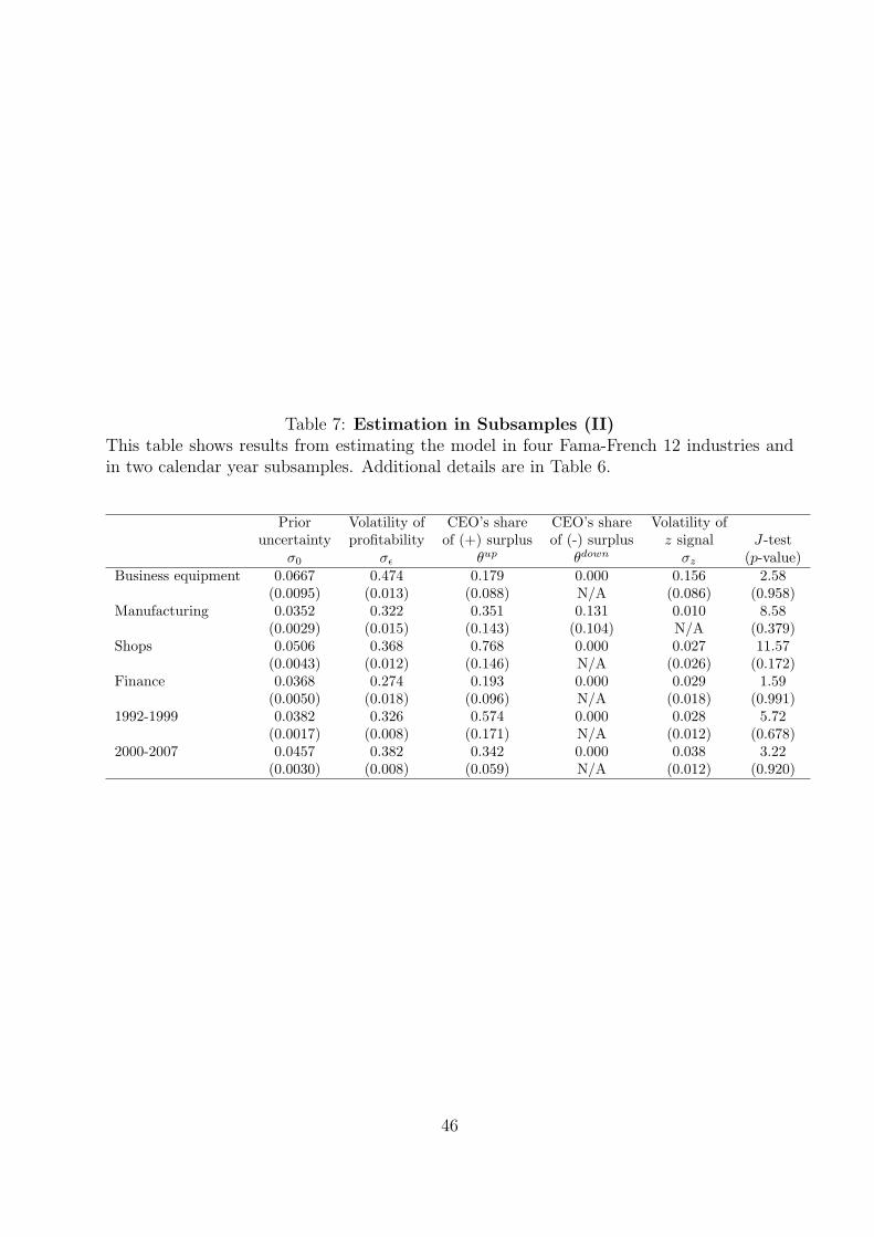
Table 7: Estimation in Subsamples (II)This table shows results from estimating the model in four Fama-French 12 industries andin two calendar year subsamples. Additional details are in Table 6.
Prior Volatility of CEO’s share CEO’s share Volatility ofuncertainty profitability of (+) surplus of (-) surplus z signal J-test
σ0 σϵ θup θdown σz (p-value)Business equipment 0.0667 0.474 0.179 0.000 0.156 2.58
(0.0095) (0.013) (0.088) N/A (0.086) (0.958)Manufacturing 0.0352 0.322 0.351 0.131 0.010 8.58
(0.0029) (0.015) (0.143) (0.104) N/A (0.379)Shops 0.0506 0.368 0.768 0.000 0.027 11.57
(0.0043) (0.012) (0.146) N/A (0.026) (0.172)Finance 0.0368 0.274 0.193 0.000 0.029 1.59
(0.0050) (0.018) (0.096) N/A (0.018) (0.991)1992-1999 0.0382 0.326 0.574 0.000 0.028 5.72
(0.0017) (0.008) (0.171) N/A (0.012) (0.678)2000-2007 0.0457 0.382 0.342 0.000 0.038 3.22
(0.0030) (0.008) (0.059) N/A (0.012) (0.920)
46

Internet Appendix for �CEO Wage Dynamics:Estimates from a Learning Model�
February 10, 2012
Contents
1 Model Solution 1
1.1 Learning and �rst steps . . . . . . . . . . . . . . . . . . . . . . . . . . . . . . 1
1.2 Excess returns . . . . . . . . . . . . . . . . . . . . . . . . . . . . . . . . . . . 2
1.3 Return volatility . . . . . . . . . . . . . . . . . . . . . . . . . . . . . . . . . 5
1.4 CEO pay . . . . . . . . . . . . . . . . . . . . . . . . . . . . . . . . . . . . . . 8
2 Estimating the value of vesting options and restricted stock 9
3 Forecasting Final CEO Tenure Tj 11
4 Details on Cleaning the Data 11
5 Model extension: Endogenous CEO turnover 12
6 Model extension: Learning about �rm quality 15
7 Model extension: Persistent earnings shocks 17
8 CEO Tenure, Return Volatility, and the Variance of Pro�tability 19

1 Model Solution
1.1 Learning and �rst steps
First I solve the learning problem, which is a Kalman �ltering problem. Since prior beliefs
and signals are normally distributed, Bayes�rule tells us that agents�posterior beliefs about
CEO ability will also be normally distributed. At the end of year t; agents�beliefs are
distributed as
�i � N�mit; �
2� it
�; (IA.1)
where � it as the number of years completed by CEO of �rm i as of the end of year t: For
simplicity I drop the subscripts on � : Agents update their beliefs about CEO ability by
observing the mean-zero surprises in pro�tability and the additional signal:
eYit = Yit � ai � vt �mt�1 = �i + "it �mit�1 (IA.2)ezit = zit �mit�1: (IA.3)
Applying Bayes�rule, the posterior variance follows
�2� = �20
�1 + �
��20�2"+�20�2z
���1; (IA.4)
which goes to zero in the limit where tenure � becomes in�nite. The posterior mean belief
mit follows a martingale:
mit = mit�1 +�2��2"eYit+�2�
�2zezit: (IA.5)
Next I solve for the changes in expected pay. From assumption 6, we have
�Et [wit] = �tBit (mit�1 �mit�2) : (IA.6)
Substituting in equation (IA.5) yields
�Et [wit] = �tBit
��2��1�2"
eYit�1+�2��1�2z
ezit�1� : (IA.7)
This equation relates changes in expected compensation to the previous year�s earnings
surprise eYit�1 and additional signal surprise ezit�1:The dividend at the end of year t equals pro�ts minus CEO pay
Dit = BitYit � wit; (IA.8)
1

and the �rm�s value at the beginning of year t equals
Mit = Et
" 1Xs=0
�s+1Dit+s
#: (IA.9)
From this equation I derive the �rm�s stock return, the average industry return (which equals
a constant plus vt), and the stock return in excess of the industry.
1.2 Excess returns
Prediction 1 (excess returns): The excess stock return (�rm minus industry) in year t
equals
rit �BitMit
eYit + BitMit
(1� �t+1) ��1� �T��
1� �
�(mit �mit�1)�median (rit) : (IA.10)
This equation uses the approximation that the pay-performance sensitivity bit is much
less than the �rm�s market value, which I con�rm empirically.
Proof:
First I show that the industry shock to pro�tability, vt; is observable. I adjust pro�tability
and average across the Ni �rms k in �rm i0s industry:
limNi!1
1
Ni
NiXk=1
(Ykt � ak �mkt�1) = vt + limNi!1
1
Ni
NiXk=1
(�k �mkt�1 + "kt) (IA.11)
= vt: (IA.12)
The model assumes agents know or can observe all quantities on the left-hand side, so it
follows that they can also observe the right-hand side, which converges to the industry shock
vt since �k �mkt�1 + "kt has mean zero.
In the remainder of this section I drop the �rm subscript i; for convenience. Also, since
assets Bit are constant over time, I denote them B:
The unexpected stock return is
Rt � Et [Rt] =M�1t (Dt � Et [Dt] +Mt+1 � Et [Mt+1]) (IA.13)
The unexpected dividend is
Dt � Et [Dt] = B (� �mt�1 + vt + "t)� (wt � Et [wt]) (IA.14)
= B�eYt + vt�� btrt; (IA.15)
2

since (as I show later) the expected excess return rt equals zero, implying wt�Et [wt] = btrt.Recalling from the learning results that
mt = mt�1 +�2��2"eYt+�2�
�2zezt (IA.16)
we have
Dt � Et [Dt] = B
��2"�2�(mt �mt�1)�
�2"�2zezt + vt�� btrt: (IA.17)
The surprise in future market value is
Mt+1 � Et [Mt+1] = Et+1 � Et
" 1Xs=0
�s+1Dt+1+s
#(IA.18)
= Et+1 � Et
" 1Xs=0
�s+1 (B� � wit+1+s)#; (IA.19)
because �rm �xed e¤ect ai is known (hence no change in its expected value), and shocks "
and v have conditional mean zero. Combining the results above yields
Rt � Et [Rt] = M�1t
�B�eYt + vt�� btrt� (IA.20)
+M�1t
Et+1 � Et
" 1Xs=1
�s (B� � wit+s)#!
: (IA.21)
The CEO�s last period is T; so there are T � � t+1 periods left at the beginning of periodt + 1. In periods T + 1 and later, a new CEO is in o¢ ce. Before period T; agents learn
nothing about this new CEO�s ability or his expected pay. Therefore we have
Mt+1 � Et [Mt+1] = Et+1 � Et
"T�� t�1Xs=0
�s+1 (B� � wt+1+s)#: (IA.22)
Decomposing into the two pieces and using fact that �rm size and � are constant over time,
Mt+1 � Et [Mt+1] = B (Et+1 � Et [�])T���1Xs=0
�s+1 �T���1Xs=0
�s+1 (Et+1 � Et [wt+1+s])
= B (mit �mit�1) �
�1� �T��
1� �
��T���1Xs=0
�s+1 (Et+1 � Et [wit+1+s]) :
Starting with s = 0; we want to know
Et+1 � Et [wt+1] = Et+1 [wt+1]� Et [Et+1 [wt+1]] : (IA.23)
3

Recall that �t+1 is known at the beginning of period t+1 but not at the beginning of t: We
therefore need to treat �t+1 as a random variable at time t. It is possible to show that
Et+1 � Et [wt+1] = �t+1B (mt �mt�1) + (IA.24)
BEt [mt �mt�1jmt �mt�1 > 0]
��down � �up
2
�:
Using results for the truncated normal distribution, and denoting � (0) the pdf of the stan-
dard normal distribution evaluated at zero, we have
Et+1 � Et [wt+1] = �t+1B (mt �mt�1) +B� (�) : (IA.25)
� (�) � (V art (mijt �mijt�1))1=2� (0)
��down � �up
�:
Using backwards induction, it follows that
Et+1 � Et [wt+1+s] = Et+1 � Et [wt+1] :
Plugging this result in, we have
Mt+1 � Et [Mt+1] = B (mt �mt�1) �
�1� �T��
1� �
�� (Et+1 � Et [wt+1])
T���1Xs=0
�s+1(IA.26)
= �
�1� �T��
1� �
�B [(1� �t+1) (mt �mt�1)� � (�)] ; (IA.27)
and the �rm�s stock return is
Rt = E [Rt] +B
Mt
vt �btMt
rt (IA.28)
+B
Mt
(mt �mt�1)
��2"�2�+ �
�1� �T��
1� �
�(1� �t+1)
�+B
Mt
���
2"
�2z(zt �mt�1)� �
�1� �T��
1� �
�� (�)
�It is possible to show that the average of excess returns rt across industry �rms goes to zero
in the limit as the number of industry �rms becomes in�nite. Since all �rms in the industry
have the same assumed expected return E [R], then the average realized industry return Rtequals
Rt = E [Rt] +
�B
Mt
�vt
4

and the return in excess of the industry return equals1
rt � B
Mt
��2"�2�+ �
�1� �T��
1� �
�(1� �t+1)
�(mt �mt�1) (IA.29)
� BMt
��2"�2z(ezt + � �1� �T��
1� �
�� (�)
�:
We can also write the excess return as
rt � B
Mt
���2"�2�+ �
�1� �T��
1� �
�(1� �t+1)
��2��2"eYt� (IA.30)
+B
Mit
��
�1� �T��
1� �
�(1� �t+1)
�2��2zezt � � �1� �T��
1� �
�� (�)
�=
B
Mt
��1 + �
�1� �T��
1� �
��2��2"(1� �t+1)
� eYt� (IA.31)
+B
Mt
��
�1� �T��
1� �
�(1� �t+1)
�2��2zezt � � �1� �T��
1� �
�� (�)
�(IA.32)
=B
Mt
�eYt + � �1� �T��1� �
�(1� �t+1) (mt �mt�1)� �
�1� �T��
1� �
�� (�)
�:(IA.33)
The various forms of this equation will be useful in various places later in the Appendix.
While eYt and ezt are normally distributed with mean zero, the excess return rt is notnormally distributed, because �t+1 is a binary discrete random variable perfectly correlated
with the sign of eYt �2��2" + ezt �2��2z . The expected excess return is zero, by construction. The
median of eYt �2��2" + ezt �2��2z : is zero, and so is the median of �t+1 �eYt �2��2" + ezt �2��2z� : The medianreturn is therefore
median
�ritj� ; T;
B
Mt
; �; �"; �0; �z; �down; �up
�= � B
Mt
�
�1� �T��
1� �
�� (�) ; (IA.34)
which has the same sign as ���down � �up
�: Substituting this expression into the equations
above yields Prediction 1. End of proof.
1.3 Return volatility
Prediction 2 (excess return volatility):
1Here we use the approximation that the �rm�s time-t book to market ratio, B=Mt; approximately equalsthe industry average ratio, (B=Mt): We also use the approximation bijt << Mit:
5

1. In the special case with no learning, i.e., �20 = 0; or in the limit when tenure goes to
in�nity, then the variance of excess stock returns equals
vart (rit) =
�BitMit
�2�2": (IA.35)
2. In the special case in which �up = �down = 1; meaning the CEO captures the entire
surplus from, then the variance equals
vart (rit) =
�BitMit
�2 ��2��1 + �
2"
�; (IA.36)
where �2��1 is the uncertainty about CEO ability at the beginning of year t, given in
equation (IA.4).
3. If prior uncertainty �20 > 0, the CEO�s share �up = �down = �; and 0 < � < 1, then
the variance of excess stock returns decreases with CEO tenure, increases with prior
uncertainty �0; and decreases with the CEO�s share of the surplus �.
Proof: The proof uses the following result on asymmetric random normal variables. If
X is distributed as N(0; �) and
Y = �+X if X � 0 (IA.37)
= ��X if X < 0; (IA.38)
then the variance of Y equals
V ar (Y ) = �2��2+ + �
2�
2� � (0)2 (�+ � ��)2
�: (IA.39)
I use equation (IA.33) to compute return volatility. Random variable �t+1 depends on
the sign of (mt �mt�1). I introduce notation that will come in handy soon:
�+=� = �
�1� �T��
1� �
�(1� �t+1) (IA.40)
�+ = �
�1� �T��
1� �
�(1� �up) (IA.41)
�� = �
�1� �T��
1� �
�(1� �down); (IA.42)
��T � � ; �up; �down; �
���2+ + �
2�
2� � (0)2 (�+ � ��)2 (IA.43)
6

The variance of the second term in equation (IA.33) is therefore
�B
Mt
�2��4��4�(�2��1 + �
2�) +
�4��4z
��2��1 + �
2z
�+ 2
�4��2��
2z
�2��1
���T � � ; �up; �down; �
�(IA.44)
The variance of the �rst term in equation (IA.33) above is�BitMit
�2 ��2��1 + �
2�
�:
The variance of returns therefore equals
vart (rit) =
�B
Mt
�2 ��2��1 + �
2�
�+ (IA.45)�
B
Mt
�2��4��4�(�2��1 + �
2�)
���T � � ; �up; �down; �
�+�
B
Mt
�2��4��4z
��2��1 + �
2z
�+ 2
�4��2��
2z
�2��1
���T � � ; �up; �down; �
�2B
Mt
�
�1� �T��
1� �
�covt
�~Yt; (1� �t+1) (mt �mt�1)
�:
It is possible to show that the covariance term above equals
covt
�~Yt; �+=� (Zt)
�=�+ + ��2
��2��2�
��2" + �
2��1�+�2��2z�2��1
�;
so return volatility equals
vart (rit) =
�B
Mt
�2 ��2��1 + �
2�
�+ (IA.46)
2
�B
Mt
�2��+ + ��2
��2��2�
��2" + �
2��1�+�2��2z�2��1
��+�
B
Mt
�2��4��4�(�2��1 + �
2�) +
�4��4z
��2��1 + �
2z
�+ 2
�4��2��
2z
�2��1
���T � � ; �up; �down; �
�:
Claim: Holding constant T �� (number of years left in o¢ ce) or setting T �� to in�nity,then we have
lim�!1
vart (rit) =
�BitMt
�2�2": (IA.47)
This results follows by noting
lim�!1
�2��1 = 0: (IA.48)
7

Claim: If �up = �down = �; �20 > 0; and 0 � � � 1; then varit (rit) decreases in tenure.
Proof: Posterior variance �2� is strictly positive and decreasing in � if �20 > 0: The
quantity�1� �T��
�is also decreasing in � : The result follows by inspecting the expression
for return variance, noting that quantities decreasing in � are multiplied by weakly positive
quantities. Even if � = 1; the �rst term in equation (IA.46) still decreases in � :
Claim: If �up = �down = �; and 0 � � � 1; vart (rit) is increasing in �20:
Proof: Posterior variance �2� is increasing in �20: Terms multiplying �� in the expression
above for return variance are all weakly positive, so the conclusion follows.
Claim: If �up = �down = �; �0 > 0; 0 < � < 1; then return variance is strictly decreasing
in �:
Proof: Inspecting the expression for return variance, the term multiplying (1� �) ispositive, so the entire term is strictly decreasing in �:
1.4 CEO pay
Prediction 3 (CEO pay): The change in expected CEO compensation, scaled by the
�rm�s lagged market value, equals
�Et [wit]
Mit�1� rit�1 +
BitMit�1
��2"�2z
�ezit�1 + g (�) (IA.49)
(� ; T ; �; �"; �0; �t) =�2��1�t
�2" + �2��1�
�1��T��+1
1��
�(1� �t)
; (IA.50)
where g is a deterministic function given in the Appendix.
Proof:
Using the last model assumption, we have
�Et [wt]
Mt�1= �t
B
Mt�1(mt�1 �mt�2)
Rearranging equation (IA.29) yields
(mt�1 �mt�2) �rit�1
Mt�1B+ �
�1��T��+1
1��
�� (� � 1)+�2"
�2zezt�1
�2"�2��1
+ ��1��T��+1
1��
�(1� �t)
;
8

so
�Et [wt] � �tBrt�1
Mit�1Bit�1
+ ��1��T��+1
1��
�� (� � 1)+�2"
�2zezijt�1
�2"�2��1
+ ��1��T��+1
1��
�(1� �t)
(IA.51)
�Et [wt]
Mt�1� rt�1 +
B
Mt�1
��2"�2z
�ezt�1 + g (�) (IA.52)
(� ; T ; �; �"; �0; �t) =�2��1�t
�2" + �2��1�
�1��T��+1
1��
�(1� �t)
(IA.53)
g
�� ; T ; �; �"; �0; �t;
B
Mt�1
�=
B
Mt�1� (� � 1) �
�1� �T��+1
1� �
� (:) (IA.54)
Comparative statics for : If there is no learning, i.e., �0 = 0; then = 0 since �2��1 = 0.
Also, in limit where � goes to in�nity then we have �2��1 = 0 and hence = 0: By inspection,
for �0 > 0; slope is increasing in �t; independent of �rm size Mt�1 or B; decreasing
in signal noise �2"; increasing in initial uncertainty �20; and independent of the additional
signal�s precision 1=�z: It is straightforward to show that is decreasing in tenure.
2 Estimating the value of vesting options and restrictedstock
This Appendix explains how I estimate vovestjt; the value of CEO j�s options that vest
during year t; and vsvestt; the value of a CEO shares that vest during year t. The value of
options vesting equals the number of options vesting (novestt) times the price of each option
vesting (pvestt):
vovestt = novestt � povestt: (IA.55)
A similar formula applies to shares vesting:
vsvestt = nsvestt � psvestt: (IA.56)
The number of options vesting during the year is
novestt = opt_unex_exer_numtajextajext�1
� opt_unex_exer_numt�1 + opt_exer_numt:
(IA.57)
opt_unex_exer_numt is Execucomp�s number of unexercised exercisable options held by
the CEO at the end of �scal year t: The ratio ajext=ajext�1 (also Execucomp variables)
adjusts for stock splits during year t: opt_exer_numt is Execucomp�s number of shares
obtained upon exercising options during year t: The explanation for the formula above is
9

that the CEO starts year t with a supply of options opt_unex_exer_numt�1 that have
already vested but have not yet been exercised. An amount novestjt of new options vests,
then the CEO gets rid of some of these options by exercising them (opt_exer_numt), so
the CEO is left with a supply opt_unex_exer_numt of vested but unexercised options at
the end of year t: The formula assumes that options are exercised before any stock splits
occur. I set novest equal to zero for fewer than 5% of observations that are negative.
The number of shares vesting during the year is given by
nsvestt = stock_unvest_numt�1 � stock_unvest_numtajextajext�1
+ new_granted_numt
(IA.58)
stock_unvest_numt is Execucomp�s number of shares of restricted stock held by the ex-
ecutive that had not yet vested by the end of year t: new_granted_numt is the num-
ber of new shares of restricted stock granted during the year, which I estimate by divid-
ing the dollar value of newly granted options (Execucomp variable rstkgrntt before 2006,
stock_awards_fvt in 2006 and later) by St; the midpoint of the starting and ending share
price for the year. To understand the formula for nsvestt, the CEO starts with a supply
of unvested shares at the beginning of the year (stock_unvest_numt�1), then he or she
receives some new shares (new_granted_numt); then nsvestt shares vest, so the CEO is
left with a supply stock_unvest_numt of unvested shares at the end of the year. I set
nsvestt to zero if it takes a negative value. Since I do not know the exact date when the
shares vest, I assume they vest at a share price psvestt midway between the starting and
ending price for the year.
I estimate the price of the vesting options using the Black-Scholes formula, adjusted for
dividends. I estimate the strike price Kt�1 for vesting options using the method of Core
and Guay (2002), as described in Edmans, Gabaix, and Landier (2009):
Kt�1 = St �opt_unex_exer_est_valt�1opt_unex_exer_numt�1
: (IA.59)
opt_unex_exer_est_valt�1 is the Execucomp estimated value of unexercised exercisable
options at the end of �scal year t � 1: The dividend rate is Execucomp variable bs_yieldmeasured at end of �scal year t; divided by 100: I impute a zero if this variable is missing.
I also winzorize this variable at the 95th percentile each year. Black-Scholes volatility is
given by Execucomp variable bs_volatility at end of �scal year t: If this variable is missing,
I replace it with the year�s median value. I winzorize volatility at the 5th and 95th percentile
each year. The risk free rate is the continuously compounded risk-free rate, derived from
the one-month Treasury rate in July of year t: Following the method of Core and Guay
10

(2002) and Edmans, Gabaix, and Landier (2008), I set the average maturity of maturing
options equal to the maturity of options granted during year t (computed using Execucomp
option maturity date, exdate); minus four years. If there were no new grants in year t then
I set Tt = 5:5 years. In the case of multiple new grants during year t; I take the longest
maturity option. If maturity becomes negative then I set maturity equal to 1 day.
3 Forecasting Final CEO Tenure Tj
This section explains how I forecast Tj (the total number of years CEO j spends in o¢ ce)
for CEOs who have not left o¢ ce by the end of the sample period. Forecasted Tj equals the
CEO�s tenure in his last record in Execucomp plus the forecasted number of years left in
o¢ ce, denoted Y earsLeftjt. The forecast is based on the following regression:
log (1 + Y earsLeftjt) = log a0 + b1 logAgejt + b2 log Tenurejt + "jt: (IA.60)
Agejt is CEO j�s age in year t (Execucomp variable AGE): I estimate the regression by
taking CEOs whose last year in o¢ ce is in the database, and then creating one regression
observation for each year the CEO spent in o¢ ce, potentially including years before 1992.
The regression uses 14,111 observations and has an R2 value of 0.23. Forecasted Tj is then
bTj = Tenurejt� + ba0Agebb1jt�Tenurebb2jt� � 1 (IA.61)
= Tenurejt� + e12:5Age�2:75jt� Tenure0:114jt� � 1; (IA.62)
where t� denotes CEO j�s last year in the database. bTj is missing if Agejt or Tenurejt ismissing.
4 Details on Cleaning the Data
I clean the data as follows. First I �ll in missing CEO indicators in Execucomp. I label an
individual to be CEO in a �rm/year observation if (i) Execucomp lists no one as CEO in
the given �rm/year, and (ii) either (a) this individual was CEO of the �rm in previous and
following year; (b) this individual was CEO in previous year, and we don�t know who was
CEO in following year; or (c) this person was CEO in following year, and we don�t know
who was CEO in previous year. I assume the CEO�s �rst �scal year is the one when he
completes at least 6 full months in o¢ ce. I use Execucomp variable BECAMECEO as the
date the CEO started in o¢ ce. I exclude observations where BECAMECEO is missing.
11

Next I exclude all observations for those CEOs whose start date (BECAMECEO) is more
than one year after their �rst yearly record as CEO in Execucomp; I assume these are data
mistakes in Execucomp. Next I exclude �rm/year observations where the CEO�s �rst �scal
year in o¢ ce is less than 6 months long; I keep these CEOs�later years in o¢ ce. I cannot
compute the vesting compensation measure in the CEO�s �rst year in Execucomp, because
computing the value of shares and options vesting in year t requires Execucomp data from
year t� 1: Therefore, I cannot compute the change in this pay measure in a CEO�s �rst twoyears in Execucomp. In years when change in pay is missing for mechanical reasons, I keep
the years�stock return observation but treat the change in pay variable as missing. For
other years, I delete �rm/year records where change in pay is missing. I exclude �rm/years
where I cannot observe or forecast the CEO�s total tenure Tj: Next I exclude �rm/years
where I cannot �nd the �rm�s lagged market cap in CRSP, and then I eliminate �rm/years
in which the variance of excess returns is missing.
5 Model extension: Endogenous CEO turnover
This robustness section extends the model to allow endogenous CEO turnover and then
estimates the extended model. The extended model is similar to Taylor (2010). All the
assumptions are the same as in the original model, but now we assume the board chooses
whether or not to �re the CEO at the beginning of each year. Firing the CEO costs the
�rm a fraction c of its assets. The board�s goal is to maximize �rm value.
The �rm�s dividend is now
Dit = Yit � 1 (fireit)Bic� wit (IA.63)
where 1 (fireit) is an indicator equal to 1 if the �rm �res the CEO at the end of year t: The
board makes CEO �ring decisions that maximize �rm value.
The board�s optimization problem is
maxffireit+sg1s=0
Mt; (IA.64)
where Mt is the �rm�s market value at the beginning of year t; before the �ring decision has
12

been made.We therefore have
M�t = max
ffireit+sg1s=0Et
" 1Xs=0
�s+1Dit+s
#(IA.65)
= maxffireit+sg1s=0
Et
" 1Xs=0
�s+1 (BiYit+s � 1 (fireit+s)Bic� wit+s)#
(IA.66)
= maxffireit+sg1s=0
Et
" 1Xs=0
�s+1 (Bi (ai + �i)� 1 (fireit+s)Bic� wit+s)#; (IA.67)
since shocks vt and "it have mean zero. We therefore have
M�t
Bt= ai
�
1� � + maxffireit+sg1s=0
Et
" 1Xs=0
�s+1��i � 1 (fireit+s) c�
wit+sBi
�#(IA.68)
= ai�
1� � + maxffireit+sg1s=0
Et
" 1Xs=0
�s+1�mit�1+s � 1 (fireit+s) c�
Et+s [wit+s]
Bi
�#(IA.69)
I de�ne �t as the di¤erence between posterior and the prior belief:
mit = mi0 +�it: (IA.70)
Also, I denote initial expected pay when the CEO enters o¢ ce E [w0] : Substituting in yields
M�t
Bt= (ai +mi0 � E [wi0])
�
1� � + (IA.71)
maxffireit+sg1s=0
Et
" 1Xs=0
�s+1��it�1+s � 1 (fireit+s) c�
Et+s [wit+s]� E [w0]Bi
�#M�t
Bt= (ai +mi0 � E [wi0])
�
1� � + V�t (IA.72)
where V �t is the value function:
V �t = �maxfireit
��it�1 �
Et [wit]� E [w0]Bi
� 1 (fireit) c�+ �Et
�V �t+1
�: (IA.73)
The state variable is
xit � �it�1 �Et [wit]� E [w0]
Bi; (IA.74)
which equals zero when the CEO �rst starts in o¢ ce. State variable x equals the cumulative
CEO surplus captured by the shareholders, plus a constant. We know the dynamics for �it
and Et [wit] :
�it = �it�1 + (mit �mit�1) (IA.75)Et+1 [wit+1]
Bi=
Et [wit�1]
Bi+ �t+1 (mit �mit�1) (IA.76)
13

so
xit+1 = xit + (mit �mit�1) (1� �t+1) ; (IA.77)
where
mit �mit�1 � N�0; �2��1�
2�
�1
�2"+1
�2z
��(IA.78)
by Bayes�Rule. Since the dynamics of x depend on tenure � ; � is also a state variable. I
therefore write V � as a function: V � (x; �) : If the board �res its CEO, it hires a new one so
that the value function resets to
Vfire = V (x = 0; � = 1)� c: (IA.79)
If the CEO retires voluntarily, then the value function resets to
Vret = V (x = 0; � = 1) : (IA.80)
CEOs voluntarily retire after tenure year � with probability pret (�) ; estimated using data
on voluntary successions as in Taylor (2010). If the �rm chooses not to �re its CEO, then
Vkeep = �xit + �Et�V �t+1
�(IA.81)
= �xit + � (pretVret + (1� pret)Et [V (xit+1; � + 1)]) : (IA.82)
The �rm chooses whether to �re the CEO at time t according to
V (xit; � t)� = max fVfire; Vkeepg (IA.83)
= maxfV (0; 1)� c; (IA.84)
�xit + � (pretVret + (1� pret)Et [V (xit+1; � + 1)])g: (IA.85)
Collecting results, the �rm�s market value equals
M�it
Bi= k + V � (xit; � it) (IA.86)
k � (ai +mi0 � E [wi0])�
1� � (IA.87)
V � (xit; � it) = maxfV (0; 1)� c; (IA.88)
�xit + � (pret (�)V (0; 1) + (1� pret (�))Et [V (xit+1; � + 1)])g(IA.89)Vret = V � (0; 1) (IA.90)
xit+1 = xit + (mit �mit�1) (1� �t+1) (IA.91)
mit �mit�1 � N
�0; �2��1�
2�
�1
�2"+1
�2z
��(IA.92)
�t+1 = �up if mit �mit�1 > 0; otherwise �t+1 = �down: (IA.93)
14

In simulations I choose k so that the simulated market-to-book ratio equals its empirical
counterpart.
I simulate returns using the following equations:
Rit =Dit +Mit+1
Mit
� 1 (IA.94)
=Yit � Et [wijt] =B � brit=B +Mit+1=B
Mit=B� 1 (IA.95)
� Yit � Et [wijt] =B + k + V (xt+1; � + 1)k + V (xt; �)
� 1: (IA.96)
Unexpected returns equal
rit = Rit � Et [Rit] (IA.97)
=eYit + V (xt+1; � + 1)� E [V (xt+1; � + 1)jxt; � ]
k + V (xt; �): (IA.98)
6 Model extension: Learning about �rm quality
I make the following changes in notation. For convenience I drop subscripts on several
variables. batjs and b�js denotes the posterior mean of ait and �i; respectively, at the end ofperiod s: Therefore, b�js = mis from the original notation. �atjs and ��js are the posterior
variance of beliefs about ait and �i; respectively, at the end of period s: I drop �rm subscripts
i for convenience.
I write the problem in vector form to apply the multivariate version of Bayes�rule. State
variable xt ��at �
�0follows (as long as CEO stays in o¢ ce)
xt = �xt�1 + (I � �)�a0
�+
�ut0
�(IA.99)
� =
�� 00 1
�: (IA.100)
Beliefs about xt at the end of period t � 1 are distributed as N��tjt�1;tjt�1
�; and beliefs
about xt at end of period t are distributed as N��tjt;tjt
�: From the law of motion for x we
15

can immediately write
�tjt�1 = ��t�1jt�1 + (I � �)�a0
�(IA.101)
tjt�1 = �0t�1jt�1� +
��2u 00 0
�: (IA.102)
When a new CEO takes o¢ ce at the beginning of period t we set the o¤-diagonal elements of
tjt�1 to zero and the diagonal element corresponding to � to �20; meaning that uncertainty
about the CEO resets to the prior uncertainty while uncertainty about �rm quality keeps its
current value: The signal observed each period is
Xt ��Yt � vtzt
�= �xt + "t (IA.103)
� =
�1 10 1
�; "t =
�"t�zt
�� N (0;�) (IA.104)
� =
��2" 00 �2z
�: (IA.105)
Bayes rule states that
�tjt = tjt
��1tjt�1�tjt�1 +�
0��1Xt
�: (IA.106)
tjt =h�1tjt�1 +�
0��1�i�1
: (IA.107)
Next I provide an expression for excess stock returns. In the original model, excess
returns are given in equation (nref{eq_r_ztilde}). The only di¤erence in this model is
that the �rm�s market value moves due to changes in beliefs about at; �rm quality. The
contribution of �rm quality to market value at the beginning of period t is
B�1Xs=0
�sEt [at+s] : (IA.108)
It is straightforward to show that
Et [at+s] = �s+1bat�1jt�1 + a �1� �s+1� ; (IA.109)
hence
B�
1Xs=0
�sEt [at+s] = B�
1Xs=0
�s��s+1bat�1jt�1 + a �1� �s+1�� (IA.110)
= B�
1Xs=0
�s��s+1
�bat�1jt�1 � a�+ a� (IA.111)
16
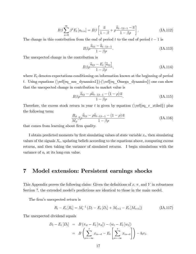
B�
1Xs=0
�sEt [at+s] = B�
�a
1� � + �bat�1jt�1 � a1� ��
�: (IA.112)
The change in this contribution from the end of period t to the end of period t� 1 is
B��batjt � bat�1jt�11� �� : (IA.113)
The unexpected change in the contribution is
B��batjt � Et �batjt�1� �� ; (IA.114)
where Et denotes expectations conditioning on information known at the beginning of period
t: Using equations (nref{eq_mu_dynamics1})-(nref{eq_Omega_dynamics}) one can showthat the unexpected change in contribution to market value is
B��batjt � �bat�1jt�1 � (1� �) a
1� �� : (IA.115)
Therefore, the excess stock return in year t is given by equation (nref{eq_r_ztiled}) plusthe following term:
BitMit
��batjt � �bat�1jt�1 � (1� �) a
1� �� (IA.116)
that comes from learning about �rm quality.
I obtain predicted moments by �rst simulating values of state variable xt; then simulating
values of the signals Xt; updating beliefs according to the equations above, computing excess
returns, and then taking the variance of simulated returns. I begin simulations with the
variance of at at its long-run value.
7 Model extension: Persistent earnings shocks
This Appendix proves the following claim: Given the de�nitions of x; �; and Y in robustness
Section ?, the extended model�s predictions are identical to those in the main model.
The �rm�s unexpected return is
Rt � Et [Rt] =M�1t (Dt � Et [Dt] +Mt+1 � Et [Mt+1]) (IA.117)
The unexpected dividend equals
Dt � Et [Dt] = B (�it � Et [�it])� (wt � Et [wt])
= B
tX
s=�1xis!t � Et
"tX
s=�1xis!t
#!� btrt:
17
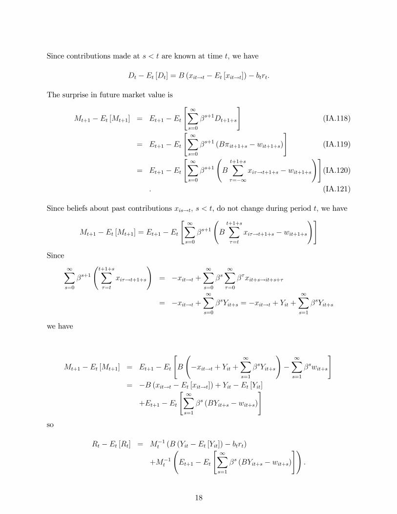
Since contributions made at s < t are known at time t; we have
Dt � Et [Dt] = B (xit!t � Et [xit!t])� btrt:
The surprise in future market value is
Mt+1 � Et [Mt+1] = Et+1 � Et
" 1Xs=0
�s+1Dt+1+s
#(IA.118)
= Et+1 � Et
" 1Xs=0
�s+1 (B�it+1+s � wit+1+s)#
(IA.119)
= Et+1 � Et
" 1Xs=0
�s+1
B
t+1+sX�=�1
xi�!t+1+s � wit+1+s
!#(IA.120)
: (IA.121)
Since beliefs about past contributions xis!t; s < t, do not change during period t; we have
Mt+1 � Et [Mt+1] = Et+1 � Et
" 1Xs=0
�s+1
Bt+1+sX�=t
xi�!t+1+s � wit+1+s
!#
Since
1Xs=0
�s+1
t+1+sX�=t
xi�!t+1+s
!= �xit!t +
1Xs=0
�s1X�=0
��xit+s!it+s+�
= �xit!t +1Xs=0
�sYit+s = �xit!t + Yit +1Xs=1
�sYit+s
we have
Mt+1 � Et [Mt+1] = Et+1 � Et
"B
�xit!t + Yit +
1Xs=1
�sYit+s
!�
1Xs=1
�swit+s
#= �B (xit!t � Et [xit!t]) + Yit � Et [Yit]
+Et+1 � Et
" 1Xs=1
�s (BYit+s � wit+s)#
so
Rt � Et [Rt] = M�1t (B (Yit � Et [Yit])� btrt)
+M�1t
Et+1 � Et
" 1Xs=1
�s (BYit+s � wit+s)#!
:
18

Substituting in equation (1), the assumption that the �rm �xed e¤ect is known, and the
industry shock is i.i.d. with mean zero, we have
Rt � Et [Rt] = M�1t
�B�eYt + vt�� btrt�
+M�1t
Et+1 � Et
" 1Xs=1
�s (B� � wit+s)#!
:
This equation is identical to equation nref{eq_app_connect_exvol} in Appendix ??, so thepredictions about excess returns will be identical as in the main model. Since the equation
for Yit has not changed, the equations for learning dynamics will not change, and neither
will the equations for wage dynamics.
8 CEO Tenure, Return Volatility, and the Variance ofPro�tability
Figure 2 in the main paper shows that excess stock return volatility declines after a new
CEO takes o¢ ce. The model attributes this decline to learning about CEO ability. In this
section I test an alternate explanation, which is that earnings volatility declines with CEO
tenure. First I estimate the shocks to pro�tability, then I check whether the volatility of
these shocks changes with CEO tenure. For comparison, I con�rm that return volatility
declines with tenure even after including additional controls.
I compute annual return on assets (ROA) for every �rm/year in the sample. I estimate
earnings shocks "it using the following panel model:
ROAit = �0 + �1ROAit�1 + �2 log (Assetsit�1) + �i + �t + �� + "it; (IA.122)
where �i is a �rm �xed e¤ect, �t is a year �xed e¤ect, and �� is a CEO tenure �xed e¤ect
for tenure categories � = 1; :::; 10+ years. The conditional mean of the squared residuals,
E ["2itjregressors] ; equals the conditional variance of pro�tability. I estimate this conditionalvariance from the following regression:
b"2it = 0 + 1 log (Assetsit�1) + i + t + � + uit; (IA.123)
where b"2it is estimated from regression (IA.122), i is a �rm �xed e¤ect, t is a year �xed
e¤ect, and � is a CEO tenure �xed e¤ect.
Table 1 shows the estimated tenure �xed e¤ects � for the conditional variance of ROA:
The �xed e¤ect for tenure = 10+ years is normalized to zero. None of the tenure �xed
19

e¤ects is sign�cantly di¤erent from zero. The conditional variance of pro�tability shows no
signi�cant pattern with CEO tenure.
For comparison, I measure tenure �xed e¤ects in excess return volatility. I regress
RETVAR (the annualized variance of excess stock returns) on log lag assets, �rm �xed
e¤ects, year �xed e¤ects, tenure �xed e¤ects, and (in one speci�cation) the squared shocks
to ROA (b"2it). Results are in Table 1. The �xed e¤ect for tenure equal one (two) years
is signi�cantly positive at the one (ten) percent con�dence level, and the remaining �xed
e¤ects are indistinguishable from zero, consistent with the result in Figure 3. In sum, return
volatility declines signi�cantly with tenure, but earnings volatility does not.
20

Table 1: CEO Tenure, Return Volatility, and the Variance of Pro�tabilityThis table shows the variance of �rm pro�tability and excess stock returns, conditional onCEO tenure and other controls. The variance for CEOs with tenure = 10+ is normalizedto zero. First I estimate shocks to return on assets (ROA) by regressing ROA on its lag,log(lag assets), �rm �xed e¤ects, year �xed e¤ects, and CEO tenure �xed e¤ects (results notshown). I then square the estimated residuals and regress these on log lag assets, �rm �xede¤ects, year �xed e¤ects, and tenure �xed e¤ects; estimates are below. The table also showsthe tenure �xed e¤ects from a regression of RETVAR (annualized variance of excess stockreturns) on log lag assets, �rm �xed e¤ects, year �xed e¤ects, tenure �xed e¤ects, and thesquared shock to ROA. The sample contains is described in section IV.B. Standard errorsare in parentheses.
Dependent variableSquared ROA Variance of excess Variance of excess
CEO tenure (yrs) shock returns returns1 0.0009 0.0264 0.0263
(0.0031) (0.0033) (0.0033)2 0.0025 0.0060 0.0050
(0.0032) (0.0034) (0.0034)3 0.0009 0.0034 0.0033
(0.0033) (0.0035) (0.0035)4 -0.0012 0.0027 0.0029
(0.0034) (0.0036) (0.0036)5 0.0001 -0.0001 -0.0004
(0.0035) (0.0037) (0.0037)6 -0.0015 0.0038 0.0038
(0.0036) (0.0038) (0.0038)7 -0.0024 -0.0003 -0.0007
(0.0038) (0.0040) (0.0040)8 -0.0027 -0.0017 -0.0014
(0.0039) (0.0041) (0.0041)9 -0.0028 -0.0025 -0.0022
(0.0040) (0.0043) (0.0043)10+ 0 0 0
N/A N/A N/Alog(lag assets) 0.0044 -0.0189 -0.0183
(0.0018) (0.0019) (0.0019)Squared ROA 0.0584
shock (0.0079)Year �xed e¤ects Yes Yes YesFirm �xed e¤ects Yes Yes Yes
N 20,400 20,482 20,400R-squared 0.183 0.612 0.614
21