Embed Size (px)
Citation preview

ON THE USE OF HONESTY PRIMING TASK TO MITIGATE HYPOTHETICAL BIAS IN CHOICE EXPERIMENTS
DE MAGISTRIS, T. GRACIA, A. NAYGA, R.M. Jr.
Documento de Trabajo 12/01
CENTRO DE INVESTIGACIÓN Y TECNOLOGÍA AGROALIMENTARIA DE ARAGÓN (CITA)
UNIDAD DE ECONOMÍA AGROALIMENTARIA Y DE LOS RECURSOS NATURALES Avda. Montañana, 930 Teléfono: 976716305 50059 ZARAGOZA Fax: 976716335

1
On the use of honesty priming task to mitigate hypothetical bias in choice
experiments
Tiziana de- Magistris*, Azucena Gracia**, Rodolfo M. Nayga, Jr.***
*Tiziana de Magistris is Researcher Outgoing Marie Curie at the Unidad de Economía
Agroalimentaria y de los Recursos Naturales. Centro de Investigación y Tecnología
Agroalimentaria de Aragón (CITA), Gobierno de Aragón. Zaragoza (Spain). email:
[email protected] (Corresponding author)
**Azucena Gracia is Senior Researcher at the Unidad de Economía Agroalimentaria y
de los Recursos Naturales. Centro de Investigación y Tecnología Agroalimentaria de
Aragón (CITA), Gobierno de Aragón. Zaragoza (Spain).
***Rodolfo M. Nayga, Jr. is Professor and Tyson Endowed Chair at the Department of
Agricultural Economics and Agribusiness, University of Arkansas, Fayetteville, AR,
USA.
Corresponding author: Tiziana de Magistris, email: [email protected]
2
Abstract
We test whether the use of an honesty priming task from the social psychology
literature can help mitigate hypothetical bias in stated preference choice experiments
(CE). Using a between-sample design, we conducted experiments with five treatments:
(1) hypothetical CE without cognitive task, (2) hypothetical CE with cheap talk script,
(3) hypothetical CE with neutral priming task, (4) hypothetical CE with honesty priming
task, and (5) non-hypothetical CE. Results generally suggest that marginal willingness
to pay estimates from treatment 4 where subjects are given honesty priming task before
the choice experiment are not statistically different from marginal valuations from
treatment 5 where subjects are in a non-hypothetical choice experiment. Values from
both these treatments are significantly lower than those from other three hypothetical
treatments (treatments 1-3). Using hold out tasks, our results also suggest that one
could get higher percentage of correct predictions of participants’ choices in treatments
4 and 5 than in treatments 1-3 and that there is no significant difference in percentage of
correct predictions between treatments 4 and 5.
Keywords: hypothetical bias, cheap talk, priming, Willingness-to-pay
JEL Classification: C23, D12, Q18
We are thankful for funding from FOODLABELS_PIOF-GA-2009-253323
The authors thank Jayson Lusk, Min Ding, Dirk Smeesters, and Faical Akaichi for helpful
comments
3
Eliciting people’s preferences for various goods using stated preference methods
is a common practise in the applied economics and the marketing literature. In
particular, the choice experiment (CE) approach is now the most widely used stated
preference method in valuing products or attributes. There are literally hundreds of
studies published in the literature of various disciplines that have used choice
experiments. Some of the reasons for CE’s popularity include its flexibility to take
into account several attributes which can be estimated simultaneously and its
consistency with random utility theory and Lancaster’s consumer theory. Individual
CE questions are also framed in a manner that closely resembles consumer shopping
situations (Lusk and Schroeder, 2004).
Hypothetical bias, however, still represents a challenging issue in stated
preference CE studies. It is well known that hypothetical bias occurs when individuals
overstate their willingness- to- pay (WTP) in hypothetical settings due to among
others, lack of economic incentive to reveal their true valuations (List and Gallet,
2001; Murphy et al., 2005; Hensher, 2010). List and Gallet (2001) conducted a meta-
analysis of 29 experimental studies which revealed that subjects on average overstate
their preferences by a factor of 3 in hypothetical settings. They also reported that the
hypothetical bias was considerably less for private goods compared to public goods.
In the same token, Murphy et al. (2005) also carried out a meta-analysis of 28 studies
and reinforced the findings of List and Gallet (2001) by showing that the mean ratio
of hypothetical to actual values is around 1.35 and that the bias increased when public
goods were valued.
Research related to hypothetical bias can be split into two groups. The first group
is focused on the introduction of incentive compatible mechanisms to obtain more

4
realistic value estimates in CEs. These studies test hypothetical bias by comparing
hypothetical WTPs with non-hypothetical WTPs from these incentive compatible
CEs. The second group of papers, while not necessarily utilizing CE, works in the
development of various techniques for mitigating the hypothetical bias.
The findings of the few papers belonging to the first group mentioned above
have been mixed. For instance, while Carlsson and Martinsson (2001) and Cameron et
al. (2002) failed to reject the hypothesis that marginal WTPs from both hypothetical
and non-hypothetical CEs are equal, other studies such as Johansson-Stenman and
Svedsater (2008) and Loomis et al., (2009) have found substantial hypothetical bias in
hypothetical CE markets. Lusk and Schroeder (2004) also showed that total WTPs in
hypothetical CE were different from WTPs in non-hypothetical CE for a private good.
However, they were not able to find the same result with the marginal WTPs. Finally.
Chang et al. (2009) also found that the non-hypothetical choices are a better
approximation of true preferences than hypothetical choices based on a comparison of
hypothetical and non-hypothetical CEs as well as comparison of predicted market
shares from these experiments with actual market shares.
In the second group of studies, the seminal paper by Cummings and Taylor (1999)
introduced a cheap talk script which explained the problem of hypothetical bias to
participants prior to administration of the valuation questions. The authors found that
the cheap talk script was effective in removing the hypothetical bias with public
goods. Carlsson et al. (2005) also confirmed that cheap talk script decreased the WTP
in hypothetical settings. Several other studies, however, have found that there is
heterogeneity on the effects of cheap talk. For example, List (2001) used a cheap talk
for private goods in a field experiment and concluded that experienced card dealers
did not change their WTPs based on cheap talk scripts. However, the cheap talk was

5
able to eliminate the hypothetical bias for inexperienced consumers. Consistent with
List (2001), Lusk (2003) found that cheap talk did not reduce WTP values of
knowledgeable consumers. He also reported that estimated WTP calculated from
hypothetical responses with cheap talk was not significantly lower than willingness to
pay estimates from hypothetical responses without cheap talk. Moreover, Brummett,
Nayga and Wu (2007) pointed out that their cheap talk script was not able to remove
the hypothetical bias because there were no differences in their WTP estimates with
and without cheap talk. On the other hand, Tonsor and Shupp (2011) reported that
cheap talk provided in CEs conducted online can reduce the absolute value of mean
WTP while Silva et al. (2011) found that their cheap talk eliminated the hypothetical
bias in a retail setting.
Taking into account the mixed evidence on the ability of the cheap talk technique
to mitigate hypothetical bias in stated preference studies, we propose and test a new
type of ex-ante calibration method taken from the social psychology literature: a
honesty priming technique. In particular, we test whether exposure to honesty
concepts could unconsciously activate honesty among subjects so that they can
respond truthfully and in turn mitigate potential hypothetical bias in hypothetical CEs.
This is the main contribution of our paper.
Psychologists call the technique that implicitly stimulates certain behaviors as
unconscious “priming”. Psychologists have found that stereotyping behavior can be
stimulated by priming a social category. Priming is conceptually related to the
underlying psychological processes used to activate mental representations in a
passive, unintended, and unconscious way. Recently, several studies in social
cognition and psychology research have demonstrated that “priming” can
unconsciously influence peoples’ perception, evaluations, behavior and choice
6
(Maxwell, Nye, and Maxwell, 1999; Bargh et al., 2001; Kay and Ross, 2003;
Chartrand et al., 2008). In other words, when people are incidentally exposed to some
cues or words in an unrelated subsequent choice task, these stimuli can activate
different buying goals, thereby influencing their subsequent decision in a non-
conscious manner (Chartrand et al., 2008). For example, Maxwell, Nye, and Maxwell
(1999) demonstrated that participants who were primed for fairness showed more
cooperative behavior and, consequently, had a more positive attitude towards the
seller. Hence, the sellers could increase a buyers’ satisfaction without sacrificing
profit. Bargh et al. (2001) also pointed out that when participants were primed with
the concept of automatic achievement, the goal to better perform was activated
without their awareness in an unrelated subsequent task. In the same line, Kay and
Ross (2003) exposed people to some words related to either cooperation or
competition in order to demonstrate that a link between priming and deliberative
behavior exists. Their findings showed a high correlation between people given the
cooperative and competitive priming condition and their deliberative intention to
cooperate and compete, respectively.
With the use of an honesty priming task, our premise in this paper is that among
others, untruthful choice revelations is one of the major causes of hypothetical bias in
stated preference CEs. To test the effectiveness of the honesty priming technique in
reducing hypothetical bias in CE, we conducted an experiment with five treatments:
(1) a hypothetical CE, (2) a hypothetical CE with cheap talk, (3) a hypothetical CE
with neutral priming, (4) a hypothetical CE with honesty priming, and (5) non-
hypothetical CE. The introduction of the five treatments allows us not only to test if
the honesty priming technique can mitigate hypothetical bias in hypothetical settings
but also to test if this priming task can mitigate the hypothetical bias more than the
7
use of cheap talk script and if their marginal WTPs are lower or similar than those
from a non-hypothetical CE. Results from the different tests may open new avenues in
stated preference research and have implications on the use of incentive compatible
elicitation mechanisms in choice experiments.
The rest of the article is organized as follows: the next section discusses the
experimental design and explains the rationale for inclusion of these treatments. The
section following this describes the results and the final section discusses the
importance and the implications of these findings for use of hypothetical and non-
hypothetical CE in future studies.
Experimental Design
General design and treatments’ description
The experiment was conducted in the region of Aragón (Spain), in the town of
Zaragoza during September-October 2011. In our experiment we randomly recruited
participants in different locations across the city using a sampling procedure (by age,
gender and education level). Target respondents were the primary food buyers in the
household and only households who consumed our product of interest were finally
included in the sample. In total, 265 participants were recruited and they were
randomly allocated to the different treatments in our experiment. In accordance with
Lusk and Schoeder (2004), we followed a between-subject approach where each
respondent participates only in one of the treatments. The random assignment has
successfully provided us with similar socio-demographic profiles of subjects across
the treatments.
8
To investigate our main objective, the first four treatments are in hypothetical
settings while the fifth treatment utilizes an incentive aligned elicitation mechanism.
In the first treatment (T1), we used a hypothetical choice experiment without any
cognitive task. In the second one, we introduced a generic and short cheap talk script
before participants responded to the CE questions. We refer to this as our cheap talk
treatment (CT). In the third and fourth treatments, called neutral priming treatment
(NP) and honesty priming treatment (HP), respectively, we used a subliminal priming
technique (before presentation of the CE questions) called “scrambled sentence test”
where participants were asked to construct 24 grammatically correct sentences out of
a series of words presented in a scrambled order. The difference between the neutral
and the honesty tasks is that while in the honesty task the final sentences are related to
honesty, fairness and truthfulness (16 out of 24), in the neutral task, all the final
sentences are not related to any of honesty concepts but rather on just general and
highly known topics (e.g., earth is round, summer is hot). We use the neutral priming
task in addition to the honesty priming task to ensure that we could test and know that
the priming did not arise purely due to the nature of the scrambling task but rather due
to the activation of honesty concepts. Finally, the fifth treatment (T5) is similar to the
first treatment (T1) but with the addition of an incentive aligned elicitation
mechanism to make the CE non-hypothetical. We used treatment 1 (T1) and treatment
5 (T5) as our baseline treatments given that the participants in these treatments were
not exposed to any cognitive task (i.e., cheap talk, neutral priming or honesty priming)
prior to the conduct of the choice experiment. The information is shown in Annex 1.
To test if our proposed honesty priming task mitigates the hypothetical bias in
hypothetical setting and to test if it can be more effective than the traditional cheap
talk script, we test the following null hypotheses:

9
H01= (WTPT1 -WTP
T5)=0
H11= (WTP
T1-WTP
T5 )>0
H02= (WTP
NP – WTP
HP)=0 H12= (WTP
NP-WTP
HP )>0
H03= (WTPT1 – WTP
HP)=0 H13= (WTP
T1-WTP
HP )>0
H04= (WTPCT – WTP
HP)=0 H14= (WTP
CT-WTP
HP )>0
where WTP are the estimated marginal willingness to pay1.
If we reject H01 we can confirm that hypothetical bias exists in hypothetical
choice experiments. If H02 is rejected, we can conclude that the neutral priming task
does not change the marginal WTPs and therefore, ensures that priming effects do not
arise purely due to the nature of the sentence scrambling task but rather due to the
activation of honesty concepts. If H03 is rejected, we can conclude that the honesty
priming task indeed reduces the hypothetical bias in hypothetical setting. Finally, if
H04 is rejected, we can confirm that the honesty priming task reduces the hypothetical
bias to a larger extent than the cheap talk script. Overall, if we reject all the above
hypotheses we may conclude that hypothetical bias indeed exists in hypothetical
choice experiments and that the use of the honesty priming task can reduce the
hypothetical bias in hypothetical choice experiment and, the reduction is larger than
the one achieved by the cheap talk script.
To further test the robustness of our results, we test also the following hypothesis:
H05= (WTPNP – WTP
T1 )=0
H15= (WTP
NP-WT
T1 )#0
If H05 is rejected (once H02 had been also rejected), this would mean that the
WTPs from the neutral priming treatment are different from the WTPs from the
10
baseline hypothetical choice experiment treatment (T1) and this difference in WTPs
might be due only to task effect rather than to priming effect2.
Finally, we are also interested in checking if the introduction of the honesty
priming task in hypothetical CEs can outperform the introduction of an incentive
aligned elicitation mechanism (non-hypothetical CE). Hence, taking treatment 5 as the
baseline, we need to test the following hypothesis:
H06= (WTPHP - WTP
T5 )=0 H16= (WTP
HP-WTP
T5 )#0
If we do not reject hypothesis H06, then the honesty priming task could be
considered as an alternative to the use of an incentive compatible mechanism. We
discuss the implications of this potential finding later on. As is a standard practice in
experiments of implicit priming manipulation, at the end of the experiment subjects
were asked if they noticed “a topic” from the words they were exposed to and the
final sentences they had to write. All subjects (99%) reported unawareness of the
goal-activation manipulation in either the neutral priming treatment or the honesty
priming treatment.
Hypothetical and non-hypothetical choice experiment design
Subjects who participated in our choice experiment faced different choice set
scenarios and they had to choose between two products with different attributes and
prices plus a no-buy option, just in case they choose not to pick either of the two
products (Task I). Moreover, in our experiment, to validate our results, we designed a
holdout task (Task II) to get an assessment of how well our hypothetical and non-
hypothetical choice experiment correctly predicts actual purchases. Specifically,

11
following Ding et al. (2005), participants in the holdout task faced eight different
products, which were the remaining profiles from the original full fractional design
that were not used in task I, plus a no-buy option. The holdout task was the same for
all participants.
Participants were informed that they would receive 10 € at the end of the
session and were asked to carefully study and inspect the different products in the
choice sets in both task I and task II. They were then requested to select the alternative
in each choice set they wanted to buy, if any, in both tasks. After tasks I and II in each
treatment, the monitor then randomly selected a binding task. If task I was selected as
the binding task, no products were purchased in the four hypothetical treatments but
in the non-hypothetical treatment, the experimenter randomly selected a number
between 1 and 16 (total number of choice sets) to determine the binding choice set.
The participants then paid the corresponding price of the product chosen in the
binding choice set, unless they picked the no-buy option. If task II was randomly
selected as the binding task, the participants paid the price of the product they had
chosen in task II, if any, before receiving the chosen product. Following Ding et al.
(2005), we randomly selected the binding task and made task II non-hypothetical in
all the treatments so that we can properly compare the results across the treatments3.
After the CE, all participants were asked to complete a survey requesting basic
information on socioeconomic and demographic characteristics.
The first step in implementing a choice experiment is to select the specific product
to be analysed. The product of interest in our research is almond because of its long
tradition in the area where our experiment was conducted (the Aragón region of
Spain) and because it a very familiar product for Spanish consumers. Moreover, the
period of the experiment corresponded to that when almonds are in season. Therefore,

12
it is likely for respondents to remember the taste of almonds even if they do not eat
them during the experiment. In accordance with Gracia, Loureiro, and Nayga (2011),
we used a non-perishable product in order to isolate the effect of change in the food
attributes from the organoleptic characteristics of the product ( i.e appearance and
taste). In particular, a package of 100 grams of untoasted almonds was selected.
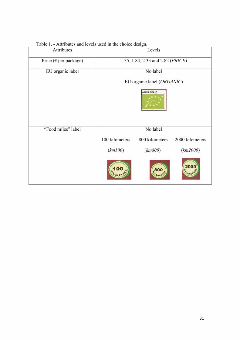
The second step is to choose the attributes and levels to be used. One of the
attributes is obviously the price to allow us to calculate the marginal WTPs. Four
price levels were chosen reflecting price levels found in the Spanish supermarkets
(1.35, Euros, 1.84 Euros, 2.33 Euros, and 2.82 Euros) for a packet of 100 grams of
untoasted almonds. One of the aims of the research project is to examine consumers’
preferences for food products carrying two sustainability related labels: organic and/or
“food miles” labels. Therefore, our second attribute is organic certification with two
levels: either the product has no organic label (conventional product) or the product
has the new EU organic label. The third attribute is “food miles” with four levels. The
first level corresponds with the current situation; in other words, the package of
almonds has no label indicating the number of kilometres that the product has
travelled from the production place. The second level corresponds with a package of
almonds that has been produced within 100 kilometers from Zaragoza city; which in
our case means that it has been produced in the Zaragoza province. The third level
denotes that the almonds have been produced 800 kilometers away (i.e., suggests that
the almonds were produced in some other Spanish region or outside of Spain). The
fourth level denotes that the almonds were produced about 2000 kilometres away
from Zaragoza (i.e., produced outside of Spain). Note that the second level of this
attribute (i.e., 100 kilometers) corresponds also with the definition of locally grown
product4.

13
To avoid deception to participants, almonds were either organic or conventional
and purchased from places matching the distance of transportation indicated in the
“food miles” label. Table 1 shows the attributes and the levels used.
(Insert table 1)
Since it is not realistic to force participants to choose one of the designed
options (Louviere and Street, 2000), each choice set included a no-buy option in
addition to the two almond product options. The choice set design follows Street and
Burgess (2007). In order to not have a high number of choice sets, we used an
orthogonal main effect plan (OMEP) in developing the profiles in the first option
(Street et al., 2005). We then added one of the generators suggested by Street and
Burgess (2007) to obtain the profiles in the second option5. The orthogonal main
effect plan was calculated using the SPSS orthoplan, which generated 16 profiles. We
used these 16 profiles to obtain the products for the second option using one of the
generators derived from the suggested difference vector (1 1 1) by Street and Burgess
(2007) for 3 attributes with 4, 2 and 4 levels, respectively, and the two options. This
design is 95.2% efficient compared to the optimal. Each respondent was asked to
make choices in the 16 choice sets which constituted the main task (task I) of the
experiment.
Theoretical framework
The utility function that would allow us to calculate the marginal WTP of
interest for testing our hypotheses is based on the Lancastrian consumer theory of
utility maximization (Lancaster, 1966), with consumers’ preferences for the attributes
14
modelled within a random utility framework (McFadden, 1974). Lancaster (1966)
proposed that the total utility associated with the provision of a good can be
decomposed into separate utilities for their component attributes. However, this utility
is known to the individual but not to the researcher. The researcher observes some
attributes of the alternatives but some components of the individual utility are
unobservable and are treated as stochastic (Random Utility Theory). Thus, the utility
is taken as a random variable where the utility from the nth individual is based on the
choice among j alternatives within choice set J in each of t choice occasions. In our
empirical specification, the components of the utility function include the different
attributes such as the food labels in the choice experiment, as well as an alternative-
specific constant (ASC) representing the no-buy option. The utility function is
specified as follows:
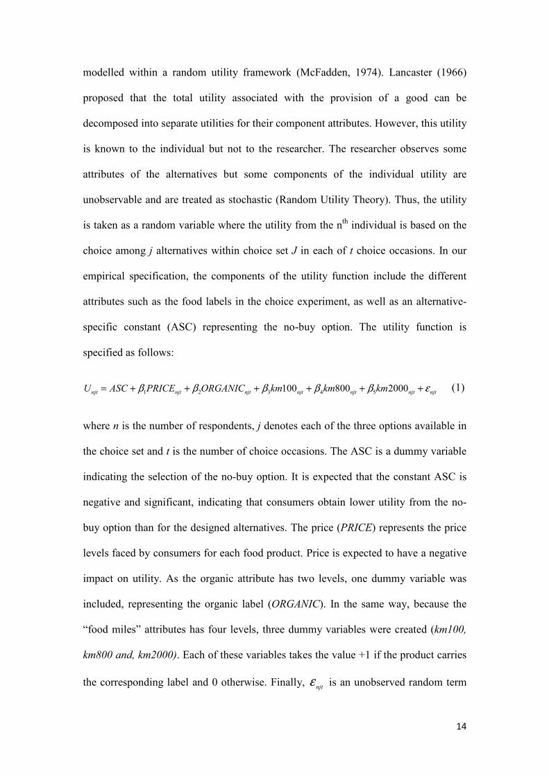
njtnjtnjtnjtnjtnjtnjt kmkmkmORGANICPRICEASCU εβββββ ++++++= 2000800100 54321 (1)
where n is the number of respondents, j denotes each of the three options available in
the choice set and t is the number of choice occasions. The ASC is a dummy variable
indicating the selection of the no-buy option. It is expected that the constant ASC is
negative and significant, indicating that consumers obtain lower utility from the no-
buy option than for the designed alternatives. The price (PRICE) represents the price
levels faced by consumers for each food product. Price is expected to have a negative
impact on utility. As the organic attribute has two levels, one dummy variable was
included, representing the organic label (ORGANIC). In the same way, because the
“food miles” attributes has four levels, three dummy variables were created (km100,
km800 and, km2000). Each of these variables takes the value +1 if the product carries
the corresponding label and 0 otherwise. Finally,
njtε is an unobserved random term

15
that is distributed following an extreme value type I (Gumbel) distribution, i.i.d. over
alternatives and is independent of β and the attributes that is known by the individual
but unobserved and random from the researcher’s perspective. Consumers are
assumed to choose the alternative which provides the highest utility level from those
available.
In our paper we estimated three models: Multinomial Logit Model (MNL),
Random Parameter Logit Model (RPL) (Train, 2003), and Random Parameter Logit
Model with correlated errors (the correlation structure of njt
ε is assumed to follow a
multivariate normal distribution with vector mean µ and variance-covariance matrix
Ω) (Scarpa and Del Giudice, 2004). A number of CE studies have utilized these
models to analyze the responses (Lusk, Roosen, and Fox, 2003; Lusk and Schoroeder,
2004, Tonsor and Shupp, 2011).
Swait and Louviere (1993) stated that although the scale parameter is
unidentifiable within any particular data set, a relative scale parameter across data sets
can be estimated. Because we are using different samples (treatments), it is important
to calculate the relative scale parameter using a MNL model to investigate if
differences in parameter estimates across samples are indeed due to the underlying
preferences or due to difference in variance. In this application, we used an artificial
nested logit model to calculate the relative scale parameter across treatments
(Adamowicz et al., 1998; Hensher and Bradley, 1993; Hensher, Louviere and Swait,
2000; Lusk and Schroeder, 2004). Preference equality was tested by controlling for
difference in scale and by estimating a multinomial logit model that imposes the null
hypothesis of parameter equality across treatments.

16
In accordance with Lusk and Schroeder (2004) we did not control for difference in
scale across treatments in the RPL and RPL with correlated error models. However,
we tested if estimates from the RPL and the RPL with correlated errors models are
equivalent across the five treatments using a test of the joint hypothesis of equality for
both the taste and the scale parameters. If this hypothesis is rejected, comparison of
the estimated WTP across treatments will be appropriate because the scale parameter
is constant within each sample and it will be cancelled out in the calculation of the
marginal WTPs. We tested our hypotheses with regards to differences in marginal
WTPs using the combinatorial test suggested by Poe et al. (1994). This is a non-
parametric test that involves comparing differences in marginal WTP for all possible
combinations of the estimates obtained through the Krinsky-Robb (1986) method. The
combinatorial test has also been similarly applied by Lusk and Schroeder (2004),
Carlsson et al. (2005), Carlsson et al. (2007) and Tonsor and Shupp (2011).
Results
A total of 265 subjects participated in the hypothetical and non-hypothetical
treatments. Table 2 reports the socio-demographic characteristics of the participants in
the five treatments. We used the chi-square test to determine if there are significant
differences in socio-demographic profiles across the five treatments.
The results of the tests also suggest that the null hypothesis of equality between the
socio-demographic characteristics across treatment samples cannot be rejected at the
5% significance level for gender (p-value = 0.969), age (p-value=1.000), education
(p-value = 0.999) and income (p-value = 0.196). This result suggests that our

17
randomization was relatively successful in equalizing the characteristics of
participants across the treatments.
(insert table 2)
Since we first wish to test if the parameters, including the scale parameter (i.e.
error variances), are the same across the treatments, we estimated equation (1) using
a MNL model for each treatment and for two pooled samples. The first pooled
sample is the one with pooled information from the four hypothetical treatments (T1,
CT, NP and HP), while the second one consists of data from the five treatments (T1,
CT, NP, HP and T5). The joint MNL models restrict the estimated parameters to be
equal across treatments and allow for the estimation of the relative scale parameter
(Swait and Louviere, 1993).
Estimations were conducted using NLOGIT 4. First, we estimated five MNL
models, one for each treatment, to get the log likelihood values. We then tested the
null hypothesis of preference equality assuming that parameters are the same in the
two pooled data sets discussed above, with the exception of the scale factor. The test
for equality of preferences is -2 (LLj-Σ LLi) which is distributed χ2 with k (M-1)
degrees of freedom, where LLj is the log likelihood value for the pooled model after
controlling for scale, LLi are the log likelihood values of the different MNL models
from each treatment, K is the number of restrictions and M is the number of
treatments (Swait and Louviere, 1993).
Table 3 shows the results of the MNL estimates. Results indicate that the scales of
hypothetical and non-hypothetical data are statistically equivalent (i.e the relative
scale parameter is not statistically different from 1). Results also suggest that the
hypothesis of equality between the hypothetical and non-hypothetical treatments is

18
rejected (χ2=63.5; p<0.01). Moreover, the hypothesis of equality across hypothetical
choice experiments is also rejected (χ2=66.6; p<0.01). The rejection of these
hypotheses indicates that each treatment (T1, CT, NP, HP and T5) indeed corresponds
to a different cognitive process. Hence, each of the treatments should be considered
separate in further analyses.
(Insert table 3)
To relax the homogeneity assumption of consumers’ preferences, we also
estimated equation (1) using a RPL (Table 4) and a RPL with correlated errors (Table
5) where price is assumed to be fixed and the coefficients for the four dummy
variables are considered random following a normal distribution. For the estimation of
these models, we used 100 Halton draws rather than pseudo-random draws since the
former provides a more accurate simulation for the RPL model (Train, 1999; Train,
2003).
For each random estimation method (RPL and RPL with correlated errors), we
also report the same models presented for the MNL in table 3 and these results are
shown in Table 4 and Table 5. The first joint model pooled data for the five treatments
(T1, CT, NP, HP, T5) while the second joint model pooled data for the four
hypothetical treatments (T1, CT, NP and HP). As mentioned before, following Lusk
and Schroeder (2004), a relative scale parameter was not estimated to determine
whether there were significant differences in variance across the hypothetical and
non-hypothetical treatments. Nonetheless, a likelihood ratio test was calculated to test
the joint hypothesis of equivalence of hypothetical and non-hypothetical taste and
scale parameters in both the RPL and the RPL with correlated errors. The tests of
equality for the RPL and the RPL with correlated errors presented in Table 4 and
19
Table 5 indicate that the joint null hypotheses of equivalence of hypothetical and non-
hypothetical parameters are rejected ensuring that the comparisons of the estimated
WTPs across treatments are appropriate.
Table 4 and Table 5 show that all estimated parameters are statistically significant
and the estimated mean values are consistent across models. Moreover, the standard
deviation parameter estimates are statistically significant in all models implying that
heterogeneity around the mean of the random parameters indeed exists (Hensher et
al., 2005).
( Insert table 4)
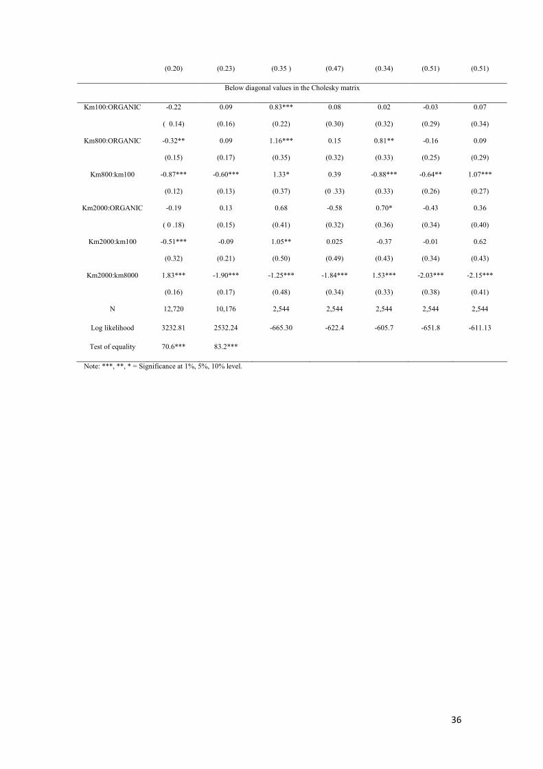
Estimates exhibited in Table 5 show that errors are indeed correlated because most
of the estimated values of the Cholesky matrix are statistically different from zero.
Moreover, if we look at the log likelihood values, we see that the best values are
found in the RPL model with correlated errors across the different model
specifications. Hence, the best fit for our data seems to be the RPL model with
correlated errors (Table 5) and hence, we used this model to calculate the WTPs to
test our research hypotheses.
( Insert table 5)
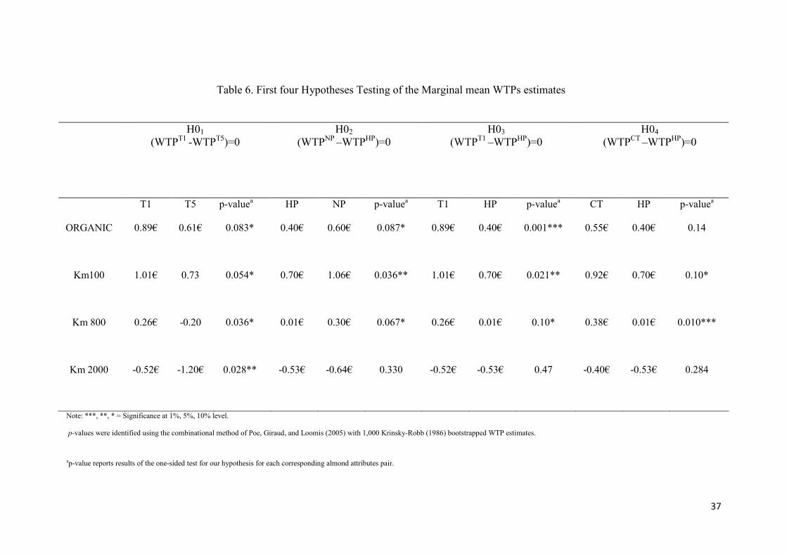
Table 6 reports the marginal WTPs across the five treatments and the
corresponding hypothesis tests. To test our six hypotheses, we used either a one-sided
or two-sided test depending on the alternative hypothesis. Our first hypothesis (H01=
(WTPT1 -WTP
T5)=0; H11= (WTP
T1-WTP
T5 )>0) is rejected in the four analysed labels
(i.e., ORGANIC, km100, km800 and km2000) confirming that WTPs in hypothetical
settings are greater than WTPs in non-hypothetical setting and that hypothetical bias
20
in our baseline hypothetical CE exists. Marginal WTPs in table 6 indicate that the
participants overstated their WTPs across the labels by an average factor of about
1.40. This result is similar to Murphy et al. (2005) and Lusk and Schroeder (2004)
who found a factor of around 1.20.
Our second hypothesis (H02= (WTPNP – WTP
HP)=0; H12= (WTP
NP-WTP
HP
)>0) is rejected in three of the four analysed labels6 confirming that priming effects do
not arise purely due to the nature of the scrambling task but rather due to the
activation of honesty concepts. Moreover, hypothesis 3 (H03= (WTPT1 – WTP
HP)=0;
H13= (WTPT1-WTP
HP )>0) is also rejected in these three labels indicating that
marginal WTPs from the CE using the honesty priming task is lower than those from
our baseline treatment (hypothetical CE without cognitive task). This result implies
that the honesty priming task can reduce the hypothetical bias in hypothetical choice
experiments. In the same way, hypothesis four (H04= (WTPCT – WTP
HP)=0; H14=
(WTPCT-WTP
HP )>0)
is also rejected in two of the four labels
7 suggesting that the
marginal WTPs in the honesty priming treatment are lower than the WTPs in the
cheap talk treatment. While not definitive, this result could suggest that an honesty
priming task can potentially reduce the hypothetical bias more than a cheap talk
script.
(insert table 6)
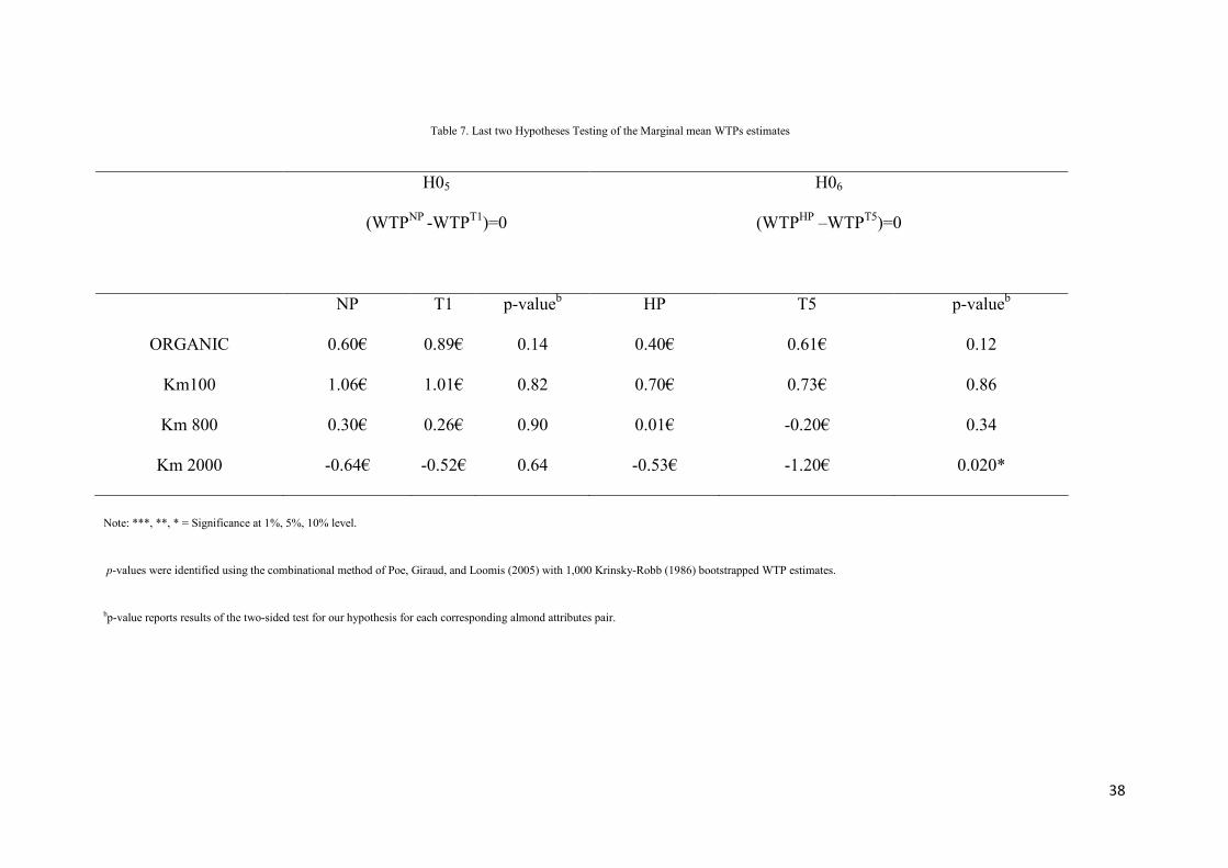
In contrast, we failed to reject the fifth hypothesis H05 (H05= (WTPNP –
WTPT1 )=0;
H15= (WTP
NP-WTP
T1 )#0), which suggests that WTP estimates in neutral
priming treatment (NP) are not statistically different from WTPs in the first treatment
(T1). This result confirms that the neutral priming (NP) treatment did not induce
either a task or priming effect. It also suggests that the scrambled sentence task in
21
itself did not influence the subsequent choice tasks of participants. Finally, we also
failed to reject hypothesis 6 (H06= (WTPHP - WTP
T5 )= 0; H16= (WTP
HP-WTP
T5 )#0)
in three of the four analysed labels8. This result could imply that the honesty priming
task in hypothetical settings could work similarly to the use of an incentive aligned
mechanism in choice experiments. In other words, we could consider a CE with an
honesty priming task as an alternative to the use of a non-hypothetical CE, especially
in cases where it is difficult or challenging to produce the different product profiles or
options needed in the study.
(insert table 7)
As discussed previously, following Ding et al. (2005), we added a hold-out task
(task II) in all the treatments to assess the percentage of correct predictions in each
treatment. We used the estimated parameters in the main task to predict the
respondent’s choices in the hold out task. We then assessed the out of sample
predictions of the estimates by calculating the hit rates. Hit rates are calculated by
comparing the choice predicted for an individual respondent by the model (estimated
parameters), using the maximum utility rule, to the actual choice made by the
respondent. When the model correctly predicts the respondent’s choice, it is counted
as a hit. The hit rate is then calculated by dividing the total number of hits by the total
sample size. The number and percentage of correct predictions across treatments are
displayed in Table 8. We conducted a one tailed z-test of two independent sample
proportions to test whether the five treatments have statistically different predictive
powers. Results suggest that the percentage of correct predictions in the T1
hypothetical treatment is significantly lower than those in the honesty priming (HP)
and non-hypothetical (T5) treatments. Moreover, the percentage of correct predictions
in the honesty priming hypothetical treatment and the non-hypothetical treatment are

22
statistically not different. Percentage of correct predictions in T1, CT, and NP
treatments are below 40% while those in HP and T5 treatments are at least 40%,
which are higher than the hit rates obtained by Ding et al. (2005) for their hypothetical
treatments.
(Insert table 8)
Conclusions
Undoubtedly, the choice experiment (CE) approach is the most widely used
stated preference method in valuing products or attributes in the applied economics
and marketing literature. However, a major issue that has challenged researchers who
use this method is the hypothetical bias issue. Due to the overwhelming evidence
pointing to the existence of hypothetical bias in stated valuation research, non-
hypothetical experimental valuation methods have surfaced in the literature including
non-hypothetical choice experiment (see discussion in Gracia, Loureiro and Nayga
2011). The problem however with using non-hypothetical choice experiment is that
one actually needs to have all the product profiles in the choice sets produced and be
ready to be exchanged for money to make the mechanism incentive aligned. While
making the CE non-hypothetical is noteworthy, it is always not feasible to adopt this
method given the challenges of producing all the product profiles being tested. In
addition to being a relatively new method, this is probably the reason why the
percentage of CE studies conducted non-hypothetically is significantly smaller than
the percentage of CE studies done hypothetically. The hypothetical CE method is also
popularly used in valuation studies dealing with public goods.
Due to the challenge of using the non-hypothetical version of CE, a number of
studies have tested the effectiveness of ex-ante calibration methods such as the cheap
23
talk script in reducing hypothetical bias in CE studies, with mixed results. In this
study, we test an instrument from the social psychology field that has not been tried
before in CE studies: the honesty priming task. In particular, we wished to test
whether exposure to honesty concepts could unconsciously activate honesty among
subjects and let them respond more truthfully and in turn mitigate potential
hypothetical bias in hypothetical choice experiments. Moreover, to investigate if
honesty priming might be an alternative to the use of an incentive aligned mechanism
used in non-hypothetical CE, we also tested if the marginal WTPs from the honesty
priming hypothetical choice experiment are comparable to the marginal WTPs from
the non-hypothetical choice experiment.
Our results generally suggest that the honesty priming task can indeed reduce
the hypothetical bias in hypothetical choice experiments. Specifically, we found that
marginal WTPs in the honesty priming treatment are significantly lower on average
than those in our other hypothetical treatments (i.e., hypothetical without any
cognitive task, hypothetical with cheap talk, and hypothetical with neutral task) but
not statistically different from those in the non-hypothetical treatment. These results
could imply that the change in behavior in the honesty priming treatment is due only
to the honesty priming task and not due to the nature of the scrambling sentence test.
Hence, we suspect that our subjects in the honesty priming treatment have made their
choices in the CE tasks without the influence of experimenter demand effects (i.e.,
they did not relate the aim of the experiment to their subsequent CE task behavior).
We also note that values in the neutral priming treatment were not significantly
different from those in our baseline hypothetical treatment.
Based on the results of our hold out task, we found that one could get higher
correct predictions of participants’ choices in the hypothetical with honesty priming
24
and the non-hypothetical treatments than in the other three hypothetical treatments.
There are generally no significant differences in the percentage of correct predictions
in the hypothetical with honesty priming treatment and the non-hypothetical
treatment.
Overall, our finding seems to suggest that, among all the possible reasons,
untruthful choice revelation is one of the major reasons for the occurrence of
hypothetical bias in hypothetical CE studies, given the effectiveness of the honesty
priming task. Admittedly, this does not necessarily mean that the honesty priming
task in itself could not trigger some other psychological effect that could address the
other reasons for the existence of hypothetical bias (e.g., some subjects may not
exactly know their WTP values), but the results generally point to untruthful
revelation as a major source of the bias.
Our findings hold some promise for the use of honesty priming in mitigating
hypothetical bias in choice experiments. This is an important finding considering the
fact that it is not always possible to conduct a choice experiment non-hypothetically
as discussed above. Our finding implies that if it is not feasible to conduct a choice
experiment non-hypothetically, then one could potentially consider the use of honesty
priming to help mitigate potential hypothetical bias in hypothetical choice experiment
studies. However, as is customary in scientific research, our study represents only
one study and therefore must be replicated in other settings or contexts to test the
robustness of our finding.
25
References
Adamowicz, W. Boxall, R. Williams, M., and Louviere, J. (1998). Stated Preference
Approaches for Measuring Passive Use Value: Choice Experiment and Contingent
Valuation. American Journal of Agricultural Economics, 80 (1): 64-75
Bargh, J. A., Gollwitzer, P. M., Lee-Chai, A. Y., Barndollar, K., and Troetschel, R.
(2001). The automated will: Nonconscious activation and pursuit of behavioral
goals. Journal of Personality and Social Psychology, 81: 1014-1027.
Brummett, R. G., R. M. Nayga, and X. Wu (2007). On the Use of Cheap Talk in New
Product Valuation. Economics Bulletin 2:1–9.
Cameron, T., Poe, G., Ethier, R., and Schulze, W. (2002). Alternative Non-Market
Value-Elicitation Methods: Are the Underlying Preferences the Same? Journal of
Environmental Economics and Management, 44: 391-425.
Carlsson, F., P. Martinsson (2001), Do hypothetical and actual marginal willingness
to pay differ in choice experiments? Application to the valuation of the
environment. J. Environ. Econ.Manage. 41(2): 179-192.
Carlsson, F., Frykblom, P. and Lagerkvist, C.-J. (2005). Using cheap talk as a test of
validity in choice experiments. Economics Letters 89: 147–152.
Carlsson, F., Frykblom, P. and Lagerkvist, C.-J. (2007). Consumer willingness to pay
for farm animal welfare: mobile abattoirs versus transportation to slaughter.
European Review of Agricultural Economics 34(3): 321–344.

26
Chang JB, Lusk J, Norwood FB (2009) How closely do hypothetical surveys and
laboratory experiments predict field behaviour? American Journal of Agricultural
Economics 91(2):518-534
Chartrand, T.L., Huber, J., Shiv, B. and Tanner, R.J. (2008). Nonconscious goals and
consumer choice. Journal of Consumer Research 35, 189-201.
Cummings, R. G. and L. O. Taylor (1999). Unbiased Value Estimates for
Environmental Goods: A Cheap Talk Design for the Contingent Valuation
Method. The American Economic Review, 89, 649–665.
Ding, M., Grewal, R, and Liechty, J. (2005). Incentive-Aligned Conjoint Analysis.
Journal of Marketing Research, Vol. 42: 67-82
Gracia, A., Loureiro, M.L., and Nayga, R. Jr. (2011). Are Valuation from
Nonhypothetical Choice Experiments different from those of Experimental
Auctions? American Journal of Agricultural Economics, 93(5): 1358-133
Groves, A. 2005. The local and regional food opportunity. IGD
http://www.defra.gov.uk/foodfarm/food/industry/regional/pdf/localregfoodopps.p
df.
Hensher D.A., Rose J.M., Greene W.H. (2005) Applied choice analysis. A primer.
Cambridge University Press. New York.
Hensher, D. A. (2010). Hypothetical bias, choice experiments and willingness to pay.
Transportation Research Part B 44 (2010) 735–752
Hensher, D.A. amd Bradley, M. (1993). Using Stated Response Choice Data to Enrich
Revealed Preferences Discrete Choice Models. Marketing Letters, 4: 139-51

27
Kay, A. C. and Ross, L. (2003). The perceptual push: The interplay of implicit cues
and explicit situational construals on behavioral intentions in the Prisoners’
Dilemma. Journal of Experimental Social Psychology, 39: 634–643.
Johansson-Stenman O, Svedsäter H (2008). Measuring hypothetical bias in choice
experiments: The importance of cognitive consistency. The Berkeley Electronic
Journal of Economic Analysis and Policy, 8(1): article 41. Available at:
http://www.bepress.com/bejeap/vol8/iss1/art41
Krinsky, I. and A.L. Robb(1986). “On Approximating the Statistical Properties of
Elasticities.” Review of Economics and Statististics 64:715–19.
Lancaster, K. A (1966) New Approach to Consumer Theory. Journal of Political
Economy, 74: 132-157.
List, J.A., and Gallet, G. A. (2001). What Experimental Protocol Influence Disparities
Between Actual and Hypothetical State Value?. Environmental and Resource
Economics, 20: 241-254.
List, J. A. (2001). Do Explicit Warnings Eliminate the Hypothetical Bias in Elicitation
Procedures? Evidence from Field Auctions for Sportscards. American Economic
Review, 91: 1498–1507.
Loomis J, Bell P, Cooney H, Asmus C (2009). A comparison of actual and
hypothetical willingness to pay of parents and non-parents for protecting infant
health: The case of nitrates in drinking water. Journal of Agricultural and Applied
Economics, 41(3):697-712
Hensher, D.A., Louviere, J.J., and Swait, J. (2000). State Choice Methods Analysis
and Application. Cambridge: Cambridge University Press
28
La Trobe, H., 2001. Farmers’ markets: consuming local rural produce. International
Journal of Consumer Studies, 25(3), 181-192.
Louviere, J.J. and D. Street. (2000). Stated-preference Methods. In David A Hensher
& Kenneth J Button (eds), Handbook of Transport Modelling, Pergamon Press,
Amsterdam, Netherlands.
Lusk, J.L.(2003) ―Effect of Cheap Talk on Consumer Willingness-to-Pay for Golden
Rice.‖ American Journal of Agricultural Economics. 85:840-56.
Lusk, J.L., J. Roosen, and J.A. Fox. ―Demand for Beef from Cattle Administered
Growth Hormones or Fed Genetically Modified Corn: A Comparison of Consumers
in France, Germany, the United Kingdom, and the United States‖ American Journal
of Agricultural Economics. 85(2003):16-29
Lusk, J.L, and Schroeder, T.C. (2004). Are Choice Experiment Incentive Compatible:
A Test of Quality Differentiate Beef Steak. American Journal of Agricultural
Economics, 86: 567-82.
Maxwell, S., Nye, P. and Maxwell, N. (1999). Less Pain, Same Gain: The Effects of
Priming Fairness in Price Negotiations. Psychology & Marketing, 16: 545–62.
McFadden, D., (1974). ''Conditional Logit Analysis of Qualitative Choice Behavior''.
In P. Zarembka (Ed.), Frontiers in econometrics (pp. 105–142). New York:
Academic Press.
Murphy, J.J, Geoffrey, J.A.,Stevens, T.H., and Weatherhead, D. (2005). Meta-
Analysis of Hypothetical Bias in Stated Preference Valuation, Environmental and
Resource Economics, 30: 313–325.
29
Poe, G. L., Giraud, K. L. and Loomis, J. B. (2005). Computational methods for
measuring the difference of empirical distributions. American Journal of
Agricultural Economics, 87(2): 353–365.
Scarpa R, Del Giudice T (2004). Market segmentation via mixed logit: extra-virgin
olive oil in urban Italy. Journal of Agricultural and Food Industrial Organization
2: article 7.
Silva, A.,. Nayga, R. Jr.,. Campbell, B. L, and L. Park L. J. (2011). Revisiting Cheap
Talk with New Evidence from a Field Experiment. Journal of Agricultural and
Resource Economics, 36(2):280–291
Street D, Burgess L, Louviere J. (2005). Quick and easy sets: Constructing optimal
and nearly optimal stated choice experiment. International Journal of Research in
Marketing, 22:459-470.
Street, D. and Burgess, L. 2007. The Construction of Optimal Stated Choice
Experiments (New Jersey: John Wiley & Sons Inc.
Swait, J, and Louviere, J. (1993). The role of the Scale Parameter in the Estimation
and Use of Multinomial Logit Models. Journal of Marketing Research, 30:305-14
Tonson, G.T. and Shypp, R.S. (2011). Cheap talk scripts online choice Experiment:
Looking beyond the Mean. American Journal of Agricultural Economics, 93(4):
1015-1031.
Train K (2003) Discrete choice methods with simulation. Cambridge University
Press, Cambridge, 334 pp.
Train, K (1999). Halton sequences for mixed logit. ELSA Berkley Working Paper
08/99, Berkley (CA).

30
1 Marginal mean WTP values for attributes are calculated by taking the ratio of the
mean parameter estimated for the non-monetary attributes to the mean price parameter
multiplied by minus one.
2 We are grateful to Dirk Smeesters for helpful comment on this.
3 We are grateful to Min Ding for helpful comment on this.
4 Groves (2005) and La Trobe (2001) consider local food products as those produced
and sold within a 30-150 mile radius of a consumer’s residence.
5 This design allows us only to estimate the main effects.
6 Except for the km2000 label whose WTPs are not statistically different but negative,
the marginal WTP estimates for organic, km100 and km800 labels are statistically
lower in the honesty priming (HP) treatment than in the neutral priming (NP)
treatment.
7 Marginal WTPs estimates for km100 and km800 labels in the honesty priming
treatment are lower than the WTPs in the cheap talk treatment while the marginal
WTPs for organic and km2000 are statistically equal in both treatments.
8 Marginal WTPs estimates for organic, km100 and km800 labels are statistically
equal in the honesty priming (HP) treatment and in the non-hypothetical treatment
(T5), while the marginal WTP estimates for km2000 in the non-hypothetical treatment
is lower than in the honesty priming treatment.
31
Table 1. - Attributes and levels used in the choice design.
Attributes Levels
Price (€ per package) 1.35, 1.84, 2.33 and 2.82 (PRICE)
EU organic label No label
EU organic label (ORGANIC)
“Food miles” label No label
100 kilometers 800 kilometers 2000 kilometers
(km100) (km800) (km2000)

32
Table 2. Sample characteristics (%).
Variable definition T1 CT NP HP T5
Gender
Male
Female
49.0
51.0
45.2
54.7
49.0
51.0
45.3
54.7
51.0
49.0
Age
Between 18-35 years
Between 35-54 years
Between 55-64 years
More than 64 years
24.5
35.8
16.9
22.6
26.4
37.7
15.0
20.7
25.0
38.5
15.4
21.1
30.2
32.0
15.0
21.1
28.3
32.0
18.8
20.7
Education of respondent
Elementary School
High School
University
26.4
39.6
34.0
22.6
45.3
32.0
22.6
41.5
35.8
24.5
37.7
37.7
24.5
39.6
35.8
Average household monthly
net income
Lower than 900 €
Between 900 and 1,500 €
Between 1,501 and 2,500 €
Between 2,501 and 3,500 €
More than 3,500 €
9.4
22.6
28.3
20.7
18.9
20.7
18.8
26.4
20.7
13.2
9.4
5.6
33.9
32.0
18.8
9.4
15.0
30.2
30.2
15.0
5.7
13.2
47.2
18.9
15.0

33
Table 3. Multinomial Logit model estimates: comparison of hypothetical and non-hypothetical treatments.
Hypothetical and non-hypothetical Hypothetical
T1+CT+NP+HP+
T5
T1+CT+HP+NP T5 T1+CT+HP+NP
T1
CT
HP
NP
Parameters
(t-ratios)
Parameters
(t-ratios)
Parameters
(t-ratios)
Parameters
(t-ratios)
Parameters
(t-ratios)
Parameters
(t-ratios)
Parameters
(t-ratios)
Parameters
(t-ratios)
PRICE 0.86***
(0.03)
-0.58***
(0.03)
-0.61***
(0.05)
-0.53***
(0.02)
-0.41**
(0.05)
-0.81***
(0.06)
-0.67***
(0.06)
-0.45***
(0.05)
ORGANIC 1.34***
(0.05 )
1.26***
(0.05 )
0.96***
(0.10 )
0.98***
(0.04 )
1.17***
(0.09)
1.22***
(0.10)
0.94***
(0.10)
0.99***
(0.09)
Km100 0.58***
(0.05 )
1.74***
(0.07 )
1.21***
(0.13 )
1.59***
(0.06 )
1.59***
(0.14)
1.93***
(0.15)
1.77***
(0.14)
1.76***
(0.14)
Km 800 -0.14***
(0.05 )
0.83***
(0.07 )
0.25
(0.15)
0.76***
(0.07 )
0.71***
(0.15)
1.06***
(0.16)
0.75***
(0.15)
0.86***
(0.15)
Km 2000 -0.48
(0.02 )
-0.06
(0.07 )
-0.70***
(0.16 )
-0.05
(0.06)
-0.08
(0.14)
0.04
(0.16 )
0.04
(0.15)
-0.45***
(0.05)
Scale parameter 1.21***
(0.06)
1.09**
(0.03)
N 12,720 10,176 2,544 10,176 2,544 2,544 2,544 2,544
Log likelihood -3,880.6 -3,063.0 -785.2 -3,063.0 -756.0 -735.5 -775.4 -763.1
Test of equality 63.6*** 66.6***
Note: ***, **, * = Significance at 1%, 5%, 10% level.

34
Table 4. Random Parameter model estimates: comparison of hypothetical and non-
hypothetical treatments.
Hypothetical and non-hypothetical Hypothetical
T1+CT+NP+HP+T5 T1+CT+HP+NP T5 T1 CT HP NP
Parameters
(t-ratios)
Parameters
(t-ratios)
Parameters
(t-ratios)
Parameters
(t-ratios)
Parameters
(t-ratios)
Parameters
(t-ratios)
Parameters
(t-ratios)
ASC -3.17***
(0.13)
-3.38***
(0.15)
-2.46***
(0.29)
-3.10***
(0.31)
-3.11***
(0.32)
-3.88***
(0.32)
-3.78***
(0.33)
PRICE -1.87***
(0.06)
-1.96***
(0.07)
-1.63***
(0.13)
-1.65***
(0.14)
-2.17***
(0.16)
-2.23***
(0.15 )
-1.96***
(0.14)
ORGANIC 1.10***
(0.09)
1.14***
(0.11)
0.92***
(0.19)
1.21***
(0.22)
1.08***
(0.24)
0.93***
(0.17)
1.12***
(0.23)
Km100 1.58***
(0.09)
1.75***
(0.11)
0.99***
(0.19)
1.76***
(0.24)
1.97***
(0.23)
1.55***
(0.21)
1.94***
(0.26)
Km 800 0.25**
(0.10)
0.37***
(0.11)
-0.41
(0.29)
0.21
(0.23)
0.74***
(0.23)
-0.004
(0.21)
0.37*
(0.23)
Km 2000 -1.10***
(0.13)
-1.01***
(0.15)
-1.82***
(0.36)
-0.93***
(0.30)
-0.82***
(0.27)
-1.12***
(0.32)
-1.20***
(0.33)
Standard deviations of parameter distributions
ORGANIC 1.34***
(0.08)
1.46***
(0.11)
1.04***
(0.16)
1.84***
(0.23)
1.77***
(0.25)
0.88***
(0.15)
1.52***
(0.19)
Km100 1.01***
(0.09)
1.06***
(0.12)
0.82***
(0.18)
1.17***
(0.27)
1.03***
(0.24)
0.93***
(0.22)
1.36***
(0.30)
Km 800 0.91***
(0.12)
0.87***
(0.13)
1.60***
(0.34)
0.94***
(0.24)
0.78***
(0.23)
0.62**
(0.31)
0.86***
(0.23)
Km 2000 1.62***
(0.14)
1.62***
(0.15)
1.40***
(0.31)
1.64***
(0.26)
1.07***
(0.22)
1.85***
(0.36)
1.84***
(0.35)
N 12,720 10,176 2,544 2,544 2,544 2,544 2,544
Log
likelihood
-3,314..0 -2,591.6 -696.1 -632.3 -626.5 -662.6 -626.6
Test of
equality
52.9*** 78.0***
Note: ***, **, * = Significance at 1%, 5%, 10% level.

35
Table 5. Random Parameter model estimates with correlated errors: comparison of
hypothetical and non-hypothetical treatments.
Hypothetical and non-
hypothetical
Hypothetical
T1+CT+NP+
HP+T5
T1+CT+
HP+NP
T5 T1
CT
HP
NP
Parameters
(t-ratios)
Parameters
(t-ratios)
Parameters
(t-ratios)
Parameters
(t-ratios)
Parameters
(t-ratios)
Parameters
(t-ratios)
Parameters
(t-ratios)
ASC -3.16***
(0.13)
-3.42***
(0.15)
-2.42***
(0.28)
-3.07***
(0.31)
-3.25***
(0.33)
-3.90***
(0.32)
-3.76***
(0.33)
PRICE -1.84***
(0.06)
-1.96***
(0.07)
-1.55***
(0.13)
-1.60***
(0.14)
-2.20***
(0.16)
-2.24***
(0.15)
-1.96***
(0.15)
ORGANIC 0.98***
(0.09)
1.11***
(0.10)
0.95***
(0.16)
1.42***
(0.24)
1.21***
(0.23)
0.90***
(0.19)
1.17***
(0.24)
Km100 1.57***
( 0.10)
1.81***
(0.13)
1.14***
(0.21)
1.77***
(0.26)
2.03***
(0.25)
1.59***
(0.23)
0.09***
(0.29)
Km 800 0.23***
(0.11)
0.49***
(0.12)
-0.32
(0.31)
0.42
(0.26)
0.83***
(0.28)
0.03
(0.24)
0.59**
(0.28)
Km 2000 -1.28***
(0.16)
-0.96***
(0.17)
-1.87***
(0.39)
-0.85***
(0.37)
-0.88***
(0.31)
-1.19***
(0.34)
-1.26***
(0.38)
Standard deviations of parameter distributions
ORGANIC 1.33***
( 0.10)
1.43***
(0.11)
0.89***
(0.17)
1.72***
(0.26)
1.53***
(0.23)
1.02***
(0.18)
1.80***
(0.25)
Km100 1.11***
( 0.10)
1.20***
(0.11)
1.07***
(0.21)
1.13***
(0.27)
1.23***
(0.24)
1.14***
(0.25)
1.53***
(0.26)
Km 800 1.31***
( 0.12)
1.15***
(0.12)
1.86***
(0.39)
0.96**
(0.21)
0.99***
(0.25)
1.07***
(0.23)
1.50***
(0.24)
Km 2000 1.93***
(0.16)
1.91***
(0.17)
1.84***
(0.69)
1.95
(0.37)
0.01
(0.32)
2.08***
(0.36)
2.32***
(0.40)
Diagonal values in Cholesky matrix
Ns ORGANIC 1.33***
(0.10)
1.43***
(0.01)
0.89***
(0.15)
1.72***
(0.26)
1.53***
(0.23)
1.02***
(0.18)
1.80***
(0.25)
Ns km100 1.08***
(0.10)
1.19***
(0.11)
0.68***
(0.21)
1.13***
(0.27)
1.23***
(0.25)
1.14***
(0.25)
1.53***
(0.26)
Ns km800 0.92***
0.10
0.97***
(0.11)
0.57 *
( 0.24)
0.88**
(0.21)
1.56***
(0.30)
0.84***
(0.21)
1.04***
(0.24)
Ns km2000 0.28 0.03 0 .48 0.24 1.72*** 0.15 0.46
36
(0.20) (0.23) (0.35 ) (0.47) (0.34) (0.51) (0.51)
Below diagonal values in the Cholesky matrix
Km100:ORGANIC -0.22
( 0.14)
0.09
(0.16)
0.83***
(0.22)
0.08
(0.30)
0.02
(0.32)
-0.03
(0.29)
0.07
(0.34)
Km800:ORGANIC -0.32**
(0.15)
0.09
(0.17)
1.16***
(0.35)
0.15
(0.32)
0.81**
(0.33)
-0.16
(0.25)
0.09
(0.29)
Km800:km100 -0.87***
(0.12)
-0.60***
(0.13)
1.33*
(0.37)
0.39
(0 .33)
-0.88***
(0.33)
-0.64**
(0.26)
1.07***
(0.27)
Km2000:ORGANIC -0.19
( 0 .18)
0.13
(0.15)
0.68
(0.41)
-0.58
(0.32)
0.70*
(0.36)
-0.43
(0.34)
0.36
(0.40)
Km2000:km100 -0.51***
(0.32)
-0.09
(0.21)
1.05**
(0.50)
0.025
(0.49)
-0.37
(0.43)
-0.01
(0.34)
0.62
(0.43)
Km2000:km8000 1.83***
(0.16)
-1.90***
(0.17)
-1.25***
(0.48)
-1.84***
(0.34)
1.53***
(0.33)
-2.03***
(0.38)
-2.15***
(0.41)
N 12,720 10,176 2,544 2,544 2,544 2,544 2,544
Log likelihood 3232.81 2532.24 -665.30 -622.4 -605.7 -651.8 -611.13
Test of equality 70.6*** 83.2***
Note: ***, **, * = Significance at 1%, 5%, 10% level.
37
Table 6. First four Hypotheses Testing of the Marginal mean WTPs estimates
H01 (WTP
T1 -WTP
T5)=0
H02 (WTP
NP –WTP
HP)=0
H03 (WTP
T1 –WTP
HP)=0
H04 (WTP
CT –WTP
HP)=0
T1 T5 p-valuea
HP NP p-valuea T1 HP p-value
a CT HP p-value
a
ORGANIC 0.89€ 0.61€ 0.083*
0.40€ 0.60€ 0.087* 0.89€ 0.40€ 0.001*** 0.55€ 0.40€ 0.14
Km100 1.01€ 0.73 0.054*
0.70€ 1.06€ 0.036** 1.01€ 0.70€ 0.021** 0.92€ 0.70€ 0.10*
Km 800 0.26€ -0.20 0.036*
0.01€ 0.30€ 0.067* 0.26€ 0.01€ 0.10* 0.38€ 0.01€ 0.010***
Km 2000 -0.52€ -1.20€ 0.028**
-0.53€ -0.64€ 0.330 -0.52€ -0.53€ 0.47 -0.40€ -0.53€ 0.284
Note: ***, **, * = Significance at 1%, 5%, 10% level.
p-values were identified using the combinational method of Poe, Giraud, and Loomis (2005) with 1,000 Krinsky-Robb (1986) bootstrapped WTP estimates.
ap-value reports results of the one-sided test for our hypothesis for each corresponding almond attributes pair.
38
Table 7. Last two Hypotheses Testing of the Marginal mean WTPs estimates
H05
(WTPNP
-WTPT1)=0
H06
(WTPHP –WTP
T5)=0
NP T1 p-valueb
HP T5 p-valueb
ORGANIC 0.60€ 0.89€ 0.14 0.40€ 0.61€ 0.12
Km100 1.06€ 1.01€ 0.82 0.70€ 0.73€ 0.86
Km 800 0.30€ 0.26€ 0.90 0.01€ -0.20€ 0.34
Km 2000 -0.64€ -0.52€ 0.64 -0.53€ -1.20€ 0.020*
Note: ***, **, * = Significance at 1%, 5%, 10% level.
p-values were identified using the combinational method of Poe, Giraud, and Loomis (2005) with 1,000 Krinsky-Robb (1986) bootstrapped WTP estimates.
bp-value reports results of the two-sided test for our hypothesis for each corresponding almond attributes pair.

39
Table 8 Comparisons of Number and Percentage of correct prediction across
treatments.
Treatment Number of
correct
prediction
% p-valuea
14 26 0.05** T1
T5 22 42
21 40 0.41 HP
NP 17 32
21 40 0.07* HP
T1 14 26
21 40 0.69 HP
CT 19 36
14 26 0.26 T1
NP 17 32
22 42 0.42 T5
HP 21 40
a p-value reports results of the one-sided test that number of correct prediction in T5 is > of number of correct prediction in
hypothetical setting; and that number of correct prediction in HP is > of number of correct prediction in hypothetical setting.

40
Annex 1
Cheap talk treatment (Cummings and Taylor, 1999).
Studies show that people tend to act differently when they face hypothetical decisions.
In other words, they say one thing and do something different. For example, some
people state a price they would pay for an item, but they will not pay the price for the
item even when they see this product in a grocery store.
There can be several reasons for this different behavior. It might be that it is too difficult
to measure the impact of a purchase in the household budget. Another possibility is that
it might be difficult to visualize themselves getting the product from a grocery store
shelf and paying for it. Do you understand what I am talking about?
We want you to behave in the same way that you would if you really had to pay for the
product and take it home. Please take into account how much you really want the
product, as opposed to other alternatives that you like or any other constraints that might
make you change your behavior, such as taste or your grocery budget. Please try to
really put yourself in a realistic situation
Neutral treatment (NP)
Before participating in the Choice experiment task, for each set of words below, please
develop a grammatically correct sentence and write it down in the space provided. You
do not have to take into account all the words in each sentence
For example:
This is Zaragoza Capital Aragón of the
Zaragoza is the capital of Aragón
1. earth is white round the
2. tomatoes are up red
3. whales live in oceans the
4. this summer table hot is
5. makes baker bread drink
6. like basketball he I
7. milk give cows the
8. thirst of the water removed he sensation the
9. sweet the is cake are
10. works laptop the this
11. up is in cold winter it
12. are not classes summer out there in
13. going I theatre like the to
14. usually he home they I lunch have at
15. to tomorrow cinema I go will the
16. the in morning in drink coke I

41
17. october in I go will for trip a
18. Christmas in holidays are here there
19. is the snow white black
20. girl Spanish the is
21. the country dinner was delicious
22. years make piano he has been playing for
23. as a chef he working is slippers
24. from his friends nice are
Honesty treatment
Before participating in the Choice experiment task, for each set of words below, please
develop a grammatically correct sentence and write it down in the space provided. You
do not have to take into account all the words in each sentence
For example:
This is Zaragoza Capital Aragón of the
Zaragoza is the capital of Aragón
1. person honest this red is
2. earth is white round the
3. must always tell you truth sun the
4. tomatoes are the up red
5. whales live in oceans the
6. she interest genuine learning in has a
7. Summer table hot is in
8. met I person week fair a
9. explanation is honest this an
10. within seem your to be opinions genuine
11. sincerity is your reflected in behavior your from
12. makes baker bread drink
13. man is this fair market
14. the table honesty is human a quality
15. words his are sincere are
16. like basketball he I
17. honestly talk usually I round
18. opinions are your fair from
19. milk give cows the
20. person a over sincere met I
21. thirst the water removed he the
22. says she always lunch truth the
23. true this is a story earth
24 wallet the is of genuine leather this
N.B. Note: Subjects did not see the words in bold but in normal font