Embed Size (px)
Citation preview

Centrifugal Contactors: Separationof an Aqueous and an Organic Stream in
the Rotor Zone (LA-UR-05-7800)
Nely T. Padial-Collins, Duan Z. Zhang, Qisu Zou, and Xia Ma
Computer and Computational Sciences Division Group CCS-2,
Continuum Dynamics, Los Alamos, New Mexico, USA
W. Brian VanderHeyden
Nonproliferation & Security Technology Program Office (N-NST),
Washington, DC, USA
Abstract:Amulti-phase flowcode is used to simulate the separation of an aqueous and an
organic stream in the rotor zone of an annular centrifugal contactor. Different values for
themixture viscosity and for the initial volume fractions of the components are considered.
A simplemodel for mass transfer of a species between phases is used. Geometrical effects
are found to have significant influence on the separation of the two-phase mixture.,
Keywords: Separation, multi-phase flow, mixture viscosity, mass transfer, numerical
simulation
INTRODUCTION
The development of annular centrifugal contactors began at the National
Laboratories more than three decades ago. The first centrifugal contactors
were devised at the Savannah River Laboratory (SRL) and, subsequently
Received 18 October 2005, Accepted 7 February 2006
This work was carried out under the auspices of the National Nuclear Security
Administration of the U.S. Department of Energy at Los Alamos National Laboratory
under Contract No. W-7405-ENG-36.
Address correspondence to Nely T. Padial-Collins, Computer and Computational
Sciences Division Group CCS-2, Continuum Dynamics, MS D413, Los Alamos,
New Mexico, 87544, USA. E-mail: [email protected]
Separation Science and Technology, 41: 1001–1023, 2006
Copyright # Taylor & Francis Group, LLC
ISSN 0149-6395 print/1520-5754 online
DOI: 10.1080/01496390600641611
1001

modified at Argonne National Laboratory (ANL) to the form known as the
annular centrifugal contactor. A reasonably complete description of the
technology has been provided in papers by ANL scientists (1–4). The contactors
consist of a vertical centrifugeproviding for both themixing and for the separating
of liquids in a single unit. They can be easily interconnected to allow multistage
processing. In each contactor, two immiscible liquids are fed into the annulus,
formed by the spinning rotor and the stationary housing wall, through different
inlets close to the top of the device. The liquids mixed in the annular region are
pumped into the rotor bottom. Upon entering the rotor region or separation
zone, the liquids are accelerated to the wall with the heavier fluid going to the
outside. Each liquid leaves the device through an exit port. Transfer of a
species between the two phases depends on the extent of the contacting
surface, on the separation between the two phases, and the time of contact
between the phases.
A large part of the prediction and analysis of the results of centrifugal
contactor experiments has been made, chiefly, through flow sheet simulations,
which treat unit operations like the contactor device as a black box. The con-
struction of the flow sheet simulations utilizes mass and species conservation
equations, chemical and thermodynamic data to fit experimental data to equi-
librium equations (see, for example, references (5–7). The flow sheet simu-
lations give the component concentration of every stage at steady-state as
well as an estimate of the time to reach the steady-state. In addition, some
fluid dynamical simulations have been performed for the two-fluid Taylor-
Couette flow with an inner rotating cylinder and a stationary outer cylinder
similar to the conditions of the mixing zone in a contactor (8, 9). Another
study investigates the two-fluid Taylor-Couette flow in the gap between
concentric, co-rotating cylinders (10).
In this paper, we simulate the separation of an aqueous and an organic
stream in the rotor zone of one single contactor used in the actinide processing
industry. We study the influence of the initial Organic to Aqueous (O/A) ratioinside the separation zone under the inflow of equal amounts of organic and
aqueous materials. We show 2-dimensional (2D) simulations with the cylind-
rical symmetry of the separation zone. We, also, show 3-dimensional (3D)
simulations of the same region. In these simulations, we have used the
CartaBlanca (11) computer simulation program. This is a state-of-the-art
multi-phase flow code environment, which uses advanced software design,
and advanced nonlinear solver methods for the solution of multiphase flow
equations on unstructured grids and complex geometries.
In addition to solvent extraction processes for metal-based solutes, the
annular centrifugal contactor has been employed in other fields, as for
example, the Pharmaceutical Industry (12) and in the Agricultural Food
Products purification (13).
In what follows, we discuss the theoretical aspects of the calculations
including the theoretical tools for the problem set up, the results and
conclusions of our calculations.
N. T. Padial-Collins et al.1002

THEORETICAL SECTION
Governing Equations
In this study, the isothermal flows require only mass and momentum conserva-
tion equations. The mass conservation equation for each phase, denoted by the
index k, is:
@ukrk@t
þ r � ukrk~uk ¼ 0; ð1Þ
where rk is the constant mass density, ~uk is the velocity, and uk is the volume
fraction of the phase k satisfying the continuity condition,P
k uk ¼ 1. The
momentum equation for each phase is given in the inertial frame by:
@ukrk~uk@t
þ r � ðukrk~uk~ukÞ ¼ �ukrpþXl=k
Fkl þ ukrk~gþ ukr � tm ð2Þ
where p is the pressure, Fkl is the momentum exchange force between phase k
and phase l, ~g is the gravity acceleration, and tm is the average viscous stress
for the mixture. We model the stress as tm ¼ 2mmixture Emixture, where mmixture
is the effective viscosity of the mixture, and Emixture is the mixture strain
rate calculated from the gradient of the mixture velocity ~um ¼P
k uk~uk. Theeffective mixture viscosity can incorporate different physical effects and
be a function not only the viscosities of the two phases and of the volume
fraction, but also a function of the state of the flow. Given the lack of
experimental data, we study numerically only the relative importance of the
effective viscosity of the mixture by employing a simple model discussed in
the Calculation Tools part of this section.
In this calculation, we consider only the momentum exchange due to
drag:
Fkl ¼ ukulKklð~ul � ~ukÞ; ð3Þ
where Kkl is the momentum exchange coefficient. We model the momentum
exchange coefficient using the model appropriate to a particulate or droplet
phase dispersed throughout a continuous phase
Kkl ¼3
4r0klCd
j~ul � ~ukj
dklð4Þ
In equation (4), rkl0 is the material density of the continuous phase and Cd
is the drag coefficient. The following relation between a spherical droplet with
diameter dkl and a Newtonian fluid was used
Cd ¼ Cd1 þ24
Rekl
þ6
ð1þffiffiffiffiffiffiffiffiRe
kl
pÞ; ð5Þ
Centrifugal Contactors 1003

with
Rekl¼
j~uk � ~uljdklnkl
ð6Þ
where nkl is the continuous phase kinematics viscosity. The expression in
equation (5) is due to White (14). For this study, we had to estimate an
effective droplet diameter since we did not have any direct observations of
the droplets. We used a value of 0.015 cm based on a calibration which repro-
duces the measured (15) settling time from a simple experiment under the
force of gravity.
A very important aspect of the liquid–liquid extraction is the mass
transfer of a solute component from one of the phases to the other. We can
describe the transfer of one component, in phase l with mass fraction xl to
the phase k through the equations:
@ulrlxl@t
þ r � ðulrlxl~ulÞ ¼ ulukKMTlk ðxl � gxkÞ
@ukrkxk@t
þ r � ðukrkxk~ukÞ ¼ �ulukKMTlk ðxl � gxkÞ
ð7Þ
where the right hand side represents interphase mass transfer via a simple
linear law. Here, KlkMT is the mass transfer coefficient and g is the equilibrium
distribution ratio. For demonstration purposes and for lack of better infor-
mation on the mass transfer rates and equilibria, we use KklMT ¼ 1.0 and
g ¼ 0.1 to calculate the mass transfer of one of the species in the aqueous
phase l to the organic phase k. Once parameters are determined from further
analyses, the method can be repeated with the appropriate values.
Calculations Tools
The Computational Meshes
In this study, we represent the separation zone of the contactor through 2D and
3D unstructured meshes. Figure 1 shows the three-dimensional mesh used in
this calculation while Figure 2 shows both two-dimensional meshes used. The
first one has vertical walls, the second one is inclined in relation to the vertical.
The inclined-wall mesh was used to explore the effect of the geometry in the
efficiency of the centrifugal contactors. Boycott (16) demonstrated, as long
ago as 1920, that particles separated much faster from liquid by sedimentation
if the container is tilted in relation to the direction of settling dictated by
gravity. We have applied the same idea to the centrifugal contactors by
designing the chamber with tilted sides.
The separation zone is 15.0 cm high. The internal radii are 0.3 cm and
0.8 cm above and below the diverter disc respectively. The diverter disc has
N. T. Padial-Collins et al.1004

a 1.25 cm radius. We simplified the weirs at the top of the region considerably
since we were interested only in the separation zone itself.
With the 2D meshes, we use the cylindrical symmetry capability of Carta-
Blanca. In this case, the mixture flows into the region through an opening in the
base. Considering the cylindrical symmetry, this represents an inflow through a
ring. There are two outlets as indicated in the figure. In the upper inner outlet,
we impose a pressure boundary condition. In the lower outer outlet, we impose a
specified velocity boundary condition. Again, due to the cylindrical symmetry,
these outlets represent the outflow through a circular region. The 3D mesh is a
quarter section of the region.The liquids leave either through small holes, in a
3D mesh calculation or through circular outlets when using a 2D mesh and
cylindrical symmetry. The meshes are unstructured.
Initial and Boundary Conditions
The inflow is a mixture of 50% aqueous and 50% organic phases. The aqueous
phase, a solution of hydrochloric acid, has a density of 1.122 gm/cm3 and a
viscosity of 0.0146 dyne-s/cm2, both unloaded. The organic phase, consisting
Figure 1. 3D mesh.
Centrifugal Contactors 1005

of tri-butylphosphate in paraffinic hydro-carbon diluent, has a density of
0.7956 gm/cm3 and a viscosity of 0.1996 dyne-s/cm2, both unloaded. The
mixture of liquids in the separation zone is initially at rest. We varied
the volume fractions of the phases. We used, in different calculations, for
the aqueous phase volume fractions of 1.0, 0.75, 0.5, and 0.0. The inflow
velocity is specified to give throughput of 500mL/s. The specified velocity
at the outflow is calculated supposing that half of the mixture leaves the
device through the outer outlet.
Effective Viscosity
A rigorous description of the effective mixture viscosity constitutes an
extremely complex field and is out of the scope of the present paper. We
approach approximating the mixture viscosity using Einstein’s (17)
Figure 2. Straight and inclined 2D meshes.
N. T. Padial-Collins et al.1006

pioneering derivation of an expression for viscosity of a dilute suspension
of solid spheres. Since his work, considerable effort, both theoretical and
empirical, has been dedicated to extending the theory to higher concen-
trations of particles (see, for example, references 18–26). In a two-phase
flow of immiscible fluids, the liquid with considerably higher volume
fraction, usually, constitutes the continuous phase, and the one with
lower volume fraction constitutes the dispersed phase. At a particular
volume fraction, we may have a phase inversion point in which the continu-
ous phase becomes dispersed and vice-versa. For a certain range of volume
fractions, the ambivalent range, either phase can be the continuous one.
Phase inversion has also been studied extensively (see references 27–31
as an example).
To estimate the effective viscosity of this system, we use an exponen-
tial form for computing the effective viscosity, as proposed by Chen and
Law (26):
mr ¼ exp2:5
b
1
ð1� udÞb� 1
� �� �ð8Þ
In the formula above, mr ¼ meff =mc, with mc the viscosity of the pure con-
tinuous phase and meff is the effective viscosity of the continuous phase. udis the volume fraction of the dispersed phase. The exponent b can be varied
to represent different empirical relationships. For example, the value of
b ¼ 2, in equation (8) reproduces the values reported by Frankel and
Acrivos (23). The value of 0.95 reproduces the high shear values of
Barnes et al. (24).
In our simulation, we tried both the values of 2 and 0.95 for the
exponent b. We made the assumption that each phase could be dispersed
if its volume fraction varied from 0.0 to 0.6. In the region of volume
fractions from 0.0 to 0.4, we use expression (8) for the effective viscosity
of the continuous phase. If the volume fractions were 0.4 to 0.6, we
used the effective viscosity value obtained for the volume fraction equal
to 0.4. This choice, although arbitrary, is suitable for our estimation
purposes.
Figure 3 shows the values of the relative viscosity mr when each phase is
the continuous for both b equals 2 and 0.95. For each value of b we have two
curves: The red curve is for continuous aqueous phase and the green one is for
continuous organic phase.
For estimating the effective viscosity of the mixture, we use the
expression below which is plotted in Fig. 4:
mmixture ¼ uaqueousmaqueouseff þ uorganicm
organiceff ð9Þ
where meff for each phase (aqueous or organic) is set to zero if the volume
fraction of this phase is smaller than 0.4. Using this approach,the mixture
effective viscosity approaches the correct limits for both pure organic or
Centrifugal Contactors 1007

Figure 3. Relative viscosity: red symbols for continuous aqueous phase;
green symbols for continuous organic phase.
N.T.Padial-C
ollin
set
al.
1008

pure aqueous fluids. It also predicts very high values for the viscosity of the
mixture when the volume fraction of the continuous organic phase
decreases, as observed by Leonard (2).
Figure 4 shows a strong asymmetry in the mixture viscosity curve. The
viscosity for the continuous organic phase (low volume-fraction aqueous-
phase) is quite small and rises suddenly. The viscosity for the continuous
aqueous phase (high aqueous-phase volume-fraction) is much higher, not
climbing as rapidly.
We also considered a simpler expression for the viscosity of the
mixture:
mmixture ¼ uaqueousmaqueous þ uorganicmorganic ð10Þ
with maqueous the viscosity of the pure aqueous phase and morganic the
viscosity of the pure organic phase. This was motivated by the fact that
for intermediate mixture ratios, the particle-fluid morphology is probably
not a reasonable representation of the microstructure.
Figure 4. Viscosity of the mixture in dynes-s/cm2.
Centrifugal Contactors 1009

RESULTS AND DISCUSSION
Single Stage Hydraulic Process
Figures 5 and 6 show the 2D cylindrical symmetry results for single-stage
hydraulic performance, at steady-state, when the separation zone was,
initially, filled with a mixture containing 50% aqueous phase and rotated at
1000 rpm and 3000 rpm, respectively. The first figure of each series (A) was
calculated with the viscosity of expression 10; the second figure (B) used
the viscosity of expression 9, with b ¼ 2.0, and the third one (C) also used
the viscosity of expression 9 but with b ¼ 0.95.
A comparison of Figs. 5 and 6 illustrates how the higher angular velocity
overcomes the effect of the gravity.
Figures 7 and 8 bring similar results but with the initial volume fraction of
0.75 for the aqueous phase.
The different results above for the cases with differing initial aqueous
volume fraction illustrate how the initial composition may influence the con-
tamination at each phase outlet by the opposite phase material. This may
suggest the possibility of multiple steady states, at least in the simulations.
Also, different viscosities seem to be more important in the cases with
initial aqueous volume fraction 0.75 than in the cases where this value is
0.5. The effect is more pronounced in the lower angular velocity case, as it
should be expected.
We repeated the simulations above using the tilted mesh. This allowed us
to see the advantages of having a different device with the inclined walls using
gravity to help the separation. Figures 9 through 12 show the densities of the
aqueous phase in the inclined device.
Figure 13 shows the 3D results for the aqueous phase density at 1000 rpm
when, initially the device contained a 75% aqueous phase in the mixture. For
the case of the inclined geometry, in contrast to the vertical geometry, we see
no evidence of multiple steady states in the solutions.
Mass Transfer
Figures 14 and 15 show the mass fraction of the species transferred from the
aqueous phase to the organic phase for both the straight and inclined meshes.
Initially, the mixture consists of 50% aqueous phase and 50% organic phase
with two species in each phase. The aqueous phase has 5% of a heavy
material, with density 19.98 g/cm3 and 95% of the same aqueous material
used in the hydraulics-only simulations. The organic phase consists of 0% of
the heavy material and 100% of the same organic phase considered in the
hydraulic simulations. After reaching steady state, some of the heavy material
is transferred from the aqueous phase to the organic phase. Figure 14 shows
the results for the contactor at 3000 rpm and Figure 15 at 1000 rpm.
N. T. Padial-Collins et al.1010

Figure 5. Aqueous-phase density at 1000 rpm and, initially, 0.5 aqueous-phase volume-fraction.
Centrifu
galContacto
rs1011

Figure 6. Aqueous-phase density at 3000 rpm and, initially, 0.5 aqueous-phase volume-fraction.
N.T.Padial-C
ollin
set
al.
1012

Figure 7. Aqueous-phase density at 1000 rpm and, initially, 0.75 aqueous-phase volume-fraction.
Centrifu
galContacto
rs1013

Figure 8. Aqueous phase density at 3000 rpm and, initially, 0.75 aqueous-phase volume-fraction.
N.T.Padial-C
ollin
set
al.
1014
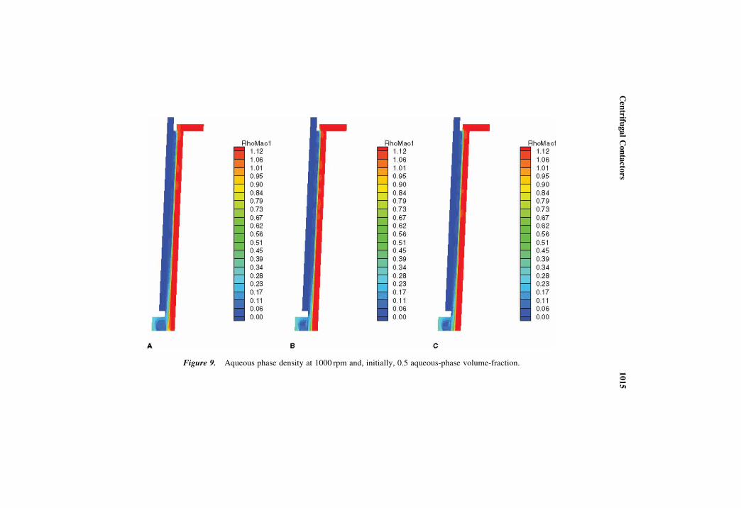
Figure 9. Aqueous phase density at 1000 rpm and, initially, 0.5 aqueous-phase volume-fraction.
Centrifu
galContacto
rs1015

Figure 10. Aqueous-phase density at 3000 rpm and, initially, 0.5 aqueous-phase volume-fraction.
N.T.Padial-C
ollin
set
al.
1016
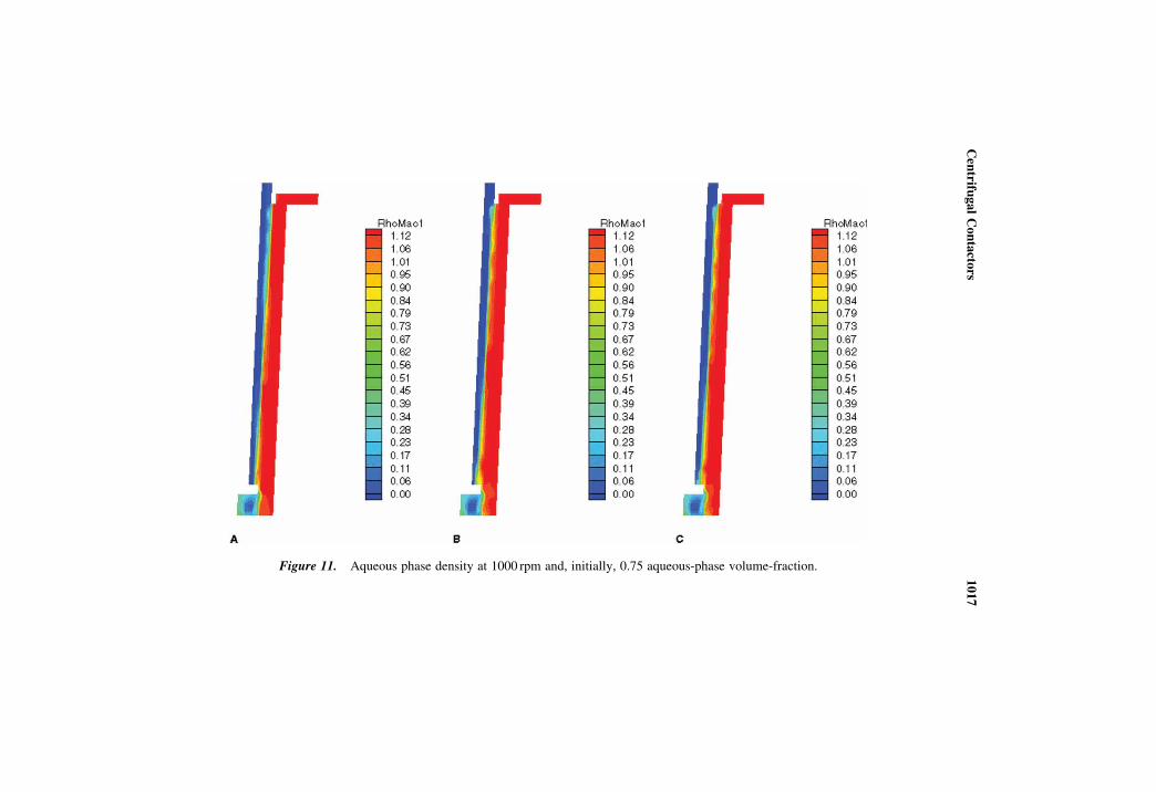
Figure 11. Aqueous phase density at 1000 rpm and, initially, 0.75 aqueous-phase volume-fraction.
Centrifu
galContacto
rs1017

Figure 12. Aqueous phase density at 3000 rpm and, initially, 0.75 aqueous phase volume fraction.
N.T.Padial-C
ollin
set
al.
1018

Figure 13. 3D results for the aqueous phase density after an initial mixture
with 75% aqueous phase: a) 3D display; b) Cut at 458 of the results shown in
(a).
Centrifu
galContacto
rs1019

Figure 14. Steady-state heavy-species mass-fraction in the aqueous-phase
at 3000 rpm.
N.T.Padial-C
ollin
set
al.
1020

Figure 15. Steady-state heavy-species mass-fraction in the aqueous-phase at
1000 rpm.
Centrifu
galContacto
rs1021

For the rotation zone at 3000 rpm, we see much better mass transfer for
the inclined device. This does not seem to be the case for the zone at
1000 rpm as we see in Figure 15.
CONCLUSIONS
We have solved the momentum and mass conservation equations in the simu-
lation of the separation of the aqueous and the organic components in the rotor
zone of a centrifugal contactor.We have demonstrated a computational scheme
and a tool which can be used to examine complex hydraulics, to explore effects
of the geometry in the process, and to study the influence of different initial
conditions, distinct rotor speeds, and diverse physical contributions. We
have studied the importance of the effective viscosity. Its effect seems
important at the low and high angular velocities, especially, for the vertical
contactor case. Since the objective is to reach very high extraction-efficiency,
the more accuracy in the modeling of effective viscosity in the simulations
may be necessary. The calculations also show a potentially strong effect
from mass transfer on the dynamics, indicating the need for realistic mass
transfer parameters before more definitive statements can be made.
Ultimately, these simulations aim at improving the efficiency of the cen-
trifugal contactors by allowing, for example, investigation of alternative
shapes for the devices or suggesting more appropriate initial conditions. Both
of these had significant effects in our simulations. Future plans include the evalu-
ation and optimization of advanced designs for contactors as well the investi-
gation of the issue of scale to determine the minimum size for pilot units.
REFERENCES
1. Berstein, G.J., Grosvenor, D.E., Lenc, J.F., and Levitz, N.M. (1973) A high-capacity annular centrifugal contactor. Nucl. Tech., 20: 200–202.
2. Leonard, R.A., Bernstein, G.J., Ziegler, A.A., and Pelto, R.H. (1980) Annular cen-trifugal contactors for solvent extraction. Sep. Sci. Technol., 15: 925–943.
3. Leonard, R.A., Pelto, R.H., Zeigler, A.A., and Bernstein, G.J. (1980) Flow overcircular wires in a centrifugal field. Can. J. Chemical Eng., 58 (4): 531–534.
4. Leonard, R.A. (1988) Recent advances in centrifugal contactor design. Sep. Sci.Technol., 23: 1473–1487.
5. Leonard, R.A. (1987) Use of electronic worksheets for calculation of stagewisesolvent extraction processes. Sep. Sci. Technol., 22 (2&3): 535–556.
6. Leonard, R.A. and Regalbuto, M.C. (1994) Spreadsheet algorithm for stagewisesolvent extraction. Solvent Extraction and Ion Exchange, 12 (5): 909–930.
7. Wallwork, A.L., Denniss, I.S., Taylor, R.J., Bothwell, P., Birkett, J.E., andBaker, S. (1999) Modelling of advanced flow sheets using data from miniaturecontactor trials. Nuclear Energy, 38 (1): 31–35.
8. Leonard, R.A., Bernstein, G.J., Pelto, R.H., and Zeigler, A.A. (1981) Liquid–liquid dispersion in turbulent Couette flow. AIChE Journal, 27 (3): 495–503.
N. T. Padial-Collins et al.1022

9. Renardy, Y. and Joseph, D.D. (1985) Couette flow of two fluids between con-centric cylinders. J. Fluid Mech., 150: 381–394.
10. Baier, G. and Graham, M.D. (1998) Two-fluid Taylor-Couette flow: Experimentsand linear theory for immiscible liquids between corotating cylinders. Phys.Fluids, 10 (12): 3045–3053.
11. VanderHeyden, W.B., Dendy, E.D., and Padial-Collins, N.T. (2002) CartaBlanca-Apure-Java, component-based systems simulation tool for coupled nonlinear physicson unstructured grids–an update. Concurrency and Computat: Pract. Exper., 14:1–28.
12. Meikrantz, D.H., Macaluso, L.L., Heald, C.J., Mendoza, G., and Meikrantz, S.B.(2002) A new annular centrifugal contactor for pharmaceutical process. Chem.Eng. Comm., 189 (12): 1629–1639.
13. See, for example, specifications for Agricultural Products Centrifugal Contactorsin http://www.rousselet-robatel.com/products/lx.php.
14. White, F.M. (1974) Viscous Fluid Flow; McGraw Hill: NY.15. Yarbro, S.L. and Schreiber, S.B. (2003) Using process intensification in the
actinide processing industry. J. Chem. Technol. Biotechnol., 78: 254–259.16. Boycott, A.E. (1920) Sedimentation of blood corpuscles. Nature, 104: 532.17. (a) Einstein, A. (1906) A new determination of molecular dimensions. Ann. Phys.,
19: 289–306; (b) Einstein, A. (1911) The theory of the Brownian movement. Ann.Phys., 1911, 34: 591–592.
18. Arrhenius, S. (1917) The viscosity of solutions. Biochem. J., 11: 112–133.19. Eilers, H. (1941) Die Viskositat von Emulsionen hochviskoser Stoffe als Funktion
der Konzentration. Kolloid Z., 97: 313–321.20. Mooney, M. (1951) The viscosity of a concentrated suspension of spherical
particles. J. Colloid. Sci., 6: 162–170.21. Rutgers, I.R. (1962) Relative viscosity and concentration. Rheol. Acta, 2:
305–348.22. Thomas, D.G. (1965) Transport characteristics of suspensions. J. Colloid. Sci., 20:
267–277.23. Frankel, N.A. and Acrivos, A. (1967) On the viscosity of concentrated suspension
of solid spheres. Chem. Eng. Sci., 22: 847–853.24. Barnes, H.A., Hutton, J.F., and Walters, K. (1989) An Introduction to Rheology;
Elsevier: Amsterdam, The Netherlands.25. Cheng, N.S. and Law, W.K.A. (2003) Exponential formula for computing effective
viscosity. Powder Technology, 129: 156–160.26. Hsueh, C.-H. and Becher, P.F. (2005) Effective viscosity of suspensions of
spheres. J. Am. Ceram. Soc., 88 (4): 1046–1049.27. Selker, A., Sleicher, C.A., Jr. (1965) Factors affecting which phase will disperse
when immiscible liquids are stirred together. Can. J. Chem. Eng., 43 (6): 298–301.28. Nadler, M., Mewes, D. (1997) Flow induced emulsification in the flow of two
immiscible liquids in horizontal pipes. Int. J. Multiphase Flow, 23 (1): 55–68.29. Brauner, N. and Ullmann, A. (2002) Modeling of phase inversion phenomenon in
two-phase pipe flows. Int. J. Multiphase Flow, 28: 1177–1204.30. Lhuillier, D. (2003) Dynamics of interfaces and rheology of immiscible liquid–
liquid mixtures. C. R. Mecanique, 331: 113–118.31. Ioannou, K. and Jorgen, Nydal O.Angeli, P. (2005) Phase inversion in dispersed
liquid–liquid flows. Exp. Therm. Fluid Sci., 29: 331–339.
Centrifugal Contactors 1023