Embed Size (px)
Citation preview
Centre d’Analyse Théorique et de
Traitement des données économiques
Center for the Analysis of Trade
and economic Transitions
CATT-UPPA
Collège Sciences Sociales et Humanités (SSH)
Droit, Economie, Gestion
Avenue du Doyen Poplawski - BP 1633
64016 PAU Cedex - FRANCE
Tél. (33) 5 59 40 80 61/62
Internet : http://catt.univ-pau.fr/live/
CATT WP No. 9
July 2019
POTENTIAL EFFECTS OF
SCALING-UP INFRASTRUCTURE
IN PERU :
A GENERAL EQUILIBRIUM
MODEL-BASED ANALYSIS
Jorge DAVALOS
Jean-Marc MONTAUD
Nicolas PECASTAING
1
Potential effects of scaling-up infrastructure in Peru: a general equilibrium
model-based analysis
Abstract
This study assesses the potential economic impacts of investments dedicated to filling
infrastructure gaps in Peru. By using a national database at the firm level, we start by
empirically estimating the positive externalities of Peruvian infrastructure on private activities’
output. In the second step, these estimates are introduced in a dynamic Computable General
Equilibrium model used to conduct counterfactual simulations of various investment plans in
infrastructure over a 15-year period. These simulations show to what extent scaling-up
infrastructure could be a worthwhile strategy to achieve economic growth in Peru; however,
they also show that these benefits depend on the choice of funding schemes related to such
public spending.
Keywords: Infrastructure, Productivity, CGE model, Peru
JEL classification: H54, O47, D58
Jorge Dávalos
UNIVERSIDAD DEL PACÍFICO, CENTRO DE INVESTIGACIÓN DE LA UNIVERSIDAD
DEL PACIFICO (CIUP)
Postal address: Av. Salaverry 2020, Jesús maría, Lima 11, Perú.
E-mail: [email protected]
Jean-Marc Montaud UNIV PAU & PAYS ADOUR, CENTRE D'ANALYSE THEORIQUE ET DE
TRAITEMENT DES DONNEES ECONOMIQUES, EA753
Postal address: Collège EEI, 8 Allée des Platanes, 64100, Bayonne France
E-mail: [email protected]
Nicolas Pécastaing
UNIVERSIDAD DEL PACÍFICO, CENTRO DE INVESTIGACIÓN DE LA UNIVERSIDAD
DEL PACIFICO (CIUP)
Postal address: Av. Salaverry 2020, Jesús maría, Lima 11, Perú.
E-mail: [email protected]
2
1. Introduction
Over the last decade, public investments in infrastructure have significantly increased in
Peru while the country benefited from the windfall revenues of the commodity prices’ boom.
However, current levels of Peruvian infrastructure remain insufficient with major deficits areas
including economic assets such energy, telecommunications, and transportation facilities or
social infrastructure such water and sanitation, health, or education (AFIN, 2015; ECLAC,
2015a; Sánchez et al., 2017). Although maintaining a high level of investments dedicated to
filling these gaps might be difficult for the next years with the likely adverse fiscal
consequences of the end of the commodity super cycle (Werner and Santos, 2015), many studies
advocate that such investments should not be neglected despite these new unfavourable
conditions. In the short term, they might represent an alternative engine for growth; in a longer
term, they might also contribute to breaking some bottlenecks often cited as impediments to
development of this country (Kohli and Basil 2011; IMF, 2014, CEPLAN, 2011, 2015; IMF,
2016; Fay et al., 2017; Sánchez et al, 2017). In this context, the main objective of this study is
to value the potential effects that investing in scaling-up infrastructure could generate on
Peruvian economic performance.
We follow many studies in the economic literature which consider that public infrastructural
assets are critical features for developing countries such as Peru and which highlight various
direct or indirect links between infrastructure stocks (or their variations) and growth or other
development outcomes (for comprehensive surveys, see e.g. Estache, 2006; Romp and de Haan,
2007; Straub, 2008, 2011). However, while the majority of this literature uses partial
equilibrium or macro level empirical approaches, we preferred to use a dynamic Computable
General Equilibrium (CGE) model to numerically simulate the potential impacts of various
multi-annual public investment plans in infrastructure in Peru. According to our knowledge,
such an applied economy-wide Walrassian framework has never been used for these purposes
in this country (see e.g. IMF, 2016 for a survey) even if it can be a useful complement to partial
equilibrium constructs or pure empirical analyses. By addressing the complexity of a market-
driven economy and capturing various feedback effects among prices, supply, demand, and
income, CGE modelling can provide a substantial understanding of the multiple micro-macro
links through public spending on new infrastructure may affect an economy. In this spirit, in
addition to the common short-term multiplier or crowding-on effects usually captured in
models, some recent CGE studies drawing on growth theory have for instance introduced the
positive externalities that public spending on new infrastructure can generate on private
3
activities’ output (see e.g. Rioja, 2001; Adam and Bevan, 2006; Estache et al., 2012; Cockburn
et al., 2013; Boccanfuso et al., 2014; Borojo, 2015; Chitiga et al. 2016; Mbanda and Chitiga,
2017). However, these studies have rarely valued these critical parameters accurately and often
take them from the extant empirical literature which has considerably grown up since the
seminal works of Aschauer (1989) or Munnell (1992). But estimates display large variations
across studies due to differences in the definitions of infrastructure; type of output measures
used as dependent variables; econometric specifications and sample coverage; or whether
endogeneity and stationarity concerns are properly addressed (see e.g. Bom and Ligthart, 2014
or Sanchez et al., 2017 for a global review and Vasquez, 2008, Urrunaga and Aparicio, 2012,
or Machado and Toma, 2017 for Peruvian specific analyses). Accordingly, following this
research stream, we introduce such externalities in our CGE model for Peru but we make our
own estimates of these potential supply effects of infrastructure by using a national firm
database provided by the Peruvian National Statistical Institute (INEI).
Section 2 details the main features of the dynamic CGE model and section 3 describes the
empirical strategy that we use to quantify the private output elasticities of public infrastructure
in Peru. Section 4 details the results of simulations of various scenarios of public investment
plans dedicated to scaling-up infrastructure in the country over a 15-year period. Finally, section
5 concludes and provides suggestions for further research.
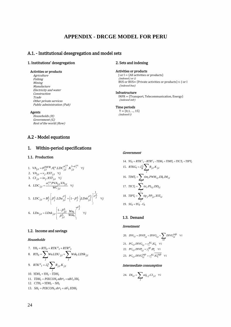
2. General equilibrium modelling framework
Our CGE model is relatively aggregated and features one household, one government agent,
eight private activities, and one non-merchant activity. This model is mainly adapted from the
PEP 1-t model of Decaluwé et al. (2013) and relies on fairly standard assumptions of dynamic
general equilibrium analysis (equations and variables are provided in the Appendix).
Regarding the within-period specifications of the model, on the supply side, each producer
maximises its profit by combining skilled and unskilled labour with fixed capital (Eq. 1–6). On
the income side, each agent receives factor revenues on the basis of its initial endowments and
transfer income from other agents (Eq. 7–19). On the demand side, intermediate consumption
is driven by fixed technical coefficients in production processes (Eq. 24); households’
consumption follows a linear expenditure system function derived from utility maximisation
behaviours (Eq. 26); government’s consumption is supposed to be exogenous; and demands for
investment purposes are derived from nominal investments and distributed among commodities
4
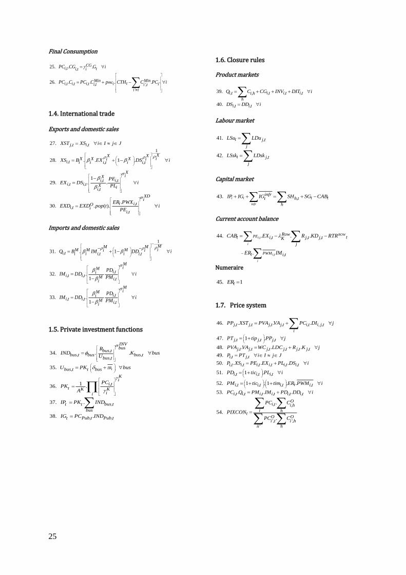
in fixed shares (Eq. 20-23). On the product’s market, each good can be sold locally or abroad
given a Constant Elasticity Transformation specification (Eq. 27–30). The domestic goods are
assumed to be imperfectly substitutable with imported products, given an Armington
specification (Eq. 31–33). Prices of domestic goods are determined endogenously to equilibrate
supply and demand (Eq. 39–40). On the labour market, the skilled and unskilled overall labour
forces are fixed, and workers can flow freely across all activities with wage rates determined
endogenously (Eq. 41–42). Finally, nominal investments are savings driven on the capital
market, and the nominal exchange rate is chosen as the numeraire for the economy (Eq. 44–
45).
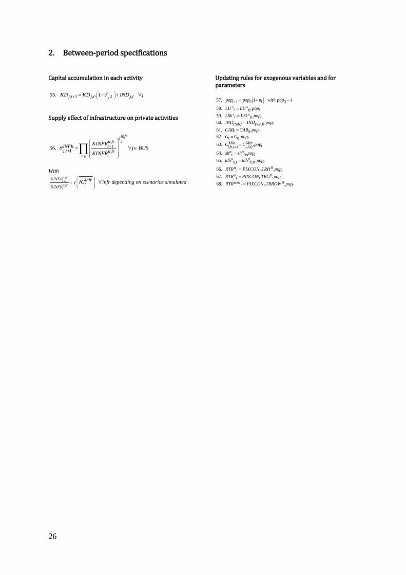
Regarding the between-period specifications of the model, we consider a dynamic recursive
framework which means that agents’ behaviours are based on adaptive expectations rather than
on forward-looking expectations. A main specification pertains to the accumulation of capital
in each activity (Eq. 55), which reflects an exogenous depreciation rate and the volume of new
capital installed as determined in the preceding period. In the public sector, the latter is
supposed to be given. In private activities, it is derived from an investment demand function
and allocated in a putty-clay fashion across sectors in accordance with returns to investment
(Eq. 34–38).
How we introduced infrastructure topics in the model deserves more attention. Following
recent CGE studies (e.g. Estache et al., 2012 or Boccanfuso et al., 2014), we linked in a Hicks’s
neutral manner the total factor productivity of Peruvian private activities to the stocks of public
infrastructure in the country (Eq. 1 and 56). For a given period t, the value added of each private
activity is derived from a standard Cobb-Douglas technology combining labour and capital but
also depends on a parameter which reflects the supply effect of infrastructure on the activity’s
performances. This parameter is time-variant and can increase with exogenous public
investments dedicated to scaling-up infrastructure.
On these bases, the model is used to generate time paths for the evolution of Peruvian
economic variables by numerical simulation of successive general equilibriums under different
scenarios of multi-annual investment plans in infrastructure. For a given period t, a general
equilibrium of the model is defined by the vector of prices and wages for which demand equals
supply in all markets simultaneously. All things being equal, such investments are expected to
produce three combined effects. First, by increasing the demand for the activities which produce
the capital goods required for scaling-up infrastructure, they could generate a multiplier effect
on the economy and, therefore, upward pressure on demand and prices on product markets.
Second, given the savings-investment constraint which drives the capital market’s equilibrium
5
in the model, and which thus determines how much savings are taken up by public investment,
they could generate a crowding-out effect for other investments for non-infrastructural
purposes. Third, by changing the nature of production processes in private activities in a Hicks’s
neutral manner, they finally could also generate a supply effect leading to productivity
increases, capital rental rate variations (and therefore to re-allocation of private investments
across activities), and producer price reductions.
To define an initial general equilibrium of the economy and to calibrate the CGE model
parameters, we used Peru’s 2014 Social Accounting Matrix, the most recent data available for
the country (Ministry of Production, 2016). When such calibrations were not possible, we
obtained the parameters from extant literature, including CGE models that have been
established for Peru. However, the calibration of the production functions of private activities
deserves more attention. Because of their critical role in the model, we econometrically estimate
their parameters.
3. Estimates of private output contributions of public infrastructure in Peru
In the economic literature, most of the analyses use a function primal approach to estimate
the effects of exogenous variations of infrastructure on activities’ productivity and consider the
stock of infrastructure as an additional input in production functions at the aggregated or sector
levels. Other studies use a dual approach by estimating a cost function which threats public
infrastructure as an unpaid factor of production. A few other studies use non-parametrical
models considering non-linearities in the functional relationship of the production technology
(see e.g. Bom and Ligthart, 2014). Consistent with our macroeconomic CGE modelling, we use
a primal approach at a disaggregated sector level. Data for economic activities are found in the
national firm database created by the INEI from 2004–2015 on the bases of its annual economic
survey (Encuesta Economica Annual, EEA). From the statements of each firm recorded in this
survey (almost 60,000 firms), we determine their belonging sector, value added, labour force,
and capital stock. For the latter, we use two alternative approaches, specific to small and
medium to big firms. For small firms, the capital stock is proxied by the total fixed assets as
reported on their general balance sheet. For a medium to big firm, which tends to include
financial investments not involved in the productive process as fixed assets, it is proxied by the
value of the stock of equipment.
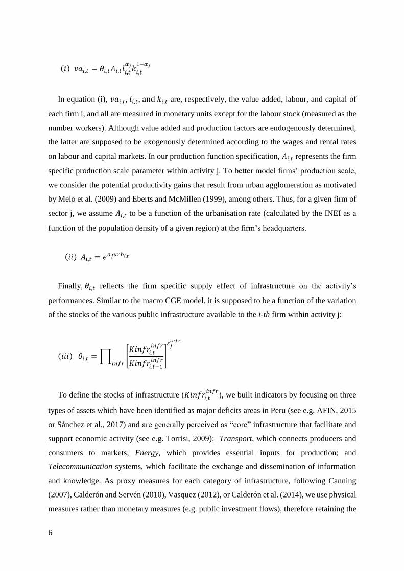
On these bases, for each firm i, pertaining to each activity j, we assume a sector-specific
production technology with a value added at time t following a Cobb-Douglas specification:
6
(𝑖) 𝑣𝑎𝑖,𝑡 = 𝜃𝑖,𝑡𝐴𝑖,𝑡𝑙𝑖,𝑡
𝛼𝑗𝑘𝑖,𝑡
1−𝛼𝑗
In equation (i), 𝑣𝑎𝑖,𝑡, 𝑙𝑖,𝑡, and 𝑘𝑖,𝑡 are, respectively, the value added, labour, and capital of
each firm i, and all are measured in monetary units except for the labour stock (measured as the
number workers). Although value added and production factors are endogenously determined,
the latter are supposed to be exogenously determined according to the wages and rental rates
on labour and capital markets. In our production function specification, 𝐴𝑖,𝑡 represents the firm
specific production scale parameter within activity j. To better model firms’ production scale,
we consider the potential productivity gains that result from urban agglomeration as motivated
by Melo et al. (2009) and Eberts and McMillen (1999), among others. Thus, for a given firm of
sector j, we assume 𝐴𝑖,𝑡 to be a function of the urbanisation rate (calculated by the INEI as a
function of the population density of a given region) at the firm’s headquarters.
(𝑖𝑖) 𝐴𝑖,𝑡 = 𝑒𝑎𝑗𝑢𝑟𝑏𝑖,𝑡
Finally, 𝜃𝑖,𝑡 reflects the firm specific supply effect of infrastructure on the activity’s
performances. Similar to the macro CGE model, it is supposed to be a function of the variation
of the stocks of the various public infrastructure available to the i-th firm within activity j:
(𝑖𝑖𝑖) 𝜃𝑖,𝑡 = ∏ [𝐾𝑖𝑛𝑓𝑟𝑖,𝑡
𝑖𝑛𝑓𝑟
𝐾𝑖𝑛𝑓𝑟𝑖,𝑡−1𝑖𝑛𝑓𝑟
]
𝜀𝑗𝑖𝑛𝑓𝑟
𝐼𝑛𝑓𝑟
To define the stocks of infrastructure (𝐾𝑖𝑛𝑓𝑟𝑖,𝑡𝑖𝑛𝑓𝑟
), we built indicators by focusing on three
types of assets which have been identified as major deficits areas in Peru (see e.g. AFIN, 2015
or Sánchez et al., 2017) and are generally perceived as “core” infrastructure that facilitate and
support economic activity (see e.g. Torrisi, 2009): Transport, which connects producers and
consumers to markets; Energy, which provides essential inputs for production; and
Telecommunication systems, which facilitate the exchange and dissemination of information
and knowledge. As proxy measures for each category of infrastructure, following Canning
(2007), Calderón and Servén (2010), Vasquez (2012), or Calderón et al. (2014), we use physical
measures rather than monetary measures (e.g. public investment flows), therefore retaining the
7
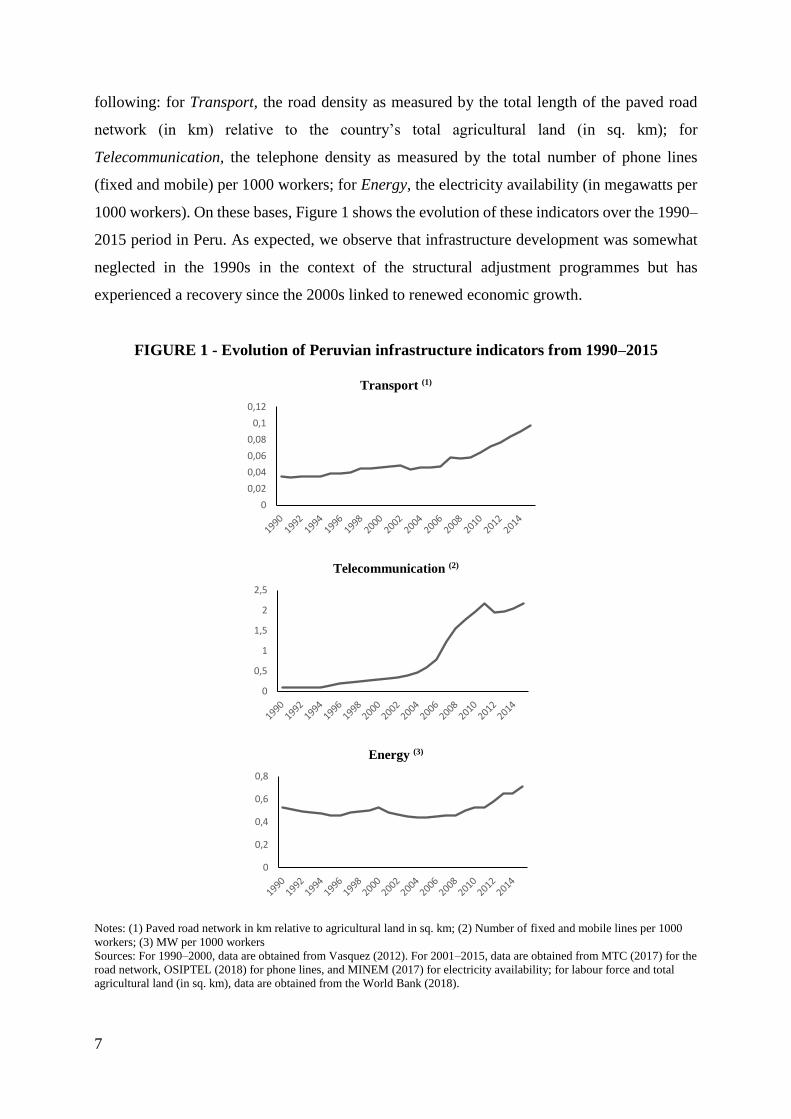
following: for Transport, the road density as measured by the total length of the paved road
network (in km) relative to the country’s total agricultural land (in sq. km); for
Telecommunication, the telephone density as measured by the total number of phone lines
(fixed and mobile) per 1000 workers; for Energy, the electricity availability (in megawatts per
1000 workers). On these bases, Figure 1 shows the evolution of these indicators over the 1990–
2015 period in Peru. As expected, we observe that infrastructure development was somewhat
neglected in the 1990s in the context of the structural adjustment programmes but has
experienced a recovery since the 2000s linked to renewed economic growth.
FIGURE 1 - Evolution of Peruvian infrastructure indicators from 1990–2015
Transport (1)
Telecommunication (2)
Energy (3)
Notes: (1) Paved road network in km relative to agricultural land in sq. km; (2) Number of fixed and mobile lines per 1000
workers; (3) MW per 1000 workers
Sources: For 1990–2000, data are obtained from Vasquez (2012). For 2001–2015, data are obtained from MTC (2017) for the
road network, OSIPTEL (2018) for phone lines, and MINEM (2017) for electricity availability; for labour force and total
agricultural land (in sq. km), data are obtained from the World Bank (2018).
0
0,02
0,04
0,06
0,08
0,1
0,12
0
0,5
1
1,5
2
2,5
0
0,2
0,4
0,6
0,8
8
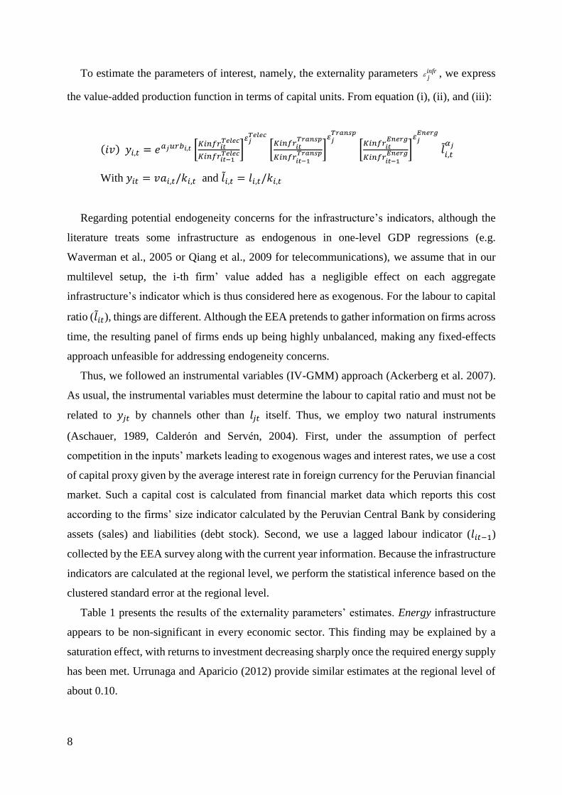
To estimate the parameters of interest, namely, the externality parameters infrj
, we express
the value-added production function in terms of capital units. From equation (i), (ii), and (iii):
(𝑖𝑣) 𝑦𝑖,𝑡 = 𝑒𝑎𝑗𝑢𝑟𝑏𝑖,𝑡 [𝐾𝑖𝑛𝑓𝑟𝑖𝑡
𝑇𝑒𝑙𝑒𝑐
𝐾𝑖𝑛𝑓𝑟𝑖𝑡−1𝑇𝑒𝑙𝑒𝑐]
𝜀𝑗𝑇𝑒𝑙𝑒𝑐
[𝐾𝑖𝑛𝑓𝑟𝑖𝑡
𝑇𝑟𝑎𝑛𝑠𝑝
𝐾𝑖𝑛𝑓𝑟𝑖𝑡−1𝑇𝑟𝑎𝑛𝑠𝑝]
𝜀𝑗𝑇𝑟𝑎𝑛𝑠𝑝
[𝐾𝑖𝑛𝑓𝑟𝑖𝑡
𝐸𝑛𝑒𝑟𝑔
𝐾𝑖𝑛𝑓𝑟𝑖𝑡−1𝐸𝑛𝑒𝑟𝑔]
𝜀𝑗𝐸𝑛𝑒𝑟𝑔
𝑙𝑖,𝑡
𝛼𝑗
With 𝑦𝑖𝑡 = 𝑣𝑎𝑖,𝑡/𝑘𝑖,𝑡 and 𝑙𝑖,𝑡 = 𝑙𝑖,𝑡/𝑘𝑖,𝑡
Regarding potential endogeneity concerns for the infrastructure’s indicators, although the
literature treats some infrastructure as endogenous in one-level GDP regressions (e.g.
Waverman et al., 2005 or Qiang et al., 2009 for telecommunications), we assume that in our
multilevel setup, the i-th firm’ value added has a negligible effect on each aggregate
infrastructure’s indicator which is thus considered here as exogenous. For the labour to capital
ratio (𝑙𝑖𝑡), things are different. Although the EEA pretends to gather information on firms across
time, the resulting panel of firms ends up being highly unbalanced, making any fixed-effects
approach unfeasible for addressing endogeneity concerns.
Thus, we followed an instrumental variables (IV-GMM) approach (Ackerberg et al. 2007).
As usual, the instrumental variables must determine the labour to capital ratio and must not be
related to 𝑦𝑗𝑡 by channels other than 𝑙𝑗𝑡 itself. Thus, we employ two natural instruments
(Aschauer, 1989, Calderon and Serven, 2004). First, under the assumption of perfect
competition in the inputs’ markets leading to exogenous wages and interest rates, we use a cost
of capital proxy given by the average interest rate in foreign currency for the Peruvian financial
market. Such a capital cost is calculated from financial market data which reports this cost
according to the firms’ size indicator calculated by the Peruvian Central Bank by considering
assets (sales) and liabilities (debt stock). Second, we use a lagged labour indicator (𝑙𝑖𝑡−1)
collected by the EEA survey along with the current year information. Because the infrastructure
indicators are calculated at the regional level, we perform the statistical inference based on the
clustered standard error at the regional level.
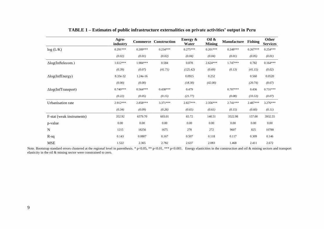
Table 1 presents the results of the externality parameters’ estimates. Energy infrastructure
appears to be non-significant in every economic sector. This finding may be explained by a
saturation effect, with returns to investment decreasing sharply once the required energy supply
has been met. Urrunaga and Aparicio (2012) provide similar estimates at the regional level of
about 0.10.
9
TABLE 1 – Estimates of public infrastructure externalities on private activities’ output in Peru
Note. Bootstrap standard errors clustered at the regional level in parenthesis. * p<0.05, ** p<0.01, *** p<0.001. Energy elasticities in the construction and oil & mining sectors and transport
elasticity in the oil & mining sector were constrained to zero.
Agro-
industry Commerce Construction
Energy &
Water
Oil &
Mining Manufacture Fishing
Other
Services
log (L/K) 0.291*** 0.209*** 0.234*** 0.275*** 0.201*** 0.248*** 0.267*** 0.254***
(0.02) (0.01) (0.02) (0.04) (0.04) (0.01) (0.05) (0.01)
Δlog(Inftelecom.) 1.612*** 1.984*** 0.584 0.878 2.624*** 1.747*** 0.782 0.164***
(0.39) (0.07) (41.71) (125.42) (0.69) (0.13) (41.15) (0.02)
Δlog(InfEnergy) 8.33e-32 1.24e-16 0.0915 0.252 0.560 0.0520
(0.00) (0.00) (18.30) (42.00) (20.74) (8.67)
Δlog(InfTransport) 0.740*** 0.564*** 0.438*** 0.479 0.707*** 0.436 0.731***
(0.22) (0.05) (0.15) (21.77) (0.08) (33.53) (0.07)
Urbanisation rate 2.912*** 2.858*** 3.371*** 2.827*** 2.356*** 2.741*** 2.487*** 3.276***
(0.34) (0.09) (0.26) (0.65) (0.61) (0.15) (0.60) (0.11)
F-stat (weak instruments) 352.92 6579.70 603.01 65.72 140.51 3522.98 157.00 3932.55
p-value 0.00 0.00 0.00 0.00 0.00 0.00 0.00 0.00
N 1215 18256 1675 278 272 9607 825 10788
R-sq 0.143 0.0807 0.167 0.507 0.118 0.117 0.309 0.146
MSE 1.522 2.365 2.782 2.637 2.083 1.468 2.411 2.672
10
Although the estimates were significant, they were estimated with respect to regional
economies and corresponded to a period (1980–2009) where energy supply was a binding
constraint to economic growth. By contrast, the Transport externality parameter tends to exhibit
significant results ranging from 0.44 to 0.74, and all are statistically significant except for the
oil & mining and energy & water sectors. Externality parameters for Telecommunication exhibit
heterogeneous results across the economic sectors, from non-significant in construction, energy
& water, and fishing to highly statistically significant magnitudes in oil & mining, commerce,
and manufacturing. The high heterogeneity of the elasticity parameters (from non-significant
to significant and greater than one) may be explained by the literature. From the data of single
and multiple countries, Waverman et al. (2005) and Qiang et al. (2009) have observed that the
telecommunications effects decrease with the penetration rate, that is, greater effects are
associated with lower penetration rates. Regarding the validity (weakness) of our instruments,
the F-statistics that assess their joint significance are highly significant and greater than 10
(instrument weakness rule of thumb).
4. Simulating investment plans to fill Peruvian infrastructural gaps
4.1 Definition of scenarios
We deliberately set a relatively short time horizon (15-year period) for the different
investment scenarios to exclude potential significant structural changes in the Peruvian
economy and, thus, maintain the consistency of the parameters’ initial calibration of the CGE
model. Following the standard procedure commonly used in dynamic CGE modelling, we first
define a Business as usual (BAU) scenario by updating various constants and exogenous
variables from one year to the next (Eq. 57–68) by using the annual population growth rate
which is projected to be close to 1.1% over the period set by the INEI (2009). Second, we
conduct ex-ante counterfactual experiments by comparing the outcome of simulations of
different investment plans in infrastructure with those of the BAU scenario.
Our first group of scenario refers to vertical gaps in the infrastructure of Peru compared with
the demand generated by its economic activity (Perrotti and Sánchez, 2011). The latter are
estimated by AFIN (2015) for various infrastructural assets by using the methodology proposed
by Fay and Yepes (2003). Their results show that Peru should invest USD 13.4 billion in
telecommunications and USD 6.9 billion in its road network to fill its gaps. A lower investment
11
level is required for Energy (USD 1.5 billion) because of the current significantly high supply
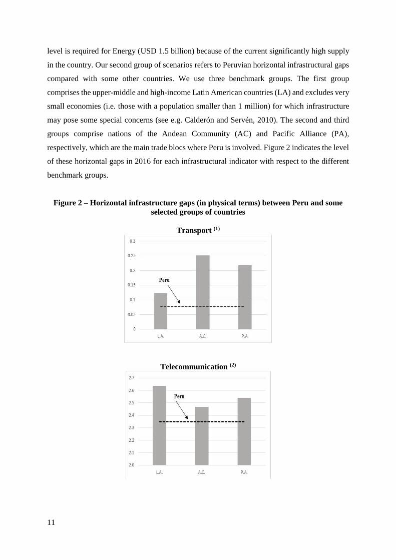
in the country. Our second group of scenarios refers to Peruvian horizontal infrastructural gaps
compared with some other countries. We use three benchmark groups. The first group
comprises the upper-middle and high-income Latin American countries (LA) and excludes very
small economies (i.e. those with a population smaller than 1 million) for which infrastructure
may pose some special concerns (see e.g. Calderón and Servén, 2010). The second and third
groups comprise nations of the Andean Community (AC) and Pacific Alliance (PA),
respectively, which are the main trade blocs where Peru is involved. Figure 2 indicates the level
of these horizontal gaps in 2016 for each infrastructural indicator with respect to the different
benchmark groups.
Figure 2 – Horizontal infrastructure gaps (in physical terms) between Peru and some
selected groups of countries
Transport (1)
Telecommunication (2)
12
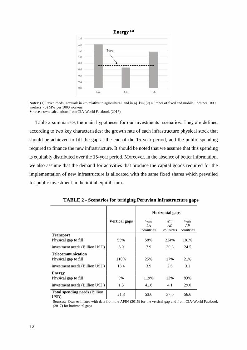
Energy (3)
Notes: (1) Paved roads’ network in km relative to agricultural land in sq. km; (2) Number of fixed and mobile lines per 1000
workers; (3) MW per 1000 workers
Sources: own calculations from CIA-World Factbook (2017)
Table 2 summarises the main hypotheses for our investments’ scenarios. They are defined
according to two key characteristics: the growth rate of each infrastructure physical stock that
should be achieved to fill the gap at the end of the 15-year period, and the public spending
required to finance the new infrastructure. It should be noted that we assume that this spending
is equitably distributed over the 15-year period. Moreover, in the absence of better information,
we also assume that the demand for activities that produce the capital goods required for the
implementation of new infrastructure is allocated with the same fixed shares which prevailed
for public investment in the initial equilibrium.
TABLE 2 - Scenarios for bridging Peruvian infrastructure gaps
Vertical gaps
Horizontal gaps
With
LA
countries
With
AC
countries
With
AP
countries
Transport
Physical gap to fill 55% 58% 224% 181%
investment needs (Billion USD) 6.9 7.9 30.3 24.5
Telecommunication
Physical gap to fill 110% 25% 17% 21%
investment needs (Billion USD) 13.4 3.9 2.6 3.1
Energy
Physical gap to fill 5% 119% 12% 83%
investment needs (Billion USD) 1.5 41.8 4.1 29.0
Total spending needs (Billion
USD) 21.8 53.6 37,0 56.6
Sources: Own estimates with data from the AFIN (2015) for the vertical gap and from CIA-World Factbook
(2017) for horizontal gaps
13
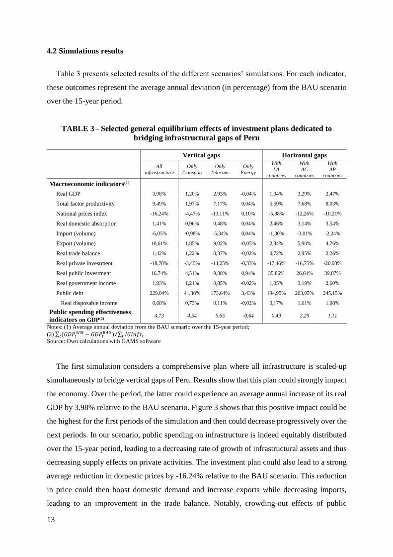
4.2 Simulations results
Table 3 presents selected results of the different scenarios’ simulations. For each indicator,
these outcomes represent the average annual deviation (in percentage) from the BAU scenario
over the 15-year period.
TABLE 3 - Selected general equilibrium effects of investment plans dedicated to
bridging infrastructural gaps of Peru
Vertical gaps Horizontal gaps
All
infrastructure
Only
Transport
Only
Telecom.
Only
Energy
With
LA countries
With
AC countries
With
AP countries
Macroeconomic indicators(1)
Real GDP 3,98% 1,20% 2,93% -0,04% 1,04% 3,29% 2,47%
Total factor productivity 9,49% 1,97% 7,17% 0,04% 5,59% 7,68% 8,03%
National prices index -16,24% -4,47% -13,11% 0,10% -5,88% -12,26% -10,21%
Real domestic absorption 1,41% 0,96% 0,48% 0,04% 2,46% 3,14% 3,54%
Import (volume) -6,05% -0,98% -5,34% 0,04% -1,30% -3,01% -2,24%
Export (volume) 10,61% 1,85% 9,02% -0,05% 2,84% 5,90% 4,76%
Real trade balance 1,42% 1,22% 0,37% -0,02% 0,72% 2,95% 2,26%
Real private investment -18,78% -3,45% -14,25% -0,33% -17,46% -16,75% -20,93%
Real public investment 16,74% 4,51% 9,88% 0,94% 35,86% 26,64% 39,87%
Real government income 1,93% 1,21% 0,85% -0,02% 1,05% 3,19% 2,60%
Public debt 229,04% 41,38% 173,64% 3,43% 194,95% 203,05% 245,15%
Real disposable income 0,68% 0,73% 0,11% -0,02% 0,17% 1,61% 1,08%
Public spending effectiveness
indicators on GDP(2) 4,73 4,54 5,65 -0,64 0,49 2,29 1,11
Notes: (1) Average annual deviation from the BAU scenario over the 15-year period;
(2) ∑ (𝐺𝐷𝑃𝑡𝑆𝐼𝑀
𝑡 − 𝐺𝐷𝑃𝑡𝐵𝐴𝑈) ∑ 𝐼𝐺𝐼𝑛𝑓𝑟𝑡𝑡⁄
Source: Own calculations with GAMS software
The first simulation considers a comprehensive plan where all infrastructure is scaled-up
simultaneously to bridge vertical gaps of Peru. Results show that this plan could strongly impact
the economy. Over the period, the latter could experience an average annual increase of its real
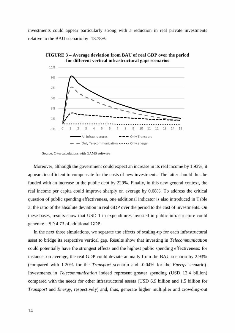
GDP by 3.98% relative to the BAU scenario. Figure 3 shows that this positive impact could be
the highest for the first periods of the simulation and then could decrease progressively over the
next periods. In our scenario, public spending on infrastructure is indeed equitably distributed
over the 15-year period, leading to a decreasing rate of growth of infrastructural assets and thus
decreasing supply effects on private activities. The investment plan could also lead to a strong
average reduction in domestic prices by -16.24% relative to the BAU scenario. This reduction
in price could then boost domestic demand and increase exports while decreasing imports,
leading to an improvement in the trade balance. Notably, crowding-out effects of public
14
investments could appear particularly strong with a reduction in real private investments
relative to the BAU scenario by -18.78%.
FIGURE 3 – Average deviation from BAU of real GDP over the period
for different vertical infrastructural gaps scenarios
Source: Own calculations with GAMS software
Moreover, although the government could expect an increase in its real income by 1.93%, it
appears insufficient to compensate for the costs of new investments. The latter should thus be
funded with an increase in the public debt by 229%. Finally, in this new general context, the
real income per capita could improve sharply on average by 0.68%. To address the critical
question of public spending effectiveness, one additional indicator is also introduced in Table
3: the ratio of the absolute deviation in real GDP over the period to the cost of investments. On
these bases, results show that USD 1 in expenditures invested in public infrastructure could
generate USD 4.73 of additional GDP.
In the next three simulations, we separate the effects of scaling-up for each infrastructural
asset to bridge its respective vertical gap. Results show that investing in Telecommunication
could potentially have the strongest effects and the highest public spending effectiveness: for
instance, on average, the real GDP could deviate annually from the BAU scenario by 2.93%
(compared with 1.20% for the Transport scenario and -0.04% for the Energy scenario).
Investments in Telecommunication indeed represent greater spending (USD 13.4 billion)
compared with the needs for other infrastructural assets (USD 6.9 billion and 1.5 billion for
Transport and Energy, respectively) and, thus, generate higher multiplier and crowding-out
-1%
1%
3%
5%
7%
9%
11%
0 1 2 3 4 5 6 7 8 9 10 11 12 13 14 15
All infrastructures Only Transport
Only Telecommunication Only energy
15
effects. Moreover, investments in Telecommunication also have higher supply effects in the
economy.
First, because the physical growth rate target for this infrastructural asset is higher (110%)
compared with other assets (55% and 5% for Transport and Energy, respectively). Second, as
shown in section 1, because Telecommunication infrastructure has higher positive average
externalities on private activities and affects a larger part of the Peruvian economy (88% of
total national private value added compared with 77.5% for Transport and even 0% for Energy).
Finally, three simulations show the potential impacts on the Peruvian economy of investment
plans dedicated to bridging its horizontal infrastructural gaps with respect to the different
benchmark groups retained in the scenarios. Results confirm those previously obtained for
vertical gaps. In each scenario, we observe that annual relative average real GDP increases,
domestic prices decrease, trade balance improves, private investments decrease, public debt
increases, or income per capita increases. However, the magnitude of these impacts is
differentiated between the scenarios because levels of public spending and allocations across
the different assets differ. For instance, filling infrastructural gaps with respect to nations of the
AC, which is the less-expensive scenario (USD 37.0 billion) and concerns mainly Transport,
(USD 30.3 billion, for a 224% growth rate achieved at the end of the period), could appear to
have the strongest effect on growth (+3.29%, relative to BAU) and, thus, higher public spending
effectiveness indicators. For the horizontal gap scenario with respect to LA, which represents
USD 53.6 billion mainly allocated to Energy (USD 41.8 billion), the relative impact on growth
could be only 1.04%. For the scenario with respect to the nations of the PA, which is the most
expensive (USD 56.6 billion, mainly allocated to Energy and Transport and achieving growth
rates of 83% and 181%, respectively, for these infrastructural assets), the average relative
annual growth deviation from BAU scenario could be 2.47%.
4.2 Alternative funding schemes for investments
In previous simulations, given the savings-investment constraint in the CGE model, new
public investments in infrastructure were implicitly supposed to be exclusively funded with
private saving (and public debt), generating strong crowding-out effects on private investments.
However, some CGE studies in the economic literature (see e.g. Boccanfuso et al., 2014)
demonstrate that in a general equilibrium framework, the choice of funding schemes related to
public spending is a key topic which could potentially affect the returns of new public
investments. Accordingly, we investigate three alternative funding options for previous
16
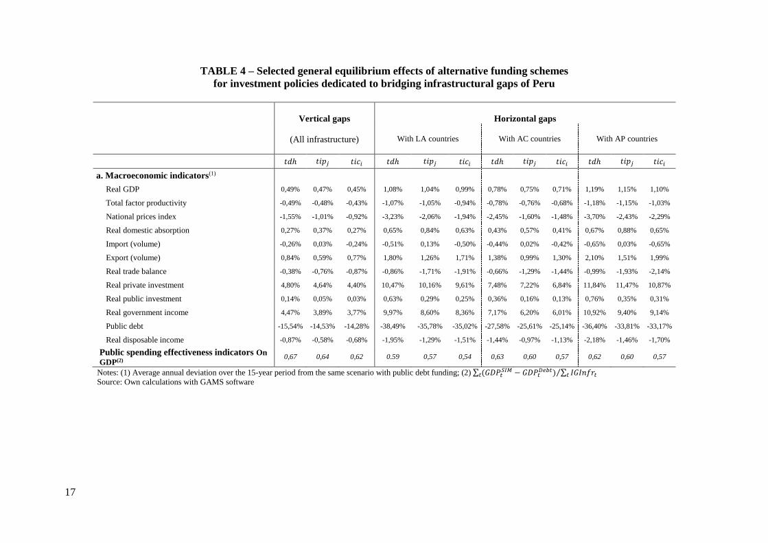
investments scenarios, namely, an increase in the households’ income tax rate (tdh), an increase
in production tax rates (tipj), and an increase in sale tax rates on commodities (tici). In each
case, the new levels of tax rates are determined to fully fund new investments. Results of the
simulations with these new funding schemes’ hypotheses are in Table 4. For an easier
comparison, the results are now presented as the relative deviation with the same scenario where
new infrastructure is funded with only public debt.
Whatever type of tax considered, it should be first noted that funding public investments
with additional taxes instead of private savings could significantly modify their potential
impacts, that is, it could particularly increase their positive effect on GDP and, thus, the public
spending effectiveness on the growth of such policies. For the vertical gaps scenario, the
average annual deviation of real GDP could, for instance, be close to +0.5% over the period,
compared with the same scenario with private savings funding. For horizontal gaps scenarios,
this deviation could be close to +1%. Using alternative funding schemes could also strengthen
the downward impacts on national prices of investment in new infrastructure. However, as
expected, the stronger deviations could be observed for the government income and public debt.
In the vertical gaps scenario, the former could be annually higher by close to +4%. This increase
could even be close to + 9%, 6%, and 10% for LA, AC and AP horizontal scenarios,
respectively. The public debt could be annually reduced by close to -15% in the vertical
scenario, and close to -35%, -26%, and -34% for the LA, AC, and AP horizontal scenarios,
respectively. Accordingly, the crowding-out effect on private investments could, therefore, be
strongly reduced (without, however, being cancelled). For the vertical gaps scenario, private
investments could be annually higher close to +4% over the period. For horizontal gaps
scenarios, private investments could be close to +10%, +7%, and +11% for the LA, AC, and
AP scenarios, respectively. However, in this new context, living conditions could degrade
sharply for Peruvian households, who would suffer, in all scenarios, an average decrease in
their income.
If we compare the simulation outcome of each type of tax, the results secondly show that the
income tax option seems to produce higher average deviation, although the differences are small
between alternative funding schemes. The main differences are observed for prices and
household income. For the income tax option, the increase in taxation decreases indeed directly
affects the income of households and, thus, their consumption and saving. For the production
tax and sales tax options, the effects are indirectly from increases in prices, which only reduces
the decreases induced by the supply effects of new infrastructure without fully compensating
them.
17
TABLE 4 – Selected general equilibrium effects of alternative funding schemes
for investment policies dedicated to bridging infrastructural gaps of Peru
Vertical gaps
(All infrastructure)
Horizontal gaps
With LA countries With AC countries With AP countries
𝑡𝑑ℎ 𝑡𝑖𝑝𝑗 𝑡𝑖𝑐𝑖 𝑡𝑑ℎ 𝑡𝑖𝑝𝑗 𝑡𝑖𝑐𝑖 𝑡𝑑ℎ 𝑡𝑖𝑝𝑗 𝑡𝑖𝑐𝑖 𝑡𝑑ℎ 𝑡𝑖𝑝𝑗 𝑡𝑖𝑐𝑖
a. Macroeconomic indicators(1)
Real GDP 0,49% 0,47% 0,45% 1,08% 1,04% 0,99% 0,78% 0,75% 0,71% 1,19% 1,15% 1,10%
Total factor productivity -0,49% -0,48% -0,43% -1,07% -1,05% -0,94% -0,78% -0,76% -0,68% -1,18% -1,15% -1,03%
National prices index -1,55% -1,01% -0,92% -3,23% -2,06% -1,94% -2,45% -1,60% -1,48% -3,70% -2,43% -2,29%
Real domestic absorption 0,27% 0,37% 0,27% 0,65% 0,84% 0,63% 0,43% 0,57% 0,41% 0,67% 0,88% 0,65%
Import (volume) -0,26% 0,03% -0,24% -0,51% 0,13% -0,50% -0,44% 0,02% -0,42% -0,65% 0,03% -0,65%
Export (volume) 0,84% 0,59% 0,77% 1,80% 1,26% 1,71% 1,38% 0,99% 1,30% 2,10% 1,51% 1,99%
Real trade balance -0,38% -0,76% -0,87% -0,86% -1,71% -1,91% -0,66% -1,29% -1,44% -0,99% -1,93% -2,14%
Real private investment 4,80% 4,64% 4,40% 10,47% 10,16% 9,61% 7,48% 7,22% 6,84% 11,84% 11,47% 10,87%
Real public investment 0,14% 0,05% 0,03% 0,63% 0,29% 0,25% 0,36% 0,16% 0,13% 0,76% 0,35% 0,31%
Real government income 4,47% 3,89% 3,77% 9,97% 8,60% 8,36% 7,17% 6,20% 6,01% 10,92% 9,40% 9,14%
Public debt -15,54% -14,53% -14,28% -38,49% -35,78% -35,02% -27,58% -25,61% -25,14% -36,40% -33,81% -33,17%
Real disposable income -0,87% -0,58% -0,68% -1,95% -1,29% -1,51% -1,44% -0,97% -1,13% -2,18% -1,46% -1,70%
Public spending effectiveness indicators On
GDP(2) 0,67 0,64 0,62 0.59 0,57 0,54 0,63 0,60 0,57 0,62 0,60 0,57
Notes: (1) Average annual deviation over the 15-year period from the same scenario with public debt funding; (2) ∑ (𝐺𝐷𝑃𝑡𝑆𝐼𝑀
𝑡 − 𝐺𝐷𝑃𝑡𝐷𝑒𝑏𝑡) ∑ 𝐼𝐺𝐼𝑛𝑓𝑟𝑡𝑡⁄
Source: Own calculations with GAMS software
18
5. Conclusion
In the current context of major infrastructure deficits, this study aimed to value the potential
outcome that scaling-up infrastructure could generate in Peru. First, using a microeconomic
database at the firm level, we empirically estimated the positive contribution of different types
of infrastructure on Peruvian private sectors. Our results show that, although energy
infrastructure has no significant effects on firms’ production, telecommunication infrastructure
exhibits highly significant externalities; similarly, road infrastructure’s contribution to
production is statistically significant across many economic activities. Second, numerical
simulations of investment plans over a 15-year period have been performed with a CGE model
including these positive externalities of public infrastructure on private activities. Our
simulation outcome confirms that investing in new infrastructure in Peru could appear to be a
worthwhile strategy to achieve growth; however, these benefits also depend on how these
investments are funded. For instance, funding new infrastructure with household income
taxation could have the strongest effects on economic growth performances but also the least
effects on household income. If this study expands the literature on the infrastructure-growth
nexus in a developing country such as Peru, caveats must be considered and caution exercised
when interpreting the absolute magnitudes of these results.
First, regarding our empirical estimates, our period of analysis is characterised by a
saturation effect of the energy supply that threatens the econometric identification of
infrastructure elasticities. As a consequence, such parameters had to be constrained to zero in
the construction and manufacture activities. By contrast, the important growth in
telecommunications infrastructure and the low technological penetration rates across Peruvian
firms during our period of analysis implied high externalities across economic activities that
might overestimate the long-run supply effect of such infrastructure.
Second, regarding the definition of our investment scenarios, the links between public
spending and infrastructure’ stocks have not been really investigated. However, a growing body
of literature underscores that such links are mediated by the institutional framework and the
quality of governance of each country and that public expenditure can offer a misleading proxy
for the trends in infrastructure stocks (see e.g. Calderon, 2014). This phenomenon is particularly
true for Peru, where infrastructure projects have often been derailed by bureaucratic
impediments and lingering weaknesses in the public investment management system (IMF,
2014, 2016).
19
Third, regarding the type of infrastructure chosen for this study, we focused on only selected
economic “core” infrastructure generally perceived as a priority in many investment surveys;
however, the impacts of investments in social infrastructure, such as health or education, should
also be investigated. On the one hand, they provide externalities that enhance the labour
productivity which drives long-term growth; on the other hand, they are often considered one
of the most effective tools for generating inclusive growth and fighting poverty or inequalities
(see e.g. ECLAC, 2015b).
Finally, the aggregated level of our CGE model prevents us from considering one of the
main characteristics of infrastructure in Peru, that is, the unbalanced geographical localisation
of assets between the region of Lima and the rest of the country (CEPLAN, 2011, 2015). In this
context, investment plans dedicated to bridging Peruvian infrastructural gaps, thus, involve
rival location choice concerns beyond the scope of this study that might be a key factor when
attempting to obtain a more accurate assessment of the potential impacts of such plans.
References
Ackerberg, D., Benkard, C. L., Berry, S., & Pakes, A. (2007). Econometric tools for
analyzing market outcomes. Handbook of econometrics, 6, 4171-4276.
Adam, C. S., & Bevan, D. L. (2006). Aid and the Supply Side: Public Investment, Export
Performance, and Dutch Disease in Low-Income Countries. The World Bank Economic
Review, 20(2), 261–290. doi:10.1093/wber/lhj011
AFIN (2015). Un Plan para salir de la pobreza: Plan Nacional de Infraestructura 2016-2025,
Asociación para el Fomento de la Infraestructura Nacional, Lima. Available at
www.afin.org.pe/publicaciones/estudios
Aschauer, D. A. (1989). Is public expenditure productive? Journal of Monetary Economics,
23(2), 177–200. doi:10.1016/0304-3932(89)90047-0
Boccanfuso, D., Joanis, M., Richard, P., & Savard, L. (2014). A comparative analysis of
funding schemes for public infrastructure spending in Quebec. Applied Economics, 46(22),
2653–2664. doi:10.1080/00036846.2014.909576
Bom, P. R. D., & Ligthart, J. E. (2014). What have we Learned from Three Decades of Research
on the Productivity of Public Capital? Journal of Economic Surveys, 28(5), 889–916.
doi:10.1111/joes.12037
Borojo, D. J. (2015). The Economy Wide Impact of Investment on Infrastructure for Electricity
in Ethiopia: A Recursive Dynamic Computable General Equilibrium Approach. International
Journal of Energy Economics and Policy, 5(4), 986-997.

20
Calderón, C., & Servén, L. (2004). The effects of infrastructure development on growth and
income distribution. Policy, Research working paper; no. WPS 3400. Washington, DC: World
Bank. http://documents.worldbank.org/curated/en/438751468753289185/The-effects-of-
infrastructure-development-on-growth-and-income-distribution
Calderón, C., & Servén, L. (2010). Infrastructure in Latin America: Dataset. Policy Research
Working Paper; No. 5317. World Bank. Available at:
https://openknowledge.worldbank.org/handle/10986/4003
Calderón, C., Moral-Benito, E., & Servén, L. (2014). Is infrastructure Capital Productive? A
Dynamic Heterogeneous Approach. Journal of Applied Econometrics, 30(2), 177–198.
doi:10.1002/jae.2373
Canning, D. (2007). A Database of World Stocks of Infrastructure: 1950-1995," The World
Bank Economic Review, 1998, Vol. 12(3), 529-548; 2007 Update: Data now covers 1950-2005
and World Bank (2007), World Development Indicators 2006, World Bank, Washington DC.
CEPLAN (2011). Plan Bicentenario: el Perú hacia el 2021. Lima, Peru. Available at:
https://www.ceplan.gob.pe
CEPLAN (2015). Plan Estratégico de Desarrollo Nacional Actualizado: Perú Hacia el 2021.
Documento Preliminar. Lima, Peru. Available at: https://observatorioplanificacion.cepal.org/
Chitiga, M., Mabugu, R., & Maisonnave, H. (2016). Analysing Job Creation Effects of Scaling
up Infrastructure Spending in South Africa. Development Southern Africa, 33(2), 186–202.
doi:10.1080/0376835x.2015.1120650
CIA-World Factbook (2017). The World Factbook 2016-17. Washington, DC: Central
Intelligence Agency, 2016.
Cockburn J., Dissou Y., Duclos J.Y. & Tiberti L. (ed.). (2013). "Infrastructure and Economic
Growth in Asia," Economic Studies in Inequality, Social Exclusion, and Well-Being, Springer,
Edition 127, December. DOI: 10.1007/978-3-319-03137-8
Decaluwé, B., Lemelin, A., Robichaud, V., & Maisonnave, H. (2013). PEP-1-t Standard Model:
Single-country, Recursive Dynamic Version, Poverty and Economic Policy Network,
Université Laval, Québec. Retrieved from www.pep-net.org
Eberts, R. W., & McMillen, D. P. (1999). Agglomeration economies and urban public
infrastructure. Handbook of regional and urban economics, 3, 1455-1495.
ECLAC (2015a). Economic Survey of Latin America and the Caribbean 2015: Challenges in
boosting the investment cycle to reinvigorate growth, LC/G.2645-P, Santiago, Chile: Economic
Commission for Latin America and the Caribbean.
ECLAC (2015b). Inclusive social development: The next generation of policies for overcoming
poverty and reducing inequality in Latin America and the Caribbean. Santiago, Chile:
Economic Commission for Latin America and the Caribbean.

21
Estache, A. (2006). Infrastructure: A Survey of Recent and Upcoming Issues, the World Bank
Infrastructure Vice-Presidency, and Poverty Reduction and Economic Management Vice-
Presidency, April.
Estache, A., Perrault, J.-F., & Savard, L. (2012). The Impact of Infrastructure Spending in Sub-
Saharan Africa: A CGE Modeling Approach. Economics Research International, 2012, 1–18.
doi:10.1155/2012/875287
Fay, M., & Yepes, T. (2003). Investing in Infrastructure: What is needed from 2000 to 2010?
Policy, Research working paper series, no. WPS 3102. Washington, DC: World Bank.
Fay, M., Andres, L.A., Fox, C. James E., Narloch, U.G., Straub, S., & Slawson, M.A. (2017).
Rethinking infrastructure in Latin America and the Caribbean: spending better to achieve more.
Washington, D.C.: World Bank Group. Available at:
http://documents.worldbank.org/curated/en/676711491563967405/Rethinking-infrastructure-
in-Latin-America-and-the-Caribbean-spending-better-to-achieve-more
International Monetary Fund (2014). "Chapter 3. Is it Time for an Infrastructure Push? The
Macroeconomic Effects of Public Investment". In World Economic Outlook, October 2014:
Legacies, Clouds, Uncertainties. USA: International Monetary Fund. doi:
https://doi.org/10.5089/9781498331555.081
International Monetary Fund (2016). Peru: Selected Issues. Country Report 16/235,
International Monetary Fund, Washington, DC.
INEI (2009). Perú: Estimaciones y Proyecciones de Población 1950-2050. Boletín de Análisis
Demográfico n°36. Marzo, Lima, Peru.
Kohli, H. A., & Basil, P. (2011). Requirements for Infrastructure Investment in Latin America
Under Alternate Growth Scenarios: 2011-2040. Global Journal of Emerging Market
Economies, 3(1), 59–110. doi:10.1177/097491011000300103
Machado, R., & Toma H. (2017). Crecimiento económico e infraestructura de transportes y
comunicaciones en el Perú. Economía, 40(79), 9–46. doi:10.18800/economia.201701.001
Mbanda, V., & Chitiga-Mabugu, M. (2017). Growth and employment impacts of public
economic infrastructure investment in South Africa: A dynamic CGE analysis. Journal of
Economic and Financial Sciences, 10(2), 235–252. doi:10.4102/jef.v10i2.15
Melo, P. C., Graham, D. J., & Noland, R. B. (2009). A meta-analysis of estimates of urban
agglomeration economies. Regional science and urban Economics, 39(3), 332-342.
Ministry of transport - MTC (2017). Red Vial Existente del Sistema Nacional de Carreteras,
según Superficie de Rodadura: 1990-2018, Lima, Peru. Available at: https://portal.mtc.gob.pe
Ministry of Energy and Mines - MINEM (2017). Anuario Estadistico de Electricidad 2017.
Lima, Peru. Available at: http://www.minem.gob.pe

22
Ministry of Production (2016). Modelo Económico de Equilibrio General Computable para
simular impactos de Políticas de Desarrollo Productivo. Dirección de Estudios Económicos de
Mype e Industria (DEMI), Lima, Peru.
Munnell, A. H. (1992). Policy Watch: Infrastructure Investment and Economic Growth. Journal
of Economic Perspectives, 6(4), 189–198. doi:10.1257/jep.6.4.189
OSIPTEL (2018). Indicadores estadísticos. Lima, Peru. Available at:
https://www.osiptel.gob.pe
Perrotti, D., & Sánchez R. J. (2011). La brecha de infraestructura en América Latina y el Caribe,
Serie Recursos naturales e Infraestructura No. 153, Publicación de las Naciones Unidas,
Santiago de Chile, julio.
Qiang, C. Z. W., Rossotto, C. M., & Kimura, K. (2009). Economic impacts of
broadband. Information and communications for development 2009: Extending reach and
increasing impact, 3, 35-50.
Rioja F. K. (2001). Growth, Welfare, and Public Infrastructure: A General Equilibrium
Analysis of Latin American Economies, Journal of economic development, 26 (2), 119-130,
December.
Romp, W., & de Haan, J. (2007). Public Capital and Economic Growth: A Critical Survey.
Perspektiven Der Wirtschaftspolitik, 8(S1), 6–52. doi:10.1111/j.1468-2516.2007.00242.x
Sánchez, R., Lardé, J., Chauvet, P. & Jaimurzina, A. (2017). Inversiones en infraestructura en
América Latina: tendencias, brechas y oportunidades," Recursos Naturales e Infraestructura
187, Naciones Unidas Comisión Económica para América Latina y el Caribe (CEPAL),
Santiago de Chile: CEPAL.
Straub, S. (2008). Infrastructure and growth in developing countries: recent advances and
research challenges. Policy Research working paper no. WPS 4460. Washington, DC: World
Bank. Available at:
http://documents.worldbank.org/curated/en/349701468138569134/Infrastructure-and-growth-
in-developing-countries-recent-advances-and-research-challenges
Straub, S. (2011). Infrastructure and Development: A Critical Appraisal of the Macro-level
Literature. Journal of Development Studies, 47(5), 683–708.
doi:10.1080/00220388.2010.509785
Torrisi, G. (2009). Public infrastructure: definition, classification and measurement issues.
Economics, Management, and Financial Markets, 4(3),100-124.
Urrunaga, R. & Aparicio, C. (2012). Infrastructure and economic growth in Peru. CEPAL
Review, 2012(107), 145-163. Available at: https://doi.org/10.18356/8537fd57-en
Vásquez, A., & Bendezú, L. (2008). Ensayos sobre el rol de la infraestructura vial en el
crecimiento económico del Perú. Lima: Consorcio de Investigación Económica y Social (CIES)
y Banco Central de Reserva del Perú (BCRP).

23
Vásquez, A. (2012). Crecimiento e Infraestructura de servicios públicos en el Perú: Un Análisis
Macroeconómico entre los años 1940 y 2000 (primera Edición). Madrid: Editorial Académica
Española.
Waverman, L., Meschi, M., & Fuss, M. (2005). The impact of telecoms on economic growth
in developing countries. The Vodafone policy paper series, 2(03), 10-24.
Werner, A., & Santos, A. (2015). Peru: Staying the Course of Economic Success. International
Monetary Fund. doi: https://doi.org/10.5089/9781513599748.071
World Bank (2018). World Development Indicators, The World Bank. Available at:
http://datatopics.worldbank.org/world-development-indicators
24
APPENDIX - DRCGE MODEL FOR PERU
A.1. - Institutional desegregation and model sets 1. Institutions’ desegregation
Activities or products
Agriculture Fishing Mining Manufacture Electricity and water Construction Trade Other private services Public administration (Pub)
Agents
Households (H) Government (G) Rest of the world (Row)
2. Sets and indexing
Activities or products J or I = {All activities or products} (indexed j or i) BUS or BUS= {Private activities or products} ⊂ J or I (indexed bus)
Infrastructure INFR = {Transport, Telecommunication, Energy} (indexed infr)
Time periods T = {0,1, …, 15} (indexed t)
A.2 - Model equations 1. Within-period specifications
1.1. Production
1, , , ,
, ,
, ,
. , ,,
,
1
, , ,
, ,
1. . . .
2. .
3. .
.4.
5. . . 1 .
6.
VA VAj jVA
j
VAj
L L
INFRj t j t j t j t
j t j j t
j t j j t
j t j tj t
j t
Ljj jL L L
j t j j j t j j t
j t j t
VA A LDC K j
VA v XST j
CI io XST j
PVA VALDC j
WC
LDC B LDu LDsk j
LDu LDsk
,
,
1. .
LjL
j t tL tj t
Wuj
Wsk
1.2. Income and savings Households
, ,
, ,
1
1
7.
8. . .
9. .
10.
11. . .
12.
13. . .
H H
H HK
t t t t
t tj t j t
j j
t j t j t
j
t t t
ot t t t t
t t t
ot t t t t
YH RTL RTK RTR
RTL Wu LDU Wsk LDSk
RTK R K
YDH YH TDH
TDH PIXCON tdh tdh YH
CTH YDH SH
SH PIXCON sh sh YDH
Government
, ,
, ,
, ,
, ,
14.
15. .
16. . . .
17. . .
18. . .
19.
G Gt t t t t t t
Gt j t j tK
j
t ti i t i t
i
t i i t i t
i
t j j t i t
j
t t t
YG RTK RTR TDH TIMT TICT TIPT
RTKG R K
TIMT tim PWM ER IM
TICT tic PL DD
TIPT tip PP XST
SG YG G
1.3. Demand
Investment
.
, , , ,
, ,
, ,
, ,
20.
21. . .
22. . .
23. .
infr
infri t i t i t i t
IGi t ti t i
IPi t ti t i
infr infrIGi t ti t i
INV INVP INVG INVG i
PC INVG IG i
PC INVP IP i
PC INVG IG i
Intermediate consumption
, , ,24. .i t i j j t
j
DI aij CI i
25
Final Consumption
, ,
, , , ', ',
'
25. . .
26. . . . .
CGi t ti t i
Min Minmc ti t i t i t i ii t i t
i i
PC CG G i
PC C PC C p CTH C PC i
1.4. International trade Exports and domestic sales
, ,
1
, , ,
, ,, ,
,
,,
,
27.
28. . . 1 .
129. . .
.30. . ( ).
j t i t
XX XiX X Xi i
i t i i i t i i t
XiX
i t i ti t i t X ii t
XDi
t i tOi t i
i t
XST XS i I j J
XS B EX DS i
PEEX DS i
PL
ER PWXEXD EXD pop t i
PE
Imports and domestic sales
1
, , ,
,, ,
,
,, ,
,
31. . 1
32. .1
33. .1
MM MiM M Mi i
i t i i i t i i t
MiM
i tii t i t M i ti
MiM
i tii t i t M i ti
Q B IM DD i
PDIM DD i
PM
PDIM DD i
PM
1.5. Private investment functions
,, ,
,
,
,
,
, ,
34. . .
35.
136. .
37. .
38. .
tIR
INVbus
bus tbus t bus bus t
bus t
bus t bust
Ki
i tt K K
ii
bus tt t
bus
Pub t Pub tt
RIND K bus
U
U PK bus
PCPK
A
IP PK IND
IG PC IND
1.6. Closure rules Product markets
, , , ,,
, ,
39.
40.
i t i t i t i ti h
h
i t i t
Q C CG INV DIT i
DS DD i
Labour market
,
,
41.
42.
t j t
j
t j t
j
LSu LDu
LSsk LDsk
Capital market
,43. t t
infr
infrt th tt
h
IP IG IG SH SG CAB
Current account balance
,
,
, , ,
,
44. . . .
.
ROWi t
i
i t
i
PE
PWM
Rowt ti t j t j tK
j
t i t
CAB EX R KD RTR
ER IM
Numeraire 45. 1tER
1.7. Price system
, , , , , , ,
, , ,
, , , , , ,
, ,
, , , , , ,
, ,
46. . . .
47. 1 .
48. . . .
49.
50. . . .
51. 1
j t j t j t j t i t i j t
i
j t j t j t
j t j t j t j t j t j t
i t j t
i t i t i t i t i t i t
i t i t
PP XST PVA VA PC DI j
PT tip PP j
PVA VA WC LDC R K j
P PT i I j J
P XS PE EX PL DS i
PD tic
,
, , , ,
, , , , , ,
, ,
', ',
'
.
52. 1 . 1 . .
53. . . .
.
54.
.
i t
ti t i t i t i t
i t i t i t i t i t i t
Oi t i h
i ht
O Oi t i h
ii h
PL i
PM tic tim ER PWM i
PC Q PM IM PD DD i
PC C
PIXCON
PC C
26
2. Between-period specifications
Capital accumulation in each activity
, , ,, 155. . 1j t j t j tj tKD KD IND j
Supply effect of infrastructure on private activities
1, 1
56.
Infr
infrjinfr
tINFRj t infr
t
KINFR
KINFRj BUS
With
1infrt
infrt
KINFR
KINFRf
infrtIG infr depending on scenarios simulated
Updating rules for exogenous variables and for parameters
.
1 0
0
0
, ,0
0
0
, , 1 , ,0
0
, ,0
57. . 1 1
58. .
59. .
60.
61. .
62. .
63. .
64. .
65. .
66.
S S
S S
H
t tt
t t
t t
tPub t Pub
t t
t t
Min Minti h t i h
o ot to o
th t h
t
pop pop n with pop
LU LU pop
LSk LSk pop
IND IND pop
CAB CAB pop
G G pop
C C pop
sh sh pop
tdh tdh pop
RTR PI
.
.
.
0
0
0
.
67. .
68. .
G
ROW
t t
t t t
t t t
XCON TRH pop
RTR PIXCON TRG pop
RTR PIXCON TRROW pop
27
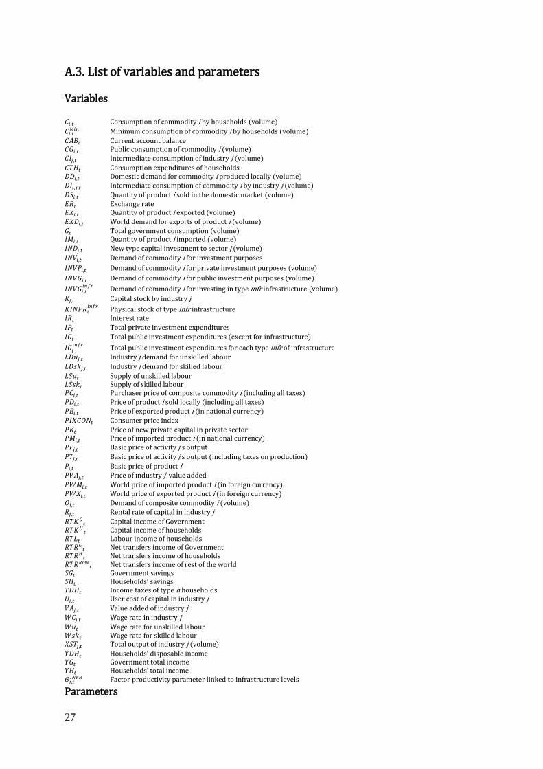
A.3. List of variables and parameters Variables 𝐶𝑖,𝑡 Consumption of commodity i by households (volume)
𝐶𝑖,𝑡𝑀𝑖𝑛 Minimum consumption of commodity i by households (volume)
𝐶𝐴𝐵𝑡 Current account balance 𝐶𝐺𝑖,𝑡 Public consumption of commodity i (volume) 𝐶𝐼𝑗,𝑡 Intermediate consumption of industry j (volume) 𝐶𝑇𝐻𝑡 Consumption expenditures of households 𝐷𝐷𝑖,𝑡 Domestic demand for commodity i produced locally (volume) 𝐷𝐼𝑖,𝑗,𝑡 Intermediate consumption of commodity i by industry j (volume) 𝐷𝑆𝑖,𝑡 Quantity of product i sold in the domestic market (volume) 𝐸𝑅𝑡 Exchange rate 𝐸𝑋𝑖,𝑡 Quantity of product i exported (volume) 𝐸𝑋𝐷𝑖,𝑡 World demand for exports of product i (volume) 𝐺𝑡 Total government consumption (volume) 𝐼𝑀𝑖,𝑡 Quantity of product i imported (volume) 𝐼𝑁𝐷𝑗,𝑡 New type capital investment to sector j (volume) 𝐼𝑁𝑉𝑖,𝑡 Demand of commodity i for investment purposes
𝐼𝑁𝑉𝑃𝑖,𝑡 Demand of commodity i for private investment purposes (volume)
𝐼𝑁𝑉𝐺𝑖,𝑡 Demand of commodity i for public investment purposes (volume)
𝐼𝑁𝑉𝐺𝑖,𝑡𝑖𝑛𝑓𝑟
Demand of commodity i for investing in type infr infrastructure (volume)
𝐾𝑗,𝑡 Capital stock by industry j
𝐾𝐼𝑁𝐹𝑅𝑡𝑖𝑛𝑓𝑟
Physical stock of type infr infrastructure 𝐼𝑅𝑡 Interest rate
𝐼𝑃𝑡 Total private investment expenditures
𝐼𝐺𝑡 Total public investment expenditures (except for infrastructure)
𝐼𝐺𝑡𝑖𝑛𝑓𝑟 Total public investment expenditures for each type infr of infrastructure
𝐿𝐷𝑢𝑗,𝑡 Industry j demand for unskilled labour
𝐿𝐷𝑠𝑘𝑗,𝑡 Industry j demand for skilled labour
𝐿𝑆𝑢𝑡 Supply of unskilled labour 𝐿𝑆𝑠𝑘𝑡 Supply of skilled labour 𝑃𝐶𝑖,𝑡 Purchaser price of composite commodity i (including all taxes) 𝑃𝐷𝑖,𝑡 Price of product i sold locally (including all taxes) 𝑃𝐸𝑖,𝑡 Price of exported product i (in national currency) 𝑃𝐼𝑋𝐶𝑂𝑁𝑡 Consumer price index
𝑃𝐾𝑡 Price of new private capital in private sector 𝑃𝑀𝑖,𝑡 Price of imported product i (in national currency) 𝑃𝑃𝑗,𝑡 Basic price of activity j’s output
𝑃𝑇𝑗,𝑡 Basic price of activity j’s output (including taxes on production)
𝑃𝑖,𝑡 Basic price of product i’ 𝑃𝑉𝐴𝑗,𝑡 Price of industry j’ value added
𝑃𝑊𝑀𝑖,𝑡 World price of imported product i (in foreign currency) 𝑃𝑊𝑋𝑖,𝑡 World price of exported product i (in foreign currency) 𝑄𝑖,𝑡 Demand of composite commodity i (volume) 𝑅𝑗,𝑡 Rental rate of capital in industry j 𝑅𝑇𝐾𝐺
𝑡 Capital income of Government 𝑅𝑇𝐾𝐻
𝑡 Capital income of households 𝑅𝑇𝐿𝑡 Labour income of households 𝑅𝑇𝑅𝐺
𝑡 Net transfers income of Government 𝑅𝑇𝑅𝐻
𝑡 Net transfers income of households 𝑅𝑇𝑅𝑅𝑜𝑤
𝑡 Net transfers income of rest of the world 𝑆𝐺𝑡 Government savings 𝑆𝐻𝑡 Households’ savings 𝑇𝐷𝐻𝑡 Income taxes of type h households 𝑈𝑗,𝑡 User cost of capital in industry j 𝑉𝐴𝑗,𝑡 Value added of industry j 𝑊𝐶𝑗,𝑡 Wage rate in industry j 𝑊𝑢𝑡 Wage rate for unskilled labour 𝑊𝑠𝑘𝑡 Wage rate for skilled labour 𝑋𝑆𝑇𝑗,𝑡 Total output of industry j (volume) 𝑌𝐷𝐻𝑡 Households’ disposable income 𝑌𝐺𝑡 Government total income 𝑌𝐻𝑡 Households’ total income 𝛩𝑗,𝑡
𝐼𝑁𝐹𝑅 Factor productivity parameter linked to infrastructure levels
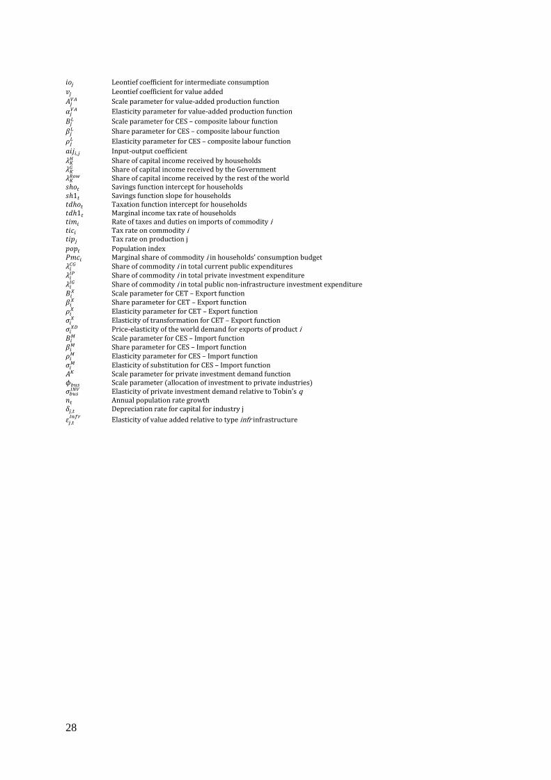
Parameters
28
𝑖𝑜𝑗 Leontief coefficient for intermediate consumption
𝑣𝑗 Leontief coefficient for value added
𝐴𝑗𝑉𝐴 Scale parameter for value-added production function
𝛼𝑗𝑉𝐴 Elasticity parameter for value-added production function
𝐵𝑗𝐿 Scale parameter for CES – composite labour function
𝛽𝑗𝐿 Share parameter for CES – composite labour function
𝜌𝑗𝐿 Elasticity parameter for CES – composite labour function
𝑎𝑖𝑗𝑖,𝑗 Input-output coefficient
𝜆𝐾𝐻 Share of capital income received by households
𝜆𝐾𝐺 Share of capital income received by the Government
𝜆𝐾𝑅𝑜𝑤 Share of capital income received by the rest of the world
𝑠ℎ𝑜𝑡 Savings function intercept for households 𝑠ℎ1𝑡 Savings function slope for households 𝑡𝑑ℎ𝑜𝑡 Taxation function intercept for households 𝑡𝑑ℎ1𝑡 Marginal income tax rate of households 𝑡𝑖𝑚𝑖 Rate of taxes and duties on imports of commodity i 𝑡𝑖𝑐𝑖 Tax rate on commodity i 𝑡𝑖𝑝𝑗 Tax rate on production j 𝑝𝑜𝑝𝑡 Population index 𝑃𝑚𝑐𝑖 Marginal share of commodity i in households’ consumption budget 𝜆𝑖
𝐶𝐺 Share of commodity i in total current public expenditures 𝜆𝑖
𝐼𝑃 Share of commodity i in total private investment expenditure 𝜆𝑖
𝐼𝐺 Share of commodity i in total public non-infrastructure investment expenditure 𝐵𝑖
𝑋 Scale parameter for CET – Export function 𝛽𝑖
𝑋 Share parameter for CET – Export function 𝜌𝑖
𝑋 Elasticity parameter for CET – Export function 𝜎𝑖
𝑋 Elasticity of transformation for CET – Export function 𝜎𝑖
𝑋𝐷 Price-elasticity of the world demand for exports of product i 𝐵𝑖
𝑀 Scale parameter for CES – Import function 𝛽𝑖
𝑀 Share parameter for CES – Import function 𝜌𝑖
𝑀 Elasticity parameter for CES – Import function 𝜎𝑖
𝑀 Elasticity of substitution for CES – Import function 𝐴𝐾 Scale parameter for private investment demand function 𝜙𝑏𝑢𝑠 Scale parameter (allocation of investment to private industries) 𝜎𝑏𝑢𝑠
𝐼𝑁𝑉 Elasticity of private investment demand relative to Tobin’s q 𝑛𝑡 Annual population rate growth 𝛿𝑗,𝑡 Depreciation rate for capital for industry j
휀𝑗,𝑡𝐼𝑛𝑓𝑟
Elasticity of value added relative to type infr infrastructure