HAL Id: hal-00110846https://hal.archives-ouvertes.fr/hal-00110846

Submitted on 2 Nov 2006

HAL is a multi-disciplinary open accessarchive for the deposit and dissemination of sci-entific research documents, whether they are pub-lished or not. The documents may come fromteaching and research institutions in France orabroad, or from public or private research centers.

L’archive ouverte pluridisciplinaire HAL, estdestinée au dépôt et à la diffusion de documentsscientifiques de niveau recherche, publiés ou non,émanant des établissements d’enseignement et derecherche français ou étrangers, des laboratoirespublics ou privés.

Centralized versus decentralized production planningG. Saharidis, Yves Dallery, F. Karaesmen

To cite this version:G. Saharidis, Yves Dallery, F. Karaesmen. Centralized versus decentralized production planning.RAIRO - Operations Research, EDP Sciences, 2006, 40, pp.113-128. <hal-00110846>

1

CENTRALIZED VERSUS DECENTRALIZED PRODUCTION PLANNING

Georges SAHARIDIS*a, Yves DALLERY*a, Fikri KARAESMEN*b

*a Ecole Centrale Paris Department of Industial Engineering (LGI), +33141131388,

saharidis,dallery@lgi.ecp.fr *b Department of Industrial Engineering, Koç University, 34450 Istanbul, Turkey

+902123381718, fkaraesmen@ku.edu.tr

Abstract

In the course of globalization, many enterprises change their strategies and are coupled in partnerships with suppliers, subcontractors and customers. This coupling forms supply chains comprising several geographically distributed production facilities. Production planning in a supply chain is a complicated and difficult task, as it has to be optimal both for the local manufacturing units and for the whole supply chain network. In this paper two analytical models are used to solve the production planning problem in supply chain involving several enterprises. Generally in practice, for competitive and/or practical reasons, frequently each enterprise prefers to optimize its production plan with little care about the other members of the supply chain. This case is presented through a simple model of decentralized optimization. The aim of this study is to analyze and compare the two types of optimization: centralized and decentralized. The initial question is: what are the profit and the optimal policy of global (centralized) optimization in contrast to local (decentralized)? We characterize this gain by comparing the optimal profits obtained in both cases. Keywords: Global-Local Optimization, Production Planning, Centralized-Decentralized models. 1. Introduction

Production planning is the process of determining a tentative plan for how much production will

occur in the next several time periods, during an interval of time called the planning horizon. Production planning also determines expected inventory levels, as well as the workforce and other resources necessary to implement the production plans. Production planning is done using an aggregate view of the production facility, the demand for products, and even of time (using monthly time periods, for example)[1]. Production planning is commonly defined as the cross-functional process of devising an aggregate production plan for groups of products over a month or quarter, based on management targets for production, sales and inventory levels. This plan should meet operating requirements for fulfilling basic business profitability and market goals and provide the overall desired framework in developing the master production schedule and in evaluating capacity and resource requirements.

In this paper, we study the production planning problem in supply chain involving several

enterprises whose final products are doors and windows made out of aluminum and compare two approaches to decision-making: decentralized versus centralized.

In section 2 we present a brief literature review and in section 3 we present our case study. In

section 4 we describe our system and the two approaches. In section 5 we give qualitative as well as numerical results from the comparison of the two approaches and in section 6 we conclude.

2

2. Literature review The supply chain is traditionally characterized by forward flow of materials and a backward flow

of information. The models for production planning of supply chain can be divided in four categories, by the modeling approach. The four categories are: (1) deterministic analytical models, in which the variables are known and specified, (2) stochastic analytical models, where at least one of the variables is unknown, and is assumed to follow a particular probability distribution, (3) simulation models, in which simulation techniques are used to evaluate the effects of various supply chain strategies on demand amplification and (4) hybrid models, in which we have an integration of analytical and simulation models. Beamon in [2] supply chain design and analysis provides a focused review of literature in multi-stage supply chain modeling and defines a research agenda for future research in this area. 2.1 Deterministic analytical models

William in [3] presents seven heuristic algorithms for scheduling production and distribution

operation. He also in [4] develops a dynamic programming algorithm for simultaneously determination of the production and distribution batch sizes at each node within a supply chain network. Morton, Kamien & Lode [5] propose, a model in which subcontracting can be explicitly considered as a production planning strategy; also possible market and no market subcontracting mechanisms and their costs are discussed. Ishii et al. [6] develop a deterministic model in order to determine the base stock levels and lead times associated with the lowest cost solution for an integrated supply chain on a finite horizon. Cohen and Lee [7] present a deterministic, mixed integer, non-linear mathematical programming model, based on economic order quantity techniques. Cohen and Moon [8] extended Cohen and Lee [7] by developing a constrained optimization model, called PILOT, to investigate the effects of various parameters on supply chain cost, and consider the additional problem of determining, which manufacturing facilities and distribution center should be open. Finally Voudouris [9] develops a mathematical model designed to improve efficiency and responsiveness in a supply chain and Camm et al [10] develop an integer programming model, based on an uncapacitated facility location formulation for Procter and Gamble Company.

2.2 Stochastic analytical models

Svoronos and Zipkin [11] consider multi-echelon, distribution-type supply chain system. In this system each facility has at most one direct predecessor, but any number of direct successors. Lee and Billington [12] develop a heuristic stochastic model for managing material flows on a site-by-site basis. Lee et al. [13] develop a stochastic, periodic-review, order-up-to inventory model to develop a procedure for process localization in the supply chain. Lee and Feitzinger [14] develop an analytical model to analyze product configuration for postponement (i.e., determining the optimal production step for production differentiation), assuming stochastic production demands. Finally Altiok and Ranjan [15] consider a generalized production/inventory system with: M (M>1) stages, one type of final product, radom processing times, setup times and intermediate buffers. The system experiences demand for finished products according to a compound Poisson process, the inventory levels for inventories are controlled according to a continuous review (R,r) inventory policy, and backorder are allowed. 2.3 Simulation models Towill [16] and Towill et al. [17] use simulation techniques to evaluate the effects of various supply chain strategies on demand amplification. The objective of the simulation model is to determine

3

which strategies are the most effective in smoothing the variations in the demand pattern. Wikner et al. [18] examine five supply chain improvement strategies, and then implement these strategies on a three-stage reference supply chain model. Their reference model includes a single factory, distribution facilities and retailers. The implementation of each of the five different strategies is carried out using simulation, the results of which are then used to determine the effects of the various strategies on minimizing demand fluctuations. 2.4 Hybrid models

Riane, Artiba and Iassinoviski [19] propose a model for a system called Hybrid Flow-shop and a

brief enumeration of the essential constraints that characterize this kind of organization. This Hybrid Flow-shop is close to our model and is a skillful combination of the ‘serial’ shop organization and the ‘parallel’ shop organization. Gnonia, et al. [20] present a case study from the automotive industry. This paper deals with lot sizing and scheduling problem (LSSP) of a multi-site manufacturing system with capacity constraints and uncertain multi-product and multi-period demand. LSSP is solved by a hybrid model resulting from the integration of a mixed-integer linear programming model and a simulation model. Yong Hae Lee and Sool Han Kim [21] propose a hybrid approach combining the analytic and simulation model for production-distribution planning in supply chain, considering capacity constraints. Byrne and Bakir [22] study a hybrid algorithm combining mathematical programming and simulation models of manufacturing system for the multi-period and multi-product production planning problem. They suggest the usefulness of a hybrid method showing the solution from the analytic model cannot de acceptable in real world. Kim and Kim [23] extend the idea of Byrne and Bakir [22] to find the capacity-feasible production plan using the analytic and the simulation model. They propose a methodology to properly modify both the left-hand and the right-hand sides of the capacity constraints in the analytic model, using the results of the simulation model. 3. Case Study

In the case study that we are planning to follow, we are interested in a conglomerate of enterprises under the name ANALKO, who’s final products are doors and windows made out of aluminum. There are several companies that belong in this conglomerate of enterprises but we are going to concentrate on the 2 major ones. The first company is in charge of purchasing the raw materials and producing a partially competed product, whereas the second company is in charge of designing the final form of the product which needs several adjustments before being released to the market. Some of those adjustments is the placement of several small parts, is the addition of paint and the placement of glass pieces. This conglomerate of enterprises doesn’t hold the 100% of the stocks for both of these two companies but they hold enough to give them the right to make decisions.

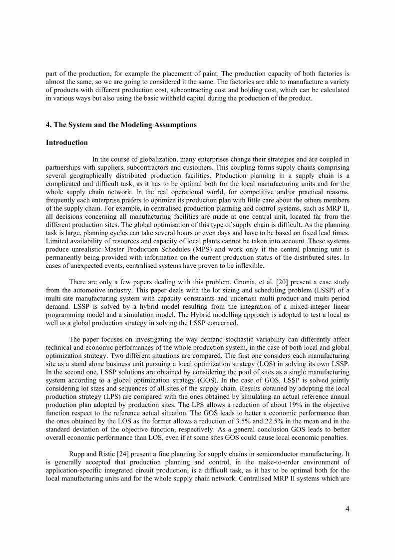
The product that we are going to talk about corresponds to a certain type of door called Type A, which is one of the basic manufactured product of this conglomerate. The demand that is presented in figure 4 is the number of doors type A sold by ANALKO in Europe in a given year multiplied by a positive number. The multiplied data were provided for reasons of confidentiality and could not reveal the true quantities. We went through the same process for the production capacities and all the certain costs that we will talk about in a later stage.

The demand has a seasonal pattern that hits its maximum value during spring and its minimum

value during winter. The companies during the time of high demand in order to cover all the extra orders, they either have to end up subcontracting, or use product that was made in previous seasons. The subcontractors have the ability to manufacture the entire product that is in demand or work on a specific

4

part of the production, for example the placement of paint. The production capacity of both factories is almost the same, so we are going to considered it the same. The factories are able to manufacture a variety of products with different production cost, subcontracting cost and holding cost, which can be calculated in various ways but also using the basic withheld capital during the production of the product. 4. The System and the Modeling Assumptions Introduction

In the course of globalization, many enterprises change their strategies and are coupled in partnerships with suppliers, subcontractors and customers. This coupling forms supply chains comprising several geographically distributed production facilities. Production planning in a supply chain is a complicated and difficult task, as it has to be optimal both for the local manufacturing units and for the whole supply chain network. In the real operational world, for competitive and/or practical reasons, frequently each enterprise prefers to optimize its production plan with little care about the others members of the supply chain. For example, in centralised production planning and control systems, such as MRP II, all decisions concerning all manufacturing facilities are made at one central unit, located far from the different production sites. The global optimisation of this type of supply chain is difficult. As the planning task is large, planning cycles can take several hours or even days and have to be based on fixed lead times. Limited availability of resources and capacity of local plants cannot be taken into account. These systems produce unrealistic Master Production Schedules (MPS) and work only if the central planning unit is permanently being provided with information on the current production status of the distributed sites. In cases of unexpected events, centralised systems have proven to be inflexible.

There are only a few papers dealing with this problem. Gnonia, et al. [20] present a case study

from the automotive industry. This paper deals with the lot sizing and scheduling problem (LSSP) of a multi-site manufacturing system with capacity constraints and uncertain multi-product and multi-period demand. LSSP is solved by a hybrid model resulting from the integration of a mixed-integer linear programming model and a simulation model. The Hybrid modelling approach is adopted to test a local as well as a global production strategy in solving the LSSP concerned.

The paper focuses on investigating the way demand stochastic variability can differently affect

technical and economic performances of the whole production system, in the case of both local and global optimization strategy. Two different situations are compared. The first one considers each manufacturing site as a stand alone business unit pursuing a local optimization strategy (LOS) in solving its own LSSP. In the second one, LSSP solutions are obtained by considering the pool of sites as a single manufacturing system according to a global optimization strategy (GOS). In the case of GOS, LSSP is solved jointly considering lot sizes and sequences of all sites of the supply chain. Results obtained by adopting the local production strategy (LPS) are compared with the ones obtained by simulating an actual reference annual production plan adopted by production sites. The LPS allows a reduction of about 19% in the objective function respect to the reference actual situation. The GOS leads to better a economic performance than the ones obtained by the LOS as the former allows a reduction of 3.5% and 22.5% in the mean and in the standard deviation of the objective function, respectively. As a general conclusion GOS leads to better overall economic performance than LOS, even if at some sites GOS could cause local economic penalties.

Rupp and Ristic [24] present a fine planning for supply chains in semiconductor manufacturing. It

is generally accepted that production planning and control, in the make-to-order environment of application-specific integrated circuit production, is a difficult task, as it has to be optimal both for the local manufacturing units and for the whole supply chain network. Centralised MRP II systems which are

5

in operation in most of today's manufacturing enterprises are not flexible enough to satisfy the demands of this highly dynamic co-operative environment. In this paper Rupp and Ristic present a distributed planning methodology for semiconductor manufacturing supply chains. The developed system is based on an approach that leaves as much responsibility and expertise for optimisation as possible to the local planning systems while a global co-ordinating entity ensures best performance and efficiency of the whole supply chain.

4.1 Our systems

We analyze the way that the system deals with the tow difference optimization strategies (Centralized versus Decentralized). We focus on investigating the way that the seasonal demand can differently affect the performances of our whole system, in the case, of both local and global optimization.

Our basic system consists of two production plants, Factory 1 (F1) and Factory 2 (F2), for which

we would like to obtain the optimal production plan, with two output stocks and two external production facilities called Subcontractor 1 and Subcontractor 2 (Subcontractor 1 gives final products to F1 and Subcontractor 2 to F2). We have a finite horizon divided into periods. The production lead time of each plant is equal to one period (between the factories or the subcontractors). In the following Figure 1 we present our system.

Our system has the ability to produce a great variety of products. We will focus in one of

these products, the one that appears to have the greatest demand in today's market. This product is a type of door made from aluminum type A. We call this product DoorTypeA (DTA). Factory 1 (F1) produces semi-finished components for F2 which produces the final product. Backorders are not allowed and all demand has to be satisfied without any delay. Each factory has a nominal production capacity and the role of the subcontractor is to provide additional external capacity if desirable. For simplicity, we assume that both initial stocks are zero and also that there is no demand for the final product during the first period. All factories have a large storage space which allows us to assume that the capacity of storing stocks is infinite. Subcontracting capacity is assumed to be infinite as well and both the production cost and the subcontracting cost are fixed during each period and proportional to the quantity of products produced or subcontracted respectively. Finally the production capacity of F1 is equal to the capacity of F2.

In the decentralized approach, we have two integrated local optimization problems from the end to

the beginning. Namely, we first optimize the production plan of F2 and then that of F1. On the other hand, in global optimization we take into account all the characteristics of the production in the F1 and F2

Factory 1

Subcontractor 1

Stock 1 Factory 2

Subcontractor 2

Stock 2

Figure 1 : The tow-stage supply chain

D2

6

simultaneously and then we optimize our system globally. The initial question is: What is to be gained by Global Optimization in contrast to Local? Below (Figure 2-3), we analyze and compare these two types of optimization and we present our results in section 5.

Two linear programming formulations are used to solve the above problems and they are presented in the appendix. Model 1 gives the solution for global optimization and model 2 for local optimization. We utilize the two models to investigate certain qualitative behavior in terms of production, inventory and subcontracting levels. Our initial question is presented by the following example:

In figure 4 we present the seasonal demand of the product DTA and the identical nominal production capacity of the two factories:

Factory 1

Subcontractor 1

Stock 1 Factory 2

Subcontractor 2

Stock 2 D2

Figure 2: Local Optimization schema

Figure 3: Global Optimization schema

Factory 1

Subcontractor 1

Stock 1 Factory 2

Subcontractor 2

Stock 2

Local Optimization

D2

Local Optimization

D1

Global Optimization

7

Demand - Production Capacity

0

20

40

60

80

100

120

140

0 5 10 15

Periods

Qua

ntiti

es

DemandeCapacité

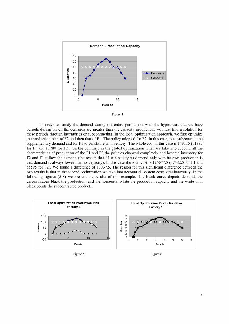
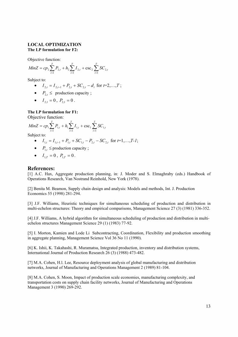
In order to satisfy the demand during the entire period and with the hypothesis that we have

periods during which the demands are greater than the capacity production, we must find a solution for these periods through inventories or subcontracting. In the local optimization approach, we first optimize the production plan of F2 and then that of F1. The policy adopted for F2, in this case, is to subcontract the supplementary demand and for F1 to constitute an inventory. The whole cost in this case is 143115 (61335 for F1 and 81780 for F2). On the contrary, in the global optimization when we take into account all the characteristics of production of the F1 and F2 the policies changed completely and became inventory for F2 and F1 follow the demand (the reason that F1 can satisfy its demand only with its own production is that demand is always lower than its capacity). In this case the total cost is 126077.5 (37482.5 for F1 and 88595 for F2). We found a difference of 17037.5. The reason for this significant difference between the two results is that in the second optimization we take into account all system costs simultaneously. In the following figures (5-8) we present the results of this example. The black curve depicts demand, the discontinuous black the production, and the horizontal white the production capacity and the white with black points the subcontracted products.

Local Optimization Production Plan Factory 2

-50

0

50

100

150

0 5 10 15

Periods

Qua

ntiti

es

Local Optimization Production PlanFactory 1

020406080

100120140

0 2 4 6 8 10 12 14

Periods

Quq

ntiti

es

Figure 4

Figure 5 Figure 6

8

Global Optimization Production PlanFactory 2

0

50

100

150

0 5 10 15

Periods

Qua

ntiti

es

Global Optimisation Production PlanFactory 1

0

50

100

150

0 5 10 15

Periods

Qua

ntiti

es

In the next section we present numerical results and the characteristics we found in our system. Details and proof can be found in [25] 5. Results 5.1 Qualitative results

We first used the two models to explore certain qualitative behavior. First of all we proved that the system’s cost of global optimization is less than or equal to that of local optimization. In terms of each one factory’s costs, the F2’s production cost in local optimization is less than or equal to that of global and F1’s is greater than or equal in local than in global. The conglomerate of enterprises that was mentioned in section 3 holds the majority of stocks of both companies. This gives them the ability to decide what kind of optimization strategy to choose. Depending on the percent of stocks they hold in each company that gives them the ability to push the production cost towards the company they hold the lowest number of stocks. For example if the percent of stocks they hold for factory 2 is larger than the percent of stocks they hold for factory 1, then even if the whole system appears to be spending, the conglomerate is still earning more money by performing local optimization of the two factories since earnings for factory 2 is maximum in the local optimization.

We were also able to show that the system’s optimal production plan is the same when the

difference between the production cost and the subcontracting cost stays constant. Also the difference between the costs of local and global optimization is constant. In reality for the subcontractor the cost of production for one unit is about the same as that of an affiliate company. The subcontractor in accordance with the contract rules wishes to receive a set amount of earnings that will not fluctuate and will be independent of the market tendencies. Thus when the market needs change, the production cost and the subcontracting cost change but the fixed amount of earnings mentioned in the contract stays the same. Using this feature we are not obliged to change the production plan when we have changed in the production cost. In addition in some cases we could be able to avoid one of two analyses. When the global optimization gives an optimal solution for F2 to subcontract the extra demand regardless of the plan of F1, the local optimization has exactly the same solution. Finally we demonstrated that when at the local optimization, the extra demand for F2 is satisfied from inventory, and then the global optimization has the same optimal plan.

Figure 7 Figure 8

9

5.2 Numerical results

In this section we present some numerical results. In Figure 9 the Relative Difference (RD) between the costs of the local and global optimizations is presented in function of inventory cost h1. For fixed h2, RD increase as function of h1 and goes up to 10% when h1 is close to h2. It becomes even greater when h1> h2 although this situation will not in general appear.

Relative Difference

-505

10152025

0 50 100Cost of Stock

Rela

tive

Diff

eren

ce

RelativeDifference

There are certain products that have about the same demand and the same production cost but the

subcontractors are demanding a different set amount of earnings for each one. So with that in mind it is very interesting to study the RD when the csc2 changes whereas the pc2 stays the same. We found that the RD increases when the subcontracting cost for F2 increases as well. We keep all cost fixed and we start with a value of csc2 equal to zero and we examine the behavior of our system in global and local optimization. We found three different intervals: • csc2<151 (extra products subcontracted ) ; • 150<csc2<550 (extra products subcontracted and stocked) ; • 551<csc2 (extra products stocked). In the next schema (Figure 10) the RD for the different cost of subcontracting is presented:

We would like to note as well that the holding cost can be calculated using the amount that has been withheld for the production of product one and which could be used in as different investment. So it is interesting to study the shape of the graph we get for RD using different values of h1.The following four schemas (figure 11-14) present the compartment of the RD when we keep the pc2 fixed and we change the h1. Based on these numerical examples, we found that we have exactly the same form. In the first space the RD is zero, in the second it increases with fluctuation and always with the peak of the graph and in the third space we have again zero.

Figure 9 : h2=50

Figure 10

Rel

ativ

e di

ffer

ence

10

Finally in the next table we present an example that shows that when the difference between the

cost of production and the cost of subcontracting stay constant, the optimal plans taken from the models are the same.

The costs h1 h2 Cp1 csc1 cp2 csc2 5 10 90 190 100 210

Production plan Inventory Production Subcontractoring

Period Factory 1 Factory 2 Factory 1 Factory 2 Factory 1 Factory 2 1 0 0 60 0 0 0 2 40 0 100 60 0 0 3 40 0 100 60 0 0 4 40 30 100 100 0 0 5 40 40 100 100 0 0 6 40 30 100 100 0 0 7 20 10 100 100 0 0 8 0 0 100 100 0 20 9 0 0 100 100 0 20

10 0 0 80 100 0 0 11 0 0 60 80 0 0 12 0 0 0 60 0 0

Figure 11 : h1=1 Figure 12 : h1=10

Figure 13 : h1=20 Figure 14 : h1=50

Rel

ativ

e di

ffer

ence

Rel

ativ

e di

ffer

ence

Rel

ativ

e di

ffer

ence

Rel

ativ

e di

ffer

ence

csc2 csc2

Table 1

11

And when we change the cp1 and csc1 we have exactly the same production plan.

Production Plan Inventory Production Subcontractoring

Period Factory 1 Factory 2 Factory 1 Factory 2 Factory 1 Factory 2 1 0 0 60 0 0 0 2 40 0 100 60 0 0 3 40 0 100 60 0 0 4 40 30 100 100 0 0 5 40 40 100 100 0 0 6 40 30 100 100 0 0 7 20 10 100 100 0 0 8 0 0 100 100 0 20 9 0 0 100 100 0 20

10 0 0 80 100 0 0 11 0 0 60 80 0 0 12 0 0 0 60 0 0

6. Conclusion:

It is known that decentralized planning results in loss of efficiency with respect to centralized

planning. It is, however, difficult to quantify the difference between the two approaches within the context of production planning. We investigated this issue in the setting of a two plant series production system. In particular, we explored a “locally optimized” production planning procedure where the downstream plant optimizes its production plan and the upstream plant follows his requests (while optimizing its costs). Then we compared this locally optimized (and decentralized) approach with global optimization where a single decision maker plans the production quantities of the supply chain in order to minimize total costs. Using a combination of analytical and numerical results, we characterized system structures which lead to small (or large) efficiency loss.

Future research could focus on development of efficient profit distribution in case of global optimization. Another interesting extension would be the analysis of an assembly system and the exploration of similarities with the model presented in this work. In this paper we have assumed that the demand as well as the processing times are deterministic. Although this assumption is true in many practical situations, it would be interesting to model systems with random processing times and random demand. This problem is subject of ongoing research.

The costs h1 h2 Cp1 csc1 cp2 csc2 5 10 100 200 110 220

Table 2

12

Appendix: Variables:

• T : Time horizon (12 months) ;

• P1,t : Production in F1 during period t ;

• I1,t : Inventory of F1 during period t ;

• SC1,t : Products subcontracted during period t in F1 ;

• P2,t : Production in F2 during period t ;

• I2,t : Inventory of F2 during period t ;

• SC2,t : Products subcontracted during period t in F2.

Costs:

• cp1 : Production cost of F1 ;

• cp2 : Production cost of F2 ;

• h1 : Inventory holding cost of F1 ;

• h2 : Inventory holding cost of F2 ;

• csc1 : Cost of subcontracted products for F1 ;

• csc2 : Cost of subcontracted products for F2.

GLOBAL OPTIMIZATION The LP formulation for F1 and F2: Objective function:

∑∑∑∑∑∑======

+++++=T

tt

T

tt

T

tt

T

tt

T

tt

T

tt SCIhPcpSCIhPcpMinZ

1,22

1,22

1,22

1,11

1,11

1,11 csccsc

Subject to: Balance equations:

• ttttt dSCPII −++= − ,2,21,2,2 for Tt ,..,2= • tttttt SCPSCPII ,2,2,1,11,1,1 −−++= − for 1,...,1 −= Tt • 01,2 =I ; • 0,1 =TI .

Production capacity: • ≤tt PP ,2,1 , production capacity for t∀ ; • 01,2 =P ; • 0,1 =TP .

13

LOCAL OPTIMIZATION The LP formulation for F2: Objective function:

∑∑∑===

++=T

tt

T

tt

T

tt SCIhPcpMinZ

1,22

1,22

1,22 csc

Subject to: • ttttt dSCPII −++= − ,2,21,2,2 for t=2,…,T ; • ≤tP ,2 production capacity ; • 01,2 =I , 01,2 =P .

The LP formulation for F1: Objective function:

∑∑∑===

++=T

tt

T

tt

T

tt SCIhPcpMinZ

1,11

1,11

1,11 csc

Subject to: • tttttt SCPSCPII ,2,2,1,11,1,1 −−++= − for t=1,…,T-1; • ≤tP ,1 production capacity ; • 0,1 =TI , 0,1 =TP .

References: [1] A.C. Hax, Aggregate production planning, in: J. Moder and S. Elmaghraby (eds.) Handbook of Operations Research, Van Nostrand Reinhold, New York (1978). [2] Benita M. Beamon, Supply chain design and analysis: Models and methods, Int. J. Production Economics 55 (1998) 281-294. [3] J.F. Williams, Heuristic techniques for simultaneous scheduling of production and distribution in multi-echelon structures: Theory and empirical comparisons, Management Science 27 (3) (1981) 336-352. [4] J.F. Williams, A hybrid algorithm for simultaneous scheduling of production and distribution in multi-echelon structures Management Science 29 (1) (1983) 77-92. [5] I. Morton, Kamien and Lode Li Subcontracting, Coordination, Flexibility and production smoothing in aggregate planning, Management Science Vol 36 No 11 (1990). [6] K. Ishii, K. Takahashi, R. Muramatsu, Integrated production, inventory and distribution systems, International Journal of Production Research 26 (3) (1988) 473-482. [7] M.A. Cohen, H.l. Lee, Resource deployment analysis of global manufacturing and distribution networks, Journal of Manufacturing and Operations Management 2 (1989) 81-104. [8] M.A. Cohen, S. Moon, Impact of production scale economies, manufacturing complexity, and transportation costs on supply chain facility networks, Journal of Manufacturing and Operations Management 3 (1990) 269-292.

14

[9] V.T. Voudouris, Mathematical programming techniques to debottleneck the supply chain of the chemical industries, Computers and Chemical Engineering 20 (1996) S1269-S1274. [10] J.D. Camm, T.E. Chorman, F.A. Dull, J.R. Evans, D.J. Sweeney, G.W. Wegryn, Blending OR/MS, judgement, and GIS: Restucturing P&G’s supply chain, Interfaces 27 (1) (1997) 128-142. [11] A. Svoronos, P.Zipkin, Evaluation of one-for-one replenishment policies for multi-echelon inventory systems, Management Science 37 (1) (1991) 68-83. [12] H.L. Lee, C. Billington, Material management in decentralized supply chain, Operations Research 41 (5) (1993) 835-847. [13] H.L. Lee, C. Billington, B. Carter, Hewlett-Packard gains control of inventory and service through design for localization, Interfaces 23 (4) (1993) 18-49. [14] H.L. Lee, E. Feitzinger, Product configuration and postponement for supply chain efficiency, Fourth Industrial Engineering Research Coference Proceeding, Institute of Industrial Engineers, 1995, pp.43-48. [15] T. Altiok, R. Ranjan, Multi-stage, pull-type production/inventory system, IIE Transaction 27 (1995) 190-200 [16] D.R. Towill, Supply chain dynamics, International Journal of Computer Integrated Manufacturing 4 (4) (1991) 197-208 [17] D.R. Towill, M.M. Naim, J. Wikner, Industrial dynamics simulation models in the design of supply chains, International Journal of Physical Distribution and Logistics Management 22 (5) (1992) 3-13 [18] J. Wikner, D.R. Towill, M.Naim, Smoothing supply chain dynamics, International Journal of Production Economics 22 (3) (1991) 231-248. [19] F. Riane, A. Artiba and S. Iassinovski, Hybrid auto-adaptable simulated annealing based heuristic, Computers & Industrial Engineering, 37, (1999) 277-280. [20] M.G. Gnonia, R. Iavagnilio, G. Mossa, G. Mummolo, A. Di Leva, Production planning of a multi-site manufacturing system by hybrid modelling: A case study from the automotive industry. Int. J. Production Economics 85 (2003) 251–262. [21] Young Hae Lee and Sook Han Kim, Production-Distribution planning in supply chain considering capacity constraints, Computers & Industrial Engineering 43 (2002) 196-190. [22] M.D. Byrne and M.A. Bakir, Production planning using a hybrid simulation-analytical approach, International Journal of Production Economics, 59 (1999) 305-311. [23] B. Kim and S Kim, Extended model of hybrid production planning approach. International Journal of Production Economics in press 2002 [24] T.M. Rupp, M. Ristic, Fine planning for supply chains in semiconductor manufacture, Journal of Materials Processing Technology 107 (2000) 390-397. [25] G. Saharidis, Y. Dallery, F. Karaesmen, Centralized versus Decentralized Production Planning in Supply Chains, Technical report, Ecole Centrale Paris, 2003.