Centralised versus Distributed Radio AccessNetworks: Wireless integration into Long Reach

Passive Optical Networks

Christian Raackatesio GmbH

Berlin, Germanyraack@atesio.de

Julio Montalvo GarciaTelefonica I+DMadrid, Spain

julio.montalvogarcia@telefonica.com

Roland Wessalyatesio GmbH

Berlin, Germanywessaely@atesio.de

Abstract—In this paper we evaluate the cost of wireless inte-gration into an architecture based on long reach passive opticalnetworks (LR-PON). We will prove that including backhaulor fronthaul signals from antenna sites into existing LR-PONstructures deployed for wired customers requires only marginaladditional resources. We will also show that scenarios withremote radio heads and centralised base band units outperformdistributed radio access networks mainly because of operationalcost savings.

I. LONG REACH PONS AND METRO CORE NODES

The FP7 project DISCUS is investigating an optimised end-to-end optical network architecture considering Long-Reach(LR) passive optical networks (PONs) and a flat optical core[1], [2]. The LR-PONs technology approach in DISCUS con-sists of a hybrid Time and Wavelength Division Multiplexing(WDM) of symmetrical 10 Gbps optical channels to commu-nicate the remote devices in a PON (ONUs) with the centraloffice equipment (OLTs). While the most advanced PONstandard is currently designed to offer up to 8 of these 10 Gbpssymmetrical channels [3], DISCUS LR-PONs are designed tosupport up to 40 of these channels [4]. Moreover, DISCUS isinvestigating and developing the technologies required in orderto support simultaneously a 100km or even 125km reach and512 split ratio in LR-PONs. With these values, DISCUS allowsa very high consolidation of PONs into a minimum numberof Points of Presence, where the access, the metro/aggregationand photonic transmission layers are comprised in the samenetwork node, namely an MC (metro-core) node.

In this respect, DISCUS revisits the classical divide betweenaccess, metro, and core networks for a new future proof end-to-end network architecture for next-generation communicationnetworks. Central to the DISCUS LR-PON is a dual-homingarchitecture, see Fig. 1. The optical signal is supposed topass a three-stage splitting hierarchy from the MC node tothe customer. The first stage splitter already located at a localexchange site, is used to provide a redundant connection to asecond MC node. In consequence, every LR-PON by-passes anLE site and is connected with two different MC nodes. Clearly,due to the quadratic scaling of connections in the full mesh ofthe optical island a small number of MC-nodes is indispensablefor this architecture to be cost-effective and scalable.

In this paper, we study the impact of wireless integrationinto an architecture based on LR-PONs. We will prove that

Fig. 1. The DISCUS LR-PON architecture: A multiple splitting hierarchybetween customer and LE and dual-homing between LE and MC. The localexchange houses the first stage 4x4 split and also acts as an amplifier node.The MC node acts as the access optical line termination as well as a corerouter with L1/2/3 switching and routing functionality.

including backhauling or fronthauling signals stemming fromantenna sites into the PON structures originally deployed forwired customers requires only marginal additional resources.We will also show that scenarios with remote radio heads andcentralised base band units outperform distributed radio accessnetworks because of operational cost savings.

II. CENTRALISED VERSUS DISTRIBUTED RADIO ACCESSNETWORKS

The centralisation of the base-band processing of radionetworks appeared as an option to traditional radio accessnetworks (RAN) because it may reduce capital and operationalcost, as well as facilitate the implementation of advanced radiofeatures such as Coordinated Multi-Point (CoMP) transmissionand reception. In centralised radio access networks (CRAN),the antenna sites are simplified with Remote Radio Heads(RRH) with no base-band processing, in opposite to thedistributed RAN (DRAN). This allows CRAN to achieve a moreeasy installation of small RRH, also allowing to reduce theoverall base-band processing resources due to the statisticalgain of centralisation. Nevertheless, it is well known that thedemand of transport resources to deliver the signals from theRRH to the Base-Band Unit (BBU), where the fronthaulingsignals are processed, increase drastically. This may reducethe opportunities for CRAN to be a cost-effective scalablesolution when considering 4G and 5G scenarios with ultra-

high speed capacity (1-10 Gbps) offered to the mobile userequipment in the radio layer. Due to the high split ratioand scalable capacity of DISCUS LR-PONs, the support ofDRAN services by the fixed fibre network seems a feasibleand cost-effective approach for fixed-wireless convergence.Nevertheless, DISCUS LR-PONs open also a new possibilityfor a cost-effective fixed-wireless convergence with CRAN,because a high number of high speed common public radiointerface (CPRI) signals can be transported into the same LR-PON using dedicated wavelengths in a Point to Point fashion,instead of requiring dedicated fibre links. We refer to Fig. 2for integrating the DRAN backhaul and CRAN fronthaul intothe LR-PON DISCUS architecture.

Fig. 2. The DISCUS LR-PON architecture with integrated antennas. a) DRANintegration, 32 sites may share the same wavelength. b) CRAN integration, eachsector requires its own wavelength in the WDM PON.

III. REFERENCE NETWORKS AND CORE NODEDISTRIBUTIONS

In order to provide realistic studies of wireless integrationinto LR-PONs including fibre routing and concrete positioningof antenna sites and local exchanges we use reference networksreflecting nation-wide fibre topologies. This approach allows toproperly incorporate the influence of topological connectivity(for resilience issues) and technological restrictions such asmaximal distances. For this study we developed referencenetworks for the UK, for Italy, and for Spain using datafrom BRITHISH TELECOM, TELECOM ITALIA, and TELEFON-ICA. The provided data sets for the UK and Italy includedanonymized (shifted) coordinates of local exchanges (centraloffices) together with the number of connected customers. ForSpain, we used detailed population statistics and high-levelcharacteristics of the local exchange distribution in Spain toestimate their positions and customer assignment.

Already in [5] and [6] we showed how to combine this op-erator specific information with public available data, namelywith data from open street maps [7], in order to come up withrealistic fibre topologies. Such geo-referenced data from streetnetworks is a reasonable choice in this case as laying fibresis typically done along streets and street networks provide

(a) (b)

(c) (d)

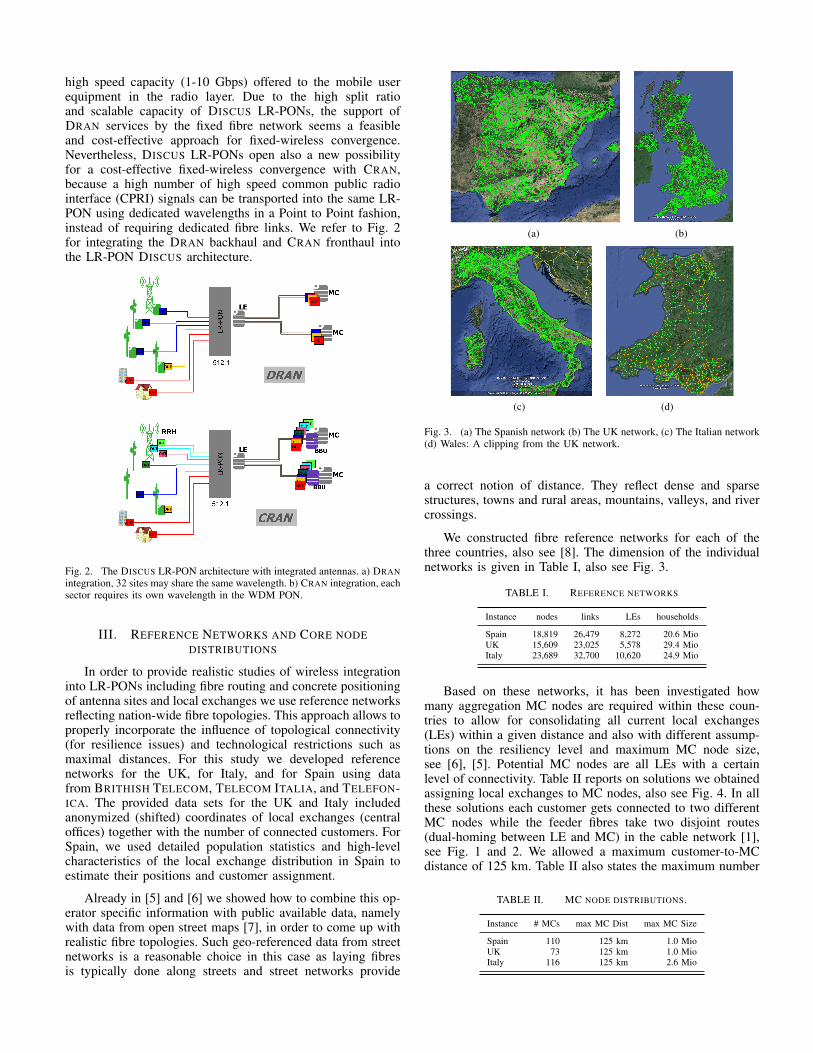
Fig. 3. (a) The Spanish network (b) The UK network, (c) The Italian network(d) Wales: A clipping from the UK network.

a correct notion of distance. They reflect dense and sparsestructures, towns and rural areas, mountains, valleys, and rivercrossings.

We constructed fibre reference networks for each of thethree countries, also see [8]. The dimension of the individualnetworks is given in Table I, also see Fig. 3.

TABLE I. REFERENCE NETWORKS

Instance nodes links LEs households

Spain 18,819 26,479 8,272 20.6 MioUK 15,609 23,025 5,578 29.4 MioItaly 23,689 32,700 10,620 24,9 Mio

Based on these networks, it has been investigated howmany aggregation MC nodes are required within these coun-tries to allow for consolidating all current local exchanges(LEs) within a given distance and also with different assump-tions on the resiliency level and maximum MC node size,see [6], [5]. Potential MC nodes are all LEs with a certainlevel of connectivity. Table II reports on solutions we obtainedassigning local exchanges to MC nodes, also see Fig. 4. In allthese solutions each customer gets connected to two differentMC nodes while the feeder fibres take two disjoint routes(dual-homing between LE and MC) in the cable network [1],see Fig. 1 and 2. We allowed a maximum customer-to-MCdistance of 125 km. Table II also states the maximum number

TABLE II. MC NODE DISTRIBUTIONS.

Instance # MCs max MC Dist max MC Size

Spain 110 125 km 1.0 MioUK 73 125 km 1.0 MioItaly 116 125 km 2.6 Mio

Fig. 4. MC node distribution in Italy: MC nodes with more than 1 Miocustomers in red, those with less than 50 K in white.

of (primary plus secondary) customers (max MC Size) at thesame MC. The Spanish (mainland) and UK solutions havebeen optimised to have at most 1 Mio customers at eachMC. In these solutions we did not respect regional boundaries(except for Northern-Ireland). For the Italian solution we didnot use a maximum customer constraint but respected regionalboundaries (20 administrative regions), that is, an LE in Venetodoes not connect to an MC in Lombardia, etc..

IV. ANTENNA SITE DISTRIBUTION

Distributing antennas to achieve full coverage within acountry is clearly a non-trivial task. Locally, it depends oncellular layout, antenna parameters such as antenna height,azimuth direction, or beamwidth, as well as regional charac-teristics such as mountains or buildings. Globally, it is furthercomplicated by the fact that the reach of the antennas and thecorresponding cell radii typically depend on the consideredgeo-type. Dense urban areas contain many base stations withsmall reach antennas (cell radii below 500m) to serve a largeamount of customers within a small area, while rural areasare served with only a few antennas and cell radii of a fewkilometres.

In order to study DRAN versus CRAN deployment andcost we start from a nation-wide distribution of antenna sitesimplementing assumptions of population density and cell radiishown in Table III. In order to determine a nation-wide geo-type distribution we use the information about connectedcustomers at the LE coordinates, see below.

Fig. 5. Tessellation with clover leaf layout: Sector and cell structure. Thesite-to-site distance is 1.5 times the site radius. This radius corresponds to thediameter of the shown hexagons, which in turn corresponds to the reach ofthe individual sector antennas.

From the mathematical perspective, given a certain cellularlayout, covering a country with cells can be seen as a tessella-tion of the plane. Hexagonal layouts as shown in Fig. 5 havebeen studied extensively, see for instance [9], [10], [11] andthe references therein. Such simplified hexagonal tessellationsand the resulting layout characteristics such as the positioningof antennas to each other and the number of sector can beused to study crucial aspects in cellular deployment such asinterference between neighboured cells.

Based on a given geo-type, our deployment of antenna sitesfollows a 3-sector hexagonal clover-leaf layout, see Fig. 5([10]). Each sector antenna spans a hexagon as shown inFig. 5 such that the antenna site sits on the edge of the threehexagons. In the following, if we speak of a (three-sector)macro cell, we refer to these three hexagons. The radius of amacro-cell is given by the reach of the sector antennas, whichresults in a site-to-site distance of 1.5 times the radius. In theresulting grid of antenna sites two rows have a distance of3√3/4 ∼ 1.3 times the macro cell radius.

Notice that we will use the terms macro cell, antenna site,and base station as synonyms throughout this paper, that is,the antenna site houses one base station and spans one macrocell (of one technology).

TABLE III. CELL MODEL BASED ON POPULATION DENSITY

Geo-Type Homes/km2 cell radius (m)

Dense Urban ≥ 4000 250Urban 2000 - 4000 500Sub-Urban 500 - 2000 1000Rural 10 - 500 2000Sparse Rural 0 - 10 10000

For deciding about the population density we considerfive geo-types: Sparse Rural, Rural, Sub-Urban, Urban, andDense Urban, which are defined by the number of householdsper square kilometre. Depending on the local geo-type wedeploy antenna sites with the radius given by Table III. Thisautomatically leads to a very dense distribution of sites in(dense) urban areas and a very sparse distribution of sites in(sparse) rural regions.

To deploy antenna sites within a given geo-type region weuse a heuristic that starts from a regular grid G as in Fig. 6(a)assuming a regular Rural tessellation with macro cells of radius2 km. The heuristic then adds or removes sites if necessary,that is, if the geo-type actually differs. In fact, we make use ofthe fact that most of the country area is actually Rural and thatthe geo-type radii are multiples of each other. We further usea description of the given country as a (typically non-convexand simple) polygon R (or several polygons if necessary). Inthis context it is important to be able to decide whether a givencoordinate point is contained in R or not, which can be donevery fast also for large polygons with many edges using thefamous crossing number algorithm [12].

The heuristic then consists of three essential steps:

1) Compute the actual geo-type geo(g) of each of the gridpoints g ∈ G by counting the number of households(connected to LEs) in a box around g. Let r(g) be themacro cell radius from Table III corresponding to geo(g).

2) Iterate the grid points g ∈ G. If r(g) < 2km, that is,if geo(g) is either Sub-Urban, Urban, or Dense Urban,

TABLE IV. MACRO CELL DEPLOYMENT: GEO-TYPE AREAS ANDRESULTING MACRO CELL DEPLOYMENT.

Country Total S.Rural Rural S.Urban Urban D.Urban

Spain Area 43.4% 53.5% 2.8% 0.2% 0.1%Macro cells 34,689 5.1% 61.8% 20.5% 6.8% 5.8%

Italy Area 11.1% 84.1% 4.4% 0.3% 0.1%Macro cells 41,276 1.0% 71.0% 17.9% 4.9% 5.2%

UK Area 23.4% 67.1% 7.7% 1.5% 0.3%Macro cells 44,309 1.2% 42.4% 24.1% 18.7% 13.7%

(a) (b)

Fig. 6. Cell deployment in the Barcelona region. The colours correspond tothe geo-types; white: Sparse Rural, yellow: Rural, light-orange: Sub-Urban,orange: Urban, red: Dense Urban; (a) Initial grid G (b) Resulting antenna sitedeployment

then a single antenna at g does not suffice to cover theneighbourhood of g. If A(Rural) is the area covered bya Rural antenna site and A(geo(g)) the area covered bya site of geo-type geo(g), then dA(Rural)/A(geo(g))egives the number of required antenna sites. We use theclover-leaf layout (Fig. 5) to distribute these sites in theconsidered area around g. For each new site we checkwhether it is contained in the countries polygon R.

3) Randomly chose one of the grid points g of type SparseRural. We place a Sparse Rural site at g. This yields acoverage area of A(SparseRural) larger than A(Rural).Remove all grid points and antenna sites in this area fromG and iterate.

Notice that the tessellation with Sparse Rural antennasites in Step 3) does not necessarily follow a regular clover-leaf structure. Further, as mentioned above, we are not givengeographical coordinates of households but of local exchanges.That is, in Step 1) we can only estimate the geo-type of a gridpoint. Given a grid point we start with a box of 3 km widthhaving the grid point in the centre to estimate the geo-type. Wethen iteratively increase the radius to 10 km. We only changethe geo-type in this iteration if the change is towards a moreurban geo-type (higher population density).

Fig. 6(b) shows an exemplary deployment using our heuris-tic in the Barcelona area. Table IV provides detailed numbersof the cell deployment for the countries Spain, Italy, and UK.It can be seen that most of the countries area is Sparse Ruraland Rural. Clearly, among the eventual macro cells there areonly few Sparse Rural because of the large radius. In contrast,the few Dense Urban regions create a significant number ofcells because of the small cell radius. The deployment dependsstrongly on the considered country. While Spain is relativelyRural there is a significant portion of (Dense) Urban cells in

the UK. Note that the number of sites in Table IV is largerbut in the same order of magnitude as those deployed todayin the considered countries.

V. PARAMETERS

In order to perform a comparison between DRAN andCRAN using LR-PONs, we focus on a future possible RANscenario. This includes the offer of a peak access of 1 Gbpsat the radio layer per cell. For DRAN, a statistical aggregationefficiency of 3.2 per antenna site is assumed, thus up to 32antenna sites could share the same 10 Gbps channel in a singleLR-PON to perform the backhaul of the IP traffic. In orderto achieve the same throughput in the CRAN approach, therequired fronthauling capacity for each sector is around 25Gbps, thus we assume a 1/3 compression ratio [13] in orderto transport the digital RoF (Radio over Fibre) signal from theRRH to the BBU using a 10 Gbps Point to Point LR-PONchannel. Due to latency restrictions required to guarantee thethroughput performance, for CRAN we also consider a limitedmaximum distance from the RRH to the BBU of 40km [14].

Translating these assumptions to side-constraints for opti-mising the LR-PONs we obtain the following

• There is no constraint on the maximum fibre distancebetween the antenna site and the metro core node forDRAN. That is, we may use the full LR-PON distanceof at most 125-km.

• There is a hard distance constraint for CRAN deployment.The base band unit can only be centralised at the MCnode if the (primary) fibre route from the antenna site tothe MC node has at most 40 km.

• At most 32 DRAN cells share the same colour in the samePON, each sites requires one port. In contrast CRAN cellsrequire 3 colours, one per sector.

• The WDM LR-PON supports up to 40 colours.

VI. WIRELESS INTEGRATION

We will study the integration of wireless backhaul andfronthaul signals starting from an existing deployment forwired customers (households). We will of course ignore PONspecific detailed aspects such as man-holes, splicing or floatingof cables, micro-ducts, etc., but concentrate on the mainstructure of the LR-PONs in terms of cabling, splitting, andport fill. We will also not consider all cost factors that arecrucial when considering PON deployments but concentrateon those resources that are effected or differ in a DRAN versusCRAN deployment. For instance, we will see that we can safelyignore duct resources as the required fibre/cable resources donot increase significantly enough neither in a DRAN nor inthe CRAN approach compared to the LR-PON deploymentbased on wired clients only. In the following, if we speakof customers, we refer to any wired client of the PON, soresidential households or business customers. This is opposedto the wireless clients, which are the antenna sites.

No coordinates for residential households are available forthe reference countries. That is, we can only estimate therequired LR-PON resources in the optical distribution network(ODN), which refers the PON segment below the LE towardsthe clients. However, we are able to determine the (lower

Fig. 7. Trees among site location in order to evaluate cell-to-LE distances.Orange dots indicate site locations (Sub-Urban and Urban). Blue dots are thelocal exchanges.

bound) of required PONs below a given local exchange asboth the number of customers at the LE as well as the numberof antenna sites is given to us. We simply assume that eachmacro site is assigned to the closest LE. Similarly, the totalnumber of required ONUs and OLTs does not depend so muchon distances but on total numbers of households, antenna sites,and resulting PONs.

In contrast, cabling and splitting in the ODN dependson the location of all PON clients. Nevertheless, with thecoordinates of antenna sites from the cellular deployment andwith some additional assumptions on average distances forhouseholds as well as assumptions on the splitter hierarchywe will at least estimate fibre distances in the ODN in orderto approximate required fibre resources. For the feeder section(between LE and MC) we have relatively accurate numbersas the cabling here only depends on the number of PONsbypassing the LE and the disjoint fibre routes towards the MCnodes, which we are given from the MC node distributionspresented in Section III.

Summarising, even without exact coordinates for buildingswe will have reasonable numbers for PON deployments in-cluding wired customers and including DRAN, CRAN cells.The numbers for fibre kilometres and splitter resources in theODN can be seen as rough estimations while the numbers forPONs, OLTs, ONUs, and required cable resources in the feedersection are very good indicators.

Given some distribution of MC nodes from Table II, adistribution of macro sites from Table IV, and an assignmentof local exchanges to a primary and secondary MC node, wecan compute the distance between an antenna site and an MCnode. The LE-to-MC fibre distance is taken from the fibre routeto the primary MC. For the antenna-to-LE distances we build aspanning tree between all sites corresponding to the same LE(the closest as mentioned above), see Fig. 7. The distance ofan antenna to the LE is defined by the unique path in that tree.Notice that we design the weights in the minimum spanningtree computation so as to (heuristically) minimise distancestowards the LE.

As mentioned above, a CRAN solution is feasible onlyif the antenna-to-MC distance is at most 40 km. However,even with this 40 km distance restriction, LR-PONs with amaximum reach of 125 km offer a good solution to cover themost populated areas with CRAN. Table V shows that for all

solutions we can reach more than 50% of the customers with acentralised radio access architecture. The share of CRAN cellsincreases with the population density. For (dense) urban areaswe achieve a coverage of typically more than 70% with valuesup to over 90% depending on the MC node density. Notice thatthe average MC node density is larger for Italy as we respectregional boundaries in the 116 node solution.

Notice that we deploy DRAN in areas where CRANis not feasible due to longer distances providing a mixedDRAN/CRAN deployment. Whenever stating a CRAN solutionwe provide the percentage CRAN coverage in brackets.

TABLE V. PERCENTAGE OF CELLS AND CUSTOMERS THAT CAN BEREACHED WITHIN 40 KM FROM THE MC FOR DIFFERENT MC-NODE

DISTRIBUTIONS. THESE SITES ARE CRAN FEASIBLE.

Reached Reached SitesCountry MCs Customers S.Rural Rural S.Urban Urban D.Urban

UK 73 65.0% 23.0% 53.0% 68.0% 70.0% 70.0%Spain 110 52.0% 26.0% 40.0% 60.0% 63.0% 64.0%Italy 116 70.0% 27.0% 50.0% 75.0% 93.0% 98.0%

a) Filling the PONs: When filling the PONs we ignoreexact positioning of both antennas and wired customers. In-stead we use the fact that each PON has two capacities: at most512 ports and at most 40 colours can be used simultaneously.To cope with topological characteristic when filling all ports ofthe same PON, we assume a filling factor of 80%, which meansthat at most 410 ports can actually be used, c. f. Fig. 8(c).There are three types of clients that use resources of the PONin a different way. Recall that each colour of the PON hasa capacity of 10 Gbps, which may be shared among the 410ports: (i) A wired customer uses one port of the PON. Atmost 410 such customer clients may use the same colour. (ii)A DRAN macro cell uses one port of the PON. At most 32such DRAN cell clients may use the same colour. (iii) A CRANmacro cell has three sectors and uses three ports of the PON.Each sector needs its own colour. Our algorithm to fill thePONS works iteratively. We simply start with the customersand fill ports, opening new PONs if necessary. We then iteratefirst the DRAN cells and then the CRAN sectors successivelyfilling the ports. We open new PONs and use new coloursif necessary. Customers always use the same colour. DRANcells use colours different from customers and CRAN sectorsuse colours different from DRAN cells and different fromcustomers. See Fig. 8 for typical PON fill statistic resultingfrom our algorithm.

b) OLTs and ONUs: Computing the number of OLTsrequired at all MC nodes to serve the PONs is simple andfollows directly from the number of used colours at the PONs.Each colour needs a serving OLT. The number of ONUs at theclient side equals the total number of used PON ports.

c) Approximating the number of splitters: To approx-imate the number of required splitters we fix the splittinghierarchy. In case of PONs for customers or DRAN cells ormixed PONs it is possible that all 410 available ports areactually used, that is, in these cases we assume a 512 splitwith a 1x8 splitter at the cabinet and a 1x16 splitter at theDP besides the 4x4 splitter at the LE, see Fig. 1. If k is thenumber of 512-PONs (customer, DRAN, or mixed PONs) thenk 4x4 amplifier splitters, 4k 1x8 cabinet splitters and 32k 1x16

(a) PONs per LE

(b) Colours per LE

(c) PON fill per LE

Fig. 8. UK solution, 73 MCs. The y-axis shows the number of LEs thatachieve the performance indicator on the x-axis. (a) Average number of PONs(b) Average number of colours (c) Average PON fill (1.0 = 512 ports; 0.8 =410 ports)

DP splitters are required. In contrast, in case of pure CRANPONs at most 40 ports can be used. We assume that the cabinetsplitter is omitted in this case. This gives a 4 · 16 = 64 split.That is, if the number of CRAN PONs is k′ then we have k′

additional 4x4 amplifier and 4k′ additional 1x16 DP splitters.

d) Approximating cabling: We will ignore the costfor ducts as we have not seen big differences in the cabledeployment for the different macro cell scenarios (only wiredcustomers, additional DRAN deployment, mixed DRAN/CRANdeployment), see below. That is, we do not expect any sig-nificant change in the duct infrastructure because of wirelessintegration if only macro cells are considered. To computecable resources in the LR-PON we distinguish drop cablesto connect clients to the PON, ODN cables for the segmentbetween first and last splitter, and feeder cables for cablingbetween LE and MC. For the latter we have precise numbersfor both the actual fibre routes and the number of fibresfollowing these routes (based on the number of PONs). Weuse a feeder cable model with cables of different sizes havingbetween 48 and 276 fibres, see Table VIII. For the Drop-section, the section between the client and the DP splitter, weuse a single-fibre cable, see Table VIII. To approximate therequired total Drop cable resources we assume Drop distancesthat depend on the geo-type. For all clients we assume an

TABLE VI. DRAN AND CRAN DEPLOYMENT AND REQUIREDSUPPLEMENT RESOURCES COMPARED TO PURE RESIDENTIAL LR-PONS

(BASE) – UK INSTANCE WITH 73 MCS, 5,578 LES, AND 44,309ANTENNA SITES, AND 29.4 MIO WIRED CUSTOMERS.

SupplementEntity Base DRAN CRAN (65%)

Backhaul Fiber km 14,078,841 0.16% 0.88%Backhaul Cable km 102,259 0.08% 0.41%D-side Fiber km 1,737,453 0.42% 1.26%Drop Fiber/Cable km 13,899,625 0.21% 0.64%

PONs 74,397 0.16% 1.14%Cabinet splitter 297,588 0.16% 0.16%DP splitter 2,380,704 0.16% 1.14%

ONUs 29,373,914 0.15% 0.34%OLTs 74,397 7.53% 114.80%

TABLE VII. DRAN AND CRAN DEPLOYMENT AND REQUIREDSUPPLEMENT RESOURCES COMPARED TO PURE WIRED CUSTOMER

LR-PONS. WE REPORT ON THE PURE MACRO-CELL DEPLOYMENT ASWELL AS ON A DEPLOYMENT WITH ADDITIONAL 8 OR 16 MICRO CELLS

PER MACRO CELL.

Country Scenario PONs Feeder ODN Splitters OLTs ONUs

UK DRAN 0.2% 0.2% 0.2% 0.2% 7.5% 0.2%CRAN(65%) 1.1% 0.9% 0.7% 1.0% 114.8% 0.3%

DRAN-8 1.3% 1.3% 3.4% 1.3% 20.9% 1.3%CRAN-8(65%) 8.7% 6.9% 3.8% 7.9% 415.3% 1.5%

DRAN-16 2.4% 2.4% 6.5% 2.4% 36.5% 2.5%CRAN-16(65%) 16.2% 12.8% 6.9% 14.7% 716.9% 2.7%

Spain DRAN 0.2% 0.2% 0.3% 0.2% 13.5% 0.2%CRAN(52%) 0.5% 0.4% 0.8% 0.4% 97.1% 0.3%

DRAN-8 1.4% 1.4% 3.4% 1.4% 25.3% 1.4%CRAN-8(52%) 6.0% 4.9% 3.9% 5.5% 335.2% 1.6%

DRAN-16 2.6% 2.6% 6.5% 2.6% 42.1% 2.7%CRAN-16(52%) 11.7% 9.5% 7.0% 10.7% 575.9% 2.9%

Italy DRAN 0.2% 0.2% 0.2% 0.2% 15.6% 0.2%CRAN(70%) 0.6% 0.6% 0.7% 0.6% 117.6% 0.4%

DRAN-8 1.3% 1.4% 3.3% 1.3% 26.0% 1.5%CRAN-8(70%) 6.5% 5.8% 3.7% 5.9% 415.3% 1.7%

DRAN-16 2.6% 2.8% 6.3% 2.6% 43.8% 2.8%CRAN-16(70%) 13.2% 11.9% 6.7% 12.0% 716.2% 3.0%

average distance of 50% of the macro cell radius correspondingto the same geo-type, that is, a distance between 125m (DenseUrban) and 5km (Sparse Rural), see Table III. For clientswithout individual geo-type we assume the same geo-type asmost of the cells at the same LE. For the ODN section andwired clients we assume an average fibre distance of 100% ofthe corresponding geo-type. However for macro cells we canobtain a more precise value since fibre distances to the localexchange can be obtained from the spanning tree mentionedabove. We follow the general assumption that the cabinetsplitter is located close to the LE. Since we assume a 1x16splitter at the DP we divide the client numbers by 16 to obtainthe number of fibres in the ODN. In the ODN we assumecables with 8 fibres on average.

Table VI shows the resources required for an LR-PONdeployment with only wired customers connected. It then alsoreports on the additional resources (in %) for a deploymentwith only DRAN cells and for a deployment where all feasiblesites are centralised following the CRAN architecture. In thiscase there are roughly 65% CRAN feasible cells, c. f. Table V.

We can clearly observe that the increase in required re-sources for wireless integration compared to existing LR-PONsconnecting all households is insignificant. Even in case of aCRAN deployment the number of PONs increases only by1.14% (0.16% for DRAN only). Notice that almost all LEshave a connected site in our solution for the UK. This meansthat if DRAN cells where integrated into PONs independentof PONs for wired customers, then the number of additionallyrequired PONs would be at least 5,449 (the number of LEs).However, we only need 120 additional PONs for DRANdeployment (0.16%). This means that most of the requiredDRAN ports could be integrated into the existing residentialPONs. The same holds for the CRAN deployment. Since thenumber of PONs does not increase significantly also all othernumbers have relatively moderate increases (splitters and fibreresources) as well. This shows that wireless convergence inLR-PONs is feasible with very low impact compared to thefixed access LR-PON deployment, both in CRAN and DRAN.

The only number that increases significantly in Table VI isthe number of OLTs. For the DRAN deployments it increasesby 8% while for CRAN deployment it increases by even 115%.Recall that residential customer PONs only occupy one colourof the WDM PON while 32 DRAN sites already require itsown colour and each sector in the CRAN deployment.

It further turns out that these observations are relativelyindependent from the actual country and MC node distribution.In Table VII we summarise the results for the differentcountries. We also tested solutions with a much larger MCnode density (not reported in the table) and we did not observeany difference in the DRAN deployment even when the numberof MCs increases drastically (we tested up to 600 MCs in theUK). However, with increasing MC node numbers the CRANcoverage increases which results in a moderate increase of thenumber of PONs and the corresponding resources for CRAN.

It can be also be observed in Table VII that the distributionof LEs and antenna sites is such that for Spain and Italy evenmore DRAN and CRAN cells can be integrated into the wiredPONs (the supplemental PON numbers are very small). In fact,the number of cells for the UK is relatively large comparedto the UK area and compared with Spain and Italy, which ismainly due to a higher population density in some areas and theresulting large number of (Dense) Urban sites, see Table IV.

We also studied a micro cell scenario where 8 or 16small cells are deployed in addition to the macro site (exceptfor Sparse Rural sites), also reported in VII (rows: DRAN-8,CRAN-8, DRAN-16, CRAN-16). The micro cells are assumedto have one sector only and are treated similar to macro cells interms of required resources. While the increase in additionallyrequired resources is still moderate in the DRAN case, itis significant for CRAN, in particular in the 16 micro cellscenario. The number of PONs increases by 11.7% to 16.2%,which results in a significant increase of the correspondingresources such as cabling in ODN and backhaul and thenumber of splitters. We note that with an increase of 10%and more of the fibre resources we can also not longer ignorethe additional cost for duct build. Clearly, the increase of cablekilometres is less than the increase in fibre kilometres, e.g. the12.8% increase in the feeder for the UK solution refers to anincrease of only 5.2% in required cables. The cables simplycontain more fibres. However this effect is not as significant

in the ODN and absent in the Drop section (1-fibre cable).We further note that if the duct build probability dependslinearly on the number of cables an a trail, then the additionalduct build in percent will be identical to the additional cableresources in percent, e.g. 5.2% in the feeder area.

VII. COST CONSIDERATIONS

So far we ignored the notion of cost. In particular, weignored the cost for the actual antenna sites. To get an idea ofthe cost difference for DRAN versus DRAN deployments weuse the techno-economical model summarised in Table VIII.Cost values are given in relation to the cost for one OLT port,which has a cost of 1.0. We assume that by centralising wecan save 50% operational and 20% capital expenditures, thatis, the cost for a CRAN RRH plus the share at the centralisedBBU is 80% of the cost of a DRAN macro site.

TABLE VIII. HARDWARE AND COST MODEL FOR LR-PON, CRAN,AND DRAN DEPLOYMENT. COST VALUES ARE GIVEN RELATIVE THE COSTOF ONE OLT PORT. CRAN SITE COST INCLUDES THE COST FOR THE RRH

AND THE BBU SHARE.

Entity DRAN CRAN

OLT port 1.00 1.00ONU port 0.04 0.03Macro site (RRH plus BBU share) 6.42 5.13Opex per macro site per year 11.43 5.72Cable kilometre ODN 8 fibres 0.38 0.38Cable kilometre Drop 1 fibre 0.07 0.07Cable kilometre feeder 48 fibres 1.05 1.05. . . . . . . . .Cable kilometre feeder 276 fibres 2.62 2.624x4 splitter and amplifier 2.39 2.391x16 splitter 0.28 0.281x8 splitter 0.18 0.18

Based on this cost model we can easily evaluate the totalcost for the LR-PON deployments in Table VI. For the UKsolution with 73 MCs we compute an up-front cost investmentfor wireline integration of 3 Mio OLTs (ignoring duct cost). InTable IX it can be seen that most of this cost is consumed byONUs and cable resources in the ODN/Drop. The increase incost for wireless integration is moderate if only macro cells areconsidered. For DRAN we pay 11,155 and for CRAN 103,801OLT units. Most of this increase is in the OLT cost, 5,602for DRAN and 85,408 for CRAN. The second largest absoluteincrease is in the total cost for cabling (Feeder plus ODN plus

TABLE IX. DRAN AND CRAN DEPLOYMENT AND REQUIREDADDITIONAL CAPITAL EXPENDITURES COMPARED TO PURE RESIDENTIAL

LR-PONS (BASE) – UK INSTANCE – BASE COST VALUES ARE GIVENW.R.T COST OF ONE OLT PORT. – WE REPORT ON THE MACRO CELL

DEPLOYMENT AND A DEPLOYMENT WITH 16 ADDITIONAL MICRO CELLSPER MACRO CELL.

SupplementEntity Base DRAN CRAN (65%) DRAN-16 CRAN-16(65%)

Feeder Cable 190,310 0.14% 0.66% 1.61% 8.91%ODN Cable 107,433 0.42% 1.26% 6.93% 7.77%Drop Cable km 968,341 0.21% 0.64% 6.41% 6.84%

Amplifier nodes 177,982 0.16% 1.14% 2.41% 16.23%Cabinet splitter 53,566 0.16% 0.16% 2.41% 2.41%DP splitter 351,551 0.16% 1.14% 2.41% 16.23%

ONUs 1,174,957 0.15% 0.30% 2.54% 2.47%OLTs 74,397 7.53% 114.80% 36.49% 716.87%

Total 3,098,536 0.36% 3.35% 4.63% 18.43%

Drop). Recall that our numbers for the Feeder are accurateestimations based on real fibre routes and a cable model withdifferent cable sizes. We do not expect a significant increase inthe cost for ducts for wireless macro cell integration. In fact,assuming a duct build probability of n · 3%, where n is thenumber of cables on a trail, we estimate a duct base cost of67,800 OLTs (in addition to the 3 Mio up-front cost) in thefeeder area, which increases by only 56 for DRAN and 275for CRAN.

In Table IX we ignore both the capital expenditures andthe operational expenditures for the antenna sites itself. Wehave 44,309 macro sites, which results in an investment of284,316 (DRAN) or 227,453 (CRAN), that is, we save 56,863with CRAN. However already the increase in the OLT costexceeds these savings. Considering the pure total investment(LR-PON cost plus site cost) a CRAN solution for the UKcosts 36,079 more than a DRAN solution. However, this is nota huge difference and since CRAN outperforms DRAN in termsof operational cost (50% savings assumed), CRAN amortisesalready in the first year (compared to DRAN, see Fig. 9(a)).If we decrease both the capital and operational savings bycentralising to only 10% per site CRAN still amortises alreadyin the second year, see Fig. 9(b).

(a)

(b)

Fig. 9. Additional capital and operational expenditures of wireless in-tegration including LR-PON resources and antenna sites. UK instance. a)capital/operational expenditures as in Table VIII b) capital/operational savingsper site by centralising only 10%.

VIII. CONCLUSION

In this paper we studied wireless integration into an accessarchitecture based on long-reach passive optical networks

and WDM. We showed that wireless/wireline convergence isfeasible as the supplement in required resources to includeantenna sites is marginal. This is in fact independent of whetherDRAN or CRAN approaches are considered. Clearly, it isadvisable to reserve capacities already when deploying PONsfor wired clients. With CRAN we observe a significant increasein the number of required OLTs, which is larger than thecapital savings at the antenna site. However since centralisingshould provide enormous savings in the operational cost, wecould show that CRAN amortises already in the first years afterthe deployment compared to DRAN. The picture changes andneeds further studying if there is a significant portion of microcells deployed and integrated into the PON. In this case evenadditional duct build might be necessary.

ACKNOWLEDGEMENT

To authors would like to thank Thomas Pfeiffer and ReneBonk for many fruitful discussions regarding wireless inte-gration. We would also like to thank Marco Schiano andAndrew Lord for providing realistic data from Telecom Italiaand British Telecom.

REFERENCES

[1] “DISCUS (FP7 Grant 318137), Deliverable 2.3, Updated referencearchitecture,” 2014.

[2] M. R. et al., “Discus: An end-to-end solution for ubiquitous broadbandoptical access,” IEEE Com. Mag., vol. 52, no. 2, 2014.

[3] “40-Gigabit-capable passive optical networks (NG-PON2): General re-quirements,” ITU-T, Series G: Transmission Systems and media, digitalsystems and media, Tech. Rep. G.989.1, 2013.

[4] “DISCUS (FP7 Grant 318137), Deliverable 4.2, System specificationsfor LR-PON implementation ,” 2014.

[5] C. Raack, N. Ascheuer, and R. Wessaly, “A nation-wide optimizationstudy on the consolidation of local exchanges using long-reach passiveoptical networks,” in Proc. ICTON, Graz, Austria, 2014, pp. 1–5.

[6] ——, “Nation-wide deployment of (long-reach) passive optical net-works: Computing the location and number of active nodes.” in Proc.ITG Fachtagung, Leipzig, Germany, 2015.

[7] OSM, “Open Street Maps, http://www.openstreetmap.org,” 2015.[8] “DISCUS (FP7 Grant 318137), Deliverable 2.6, Architectural optimiza-

tion for different geo-types,” 2014.[9] L. C. Wang, K. Chawla, and L. J. Greenstein, “Performance studies

of narrow-beam trisector cellular systems,” International Journal ofWireless Information Networks, vol. 5, no. 2, pp. 89–102, 1998.

[10] J. Itkonen, B. Tuzson, and J. Lempiainen, “Assessment of NetworkLayouts for CDMA Radio Access,” EURASIP Journal on WirelessCommunications and Networking, vol. 2008, no. 259310, 2008.

[11] M. U. Sheikh and J. Lempiainen, “A flower tessellation for simulationpurpose of cellular network with 12-sector sites,” IEEE, WirelessCommunications Letters, vol. 2, no. 3, pp. 279–282, 2013.

[12] M. Shimrat, “Algorithm 112: Position of point relative to polygon,”Communications of the ACM, vol. 5, p. 434, 1962.

[13] B. Guo, W. Cao, A. Tao, and D. Samardzija, “LTE/LTE-Asignal compression on the CPRI interface,” Bell Labs TechnicalJournal, vol. 18, no. 2, pp. 117–133, 2013. [Online]. Available:http://dx.doi.org/10.1002/bltj.21608

[14] P. Chanclou, A. Pizzinat, F. Le Clech, T.-L. Reedeker, Y. Lagadec,F. Saliou, B. Le Guyader, L. Guillo, Q. Deniel, S. Gosselin, S. Le,T. Diallo, R. Brenot, F. Lelarge, L. Marazzi, P. Parolari, M. Martinelli,S. O’Dull, S. Gebrewold, D. Hillerkuss, J. Leuthold, G. Gavioli,and P. Galli, “Optical fiber solution for mobile fronthaul to achievecloud radio access network,” in Future Network and Mobile Summit(FutureNetworkSummit), 2013, July 2013, pp. 1–11.