CENTRAL NORTH PACIFIC OCEAN - National …€ 2 ‐ 4.5 Observation models for the data 27 4.5.1 What CPUE indices should be included 27 4.5.2 Weighting of model

STOCK ASSESSMENT OF STRIPED MARLIN IN THE WESTERN AND CENTRAL NORTH PACIFIC OCEAN1

Billfish Working Group

International Scientific Committee for Tuna and Tuna‐like Species

in the North Pacific Ocean

Document prepared by:

Hui‐Hua Lee University of Hawaii, Joint Institute for Marine and Atmospheric Research 2570 Dole St., Honolulu, HI 96822

Kevin R. Piner NOAA, National Marine Fisheries Service Southwest Fisheries Science Center 8604 La Jolla Shore Dr., La Jolla, CA 92037 Robert Humphreys NOAA, National Marine Fisheries Service Pacific Islands Fisheries Science Center 99‐193 Aiea Heights Drive, Suite 417, Aiea, HI 9670 Jon Brodziak NOAA, National Marine Fisheries Service Pacific Islands Fisheries Science Center 2570 Dole St., Honolulu, HI 96822

1PIFSC Internal Report IR‐12‐035 Issued 28 August 2012. Released to public 10 January 2013.

‐ 1 ‐

TableofContents

EXECUTIVE SUMMARY .................................................................................................................................. 4

1 INTRODUCTION ................................................................................................................................... 12

2 BACKGROUND ..................................................................................................................................... 14

2.1 Biology ......................................................................................................................................... 14

2.1.1 Stock structure .................................................................................................................... 14

2.1.2 Reproduction ...................................................................................................................... 14

2.1.3 Growth ................................................................................................................................ 15

2.1.4 Movement ........................................................................................................................... 16

2.2 Fisheries ...................................................................................................................................... 17

2.3 Previous assessment ................................................................................................................... 18

3 DATA ................................................................................................................................................... 19

3.1 Spatial stratification .................................................................................................................... 19

3.2 Temporal stratification ............................................................................................................... 19

3.3 Definition of fisheries .................................................................................................................. 19

3.4 Catch and effort data .................................................................................................................. 20

3.5 Length‐frequency data ................................................................................................................ 21

4 MODEL DESCRIPTION .......................................................................................................................... 22

4.1 Stock Synthesis 3 ......................................................................................................................... 22

4.2 Biological and demographic assumptions .................................................................................. 22

4.2.1 Growth ................................................................................................................................ 22

4.2.2 Weight‐at‐length ................................................................................................................. 23

4.2.3 Sex specificity ...................................................................................................................... 23

4.2.4 Natural mortality ................................................................................................................. 23

4.2.5 Recruitment and reproduction ........................................................................................... 23

4.2.6 Maximum age ..................................................................................................................... 24

4.2.7 Initial conditions .................................................................................................................. 24

4.3 Fishery dynamics ......................................................................................................................... 25

4.3.1 Selectivity ............................................................................................................................ 25

4.3.2 Catchability ......................................................................................................................... 26

4.4 Environmental Influences ........................................................................................................... 27

‐ 2 ‐

4.5 Observation models for the data ................................................................................................ 27

4.5.1 What CPUE indices should be included .............................................................................. 27

4.5.2 Weighting of model components ....................................................................................... 28

4.6 Convergence ............................................................................................................................... 29

4.7 Sensitivity to alternative assumptions ........................................................................................ 29

4.8 Future projection ........................................................................................................................ 29

4.8.1 Basic dynamics of projections ............................................................................................. 29

4.8.1.1 Data structure for projections .......................................................................................... 30

4.8.1.2 Compilation of fleet selectivity patterns and weights at age ........................................... 31

4.8.2 Uncertainty ......................................................................................................................... 31

4.8.2.1 Initial population size-at-age ........................................................................................... 32

4.8.2.2 States of nature (future recruitment process) .................................................................. 32

4.8.2.3 Harvest scenarios ............................................................................................................ 33

5 RESULTS .............................................................................................................................................. 34

5.1 Model convergence .................................................................................................................... 34

5.2 Model fit diagnostics ................................................................................................................... 34

5.2.1 Abundance indices .............................................................................................................. 34

5.2.2 Length composition ............................................................................................................ 35

5.3 Model parameter estimates ....................................................................................................... 35

5.3.1 Selectivity ............................................................................................................................ 35

5.3.2 Catchability ......................................................................................................................... 36

5.4 Stock assessment results ............................................................................................................ 37

5.4.1 Biomass ............................................................................................................................... 37

5.4.2 Recruitment ........................................................................................................................ 37

5.4.3 Fishing mortality ................................................................................................................. 37

5.5 Biological reference points ......................................................................................................... 38

5.6 Sensitivity to alternative assumptions ........................................................................................ 38

5.6.1 CPUE data ............................................................................................................................ 38

5.6.1.1 Alternative Japan distant-water longline CPUE ............................................................. 38

5.6.1.2 Dropping CPUE for poorly fit fisheries .......................................................................... 39

5.6.2 Biological assumptions ........................................................................................................ 39

5.6.2.1 Natural mortality rate (M) ............................................................................................... 39

‐ 3 ‐

5.6.2.2 Stock-recruitment steepness (h) ...................................................................................... 39

5.6.2.3 Growth curve................................................................................................................... 40

5.6.2.4 Growth variability ........................................................................................................... 40

5.6.3 Comparison to previous assessment (2007) ....................................................................... 40

5.6.3.1 Use the previous stock assessment structure ................................................................... 40

5.6.3.2 Start catch in 1952 ........................................................................................................... 41

5.7 Future projections ....................................................................................................................... 41

6 STOCK STATUS ..................................................................................................................................... 44

6.1 Stock status ................................................................................................................................. 44

6.2 Conservation advice .................................................................................................................... 44

7 LITERATURE CITED .............................................................................................................................. 45

TABLES ......................................................................................................................................................... 52

FIGURES ....................................................................................................................................................... 65

Appendix A ................................................................................................................................................ 103

Appendix B ................................................................................................................................................ 114

‐ 4 ‐

EXECUTIVE SUMMARY Stock Identification and Distribution: The Western and Central North Pacific (WCNPO) striped marlin stock (Kajikia audax) is separated from the Eastern North Pacific stock based on newly-reported results of population genetic studies and empirical patterns in the spatial distribution of fishery catch-per-unit effort. The boundary of the Western and Central North Pacific stock is defined to be the waters of the Pacific Ocean west of 140°W and north of the equator. Catches: Catches of WCNPO striped marlin have exhibited a long-term decline since the 1970s. Catches averaged roughly 8,100 mt per year during 1970-1979 and declined by roughly 50% to an average of roughly 3,800 mt per year during 2000-2009. Reported catches in 2009 totaled about 2,560 mt, which was the lowest reported catch since 1975 (Table A). Data and Assessment: Catch data was collected from all ISC countries and from countries reporting catches to the the Western and Central Pacific Fisheries Commission (WCPFC) (Table A). The growth curve was re-estimated using newly developed ageing data and value of steepness and natural mortality were also re-estimated using available biological information. Standardized catch-per-unit effort data used to measure trends in relative abundance were provided by Japan, USA, and Chinese Taipei. The stock assessment was conducted using the Stock Synthesis assessment model. The assessment model was fit to relative abundance indices and size composition data in a likelihood-based statistical framework. Maximum likelihood estimates of model parameters, derived outputs, and their variances were used to characterize stock status and to develop stock projections. Table A. Reported catch (mt), population biomass (mt), spawning biomass (mt), relative spawning biomass (SB/SBMSY), recruitment (thousands), fishing mortality (average ages 3 and older), relative fishing mortality (F/FMSY), exploitation rate, and spawning potential ratio of Western and Central North Pacific striped marlin.

____________________________________________________________________________________________________________________

Year 2004 2005 2006 2007 2008 2009 2010 Mean1 Min1 Max1

____________________________________________________________________________________________________________________

Reported Catch 4047 3703 3706 3195 3691 2560 25602 6011 2560 10528

Population Biomass 11679 9545 10371 8430 7414 5335 6625 14141 5335 24886

Spawning Biomass 1731 2010 1992 1824 1625 1106 938 2439 909 5104

Relative Spawning Biomass 0.64 0.74 0.73 0.67 0.60 0.41 0.35 0.90 0.33 1.88

Recruitment (age 0) 116 434 125 204 133 349 326 453 116 1620

Fishing Mortality 0.58 0.56 0.62 0.58 0.86 0.84 0.75 0.79 0.53 1.46

Relative Fishing Mortality 1.22 0.95 0.92 1.01 0.95 1.41 1.37 1.30 0.86 2.38

Exploitation Rate 35% 39% 36% 38% 50% 48% 38% 44% 29% 69%

Spawning Potential Ratio 19% 19% 17% 19% 12% 13% 14% 14% 7% 21%

____________________________________________________________________________________________________________________

1 During 1975-2010

2 Assumed equal to 2009 value

‐ 5 ‐

Status of Stock: Estimates of population biomass of the WCNPO striped marlin stock exhibit a long-term decline (Figure A). Population biomass (age-1 and older) averaged roughly 18,200 mt, or 42% of unfished biomass during 1975-1979, the first 5 years of the assessment time frame, and declined to 6,625 mt, or 15% of unfished biomass in 2010. Spawning biomass (SB) is estimated to be 938 mt in 2010 (35% of , the spawning biomass to produce MSY, Figure B). Fishing mortality on the stock (average F on ages 3 and older) is currently high (Figure C) and averaged roughly F = 0.76 during 2007-2009, or 24% above . The predicted value of the spawning potential ratio (SPR, the predicted spawning output at current F as a fraction of unfished spawning output) is currently SPR2007-2009 = 14% which is 19% below the level of SPR required to produce MSY. Recruitment averaged about 328 thousand recruits during 1994-2008, which was roughly 30% below the 1975-2010 average. No target or limit reference points have been established for the WCNPO striped marlin stock under the auspices of the WCPFC. Compared to MSY-based reference points, the current (2010) spawning biomass is 65% below

and the current fishing mortality (average F for 2007-2009) exceeds by 24% (Figures D and E). Therefore, overfishing is currently occurring relative to MSY and the stock is in an overfished state.

Figure A. Trends in population biomass and reported catch biomass of Western and Central North Pacific striped marlin (Kajikia audax) during 1975-2010.

‐ 6 ‐

Figure B. Trends in estimates of spawning biomass of Western and Central North Pacific striped marlin (Kajikia audax) during 1975-2010 along with 80% confidence intervals.

Figure C. Trends in estimates of fishing mortality of Western and Central North Pacific striped marlin (Kajikia audax) during 1975-2010 along with 80% confidence intervals.

‐ 7 ‐

Figure D. Kobe plot of the trends in estimates of relative fishing mortality and relative spawning biomass of Western and Central North Pacific striped marlin (Kajikia audax) during 1975-2010.

Figure E. Kobe plot of the trends in estimates of relative fishing intensity and relative spawning biomass of Western and Central North Pacific striped marlin (Kajikia audax) during 1975-2010.

‐ 8 ‐

Projections: Stock projections for landings, spawning biomass, and fishing mortality of WCNPO striped marlin during 2012 to 2017 account for uncertainty in future stock size and recruitment. Two equally-plausible states of nature for future recruitment were assumed for the projections. These were: Recent Recruitment in which the recent recruitment pattern (1994-2008) was randomly resampled; and Stock-Recruitment Curve in which the recruitment deviations from the estimated stock-recruitment curve (1975-2008) were randomly resampled. Projections were run using an age-structured simulation model and included estimation uncertainty for the initial population size at age. Eight projected harvest scenarios1 were analyzed: (1) constant fishing mortality equal to the current F (SPR=0.14), the 2007-2009 average (SPR=0.12); (2) constant fishing mortality equal to FMSY (SPR=0.178); (3) constant fishing mortality equal to the 2001-2003 average (F2001-2003 = 0.90); (4) constant fishing mortality equal to the SPR of 0.2; (5) constant fishing mortality equal to the SPR of 0.3; (6) no fishing; (7) constant annual catch (2,500 mt) equal to a 20% reduction from the 2007-2009 average annual catch of 3,150 mt; (8) constant annual catch (3,600 mt = 20% reduction from the highest catches during 2000-2003). The six fishing mortality-based scenarios assumed current fishing mortality (Fcurrent) during 2010-2011 while the two catch-based scenarios assumed a constant annual catch during 2010-2011. Projection results show percentiles of projected relative spawning biomass in 2017 (Table B) and the median female spawning stock biomass and the median catch for each of the eight harvest scenarios (Table C1 and C2).

Conservation Advice: Reducing fishing mortality would likely increase spawning stock biomass and would improve the chances of higher recruitment. If one uses the median to measure the central tendency of the distributions of projected spawning biomass (Table B), then the projection results suggest that fishing at FMSY would lead to spawning biomass increases of roughly 45% to 72% from 2012 to 2017. Fishing at a constant catch of 2,500 mt would lead to potential increases in spawning biomass of 133% to 223% by 2017. Fishing at a constant catch of 3,600 mt would lead to potential increases in spawning biomass of 48% to 120% by 2017. In comparison, fishing at the current fishing mortality rate would lead to spawning biomass increases of 14% to 29% by 2017, while fishing at the average 2001-2003 fishing mortality rate would lead to a spawning biomass decrease of 2% under recent recruitment to an increase of 6% under the stock-recruitment curve assumption by 2017. Biological Reference Points: Reference points based on maximum sustainable yield (MSY) were estimated in the Stock Synthesis assessment model. The point estimate of maximum sustainable yield (± 1 standard error) was MSY = 5378 mt ± 144. The point estimate of the spawning biomass to produce MSY (adult biomass) was = 2713 mt ± 72. The point estimate of , the fishing mortality rate to produce MSY (average fishing mortality on ages 3 and older) was = 0.61 ± 0.01 and the corresponding equilibrium value of spawning potential ratio at MSY was = 17.8% ± 0.1%. Special Comments: The WCNPO striped marlin stock is expected to be highly productive due to its rapid growth and high resilience to reductions in spawning potential. The status of the stock is highly dependent on the magnitude of recruitment, which has been below its long-term average since 2004 (Table A). In addition, taking into account the fact that the WCNPO striped

‐ 9 ‐

marlin stock is overfished, fishery catches in areas near the stock boundary should be closely monitored. Table B. Percentiles of projected relative spawning stock biomass (SB2017/SB2012) in 2017.

Harvest Scenario 5th 25th 50th 75th 95th 5th 25th 50th 75th 95th(1) F = Fcurrent 0.85 1.03 1.14 1.23 1.36 0.83 1.09 1.29 1.51 1.82

(2) F = FMSY 1.12 1.32 1.45 1.55 1.69 1.14 1.47 1.72 1.98 2.34

(3) F = F2001-2003 0.72 0.87 0.98 1.06 1.18 0.66 0.88 1.06 1.25 1.52

(4) F = F20% 1.26 1.48 1.62 1.72 1.88 1.32 1.68 1.95 2.24 2.62(5) F = F30% 1.90 2.18 2.35 2.48 2.68 2.08 2.56 2.91 3.28 3.79(6) F = 0 4.93 5.49 5.82 6.06 6.47 5.43 6.33 7.07 7.81 8.72(7) Catch = 2500 mt 1.41 1.97 2.33 2.67 3.1 1.63 2.49 3.23 4.03 5.28(8) Catch = 3600 mt 0.98 1.18 1.48 1.80 2.25 1.05 1.51 2.20 3.01 4.37

Recent Recruitment Stock-Recruitment Curve

‐ 10 ‐

Table C1. Projected values of median spawning biomass and catch under recent recruitment.

_______________________________________________________________________________________________

Year 2012 2013 2014 2015 2016 2017

_______________________________________________________________________________________________

Scenario 1 Recent Recruitment Projection (Constant F = Fcurrent, weights in mt)

Spawning Biomass 1333 1439 1495 1510 1522 1525

Catch 3974 4113 4201 4240 4246 4224

Scenario 2 Recent Recruitment Projection (Constant F = FMSY, weights in mt)


Catch 3267 3649 3868 3948 3971 3962

Scenario 3 Recent Recruitment Projection (Constant F = F2001-2003 , weights in mt)


Catch 4471 4403 4378 4402 4399 4376

Scenario 4 Recent Recruitment Projection (Constant F = F20%, weights in mt)


Catch 2955 3412 3663 3782 3818 3819

Scenario 5 Recent Recruitment Projection (Constant F = F30%, weights in mt)


Catch 2001 2559 2912 3108 3187 3220

Scenario 6 Recent Recruitment Projection (Constant F = 0 or no fishing, weights in mt)


Catch 0 0 0 0 0 0

Scenario 7 Recent Recruitment Projection (Constant Catch = 2,500 mt, weights in mt)


Catch 2500 2500 2500 2500 2500 2500

Scenario 8 Recent Recruitment Projection (Constant Catch = 3,600 mt, weights in mt)


Catch 3600 3600 3600 3600 3600 3600

_______________________________________________________________________________________________

‐ 11 ‐

Table C2. Projected values of median spawning biomass and catch under stock-recruitment curve.

________________________________________________________________________________________________________

Year 2012 2013 2014 2015 2016 2017

________________________________________________________________________________________________________

Scenario 1 Stock-Recruitment Curve Projection (Constant F = Fcurrent, weights in mt)


Catch 3884 4154 4374 4543 4652 4745

Scenario 2 Stock-Recruitment Curve Projection (Constant F = FMSY, weights in mt)


Catch 3195 3685 4066 4374 4583 4740

Scenario 3 Stock-Recruitment Curve Projection (Constant F = F2001-2003, weights in mt)


Catch 4373 4431 4520 4586 4588 4648

Scenario 4 Stock-Recruitment Curve Projection (Constant F = F20%, weights in mt)


Catch 2890 3441 3878 4232 4491 4680

Scenario 5 Stock-Recruitment Curve Projection (Constant F = F30%, weights in mt)


Catch 1957 2574 3103 3533 3881 4139

Scenario 6 Stock-Recruitment Curve Projection (Constant F = 0 or no fishing, weights in mt)


Catch 0 0 0 0 0 0

Scenario 7 Stock-Recruitment Curve Projection (Constant Catch = 2,500 mt, weights in mt)


Catch 2500 2500 2500 2500 2500 2500

Scenario 8 Stock-Recruitment Curve Projection (Constant Catch = 3,600 mt, weights in mt)


Catch 3600 3600 3600 3600 3600 3600

________________________________________________________________________________________________________

‐ 12 ‐

1 INTRODUCTION

The Billfish Working Group (BILLWG) of the International Scientific Committee for Tuna and Tuna‐like Species in the North Pacific Ocean (ISC) is tasked with conducting regular stock assessments of billfish including swordfish and marlins to estimate population parameters, summarize stock status, and develop scientific advice on conservation needs for fisheries managers. In order to assess population status, the BILLWG rely greatly on coordination and collaboration with multi‐nations and multi‐regional fisheries management organizations (RFMOs). The first international billfish assessment was conducted in 1977 at the billfish stock assessment workshop using limited biological information and fishery data; few and infrequent assessments had been conducted on billfish since then. The ISC Marlin Working Group was established in 2002 and merged into the ISC Billfish Working Group in 2007. The BILLWG currently consists of members from coastal states and fishing entities of the region (China, Japan, Korea, Mexico, Taiwan, USA) and participants from relevant RFMOs, such as the Inter‐American Tropical Tuna Commission (IATTC) and Secretariat of the Pacific Community (SPC).

The previous ISC striped marlin (Kajikia audax formerly Tetrapturus audax; Collette et al. 2006)

assessment was completed in 2007. The assessment used data through 2004 and revealed a declining stock for north Pacific striped marlin and an estimated spawning potential ratio (SPR) at 9% of maximum (unfished level) (Piner et al. 2006; 2007). SPR is often used to gauge the health of a fish stock and the usual targeted levels are 20% to 40%. Despite evidence of high fishing pressure, it was noted that there was considerable uncertainty regarding the basic biology of the stock. In particular, the stock structure, spawner‐recruit resilience (h), natural mortality (M) and the growth rate of the species in the western and central North Pacific were highlighted as important areas of uncertainty.

Since the last stock assessment, considerable work on the biology of the species has been

completed. Based on genetics analyses the stock boundaries were changed to reflect a Western and Central North Pacific Ocean (WCNPO) stock and a separate Eastern Pacific Ocean (EPO) stock. New research has improved our understanding of length at 50% maturity (Sun et al. 2011a; 2011b) along with growth for the same area (Sun et al. 2011c; 2011d). Data for the major fisheries (Japan distant‐water longliners) were recompiled in the primary fisheries by different geographical boundaries along with different time periods to account for spatial and temporal heterogeneity within the fishery. Data was updated until 2009‐2010.

This report presents the results of the current assessment of striped marlin using new information

on life history and data corresponding with the WCNPO stock inside a length‐based age structured stock assessment model. The stock assessment was conducted during December 6‐16, 2011 in Honolulu, Hawaii (BILLWG 2012a) and the stock projection was developed during April 2‐9, 2012 at Shanghai Ocean University, Shanghai, China (BILLWG 2012b). The objectives of this assessment are to (1) understand the dynamics of WCNPO striped marlin by estimating population parameters such as time series of recruitment, biomass and fishing mortality, (2) determine stock status by summarizing in terms of an MSY‐based set of limit reference points, and (3) formulate scientific advice on conservation needs for fisheries managers by constructing a decision table based on projections using both constant catch and constant fishing mortality scenarios.

The results, conclusions and conservation advice recommended by the BILLWG are subject to approval by the ISC, after which they are submitted to the Inter‐American Tropical Tuna Commission (IATTC) and the Western and Central Pacific Fisheries Commission (WCPFC) for review and management action. The relationship between the two Pacific regional fisheries management organizations and the

‐ 13 ‐

ISC differs. A Memorandum of Cooperation (MOU) between the ISC and IATTC provides a mechanism for data exchange between the two organizations and allows IATTC scientific staff to participate as members on ISC working groups. In contrast, an MOU with the WCPFC specifically provides for the Northern Committee (NC), to make requests to the ISC and its working groups for scientific information and advice on highly migratory fish stocks north of 20°N latitude in the Pacific Ocean. The assessment documented in this report was approved by the ISC at the 12th Plenary Session in Sapporo Japan, 18‐23 July 2012 (ISC 2012).

‐ 14 ‐

2 BACKGROUND 2.1 Biology 2.1.1 Stock structure

Several stock scenarios have been proposed for striped marlin in the Pacific Ocean: a single

population within the Pacific (Shomura 1980), eastern‐western Pacific stocks (Morrow 1957), northern‐southern Pacific stocks (Kamimura and Honma 1958), and multiple regional stocks (Morgan 1992; Graves and McDowell 1994; McDowell and Graves 2008; Purcell and Edmands 2011). Morphological difference between northern and southern Pacific striped marlin and analysis of longline data showing that catch rates of striped marlin near equator in the western Pacific are exceptionally low indicate the potential for separate northern and southern stocks particularly in the west (Ueyanagi and Wares 1975). Recent genetic studies (Graves and McDowell 1994; McDowell and Graves 2008; Purcell and Edmands 2011) combined with the presence of spatially distinct spawning grounds (Bromhead et al. 2004) and the results of tagging studies (Ortiz et al. 2003), which show limited dispersal, suggest the presence of at least three clearly delineated Pacific stocks (southwest Pacific containing Australia and New Zealand; north Pacific containing Japan, Taiwan, Hawaii, and Southern California; and eastern Pacific containing Mexico, Central America, and Ecuador). Despite the genetic exclusion of Southern Californian striped marlin from the rest of the eastern Pacific, tagging data indicate that striped marlin caught in Southern California move south into Baja California, Mexico, corresponding to cooling water temperatures off California (Domeier 2006). The genetic study reported in Purcell and Edmunds (2011) also indicates a possible putative stock composed of mature Hawaii fish that is genetically distinct from the North Pacific stock consisting of Japan, southern California, and immature Hawaii fish. However, other lines of evidence are also considered including tagging, ecological, and fishery information and based on this composite information a two stock hypothesis for the management of striped marlin in the North Pacific Ocean have chosen. The following management jurisdiction boundaries are defined by the two Regional Fisheries Management Organizations, WCPFC and IATTC (Figure 1):

• Western and Central North Pacific Ocean (WCNPO) stock under the auspices of the WCPFC ‐ West of 140°W and north of the equator (this assessment);

• East Pacific Ocean (EPO) stock under the auspices of the IATTC ‐ East of 145°W and north of 5°S (Hinton and Maunder 2011).

2.1.2 Reproduction

Based on larval studies of striped marlin, five spawning grounds have been identified: (1) northwest Pacific Ocean (Nishikawa et al. 1978); (2) southwest Pacific Ocean (Hanamoto 1977; Nakamura 1983); (3) northeast Pacific Ocean (González‐Armas et al. 1999; González‐Armas et al. 2006); (4) southeast Pacific Ocean (Nishikawa et al. 1978; 1985) and the central north Pacific Ocean around Hawaii (Hyde et al. 2006). Reproductive studies (Kume and Joseph 1969; Eldridge and Wares 1974; González‐Armas et al. 2006; Kopf et al. 2009; Sun et al. 2011a; 2011b; Humphreys, unpubl. ovary histology data) provide further support for these hypothetical spawning grounds.

Striped marlin females are multiple batch spawners that shed hydrated oocytes in separate

spawning events directly into the waters where external fertilization occurs. Females have asynchronous oocyte development, indeterminate fecundity, and seasonal maturation which are accompanied by increase in relative size of the gonads (Murua and Saborido‐Rey 2003; Sun et al. 2011a). Males conform to the unrestricted type of testicular development and testis only increase slightly in size (Greir 1981; Sun et al. 2011b). Some studies have found evidence for sexual dimorphism with females reaching larger

‐ 15 ‐

sizes based on length frequency analysis (Skillman and Yong 1976); however, others found little evidence of this (Ueyanagi and Wares 1975). Wang et al. (2006) reported that around Taiwan, the sex ratio skews toward females at the largest size classes although females do not attain the disparate sizes (≥ 300 cm lower jaw fork length, LJFL) of female swordfish, blue marlin, and black marlin. The diverse findings may result from sampling errors due to small sample sizes, limited size distributions collected by different fishing gear, and the location and season of sampling. In summary, sexual dimorphism of striped marlin is related to spawning season and body size. Sex ratio trends indicate that males tend to dominate during the spawning season in the northwestern Pacific (Nakamura et al. 1953) and in the eastern Pacific (Kuma and Joseph 1969), whereas mature females tend to increase with increased size of fish and dominate the population after reaching larger sizes in the northwest Pacific (Sun et al. 2011a) and southwest Pacific (Kopf et al. 2009).

Size at reproductive maturity studies indicate that for striped marlin, males mature at a smaller

size than females (Kopf et al. 2009; Sun et al. 2011a; 2011b). The estimated length‐at‐50%‐maturity is 202.6 cm LJFL for females and 188.9 cm LJFL for males in the southwestern Pacific (Kopf et al. 2009). In the northwestern Pacific, the estimated length‐at‐50%‐maturity is 178.98 cm (eye‐fork length, EFL) for females and 146.96 cm EFL for males (Sun et al. 2011a; 2011b).

Reproduction behavior and output may vary with fishing grounds. Female spawning frequency is

estimated to be 1‐2 days over 4‐41 events per spawning season in the southwestern Pacific (Kopf et al. 2009) while spawning frequency is estimated at 3.4 days in the northwestern Pacific (Sun et al. 2011a). The average batch fecundity is 3.1 million oocytes or 29.7±8 oocytes per gram of body weight in the southwestern Pacific (Kopf et al. 2009), 2.4‐6.4 million oocytes (mean of 4.4 million oocytes) or 53.6 oocytes per gram of body weight in the northwestern Pacific Ocean (Sun et al. 2011a), and 11‐29 million oocytes in the eastern Pacific Ocean (Kume and Joseph 1969; Eldridge and Wares 1974). The duration of the spawning season in the eastern North Pacific has been previously reported to occur during May‐June (Kume and Joseph 1969), June‐July (Eldridge and Wares 1974), July‐September (González‐Armas et al. 2006). In the western North Pacific, the spawning season occurs during April‐August by Sun et al. (2011a) while in the southwestern Pacific, the spawning season is during the austral summer months of November‐January (Kopf et al. 2009). In general, spawning season occurs in association with sea surface temperature (SST) above 27°C during late spring and summer, peaking around May‐June in the northern hemisphere and around November‐December in the southern hemisphere.

Although various results were compared, caution should be taken when interpreting the

literatures regarding the sampling errors and technical methodology used. Although the use of gonadal‐somatic index is adequate for determining spawning season, the use of gonad histology to estimate length at 50% maturity is the optimal technique toward improving our understanding of the reproductive cycle of striped marlin. Reproductive studies are best conducted when large sample sizes are available that encompass a broad size range of fish collected throughout the spawning season and within spawning grounds by various fishing gears.

2.1.3 Growth

Efforts to determine age and growth for billfish species are notoriously difficult to research because of their difficulty to sample, the minute size of their otoliths and typical reliance on other hardparts for age determination, the rarity of smaller size classes in fishery catches, and reliance on longline and other distant water fisheries for obtaining samples. Initial efforts to determine growth in striped marlin utilized fishery‐dependent length frequency data. Monthly or quarterly length

‐ 16 ‐

composition was analyzed to identify size modes corresponding to annual cohorts that could be tracked over time. The study by Skillman and Yong (1976) took a more quantitative approach by fitting a von Bertalanffy growth equation to the length frequency data collected from the Hawaii longline fleet during 1960‐1970. These results indicated that the harvested striped marlin samples were composed of ages 1‐5. However, due to the inherent limitations of using length‐frequency analysis, subsequent studies of billfish age and growth soon incorporated the evaluation of presumed annual growth bands in hardparts, particularly those observed in cross‐sections of dorsal spines. This remains the current technique for determining age in marlin while estimates of young ages (ages 0 to 2 years) can be provided from counts of daily growth increments within sectioned sagittal otoliths.

For the North Pacific, the first hardpart based age & growth study was conducted by Melo‐Barrera et al. (2003) based on sampling the recreational troll fishery off Cabo San Lucas, Mexico. Based on the enumeration of annual growth bands within cross‐sections of the 4th dorsal spine, a von Bertalanffy growth curve pooled over the sexes ( = 221 cm LJFL, = 0.23, = ‐1.6) was fitted over an age range of 2 to 11 year olds. Unfortunately, the Melo‐Barrera study did not have access to age 0‐1 year individuals and therefore could not corroborate the determination of the first true annulus in their dorsal spine sections using otolith‐based age estimates. A recent age & growth study that included otolith derived ages for the earliest year classes (ages 0‐1) has been recently reported for the western North Pacific off Taiwan (Sun et al. 2011c; 2011d) and indicates a faster growth rate for young fish ( = 263.44 cm LJFL, = 0.04, = ‐0.4, m = ‐2.05 for the Richards growth curve) and younger maximum observed age (6 year). The otolith‐based age estimates of small fish confirmed the extremely rapid growth (128 cm LJFL at age 0.5 year versus age 2 year in the Melo‐Barrera study) undergone by young‐of‐year fish. The Sun et al. (2011c; 2011d) study probably best estimates striped marlin age & growth as it more accurately characterizes the rapid early growth phase (using otolith daily growth increment counts) and thereby corroborates recognition of the first true annulus mark in the dorsal spine sections that are primarily used to age marlins. 2.1.4 Movement

Data that provides information on the population movement of striped marlin within the North

Pacific is based on fishery analysis of temporal and spatial catch‐per‐unit‐effort (CPUE) and length composition. These provide more inferential basis of data on wider‐scale population movement patterns. This data has shown a typical regional pattern of expansion of fish into higher latitudes during summer months but a lack of trans‐ocean movements characteristic like albacore and bluefin tuna (Squire and Suzuki 1990).

Movement data based on tagging individual fish have been accomplished through the use of

acoustic tags, various plastic tags following conventional tag‐recapture efforts, and electronic pop‐up satellite archival tags (PSATs). Studies of small scale horizontal and vertical movement of individual striped marlin were conducted in the 1980s and 1990s based on the tracking of acoustically tagged striped marlin over a period of 1‐2 days off Hawaii (Brill et al. 1993) and southern California (Holts and Bedford 1990). The tracking data from Hawaii revealed that individual movements were influenced by both ambient oceanographic currents and directed movements of the fish themselves (Brill and Lutcavage 2001). Vertical movement was predominantly confined to the mixed layer above 90 m depth. The extent of vertical movements off Hawaii were not apparently controlled by specific water temperature but rather by the relative change in water temperature with depth with a maximum temperature change of ~8°C colder from that of the ambient mixed layer temperature (Brill et al. 1993). In the southern California study, acoustically tagged fish showed a similar vertical range confined to

‐ 17 ‐

depths of about 90 m (Holts and Bedford 1990). Horizontal movements were either relatively long distance for a 1‐2 day period (16‐57 nm traversed) headed in a southerly direction from the tagging site or net movements were of a smaller scale that retained fish in the original tagging area (Holts and Bedford 1990).

Conventional tag‐recapture studies have been conducted in various regions for many years

although results are difficult to interpret due to the extremely low rate (<1%) of tag re‐captures, the restriction of tagging sites to areas in the vicinity of recreational fishing ports, and the restricted ability to interpret the intervening data between tag and recapture locations. Both conventional and PSAT tagging efforts have revealed only rare instances of trans‐Pacific and trans‐equatorial movements (Domeier 2006; Sippel et al. 2011). Regional analysis of PSAT tracks of fish tagged off southern California and the peninsula of Baja California, Mexico indicate that the California fish moved south into waters off Mexico while fish tagged off of the Baja Peninsula generally remained in the offshore vicinity of Mexico (Domeier 2006). Seasonal movements of fish tagged off California were in a southerly direction during the fall and winter while off Mexico, there was little indication that fish moved north up along the Baja Peninsula. Mexico tagged fish did move seasonally in and out of the Gulf of California and Sea of Cortez (Domeier 2006). In the southwestern Pacific, movement trajectories for PSAT tagged striped marlin revealed either directional reversals or stopping when striped marlin, moving in a northerly direction, approached the vicinity of 20‐21°S latitude. These results are consistent with the equatorial break in the distribution of striped marlin in the western and central Pacific (Sippel et al. 2011). Future PSAT tagging efforts in the northwest Pacific will be important to help determine the extent of movement in this particular region and the extent to which fish migrate east into the Hawaii region.

2.2 Fisheries

Striped marlins are a very valuable species with a long history of exploitation by Japan, USA, and Taiwan in the WCNPO (Figure 2). Most of the catch of striped marlin is harvested by longline, driftnet, and harpoon fisheries. During the 1950s and 1960s, fisheries in Japan accounted for 96% of the total harvest on average, mostly by longlining (64%) and harpooning (28%). Japan longline fleets were targeting predominantly albacore for canning and occasionally caught striped marlin at the surface waters, whereas harpoon fisheries operating in coastal waters of Japan directly targeted striped marlin were. It was the post‐World War II eastward expansion of the Japan longline fleets that resulted in the increased catches of striped marlin. By the late 1960s, longline catches of striped marlin were at their historically highest level. As Taiwan started to harvest this species in the late 1960s, Japan modernized its fishing and freezer technologies and started to target more highly valued species.

During the 1970s and 1980s, the total harvest of striped marlin was taken by longlining (54%),

drift‐netting (35%), and harpooning (7%). Longline effort became concentrated in more tropical waters and started setting their lines deeper to target adult bigeye tunas, where striped marlin were less abundant. These changes could explain the decline in striped marlin catches in the 1970s. In 1972, large‐mesh drift net fishery was introduced into the high seas of the WCNPO targeting albacore, skipjack tuna, striped marlin, and swordfish contributing about 35% of the total harvest before the United Nations moratorium on all drift‐net fishing in 1992. Since then, catch from the drift net fisheries are from coastal waters of the Exclusive Economic Zones (EEZ) of each country.

During the 1990s and 2000s, the total harvest of striped marlin was taken by longlining (64%),

drift‐netting (25%), and harpooning (2%). Since the early 1990s, catches have exhibited a long‐term decline from roughly 6,000 mt per year during 1990‐1999 to 4,200 mt per year during 2000‐2004 and

‐ 18 ‐

3,500 mt per year during 2005‐2008. Reported catches in 2009 totaled about 2,560 mt, which was the lowest reported catch since 1952. This decline was due to the decreasing fishing effort of the Japan distant water and offshore longline vessels (Kimoto and Yokawa 2010).

The spatial distribution of catch and catch‐per‐unit‐effort of striped marlin for Japan offshore and

distant‐water longliners indicated the decadal change of the operation, when the fishery expanded eastward in WCNPO during 1950s and 1960s and diminished during 1990s and 2000s (MAROWG 2006). In general, the majority of the catch was taken in subtropical areas and subtropical to temperate areas of WCNPO by Japan and Taiwan longliners, respectively (MAROWG 2006, Sun et al. 2011d), whereas catch was mostly taken in tropical areas of WCNPO by Korea and Chinese longliners (Tagami 2011). The main fishing ground of Japan coastal longliners was in the waters north of 20°N and west of 160°E. The operation for Japan high‐seas large‐mesh driftnet fishery occurred in the subtropical and temperate area in the northwest Pacific (west of the international dateline) and in the East China Sea (Yokawa 2005), whereas the operation was limited to coastal Japan around 38°N‐41°N for coastal large‐mesh driftnet fishery (Yokawa and Kimoto 2011).

2.3 Previous assessment The previous ISC striped marlin assessment was completed in 2007 using Stock Synthesis 2. There

are several main differences in the input data and structural assumptions of the current assessment compared to the base‐case from the 2007 assessment

1. Assumed one stock in north Pacific Ocean;

2. Steepness parameter (h) was assumed to be 0.7 in the 2007 base case and h=1.0 for the alternative model;

3. Natural mortality (M) was assumed to be 0.3 across age;

4. Melo‐Barrera growth curve (Melo‐Barrera et al. 2003);

5. Knife‐edged maturity was assumed with full maturity at 155 cm;

6. All fisheries were assumed to be asymptotic shape of selectivity;

7. The time period modeled was 1952‐2004;

8. Models started assuming equilibrium catch and recruitment.

For comparison to the 2007 stock assessment, two sensitivity runs were conducted. One run used the model assumptions for the above points 2‐6 from the 2007 assessment with catch, CPUE and length composition data from the current assessment was conducted. The other run used the model assumptions from the current assessment with extent catch data back to 1952. See Section 4.7 and 5.5 for details.

‐ 19 ‐

3 DATA Three types of data were used in this assessment: fishery‐specific catches, length compositions

sampled from the catches by fishery, and abundance indices derived from logbooks. These data were compiled from 1975 through 2010. Data sources (fisheries) and temporal coverage of the available datasets are summarized in Figure 2. Catch data in 2010 were considered preliminary at the time of the assessment. Details of these data and their stratification are described below.

3.1 Spatial stratification The geographic area encompassed in the assessment for the western and central north Pacific

(WCNPO) striped marlin is the waters of the Pacific Ocean west of 140°W and north of the equator (Figure 1). This represents the region of the WCNPO where all of the known catches of striped marlin has been reported since 1975. The assessment modeled a single population of striped marlin within the WCNPO region, assuming virtually instantaneous mixing of fish throughout the region. Spatial effects were partially explained by regional estimates of fishery selectivity patterns.

3.2 Temporal stratification The time period modeled in this assessment is 1975‐2010. Within this period, catch and size

composition data were compiled into seasons (January–March, April–June, July–September, and October–December). Although some fisheries have catch data time series extending back to at least 1952 and model were developed in parallel that included this early data, the data in the early period was not of the same quality. Thus, the initial year of the base model was 1975 because effort and size composition data are not consistently available prior to 1975 (Figure 2) and starting the model in the 1970s allowed for estimation of initial conditions. Early model runs indicated that model estimation of biomass dynamics prior to the mid 1970’s is influenced by the assumptions of equilibrium catch (Figure 8 in Piner et al. 2011 and Section 4.2.7).

3.3 Definition of fisheries Eighteen fisheries were defined for the assessment on the basis of country, gear type, location,

and season, which represents relatively homogeneous fishing units (Table 1). The aim was to define fisheries in which changes in selectivity and catchability between fisheries are greater than temporal changes between years and between seasons. These fisheries consisted of nine longline (USA, JPN coastal, JPN offshore and distant‐water by area, JPN other, TWN offshore, TWN distant‐water, and KOR), two driftnet (JPN high sea and coastal large‐mesh and JPN squid), one bait (JPN), one trap (JPN), one net (JPN), two harpoon (JPN), one coastal fishery (TWN offshore and coastal gillnet, coastal harpoon, coastal set net and other) and one miscellaneous longline (WCPO data including Philippines, Indonesia, China, Vanuatu, Federated States of Micronesia, and Belize). Due to spatial and temporal heterogeneity of Japan distant‐water longline fishery, three different geographical boundaries (Area 1: 0‐10°N latitude by 100°E‐140°W longitude; Area 2: 10‐50°N latitude by 100°E‐160°E longitude; Area 3: 10‐50°N latitude by 160°E‐140°W longitude) were used to characterize the fishery (BILLWG 2011b; Kanaiwa et al. 2011).

Seventeen fisheries were initially defined but further analysis indicated that a residual pattern and quarterly size observations from the Japan other fishery showed a substantial seasonal pattern of larger fish caught in the first two seasons (see Section 3.5 below on length frequency data and Figure 5). Seasonality in selectivity was modeled by splitting the Japan “other fishery” into two seasonal fisheries

‐ 20 ‐

corresponding to seasons 1‐2 and 3‐4 of the calendar year in order to reduce the influence of the misfit. Although some seasonality can be observed in other fisheries, this was important as this fishery in seasons 1 and 2 included observations of the largest fish and would likely be our assumed asymptotic fishery (see Section 4.3.1). It was noted that season 2 included both larger and smaller mode fish, but preliminary model runs showed more selectivity pattern stability if season 2 was included with season 1. All further exploration described below included the breaking of the Japan other fishery into two separate fisheries: early (seasons 1‐2) and late (seasons 3‐4) fisheries.

3.4 Catch and effort data Catch was inputted into the model seasonally (calendar year) from 1975 to 2010 for 18 individual

fisheries. Catch was recorded and reported in numbers (1,000s of fish) for Japan offshore and distant‐water longline fisheries (F1‐F3) and in weight for all other fisheries. The catch value for 2010 (for most fisheries) was assumed equal to 2009 because catch data were incomplete for 2010 at the time of the analysis.

Striped marlin catches by three major gear type (longline, driftnet, and harpoon) display seasonal

variations. Although longline fisheries operate throughout the year, a seasonal pattern in the catch distribution with the 1st season producing the largest annual catches for the JPN_DWLL1 (F1), the 1st and 2nd seasons for JPN_DWLL2 (F2), the 1st and 4th seasons for the JPN_DWLL3 (F3), the 2nd and 4th seasons for the JPN_CLL (F4), the 1st season for the TWN_LL (F13), and the 1st, 2nd, and 4th seasons for the HW_LL (F16) and KOR_LL (F18) (Table 1). Major fishing season for the high‐sea and coastal large‐mesh driftnet fisheries (F5) is the 3rd season. Harpoon fisheries (F11 and F12) targeted striped marlin in the coastal waters of Japan during 1st and 2nd seasons. Annual catches for other minor fisheries (F6‐F10, F14 and F17) were evenly partitioned into four seasons due to lack of temporal information. It is noted that costal fisheries may exhibit seasonal variations and catch should be updated based on the best available information.

Catch and effort data were compiled according to the fisheries defined in the Section 3.3 and

used to develop standardized annual indices of relative abundance. Monthly aggregated dataset were used at a spatial resolution of 5‐degree longitude by 5‐degree latitude (5x5 data) for Japan and Taiwan longline fisheries. Observer dataset with a resolution of 1‐degree latitude by 1‐degree longitude (1x1 data) were used for Hawaii‐based longline fisheries. Operational logbook data were used for Japan coastal large‐mesh driftnet fisheries. Generalized linear model (GLM) approach was used to standardize all abundance indices considering main factors including year, quarter or month, region and others depending on characteristic of the fishery. Details of the standardization procedures and sources of data used to derive these indices are described by the references cited in Table 2.

Fifteen standardized annual indices of relative abundance were developed for eight fisheries

(Table 2, Table 3, Figure 4), consisting of ten Japan longliners indices (S1‐S10), two Taiwan longliners indices (S13, S14), one Hawaii‐based longliner index (S15), and two driftnet indices (S11, S12). A season was assigned to each index based on the annual quarter in which the majority of catch is recorded. As for Japan distant‐water longline fisheries, three temporally separate indices in each area were defined as years: 1975‐1986, 1987‐1999 and 2000‐2009 to account for changes of operation, hook‐per‐basket (HPB) distribution, targeted fish and length distribution of catch. For example, the break between 1986 and 1987 was mainly due to the change of HPB targeting bigeye tuna and the break between 1999 and 2000 accounted for a shift of targeting sharks in recent years (BILLWG 2011b). Two indices (S11, S12) covering different time periods were created from Japan driftnet fishery (F5) because of the changes of

‐ 21 ‐

driftnet operation from high‐seas to coastal as well as the changes of data collection system. Also, two indices (S13, S14) covering different time periods were separated from Taiwan distant‐water longline fishery (F13) based on the availability of HPB information. Also, it is noted that zero or very low annual catches were observed before 1995 resulting in unrepresentative stock trend.

Visual inspection of all indices grouped by fishery type showed a downward trend among longline

indices in the 2000s although there is some variation in the timing and magnitude of decline. The JPNDWLL indices (S3, S6, S9) started decline in the early 2000s, but JPNCLL index (S10) started decline in the late 1990s and recent TWNLL index (S14) started decline in the mid‐2000s. A consistent trend among Japan longline indices in the early time period (S1, S4, and S7) was observed although they reached different level at the end; however, there are differences in early tend between Japan (S1, S4, S7) and Taiwan (S13) longline indices. There are conflicting tends among Japan longline indices in the middle time period (S5, S8). The coefficients of variation (CVs) of these indices estimated from GLM models were included to represent annual variability for each index. As for TWNLL indices, constant CV values of 0.4 and 0.2 are assigned to all years for S13 and S14 based on the availability of hooks‐per‐basket (proxy for depth of fishing) information for standardization and the magnitude of the fishery.

3.5 Length-frequency data

Quarterly length composition data from 1975 to 2009 were used in this assessment. Length frequency data were available for eleven fisheries (Figure 5 and Figure 6) and were compiled using 5‐cm size bins from 55 to 230 cm, where the lower boundary of each bin was used to define each bin. Each length frequency observation consisted of the actual number of striped marlin measured.

Eye fork lengths (EFL) or processed weight of striped marlin for the JPN_DWLL (F1, F2, and F3,

1975‐2009), JPN_CLL (F4, 1986‐2009), JPN_DRIFT (F5, 1980‐2009) and JPN_OTHER (F11 and F12, 1976‐2000) were measured to the nearest 1 or 5 cm or nearest 1 kg at the landing ports or onboard fishing depending on the sampling resolution for each fishery. The processed weight data were converted to EFL (Taguchi and Yokawa 2011) and all of size composition data were compiled by the National Research Institute of Far Seas Fisheries (NRIFSF), Japan.

Eye fork lengths for the TWN_LL fishery (F13, 2006‐2009) were measured to the nearest 2 cm by

crew members onboard fishing vessels and compiled by the Overseas Fisheries Development Council (OFDC) of Taiwan. Eye fork lengths for the HW_LL fishery (F16, 1994‐2010) were measured to the nearest 1 cm by observers on board fishing vessels (Courtney 2011). Length composition data from the WCPO_OTHER (F17, 1993‐2009) were measured to the nearest 1 cm and provided by the WCPFC. Length composition data for the KOR_LL fishery (F18) fishery were not used because the data were considered unrepresentative of the entire fishery with one observation.

Striped marlin grow rapidly during the first year and spawning is occurs over a 4‐6 month period

leading to high variability in the sizes of fish observed in the first year of life. In addition, it appears that the timing of peak recruitment varies both regionally and inter‐annually. Thus to reduce the contribution of variability in the observed size composition that cannot be explained by model process (e.g. single timing of recruitment), the first size bin of the observation sub model was set at 120cm. This first bin was an accumulation for fish smaller than age 1 size. Sensitivity analyses were done to assess the effects of bin definition.

‐ 22 ‐

4 MODEL DESCRIPTION 4.1 Stock Synthesis 3

A seasonal, length‐based, age‐structured, forward‐simulation population model was used to assess the status of the WCNPO striped marlin stock. The model was implemented using Stock Synthesis (SS) Version 3.20b (Methot 2011; http://nft.nefsc.noaa.gov/Stock_Synthesis_3.htm). SS is a stock assessment model that estimates the population dynamics of a stock through use of a variety of fishery dependent and fishery independent information. Although its use has historically been for ground fishes, more recently it has gained popularity for stock assessments of tunas and other migratory species in the Pacific Ocean. The structure of the model allows for Bayesian estimation processes and full integration across parameter space using the Monte Carlo Markov Chain (MCMC) algorithm.

SS3 is composed of 3 subcomponents, 1) population subcomponent that recreates an estimate of

the numbers/biomass at age of the population using estimates of natural mortality, growth, fecundity etc., 2) an observational sub‐component that consists of the observed (measured) quantities such as CPUE or proportion at length/age, and 3) a statistical sub‐component that quantifies using likelihoods the fit of the observations to the recreated population. For a complete description see (Methot 2005, 2010). This analysis uses version 3.20b.

4.2 Biological and demographic assumptions 4.2.1 Growth

The sex‐combined length at age relationship was based on otoliths from a maximum of age 6 fish (Sun et al. 2011b; 2011c). This relationship was then re‐parameterized to the von Bertalanffy growth equation used in SS (Figure 7) between eye fork length (cm) and fractional age for the WCNPO striped marlin:

)(

1212)( AAKeLLLL

where L1 and L2 are the sizes associated with ages near the youngest A1 and oldest A2 ages in the data,

L∞ is the theoretical maximum length, and K is the growth coefficient. In this assessment, L1 and L2 were

104 cm and 214 cm at age 0.3 and 15, respectively. The K and L∞ can be solved based on the length at

age and L∞ was re‐parameterized as:

)(12

1121 AAKe

LLLL

The growth parameters K, L1 and L2 were fixed in the SS model and CV on age 0.3 fish and age 15 year fish were assumed to be 0.14 and 0.08, respectively. The assumption of the larger uncertainty in the length at age of young fish was consistent with ageing study. This uncertainty in the length at age of young fish also stems from the extra variance of disparate timing of recruitment, spatial variability in growth and sexual dimorphism (although the best scientific evidence does not show sexual differences in growth). Since the growth curve used is based on observed fish size at age 6 and back calculated size at age for ages < 6, research to address on uncertainty of the size of fish after age 6 is warranted.

‐ 23 ‐

4.2.2 Weight-at-length Weight‐at‐length relationships are used to convert length to weight. The length‐weight

relationship based on the same biological samples indicated that eye fork length (EFL) and weight (W) were not statistically different between the sexes (2011b; 2011c). The sex‐combined length‐weight relationship sex‐combined is:

kg 4.68 10 cm .

where WL is weight‐at‐length L. This weight‐at‐length relationship was applied as fixed parameters in the SS (Figure 8).

4.2.3 Sex specificity This assessment assumed a single sex. Some studies indicate spatial differences in the sex ratio

with either males dominating (Nakamura et al. 1953; Kuma and Joseph 1969), or females dominating the catch (Kopf et al. 2009). However, Sun et al. (Sun et al. 2011c; 2011d) reported no differences in the observed sizes at age. Given the lack of observed sexual dimorphism and a near total lack of recording of sex in fishery data, the model assumed a single sex.

4.2.4 Natural mortality Natural mortality (M) was assumed to be age‐specific in this assessment. Age‐specific M estimates

for the WCNPO striped marlin were derived from a meta‐analysis of 9 different estimators based on empirical and life history methods to represent adult fish and a Lorenzen size‐mortality relationship (Lorenzen 1996; 2000) was used to rescale adult M to represent juvenile M (Piner and Lee 2011a; 2011b). The M estimators relied on a range of factors (e.g. maximum age, maximum size, growth rate, environmental factor) based on the same biological parameters used in this assessment. Age‐specific estimates of M were fixed in the SS model as 0.54 year‐1 for age 0, 0.47 year‐1 for age 1, 0.43 year‐1 for age 2, 0.40 year‐1 for age 3, and 0.38 year‐1 for age above 4 in this assessment (Figure 9).

4.2.5 Recruitment and reproduction

Spawning was described in Sun et al. (2011a) as taking place from late spring throughout summer (April‐August) based on gonadal examination for females. In the SS model, spawning was assumed to occur in the beginning of season 2 which is the beginning of spawning cycle. The maturity ogive is based on Sun et al. (2011a) but was refit using the parameterization used in the SS3 (Figure 10), where the size‐at‐50%‐maturity was 177 cm and slope of the logistic function was ‐0.064. Recruitment timing was assumed in the model to occur in season 3 (July‐Sept) on the basis of best model fit of early model runs (Table 4 in Piner et al. 2011).

A standard Beverton and Holt stock recruitment model was used in this assessment. The expected

annual recruitment was the function of spawning biomass with steepness (h), virgin recruitment (R0), and unfished equilibrium spawning biomass (SB0) corresponding to R0 and were assumed to follow a lognormal distribution with standard deviation (Methot 2005). Annual recruitment deviations were estimated based on the information available in the data and the central tendency that penalizes the log (recruitment) deviations for deviating from zero and assumed to sum to zero over the estimated period.

‐ 24 ‐

Log‐bias adjustment factor was used to assure that the estimated log‐normally distributed recruitments are mean unbiased.

Recruitment variability ( : the standard deviation of log‐recruitment) was initially fixed at 0.6

and iteratively rescaled in the final model to match the expected variability. The log of R0 and annual recruitment deviates were estimated by the SS base‐case model. The offset for the initial recruitment relative to virgin recruitment, R1, was assumed to be negligible and fixed at 0. The choice of estimating years with information on recruitment was based on a model run with all recruitment deviations estimated (1975‐2010). The CV of the recruitment estimates was plotted and it was assumed that data, especially length compositions (but other sources as well) provide information about individual year class strengths to inform recruitment magnitude when the CV is stabilized (Figure 11). Thus recruitment was estimated during 1975‐2008 and used the SR expectations for 2009‐2010. Early data also have some information on recruitment from early cohort before 1975 and the variability of recruitment deviances often increase as the information goes down back in time (Methot and Taylor 2011). The attempt was to select the numbers of years for which young fish can be observed for the early cohort and estimate these initial recruitment deviances in the model. Five deviations were estimated prior to the start of the model. The 5 year period was chosen because early model runs showed little information on deviates more than 5 years prior to the beginning of the data because of the fast growth before they mature around age 5. A more complex modeling process that changes the bias adjustment to account for lack of information could be used allowing for estimation of all recruitment deviations. Although this mostly affects the estimation of uncertainty, it is an area for more model development.

Steepness of the stock‐recruitment relationship (h) was defined as the fraction of recruitment

from a virgin population (R0) when the spawning stock biomass is 20% of its virgin level (SB0). Studies indicated that h is poorly estimated due to little information in the data about this quantity (Magnusson and Hilborn 2007; Conn et al. 2010, Lee et al. 2012). Lee et al. (2012) has further concluded that steepness is estimable inside the stock assessment models when the model is correctly specified for relatively low productive stocks with good contrast in spawning stock biomass. Estimating h might be imprecise and biased as WCNPO striped marlin are highly productive species. Independent estimates of steepness incorporated biological and ecological characteristic of species (Mangel et al. 2010; Brodziak et al. 2011) reported that mean h was 0.87±0.05. A fixed value at 0.87 was used in this assessment. It was noted that estimates are subject to uncertainty due to lack of information on early life history stages.

4.2.6 Maximum age

The maximum age modeled was age 15, which is treated as an accumulator for all older ages

(dynamics simplified in the accumulator). To avoid biases associated with the approximation of dynamics in the accumulator age, the maximum age was set at an age sufficient to minimize the number of fish in the accumulator bin. Given the M schedule, approximately 0.2% of unfished cohort remains by age 15.

4.2.7 Initial conditions A model must assume something about the period prior to the start of the estimation of dynamics.

Typically, two approaches are used. The first is to start the model as far back as necessary to assume the period prior to the estimation of dynamics was in an unfished or near unfished state. The other approach is to estimate (where possible) initial conditions usually assuming equilibrium catch. The

‐ 25 ‐

equilibrium catch is the catch taken from a fish stock when it is in equilibrium assuming that removals and natural mortality are balanced by stable recruitment and growth. This equilibrium catch was then used to estimate the initial fishing mortality rates in the assessment model. Since the model started in 1975, the assumption for the first approach is not applicable for the WCNPO striped marlin. Equilibrium catch was used and approximated as average catches for 1952‐1974, which is 4,700 mt and 1,800 mt taken by longline fisheries (smaller size fish) and harpoon and driftnet fisheries (larger size fish), respectively (Figure 3 and Figure 5). However, starting the model in 1975 allowed the estimation of 5 years of initial age structure. In addition, during model development the magnitude of the equilibrium catch was also estimated around 4000‐8000 mt. For the base model, the equilibrium catch (assuming asymptotic selectivity pattern for the JPN_DRIFT) was fixed at 5,000 mt (roughly MSY levels) to produce a more robust model for the subsequent sensitivity analyses. However estimates of model dynamics and reference points were nearly identical for the base model (fixed equilibrium catch) and the estimated equilibrium catch model.

4.3 Fishery dynamics Fishery dynamics describes the ways in which a given population is harvested by commercial or

recreational fisheries. Changes in fishery patterns resulted from changes in target species and fishery activity (ex. locations), effects of various types of fishing gears, and environmental changes, etc. Two processes are modeled to describe the fishery dynamics, selectivity and catchability. Selectivity is used to characterize age/length‐specific pattern for the fishery and catchability is used to scale vulnerable biomass.

4.3.1 Selectivity

Unlike the 2007 assessment, the approach for this work was to estimate selectivity patterns with as flexible a selectivity pattern parameterization as possible to minimize the influence of misfit of size composition on model dynamics (Francis 2011). In this case, flexibility can be through domed shaped and time varying patterns. Selectivity pattern is fishery‐specific and is assumed to be length‐based for the WCNPO striped marlin because it affects the size distribution of the fish taken by the gear. Selectivity is also used to model fishery availability by separating fisheries into spatial stratification with separated selectivity curves (i.e. JPN_DWLL). Age‐based selectivity is also invoked that allows age 0‐15 fully selected for JPN_DWLL1, HW_LL and the WCPO_OTHER fisheries. All other fisheries were considered to select only ages 1‐15. In this assessment, selectivity patterns were estimated for all fisheries with length composition data except for KOR_LL with one observation and the same selectivity patterns were applied to the associated CPUE indices (or surveys using SS nomenclature).

Different selectivity assumptions can have large influence on the expected length‐frequency

distribution given the relative importance of length‐frequency data in the total log‐likelihood function. It then leads to the choice of the form of the selectivity curve, functional form or non‐parametric approaches. Functional forms of logistic or double normal curves were used to this assessment. Logistic curve implies that fish less than certain range of size are not vulnerable to the fishery and gradually increase vulnerability to the fishery with increase size of fish till fish are fully vulnerable (asymptotic selectivity curve). Double normal curve comprises of the outer sides of two adjacent normal curves with separate variance parameters for the left and right hand sides and peaks joined by a horizontal line implying that fishery selects certain size range of fish (dome‐shaped selectivity curve). Although dome‐shaped selectivity curve are flexible, studies have indicated that the descending limbs of selectivity

‐ 26 ‐

curves are confounded with natural mortality, catchability, and other model parameters if all fisheries are dome‐shaped (Magnusson and Hilborn 2007; Thompson 1994).

Although the goal was to use flexible selectivity parameterization, it was assumed at least one of

the fisheries has an asymptotic selectivity pattern to eliminate estimation of “cryptic biomass” and to stabilize parameter estimation. The underlying assumption means that at least one of our observational tools samples from the entire population after a specific size. This is a strong assumption that can affect estimates of depletion and scale, thus the choice of the asymptotic fishery was evaluated with cross‐pair analyses to examine which fishery or fisheries were most consistent with the assumption of asymptotic selectivity patterns in early model runs (Piner et al. 2011). The evaluation consisted of sequentially assuming one or two fisheries to be asymptotic and all other to be domed for all combinations across different growth and other model assumptions (e.g. equilibrium catch). The results indicated that the JPN_OTHER_early (F11) and JPN_DRIFT (F5) fisheries consistently produced the best fitting model when specified as asymptotic fisheries.

All model runs describe from this period forward assumed asymptotic selectivity patterns for the

JPN_OTHER_early and JPN_DRIFT fisheries (F5, F11). Two parameters described asymptotic selectivity, the length at 50% selectivity and the difference between the length at 95% selectivity and the length at 50% selectivity, were estimated in this assessment. All other fisheries (F1, F2, F3, F4, F12, F13, F16, and F17) were assumed to be domed with six parameters described the curve. The initial and final parameters of the selectivity patterns were assigned values of ‐999, which cause SS to ignore the first and last size bins and allow SS to decay the small and large fish selectivity according to parameters of ascending width and descending width, respectively. Other four parameters described dome‐shaped selectivity were estimated by the model, which are beginning size for the plateau, width of plateau, ascending width and descending width. In keeping with the theme of flexibility of selectivity parameterization and to be consistent with the changing catchability in longline cpue (e.g. 3 time specific CPUE, see Section 3.4), three time‐periods (time varying) were implemented for selectivity in F2 and F3 (1975‐1986, 1987‐1999, 2000‐2009) to account for changes in fishing practices in catch rates. Although assumption made for the changes of fishing practices was applied to 3 areas for JPN_DWLL (F1, F2, F3), the time‐periods selectivity was not implemented in the JPN_DWLL (F1) due to limited size data resulting in poor estimates (Figure 5). The influence of misfit in F1 size composition was evaluated through sensitivity analyses.

Selectivity patterns of fisheries without length composition data were mirrored to (assume) the

selectivity patterns of fisheries with similar operations and area for which a selectivity pattern was estimated. Mirrored selectivity patterns were based on expert opinion of member of the working group as follows:

1. JPN_OLL (F6) , JPN_BAIT (F8), JPN_NET (F9), and JPN_TRAP (F10) mirrored JPN_CLL (F4); 2. JPN_SQUID (F7) mirrored JPN_DRIFT (F5); 3. TWN_OSLL (F14) and TWN_CF (F15) mirrored TWN_LL (F13); 4. KOR_LL (F18) mirrored JPN_DWLL2 (F2).

4.3.2 Catchability

Catchability (q) is estimated assuming that survey indices are proportional to vulnerable biomass with a scaling factor of q and is assumed to be constant over time for all indices.

‐ 27 ‐

4.4 Environmental Influences The base‐case model does not explicitly model an environmental series or covariates. However,

environmental impacts are indirectly included in the recreation of past dynamics, such as recruitment estimates. The role of environmental versus maternal effects is evaluated in different recruitment scenarios used for future projections (see Section 4.7).

4.5 Observation models for the data

There are three data components that contribute to the log‐likelihood function, the total catch data, CPUE indices and the length‐frequency data. The observed total catch data are assumed to be unbiased and relatively precise and was fitted with a lognormal error distribution with standard error (SE) equal to 0.05. An unacceptably poor fit to catch was defined as models that did not remove >99% of the total catch from any fishery. The small CVs were for computational convenience to avoiding having to solve the Baranov equation iteratively in the multiple fisheries assessment.

The probability distributions for the CPUE indices were assumed to be lognormal distributions with SE in log space which was assumed to be the same as the CV (typically SD/estimate) in natural space described in each CPUE paper. CV was assumed to be equal to 0.2 when missing. Series with average CV<0.2 were scaled to CV=0.2 through the addition of a constant. Series with average CV>0.2 were input as given. Missing CVs were assumed =0.2 except for the TWN_LL early (S13), which was given a larger CV in accordance with the BILLWG recommendation.

The probability distributions for the length frequency data were assumed to be multinomial error distributions with the variance determined by the effective sample size (effN). In commercial fisheries, the sample of fish of a species measured is usually not a random sample of individual fish from the entire population but a sample of clusters (trips or sets). Effective sample size is usually lower than the actual number of fish sampled since a total of fish collected from clusters contain less information about the population length distribution than fish sampled randomly from population. Approximations of the input effN were taken from an analysis of the relationship with number of trips sampled in the HW_LL fleet (Courtney unpublished) which found around 10 fish per trip. Thus for all longline fisheries (F1, F2, F3, F4, F13, F16, F17) and JPN_DRIFT (F5), input effN was assumed to be number of fish measured/10 and input effN was assumed be number of fish measured for JPN_OTHER (F11, F12). A maximum quarterly sample size was assumed to be 50.

4.5.1 What CPUE indices should be included

Choices need to be made among 15 CPUE indices before weighting scheme is applied for each data component. The key question was whether an abundance data set is representative of stock abundance (and therefore shouldn’t be in conflict with other representative series). For example, if at least one of the indices covering the same time period is contradictory information, then at least one of them is likely to be unrepresentative. The working group initially discussed which series are likely to be more representative based on expert opinion. However no consensus could be reached as all series had both good and bad aspects. Thus, an objective method was used to segregate the CPUE indices into two separate data sets based on a down‐weighting analyses and correlation analyses. Two separate data sets represent two different population trajectories.

‐ 28 ‐

In the early model runs for down weighting analyses, likelihood components for indices derived from the same fishery were treated as one component with respect to inclusion or exclusion from the base model (Piner et al. 2011) as it was deemed unlikely that a fishery is representative in one time period and not another. This analysis was performed for different structural model assumptions (e.g. growth, equilibrium catch etc.) to account for model effects and summarized across these assumptions. CPUE indices were determined to provide consistent information if down‐weighting these indices led to loss of fit in the other indices. The results indicated that the JPN_DWLL1 (S1, S2, S3), JPN_DWLL_2 (S4, S5, S6), JPN_DWLL3 (S7, S8, S9) and HW_LL (S15) were consistent and considered as initial CPUE data set used for further diagnostics. The other indices including JPN_CLL (S10) and JPN_DRIFT (S11, S12), along with TWN_LL early (S13) and late (S14), were then sequentially added into the initial data set to investigate the effect of additional CPUE indices. Model diagnostics included goodness of fit to CPUE indices and length compositions were present during the stock assessment meeting (Appendix 1 in BILLWG 2012a). The results also indicated that the addition of these CPUE indices to the initial set produced no measureable improvements to the fits in CPUE and length composition data.

Correlations analyses among time series of CPUE indices were examined. Unlike down weighting

analyses, indices derived from the same fishery were treated as separate components. For example, night indices from three areas and three time stratifications (1975‐1986, 1987‐1999, 2000‐2009) for the JPN_DWLL (Brodziak and Katahira 2011) were analyzed. Pearson correlation coefficients (ρ) were interpreted as measuring the association among pairs of CPUE series showing similar results with down‐weighting analyses. The number of moderate to strong positive correlations (ρ ≥ 0.5) among CPUE time series increased from the 1975‐1986 assessment time period to the 2000‐2009 assessment time period. During 1975‐1986, there were positive correlations among the JPN_DWLL1 (S1), JPN_DWLL2 (S4), and JPN_DWLL3 (S7) indices. These indices appeared not to be consistent with the JPN_DRIFT (S11) and TWN_LL early (S13) indices. Although each index covered different time series during 1987‐1999, there were positive correlations among the JPN_DWLL2 (S5), JPN_DRIFT (S11), and TWN_LL early (S13) indices showing increasing trends. During 2000‐2009, there were positive correlations among the JPN_DWLL1 (S3), JPN_DWLL2 (S6), and JPN_DWLL3 (S9) indices, as well as JPN_CLL (S10), TWN_LL late (S14), and HW_LL (S15) indices showing decreasing trends. There was negative correlation between JPN_DRIFT (S12) and TWN_LL (S14) indices.

Based on the correlation and down‐weighting analyses, JPN_DWLL1 (S1, S2, S3), JPN_DWLL2 (S4,

S5, S6), JPN_DWLL3 (S7, S8, S9), JPN_CLL (S10), TWN_LL late (S14) and HW_LL (S15) were fitted and contributed to the total likelihood in the base case assessment (highlights in the Table 2). Iterative re‐weighting of data (see Section 4.5.2) is used subsequently to statistically down‐weight (remove) inconsistent CPUE series. The authors note that having apriori knowledge of the “best” representative index of abundance is preferable (e.g. fishery independent survey) but given the fishery dependent series and objective method of choice was necessary.

4.5.2 Weighting of model components Data‐weighting is inversely related to dataset uncertainty given to each data component in the

negative log‐likelihood function. More uncertain dataset due to small effective sample size or imprecise estimates were given less weight. The contribution of observation error to data‐weighting is the variance in datasets attributable to random sampling of a population. Determining dataset‐weighting from variety of data source is complicated when the dataset’s uncertainty contains unknown process and model‐specification errors. However, total uncertainty in datasets could be quantified with auxiliary information and statistical theory when these datasets were fitting into a model.

‐ 29 ‐

Common practice to determine the weighting among data sets is divided into two stages (Francis

2011). Weights or variances were devised using information about the way in which the data were collected (e.g. length frequency data) or statistical analyses were conducted (e.g. GLM) before the model is run. These initial weightings were provided in the Section 4.5. The second stage involved in estimating weights or variances after the model has been run so the average weights for each fishery or index in the stage 1 were adjusted to achieve internal model consistency. The model was run again with adjusted weights. These weights were applied by either adjusting additive CVs (lognormal components) or adjusting multiplicative effective sample sizes (multinomial components). In order to avoid that relative weighting given to composition data causes a poor fit to the CPUE indices data, the weighting of length composition data was adjusted in one direction, downward, where the model indicates that the weighting should be decreased as indicated by a lower estimated effective sample size. The weighting of indices was also adjusted based on the model estimate of the variability, but both increase and decrease of variance was allowed.

4.6 Convergence

Convergence to a global minimum was examined by randomly perturbing the starting values of all parameters by 10% (via jitter) and refitting the model. Improved fit (relative to the base model) would confirm that the model had not converged to the global solution.

4.7 Sensitivity to alternative assumptions

Sensitivity analyses examine the effects of plausible alternative model assumptions or configurations relative to the base‐case model results. The sensitivity analyses presented in this assessment document (Table 4) are categorized into three themes, including (1) CPUE data, (2) biology, and (3) comparison to previous assessment. For each sensitivity run, comparisons of spawning stock

biomass and fishery intensity trajectories, fits to the data if necessary, and changes in the fitted negative log‐likelihood values were completed. The attempt is to identify major source of uncertainty in the base case assessment. The authors note that many additional sensitivity runs were conducted in the development of the base case (e.g. bin definitions, initial conditions, alternative data sets etc.) that are beyond the scope of this paper to describe.

4.8 Future projection

Stock projections were conducted to evaluate the impact of various levels of fishing intensity on future spawning stock biomass and catch. The stochastic projections were implemented to incorporate variability of terminal numbers at age in the stock assessment that were propagated forward in future possibilities and uncertainty of potential future recruitment process to reflect the incompleteness of knowledge about the state of nature and ultimately, cast the results in a probabilistic analysis.

4.8.1 Basic dynamics of projections Projections were performed using software developed specifically for use with SS results in the US

West Coast groundfish fisheries, the basic dynamics are annual and were described by Punt (2010) for version 3.12b using an age‐structured population dynamics model:

‐ 30 ‐

, , ,

, ,,

,

if 0if0if

where y is the projecting year, , is the number of fish at age a in the start of year y,

is the recruitment during year y,

is the oldest age during year y, , is the total mortality at age a during year y:

,

is the instantaneous rate of natural mortality at age a,

is the fishing mortality at fully‐selected (i.e. ∑ → 1 ) age during year y,

is the selectivity by fishery f at age a,

is the relative weighting factor by fishery f determined by the proportion of maximum

selectivity at age for each fishery in which ∑ 1.

Annual fishing mortality is either specified or determined by solving the catch equation:

∑ ,

,1 , ; ∑

where is the weight at age a caught by fishery f.

To do the projections, the following quantities from the stock assessment were required: 1. Terminal numbers at age (2010) to start projection;

2. Selectivity at age ( ) for each fishery to govern age structure of catch by fishery;

3. Weight at age ( ) for each fishery to govern the weight of catch within fishery; 4. Fecundity at age ( ) (population weight at age *proportion mature at age) to calculate

spawning biomass which is ∑ , ; 5. Assumptions of future recruitment process (see Section 4.8.2); 6. Natural mortality to govern natural deaths; 7. Maximum age ( treated as a plus group for projection.

4.8.1.1 Data structure for projections Forecasts of future stock response to fishing were conducted with simplified dynamic models as

observed data were not fit in projections. The model structure for projection was listed and compared o the base‐case stock assessment (Table 5). The stock assessment calculated expected dynamics seasonally, but projections calculated dynamics (e.g. catch, spawning biomass) annually. Within the stock assessment, the first season started January 1st (January‐March) which was consistent with how data were compiled. However, for projections the year began July 1st, which corresponded to the timing

‐ 31 ‐

of recruitment in the stock assessment model (season 3). In the stock assessment model, natural mortality (M) was modeled as age specific, with each age‐class moving to the next on January 1st and therefore subjected to the next age‐classes M. Because our projections used a birth year, age specific M was a combination of the M from July‐December and next January‐June as was consistent with the stock assessment. Spawning biomass in the stock assessment model was calculated at the beginning of a protracted spawning season (season 2). In the projections, spawning biomass was calculated for July 1st. Numbers at age used to start the projection were from season 3 (July 1st) in the stock assessment model.

4.8.1.2 Compilation of fleet selectivity patterns and weights at age The assessment model contained a total of 18 individual fisheries with 10 fisheries containing

observations of the proportion of length at age. Fisheries lacking length at age data were assumed to share a selectivity pattern with a similar fishery that was consistent with the assumptions in the stock assessment (see section 4.3.1). To simplify projections the fisheries were reduced from 18 to 3 based on similarity of the selectivity patterns, defined as follows:

1. Asymptotic fishery: JPN_DRIFT (F5), JPN_OTHER_early (F11) and JPN_SQUID (F7) that was assumed to mirror the F5 selectivity pattern;

2. Longline fishery: All dome‐shaped selectivity patterns that did not take age 0 catch including the JPN_DWLL2 (F2), JPN_DWLL3 (F3), JPN_CLL (F4), JPN_OTHER_late (F12), TWN_LL (F13) and other fisheries that were assumed to have selectivity patterns that mirrored these fisheries; 3. Age 0 fishery: Dome‐shaped selectivity patterns that allow age 0 catch including the JPN_DWLL1 (F1), HW_LL (F16) and WCPO_OTHER (F17).

It was noted that a single fishery selectivity pattern could have been used, but broadly characterizing the fisheries into 3 patterns allows for future evaluation of changes in allocation of catch to the fisheries groups.

Selectivity at age a by fishery f used in the projections was calculated using derived quantities obtained from the stock assessment model as:

where f is the aggregated fisheries used in the projections that have similar selectivity pattern, is the aggregated catch (in numbers) by fishery f at age a, is the number of fish at age a in the start of birth year. Selectivity was normalized (0‐1) across ages for each fishery and averaged for the years 2007‐2009. Similarly, weight‐at‐age within fishery was the average of fishery weight‐at‐age for the season that most of the catch was taken during 2007‐2009. Weight‐at‐age was taken from season 3 for asymptotic fishery and from season 1 for longline and age 0 fisheries.

4.8.2 Uncertainty

Different sources of uncertainty have been identified when conducting the stochastic projections (Francis and Shotton 1997). Three key sources of uncertainty were considered in the stochastic projections, the predicted numbers at age in the final year of the stock assessment (i.e. 2010), which were the first year of the projection, alternative processes that govern the future recruitment, and performance measures describing the future performance of the fishery under each of the alternative management options.

‐ 32 ‐

4.8.2.1 Initial population size-at-age Initial population size‐at‐age uncertainty for the projections was simulated from the assumed

multivariate normal distributions using parametric bootstrap method, where the maximum likelihood estimates (MLE) of the terminal population size at age vector from the stock assessment model and its estimated covariance matrix formed the sampling distribution. 100 uncorrelated samples were simulated from the number at age during the 2012 meeting (BILLWG 2012b). Some of the random multivariate normal samples contained small negative values, on the order of ‐0.0001, for one of the older age classes (age 10 above) that were converted to absolute values. This conversion had a negligible effect on the overall mean population size of the samples because the negative values were very small numbers.

4.8.2.2 States of nature (future recruitment process) Alternative processes that govern the future recruitment were explored:

1. Recruitment (R): Re‐sample estimates of recruitment ( ) for a pre‐specified set of historical

years from the stock assessment that represents the likely future recruitment; 2. Recruits per Spawner (R/SB): Re‐sample estimates of recruits per spawner ratio ( / ) for a

pre‐specified set of historical years from the stock assessment that represents the likely future recruitment given the spawning biomass;

3. Spawner‐recruit deviation ( ) around the spawner‐recruit relation (SR): Recruitment deviations from the spawner‐recruit relation estimated in the stock assessment were evaluated for temporal autocorrelation (Durbin‐Watson) and that level of autocorrelation included in the analysis.

4

1 5 1.

1 ; ~ 0,

where is the extent of temporal auto‐correlation in the residuals about the stock‐recruitment relationship, is the error follows a first‐order autoregressive process and each is normally

distributed with mean 0 and variance .

The future stock status of striped marlin is dependent on the true state of nature of the production of future recruits. Re‐sampling R/SB implies a linear relationship of spawners and recruits. Harvest strategies that reduce spawning biomass will directly reduce recruitment and quickly drive the stock to unacceptable levels. In contrast, low exploitation levels result in unrealistic optimism as re‐sampling R/SB implies no density dependent reduction in recruitment at large spawning stock sizes, which is to say there is no compensation (i.e., steepness = 0.2). If the true state of nature is R, this implies the other extreme. Namely, recruitment is not strongly tied to changes in spawning biomass and may imply a more environmentally driven stock hypothesis (i.e., steepness = 1). The use of expectations of SR relationship allows some extent of compensation rather than assuming either one of two extremes (constant recruitment or constant recruits/spawner), and is also more internally consistent in the assessment model assuming a particular form of SR model.

‐ 33 ‐

Mean of steepness was estimated at 0.87 from the independent study (Brodziak 2011 and Section

4.2.5). This suggested that the hypothesis of no compensation (re‐sampling R/SB) is less plausible than compensation hypothesis (re‐sampling R) or hypothesis of SR relation for the WCNPO striped marlin. BILLWG could not make decision on which process will best describe future recruitment. The projections were conducted using both recruitment (R) and spawner‐recruit (SR) relation hypotheses to move forward.

4.8.2.3 Harvest scenarios Projections started in 2010 (July 1st‐June 30st) and continued through 2017. The first two years of

the projection (2010, 2011) were assumed to have the current exploitation level ( %) or imputed catch (2,500 mt) depending on the management options and fishery allocations defined in the stock assessment as the average of the period 2007‐2009. Starting on July 1st, 2012, additional projections with varying fishing intensities were conducted. Spawning stock biomass (SB) in terminal projection year (2017) relative to 2012 was used as the performance measure to describe the future performance of the fishery by percentiles (5th, 25th, median, 75th and 95th) of 4,000 simulations (40 simulations for 100 samples of population sizes).

Projections were conducted 8 years, 6 levels of harvest rates and 2 levels of constant catches.

1. Constant % levels (6 levels):

average during 2001‐2003: %;

average during 2007‐2009 defined as current: %

: . %;

%;

%;

No fishing: %;

2. Constant catch (2 levels):

80% of average catches during 2007‐2009: 2,500 mt;

80% of largest catches during 2000‐2003: 3,600 mt (CMM 2010‐01);

‐ 34 ‐

5 RESULTS

5.1 Model convergence

Convergence to a global minimum was examined by randomly perturbing the starting values of all parameters by 10% and refitting the mode. There is no evidence of substantial differences in the scaling parameter (R0) and total likelihood showing a better fit (Figure 12). Based on these results, the BILLWG concluded that the base‐case assessment model is relatively stable with no evidence of lack of convergence to the global minimum.

5.2 Model fit diagnostics

The performance of the base‐case model was assessed by comparing input data with predictions

for two data types: abundance indices and length compositions. Abundance indices provide direct information about stock trends and composition data inform about strong and weak year classes and the shape of selectivity curves (Francis 2011). Total log‐likelihood for the base‐case model was 3,949.55 units.

5.2.1 Abundance indices

The fit to the CPUE indices were summarized into three groups. First, indices contributed to the total likelihood and were influential to the dynamics with r.m.s.e < 0.4 (Figure 13A and Table 6). Second, indices contributed to the total likelihood and were not influential to the dynamics series with r.m.s.e > 0.4 (Figure 13B and highlights in the Table 6). Third, indices did not contribute to the total likelihood (Figure 13C and italic in the Table 6).

The model generally follows JPN_DWLL1 (S1, S3), JPN_DWLL3 (S7, S8), JPN_CLL (S10), JPN_DRIFT

(S12), and TWN_LL late (S14) with r.m.s.e < 0.4. Since majority of the longline catch has come from area 3 for 1975‐1999 and the indices from area 3 are likely to be used as primary indices and agreed to be the most trusted data source for CPUE information. The model does not fit S9 (JPN_DWLL3) well (r.m.s.e = 0.55), exhibiting positive residuals early in the series and negative residuals in recent years. This poor fit is reflected by the fit to other longline indices, S3 (JPN_DWLL1), S6 (JPN_DWLL2), S10 (JPN_CLL), S14 (TWN_LL late), and S15 (HW_LL), that provide recent abundance trends. The model follows TWN_LL late (S14) and JPN_DWLL1 (S3), where r.m.s.e = 0.2 and 0.24, respectively, and JPN_CLL (S10) (r.m.s.e = 0.34), where majority of the Japan longline catch changes from the distant‐water longline to coastal longline. These indices indicate an increased trend for 2000‐2004 and decreased trend for 2004‐2009, which are different with decreasing trends provided by the S6 (JPN_DWLL2) and S9 (JPN_DWLL3). Trends in S15 (HW_LL) are reflected by the model, but magnitude of variation in this index is not captured well resulting in the lack of fit (r.m.s.e = 0.47). In summary, iterative rescaling of the variance statistically eliminates (r.m.s.e > 40%) influence of 6 of the included CPUE indices based on internal consistency. Statistically removing these indices is shown in the sensitivity analysis (see Section 5.6.1).

The authors also note that the iteratively rescaling of data weight for S3 (JPN_DWLL1 last time

period) resulted in inputted series precision greater than CV=0.2 (CV=0.16). It is questionable if re‐weighting of index data should be allowed more precision that 0.2. However, sensitivity analysis to this assumption indicated that results would be similar if minimum weights were assumed to be 0.2. This result is consistent with the prior assessment philosophy as well.

‐ 35 ‐

Although not contributing to the total likelihood, several rejected indices were included in the model to compare the models expectation. The model did not fit the S11 (JPN_DRIFT) and S13 (TWN_LL early) implying that these indices were not consistent with this model results.

5.2.2 Length composition The model fits the length modes in data aggregated by fishery fairly well given the estimated

effective sample sizes (effN) (Figure 14 and Table 7). In general, average statistical fits for effN ≥ 30 indicate reasonably good fit to the composition information. Pearson residual plots are presented for the model fits to each length composition data (Figure 15), where the open and filled circles represent positive and negative residuals, respectively. The positive or negative residuals are determined by the difference between predictions and observations. The areas of the circles are proportional to the absolute values of the residuals.

The model fits the observations well given that there is no substantial residual pattern for

fisheries with the most flexible selectivity patterns with time blocks (see Section 4.3.1) and large number of observations and sample sizes (F2, F3, F4). There are notable misfits for JPN_DWLL1 (F1) with less flexible selectivity pattern resulting from poor estimates from the limited size samples. The greatest level of model misfit appears to be from the two fisheries with the strong assumptions of asymptotic selectivity with time‐invariant selectivity (F5, F11). The model generally favors more large fish than were observed indicating by the positive residuals (open circles in Figure 15) and little favors small fish indicating by the negative residuals (filled circles in Figure 15). This may imply that although these fleets were most consistent with the asymptotic selectivity assumption their patterns have some degree of a descending limb.

Overall fit shows that the model is able to fit the length samples for fishery 16, although there are

both positive and negative residuals through cohorts. This may indicate spatial variability in growth, movement of cohorts, or fluctuations in the catchability and/or selectivity of the fish. The model fit to the limited temporal observations reasonably (F12, F13) as well as small sample size fishery (F17). It is noted that fishery 18 has selectivity curve mirrored from other fishery resulting in the lack‐of‐fit to the data.

Mean and sum of the effective sample sizes from the observations and model predications are

presented in the Table 7 and Figure 14, respectively. Higher effN means more precise estimate and vice versa. Given the control rule of adjusting effN (see Section 4.5.2), the observed length composition data with higher weight than model suggested were adjusted to be less influential so that the model performs closely to observations (F2, F11, F12). For other fisheries, precision of model predictions is close to or greater than that of observations. It is noted that effN calculations for driftnet (F5) and other fisheries (F11, F12) did not include the division by 10 associated with the longline fisheries (see Section 4.5) and thus true sample size may be overestimated.

5.3 Model parameter estimates 5.3.1 Selectivity

Expected selectivity patterns are consistent with the strong assumptions for fisheries F5 and F11

that select large fish (Figure 16 and see Section 4.3.1). Two parameters describing these asymptotic fisheries, length at 50% selectivity and difference between the length at 95% selectivity and the length at 50% selectivity, were estimated well with small CVs (< 12%). Also, estimated selectivity patterns are

‐ 36 ‐

generally consistent with the assumed domed shape for longline fisheries (F1‐F4, F16) and JPN_OTHER_late (F12) fishery. Temporal variations in the selectivity were captured by the time blocks employed for F2 and F3 suggesting that the selectivity of larger sizes is low. Four parameters describing dome‐shaped selectivity, beginning size for the plateau, width of plateau, ascending width and descending width, were precisely estimated by the model with CV < 9% for the middle period of F2 and the middle and late periods of F3. Estimates of selectivity parameters for the early and late periods of F2, the early period of F3, F4, F12, and F16 were precise with small CV (< 7%) expected for the parameters describing the width of plateau indicating narrow width of plateau.

For fishery F1, length data was able to inform curve for fish < 190 cm indicated by the precise

estimates of parameters with CV < 4% for the beginning size for the plateau and ascending width and less precise estimates for the descending width (CV=33%). The least precise estimates of selectivity parameters are in the fishery F13 and F17, where length data was insufficient to inform the descending shape of selectivity. It is noted that time varying selectivity was not implemented for F1 length information, which was inconsistent with how the CPUE were treated as three independent time series. However, early model runs showed selectivity instability for F1 due to small sample sizes and noisy data and the BILLWG recognized that this data was not likely representative of the catch. The likelihood profile across for this fishery did not indicate a strong gradient of misfit, indicating any misfit for the F1 size had little influence on model results. An alternative to resolve the lack of fit using functional form is to implement nonparametric methods (ex. spline) to better approximate the distribution of sizes observed in the fishery, however the BILLWG recognizes that sampling issues should be the priority.

The estimated selectivity patterns for most longline fisheries are decidedly domed. Whether this

result reflects gear operations (such as depth fished, bait, etc.) or is related to the spatial distribution of the fleet relative to the size structure of the population is not clear. However it is clear that the assumption of asymptotic selectivity patterns for all fleets in the 2007 assessment is not supported. Additional work to address on a finer spatial scale the location of fish size caught and fishing effort should be considered to better understand the fisheries and improve their definition. A third possibility is that this reflects a bias in the size sampling process, but this is thought to be less likely. Uncertainty in the life history parameters (growth and mortality) is also influential in the degree of dome‐shaped selectivity.

5.3.2 Catchability

Catchability coefficient (q) was analytically solved in the model as a constant over time for each index (Table 6). Catchability was allowed to change through time by separating time series into three periods assuming fishing practices changed for the Japan distant‐water longline fisheries (F1, F2, F3) (see Section 3.4). Higher q means higher availability to the fishery but cannot be directly interpreted as lower population biomass since the process is also involved with selectivity (see Section 5.3.1). For example, higher q in the middle period (S5, S8) than early period (S4, S7) for F2 and F3 in which selectivity pattern is changed (Figure 16B) resulted in lower biomass in the middle period than early period. Yet, higher q in the middle period (S5, S8) than late period (S6, S9) for F2 and F3 in which more small fish are selected to the middle period resulted in higher biomass in the middle period than late period. Although index is assumed to be proportional to vulnerable biomass with a scaling factor of q, it hardly implies that proportion of biomass taken by fishery (q*biomass) was fully observed with the dome‐shaped selectivity. On the other hand, q is high for the asymptotic fishery, F5 including both S11 and S12, where majority of size range of fish is caught (Figure 16E) resulted in low biomass. The pattern in the dome‐shaped

‐ 37 ‐

selectivity makes direct interpretation for catchability difficult; however, it is possible to directly interpret for the fully selected fishery.

5.4 Stock assessment results

Results from the base case assessment model were used to determine trends in population biomass, spawning biomass, recruitment and fishing intensity of the WCPO striped marlin stock for 1975‐2010.

5.4.1 Biomass

Estimates of population biomass (age‐1 and older) showed a long‐term decline (Table 8 and Figure 17). Since the assessment model represents time on a quarterly basis, there are four estimates of total biomass for each year. For presentation purpose, population biomass estimates in the beginning of the year (season 1) are shown. Decadal averages relative to the unfished biomass showed roughly 18,200 mt or 42% of unfished biomass during 1975‐1979, 19,200 mt or 44% of unfished biomass during 1980‐1989, 13,200 mt or 30% of unfished biomass during 1990‐1999, 8,800 mt or 20% of unfished biomass during 2000‐2009, and 6,600 mt or 15% of unfished biomass in 2010.

Spawning biomass also exhibited a declining trend during 1975‐2010 (Table 8 and Figure 18). Estimates of spawning biomass in the beginning of spawning cycle (season 2) averaged roughly 3,500 mt or 19% of unfished spawning biomass during 1975‐1979, 3,200 mt or 17% of unfished spawning biomass during 1980‐1989, 2,300 mt or 12% of unfished spawning biomass during 1990‐1999, 1,500 mt or 8% of unfished spawning biomass during 2000‐2009, and 900 mt or 5% of unfished spawning biomass in 2010. Estimates were precise with CV <13% expected for 2009 and 2010 with CV > 15%.

5.4.2 Recruitment Recruitment variability ( : the standard deviation of log‐recruitment) was estimated at 0.62 (see

Section 4.2.5). Recruitment (age‐0 fish) estimates indicated a decline in recruitment over the last decade (Table 8 and Figure 19). Average estimated recruitment was roughly 584 thousand recruits during 1975‐1979, 580 thousand recruits during 1980‐1989, 426 thousand recruits during 1990‐1999, 300 thousand recruits during 2000‐2009, and 326 thousand recruits in 2010. Estimates were less precise during 1975‐1993 (average CV = 14%, maximum CV = 27%) and during 2004‐2008 (average CV = 17%, maximum CV = 22%) than during 1994‐2003 (average CV = 9% or maximum CV = 12%). Recruitment prior to 1994 appeared to be from somewhat higher spawning biomasses and corresponds to generally higher levels of recruitment. The 2009 and 2010 estimates were the expectations of the spawner‐recruit (SR) relation.

5.4.3 Fishing mortality Two metrics describing fishing intensity were used in this assessment, an average fishing mortality

over age 3 and older and spawning potential ratio (SPR). A weighted average of fishing mortality over age 3 and older was approximated as the difference between accumulated survivors over ages without fishery in log space and accumulated survivors over ages with fishery in log space. Spawning potential ratio (SPR) is the ratio of spawning biomass per recruit given a particular fishing intensity and stock’s biological characteristics divided by the spawning biomass per recruit with no fishing (Goodyear, 1993). It is a measure of residual population under fishing and a comparable measure with fishing mortality is

‐ 38 ‐

1‐SPR. SPR has a maximum value of unity and declined toward zero as fishing intensity increases. Although SPR may not be a straightforward measure of the actual mortality, it incorporates all aspects of multi‐fleet fishing intensity and the life history of the stock with no subjectivity in the weighting of each age and fishery. Both metrics were estimated inside the Stock Synthesis assessment model to maintain the consistency of estimation.

Estimates of fishing mortality (average on ages 3 and older) and 1‐SPR showed consistent patterns

(Figure 20 and Figure 21). Estimated fishing mortality and SPR fluctuated around a long‐term average of 0.79 year‐1 and 14% during 1975‐2010. This consecutive high fishing intensity that causes the population is below 10% of virgin spawning biomass per recruit during 1995‐2001 leaded to historical low spawning biomass in the subsequent years. Estimates for both fishing mortality and SPR were precise with CV ≤11% expected for 2009 and 2010 with CV > 15%. Current fishing intensity for this assessment was defined by the BILLWG as the average of estimates from 2007 to 2009 to account for uncertainty and fluctuation of estimates.

5.5 Biological reference points

Reference points based on maximum sustainable yield (MSY) were estimated in the Stock Synthesis assessment model. The point estimate of maximum sustainable yield (± 1 standard error) was MSY = 5,378 mt ± 144. The point estimate of the spawning biomass to produce MSY was = 2,713 mt ± 72. The point estimate of , the fishing mortality rate to produce MSY (average fishing mortality on ages 3 and older) was = 0.61 ± 0.01 and the corresponding equilibrium value of spawning potential ratio at MSY was = 17.8% ± 0.1%.

5.6 Sensitivity to alternative assumptions

The BILLWG identified important sebsutuvuty runs (Table 4 and see Section 4.7) to examine the effects of plausible alternative model assumptions and data. For each sensitivity run, comparisons of

spawning stock biomass, fishery intensity trajectories, fits to the data if necessary, and changes in the fitted negative log‐likelihood values (a.k.a., likelihood) by model likelihood component (i.e., CPUE and length composition) were completed.

5.6.1 CPUE data 5.6.1.1 Alternative Japan distant-water longline CPUE

The purpose of this sensitivity run is to examine the effect of using alternative JPN_DWLL CPUE

time series for the entire Western and Central North Pacific Ocean instead of separate indices by area. Two indices (2 time periods) were used to replace night indices (3 area times 3 time periods) (Figure 22A). Length‐frequency data from the JPN_DWLL3 (F3) were used to estimate selectivity based on the precise estimates of selectivity parameters (see Section 5.3.1).

Results indicate that there was very little difference in the fitting of CPUEs (JPN_CLL, TWN_LL, and HW_LL) in terms of changes in likelihood (< 1 likelihood unit). Changes of likelihood for length compositions were small (≤ 3 likelihood units). The trends in total biomass and spawning potential ratio were similar for the base case and alternative CPUE model (Figure 22B and 22C). The relative changes in total biomass and spawning potential ratios from the base case to the alternative were ‐4.8% and 4.4% in 2009, respectively.

‐ 39 ‐

5.6.1.2 Dropping CPUE for poorly fit fisheries The purpose of this sensitivity run is to examine the effect of eliminating the most inconsistent

CPUE data. JPN_DWLL2 (S4, S5, S6) and HW_LL CPUE (S15) were included in the base case model but showed poor fit indicated by the r.m.s.e (Table 6 and see Section 5.2.1).

Results indicate that there was very little difference in the fitting of length compositions and CPUE in terms of changes in likelihood (≤ 1 likelihood unit). The trends in total biomass and spawning potential ratio were very similar for the base case, excluding JPN_DWLL2 model and excluding HW_LL model (Figure 23). The relative changes in total biomass and spawning potential ratios from the base case were ‐1.2% and ‐1.7% in 2009 for excluding JPN_DWLL2 model and 1.6% and 2.4% in 2009 for excluding HW_LL model, respectively. The results show that interactively re‐scaling the inputted variance effectively eliminates inconsistent series.

5.6.2 Biological assumptions 5.6.2.1 Natural mortality rate (M)

The purpose of this sensitivity run is to examine the effect of natural mortality assumptions. Two

model runs were conducted to assume higher or lower natural mortality for adult (adult M=0.5 or 0.3

year‐1), with juvenile M scaled as in the base case (Figure 24A).

Results indicate that models for both natural mortality rates fit worse by a moderate amount for length compositions (9 and 4 likelihood units worse than base case for high M and low M, respectively). However, fit to CPUE series appeared similar based on the small changes in likelihood (< 2 likelihood units). In summary, total likelihood favors the base case model. Changing the assumed

adult M from 0.38 year‐1 (base case) to 0.5 year‐1 led to higher scaling of biomass and a decrease in

fishing intensity (higher SPR) and vice versa (Figure 24B and 24C). While the pattern in trends in total biomass and spawning potential ratio were relatively similar for the base case and alternative M models, the changes in biomass and spawning potential ratio were substantial. The relative changes in total biomass and spawning potential ratios from the base case were ‐5.8% and ‐30.7% in 2009 for the lower M model and were 21.6% and 69.4% in 2009 for the higher M model, respectively.

5.6.2.2 Stock-recruitment steepness (h) The purpose of this sensitivity run is to examine the effect of steepness assumptions. Three model

runs were conducted to assume higher or lower steepness values (h=0.65, 0.75, and 0.95) than base case (h=0.87).

Results indicate that changing the value of steepness changed the total likelihood

substantially because the variance of recruitment deviates was assumed to be 0.6. Models expected higher variance of recruitment deviates for lower steepness values. Models for lower steepness values fit worse by 7 and 23 likelihood units of length compositions for h=0.75 and 0.65, respectively. However, fit to CPUE data among steepness values were minor based on the small changes in likelihood (≤ 3 likelihood units). In summary, total likelihood favors higher steepness model.

‐ 40 ‐

In general, using a lower steepness implied a less resilient but larger and less productive stock. With similar amount of recruits, changing the assumed h from 0.87 (base case) to lower values (0.65 or

0.75) led to higher scaling of biomass and a decrease in fishing intensity (higher SPR) and vice versa

(Figure 25). The pattern in trends in total biomass and spawning potential ratio were relatively similar for the base case and alternative h models expected for 2010 indicating one large source of uncertainty. The relative changes in total biomass and spawning potential ratios from the base case for the lowest steepness model (h=0.65) were 6.4% and 8.4% in 2009 and were 4.3% and 6.3% for the highest steepness model (h=0.95), respectively.

5.6.2.3 Growth curve The purpose of this sensitivity run is to examine the effect of growth assumptions. Two models

runs were conducted to assume larger or smaller size for adult fish (length at maximum reference age to be A = 205 and 225 cm) than base case (length at maximum reference age to be A = 214 cm). A Brody growth coefficient K that is consistent with the first four ages of the Sun et al. (2011c and 2011d) growth curve was used (Figure 26A). As this sensitivity is expected to be the most influenced by our choice of asymptotic selectivity pattern fishery, a high degree of sensitivity would indicated that our selectivity assumption might have been highly influential.

Results indicate that models fit better to the smaller fish model with notable changes in likelihood for length compositions (22 likelihood units improvement for the smaller fish model and 30 likelihood units degradations for the larger fish model than base case). However, fit to CPUE series appeared similar based on the very little changes in likelihood (< 1 likelihood unit). In summary, total likelihood favors the smaller fish model. Changing the assumed adult growth from the base case to better fit model (smaller fish model) led to little change in total biomass but lower scaling

of biomass for the larger fish model (Figure 26B). The pattern in trends in total biomass and spawning potential ratio were relatively similar for the base case and the alternative growth models. It is noted that changing growth changes the scale of spawning potential ratio (Figure 26C). The relative changes in total biomass and spawning potential ratios from the base case for the larger fish model were ‐9.1% and ‐17.9% in 2009 and were ‐0.2% and 8.5% for the smaller fish model, respectively.

5.6.2.4 Growth variability

The purpose of this sensitivity run is to examine the effect of assuming higher variability in the

length at age of older fish (CV for age A =12%) than base case (CV=8%). Results indicate that there was very little difference in the fitting of CPUE data in terms of changes in likelihood (< 1 likelihood unit). Assuming larger CV of the length at age for older fish produced substantial degradations to length compositions, in particular, JPN_DWLL2, JPN_CLL, and JPN_OTHER_early. The trends in total biomass and spawning potential ratio were very similar for the base case and with the higher length‐at‐age CV model (Figure 27). The relative changes in total biomass and spawning potential ratio from the

base case to the higher length‐at‐age CV model were ‐6.0% and ‐3.9% in 2009, respectively.

5.6.3 Comparison to previous assessment (2007) 5.6.3.1 Use the previous stock assessment structure

‐ 41 ‐

The purpose of this sensitivity run is to examine the effect of using model assumptions from the 2007 assessment (see Section 2.3) with catch, CPUE and length composition data from the current base model. In this sensitivity model, M was set to be 0.3 for all ages, h was set to be 0.7, all fishery selectivity patterns were assumed asymptotic, maturity was set to be knife‐edged with full maturity at 155 cm, and Melo‐Barrera growth curve was used (Melo‐Barrera et al. 2003).

Results indicate that the changes in the fits to the CPUE and length compositions with the 2007 model assumptions were substantially poorer than the fits for the base case (91 likelihood units degradations in total). The biomass trends had a similar pattern of decline but showed a larger decline with the 2007 model assumptions (Figure 28A). Similarly, the patterns in spawning potential ratio were similar but showed a very substantial decline in recent years under the 2007 model assumptions (Figure 28B). Overall, the relative changes in total biomass and spawning potential ratios from the base case to the 2007 assumptions model were ‐7.0% and ‐11.9% in 2009.

5.6.3.2 Start catch in 1952

The purpose of this sensitivity run is to examine the effect of including the catch from 1952 to

1974 in the base model from the current assessment as was done in the 2007 stock assessment (see Section 2.3). A model run was conducted including the catch for 1952‐1974 and fitting a single aggregated fishery selectivity based on the JPN_DWLL length composition data from 1970 to 1974.

Results indicate that there was very little difference in the fitting of CPUE in terms of changes in

likelihood (< 1 likelihood unit). The trends in total biomass and spawning potential ratio were very similar for the base case and the model including the 1952‐1974 catch (Figure 29). The relative changes in total biomass and spawning potential ratios from the base case to the model including the 1952‐1974 catch were ‐0.1% and ‐0.5% in 2009.

5.7 Future projections

Life history and fishery parameters used in the projections are given in Table 9 and July 1st estimates of spawning biomass can be found in Appendix B. The estimates of M at age are somewhat lower than the base case reflecting the birth year cycle. Selectivity at age and resulting weights at age for the aggregated 3 fleets are representative of the base case only.

Based on the recruitment time series (Figure 19 and 30), projections resampled recruitments from

1994‐2008 due to the lower and less variation recruitment estimated than early period (1975‐1993). Recruitment prior to 1994 appeared to be from a somewhat higher spawning biomass estimates and corresponds to generally higher levels of recruitment. Recruitment from 2009‐2010 were not re‐sampled in the projections as those estimates were the expectations of the spawner‐recruit (SR) relation.

The stock assessment assumed h=0.87 with σR=0.6 (model estimate=0.62). The same assumption

was used to generate deviations from around the SR relation. A negative but insignificant temporal auto‐correlation of recruitments were found from 1975‐2008 (p=0.32) and only a small (9%) positive but insignificant correlation from 1994‐2008 (p=0.46). Because the autocorrelation was generally weak, no autocorrelation was assumed in the deviations for the projections.

‐ 42 ‐

Results of projections were summarized in decision tables for alternative % and catches (Table 10). The decision tables reported spawning stock biomass in terminal projection year (2017) relative to 2012, where alternative fishing intensities and catches were implemented. Projected trajectory of median spawning stock biomass and catch from 2012 to 2017 were shown in Table 11 and Table 12, respectively.

Constant % scenarios

When current (2007‐2009) % level is maintained, the stock is projected to have less than 25%

probability of < under the both recruitment hypotheses ( and SR). If fishing

increases to 2001‐2003 level ( %), the probability of < increases to less than 75% for and 50% for SR. Conversely, if fishing reduces to MSY level ( . %) or lower, stock would

have zero chance to fall below 2012 level for both recruitment hypotheses. When fishing reduces to %, spawning stock biomass will rebuild to level by 2015. If there is no fishing after 2012, SB will rebuild to the level by 2014.

Across all states of nature, fishing at the MSY level (F . %) provides an expected safe level of

harvest, where the average projected catch between 2012 and 2017 is approximately 70% and 76% of MSY for and SR, respectively. In the next few years reducing fishing from the current level

to MSY level would likely lead to some reduction in yield. Also, fishing at MSY level would likely produce larger increase of catches in 2017 relative to 2012 than current level. Constant catch scenarios

When catch is reduced 20% from current level (average 2007‐2009) which is about 2,500 mt, the stock is projected to have zero chance to fall below 2012 level for both states of nature. If catches increases to 3,600 mt (about 80% of average catches during 2000‐2003), less than 25% chance of

< for and have zero chance to fall below 2012 level for SR.

Across all states of nature, constant catches at levels ≤2,500 mt appear sustainable and spawning

stock biomass will rebuild to level by 2015. However catches at 3,600 mt begin to impart some risk especially under assumptions of and catches >3,600 mt may not be supported by the

future exploitable biomass. It is also apparent that the uncertainty in stock trends (across states of nature and reasonable exploitation levels), as expressed by the largest % decline or increase, is quite a bit larger in the constant catch management practices than constant fishing intensity management practices. Therefore caution should be used if constant catch based management is considered.

There are additional sources of uncertainty that were not evaluated in the projections (Francis and Shotton 1997), in particular, model uncertainty and additional parameter uncertainty. This assessment included sensitivity analyses to various assumed parameters and it was noted that the assessment model was most sensitive to the assumptions about spawner‐recruit steepness (h) and natural mortality (M). Projections of this stock that integrate across different life history models could draw a more realistic conclusion of uncertainty in the percentiles describing the tails. One example of additional parameter uncertainty is the true strength of the 2009 and 2010 recruitments. The stock assessment sampled those recruitment levels from the expectations of the SR curve because of a lack of information in the model to inform those estimates. In the projections these same levels were assumed

‐ 43 ‐

to be consistent with the stock assessment. As true recruitment is either above or below the expected, the short term forecast may be biased.

This stock assessment changed the fundamental productivity of the stock by increasing stock turnover (M) and resilience (h) based on the best available estimates (Brodziak 2011; Piner and Lee 2011a; 2011b). These changes have made the stock resistant to significant levels of fishing. Despite these optimistic changes in life history, the current stock biomass is low and increases in the exploitation level above that observed recently has a real probability of driving spawning biomass lower.

‐ 44 ‐

6 STOCK STATUS

6.1 Stock status

Results from the base case assessment model were used to determine trends in population biomass, spawning biomass, and harvest rate of the WCPO striped marlin stock during 1975‐2010. Estimates of population biomass exhibit a long‐term decline (Figure 17). Population biomass (age‐1 and older) averaged roughly 18,200 mt, or 42% of unfished biomass during 1975‐1979, the first 5 years of the assessment time frame, and declined to 6,625 mt, or 15% of unfished biomass in 2010. Spawning

biomass also exhibited a declining trend during 1975‐2010 (Figure 18). Estimates of spawning biomass averaged roughly 3,500 mt during 1975‐1979, or 127% of (the spawning biomass to produce maximum sustainable yield, MSY) and declined to 938 mt in 2010 (35% of ). Recruitment averaged about 328 thousand recruits during 1994‐2008, which was roughly 30% below the 1975‐2010 average (Figure 19).

Fishing mortality rates (average F on ages 3 and older) fluctuated at or above , the fishing mortality to produce MSY, during 1975‐2010 (Figure 20). Current fishing mortality was defined by the BILLWG as the average of estimates for 2007‐2009 to account for uncertainty and fluctuation of estimates of recent years. Estimates of annual fishing mortality on the stock is currently high (Figure 20) and averaged roughly F = 0.76 during 2007‐2009, or 24% above . The predicted value of the spawning potential ratio (SPR, the predicted spawning output at current F as a fraction of unfished spawning output) is currently = 14% which is 19% below the level of SPR required to produce MSY (Figure 21). No target or limit reference points have been established for the WCNPO striped marlin stock under the auspices of the WCPFC. Compared to MSY‐based reference points, the current (2010) spawning biomass is 65% below and the current fishing mortality (average F for 2007‐2009) exceeds by 24% (Figures 31 and 32). Therefore, overfishing is currently occurring relative to MSY and the stock is in an overfished state.

6.2 Conservation advice

Reducing fishing mortality would likely increase spawning stock biomass and improve the chances of higher recruitment. If one uses the median to measure the central tendency of the distributions of projected spawning biomass (Table 10), then the projection results suggest that fishing at would lead to spawning biomass increases of roughly 45% to 72% from 2012 to 2017. Fishing at a constant catch of 2,500 mt would lead to potential increases in spawning biomass of 133% to 223% by 2017. Fishing at a constant catch of 3,600 mt would lead to potential increases in spawning biomass of 48% to 120% by 2017. In comparison, fishing at the current fishing mortality rate would lead to spawning biomass increases of 14% to 29% by 2017, while fishing at the average 2001‐2003 fishing mortality rate would lead to a spawning biomass decrease of 2% under recent recruitment to an increase of 6% under the stock‐recruitment curve assumption by 2017.

‐ 45 ‐

7 LITERATURE CITED Billfish Working Group (BILLWG). 2011a. Report of the Billfish Working Group Meeting, 19‐27 January,

2011, Honolulu, HI, USA. Annex 7. Report of the Eleventh Meeting of the International Scientific Committee for Tuna and Tuna‐like Species in the North Pacific Ocean, Plenary Session. 20‐25 July, 2011, San Francisco, CA, USA. Available at: http://isc.ac.affrc.go.jp/pdf/ISC11pdf/Annex_7_ISC11_BILLWG_FINAL.pdf

Billfish Working Group (BILLWG). 2011b. Report of the Billfish Working Group Meeting, 24 May‐1 June,

2011, Taipei, Taiwan. Annex 8. Report of the Eleventh Meeting of the International Scientific Committee for Tuna and Tuna‐like Species in the North Pacific Ocean, Plenary Session. 20‐25 July, 2011, San Francisco, CA, USA. Available at: http://isc.ac.affrc.go.jp/pdf/ISC11pdf/Annex_8_ISC11_BILLWG_FINAL.pdf

Billfish Working Group (BILLWG). 2012a. Report of the Billfish Working Group Meeting, 6‐16 December,

2011, Honolulu, HI, USA. Annex 5. Report of the Twelve Meeting of the International Scientific Committee for Tuna and Tuna‐like Species in the North Pacific Ocean, Plenary Session. 18‐23 July, 2012, Sapporo, Japan. Available at: http://isc.ac.affrc.go.jp/pdf/ISC12pdf/Annex%205%20‐%20Report%20of%20the%20BILLWG%20Workshop%20(Dec%202011).pdf

Billfish Working Group (BILLWG). 2012b. Report of the Billfish Working Group Meeting, 2‐9 April, 2012,

Shanghai, China. Annex 7. Report of the Twelve Meeting of the International Scientific Committee for Tuna and Tuna‐like Species in the North Pacific Ocean, Plenary Session. 18‐23 July, 2012, Sapporo, Japan. Available at: http://isc.ac.affrc.go.jp/pdf/ISC12pdf/Annex%207%20‐%20Report%20of%20the%20BILLWG%20Workshop%20(Apr%202012)%20FINAL.pdf

Brill, R.W., Holts, D.B., Chang, R.K.C., Sullivan, S., Dewar, H., and Carey, F.G. 1993. Vertical and horizontal

movements of striped marlin (Tetrapterus audax) near the Hawaiian Islands, determined by ultrasonic telemetry, with simultaneous measurement of oceanic currents. Mar. Biol. 117: 567‐574.

Brill, R.W. and Lutcavage, M.E. 2001. Understanding environmental influences on movements and depth

distributions of tunas and billfishes can significantly improve population assessments. Amer. Fish. Soc. Symp. 25: 179‐198.

Brodziak, J. 2011. Probable values of stock‐recruitment steepness for north Pacific striped marlin.

Working paper submitted to the ISC Billfish Working Group Meeting, 24 May‐1 June 2011, Taipei, Taiwan. ISC/11/BILLWG‐2/11: 13p.

Brodziak, J. and Katahira, L. 2011. Patterns in Catches, Standardized CPUEs, and Fishery Length

Compositions of the Western and Central North Pacific Striped Marlin Stock. Working paper submitted to the ISC Billfish Working Group Meeting, 6‐16 December, 2011, Honolulu, HI, USA. ISC/11/BILLWG‐3/04: 63p. Available at: http://isc.ac.affrc.go.jp/pdf/BILL/ISC11BILLWG‐3_WP04.pdf

Bromhead, D., Pepperell, J., Wise, B., and Findlay, J. 2004. Striped marlin: biology and fisheries. Bureau

of Rural Sciences, Canberra, Australia. ISBN: 0642475938. CMM 2010‐01. 2010. Conservation and Management Measure for North Pacific Striped Marlin. The

Seventh Regular Session for the Western and Central Pacific Fisheries Commission. 6‐10 December,

‐ 46 ‐

2010, Honolulu, Hawaii. Available at: http://www.wcpfc.int/conservation‐and‐management‐measures

Collette, B.B., McDowell, J.R., and Graves, J.R. 2006. Phylogeny of recent billfishes (Xiphioidei). Bulletin

of Marine Science 79: 455‐468. Conn, P.B., Williams, E.H., and Shertzer, K.W. 2010. When can we reliably estimate the productivity of

fish stocks? Can. J. Fish. Aquat. Sci. 67: 511–523. Courtney, D. 2011. Length frequency of striped marlin from the Hawaii‐based longline lishery, 1994‐

2010. Working paper submitted to the ISC Billfish Working Group Meeting, 19‐27 January 2011, Honolulu, Hawaii, USA. ISC/11/BILLWG‐1/05: 12p. Available at:

http://isc.ac.affrc.go.jp/pdf/BILL/ISC11BILLWG1_WP05.pdf Domeier, M.L. 2006. An analysis of Pacific striped marlin (Tetrapturus audax) horizontal movement

patterns using pop‐up satellite archival tags. Bull. Mar. Sci. 79(3): 811‐825. Eldridge, M.B. and Wares, P.G. 1974. Some biological observations of billfishes taken in the eastern

Pacific Ocean, 1967‐1970. In: Shomura, R.S. and Williams, F., (Eds.) Proceedings of the International Billfish Symposium, Kailua‐Kona, Hawaii, 9‐12 August 1972. Part 2. Review and Contributed Papers., pp. 89‐101.

Francis, R.I.C.C. 2011. Data weighting in statistical fisheries stock assessment models. Can. J. Fish. Aquat.

Sci. 68: 1124–1138. Francis, R.I.C.C. and Shotton, R. 1997. Risk in fisheries management: a review. Can. J. Fish. Aquat. Sci. 54:

1699‐1715. Graves, J.E. and McDowell, J.R. 1994. Genetic analysis of striped marlin (Tetrapturus audax) population

structure in the Pacific. Can. J. Fish. Aquat. Sci. 51(8): 1762–1768. doi:10.1139/f94‐177. Greir, H.J. 1981. Cellular organization of the testis and spermatogenesis in fishes. American Zoologist. 21:

345‐357. González‐Armas, R., Sosa‐Nishizaki, O., Rodriguez, R.F. and Perez, V.A.L. 1999. Confirmation of the

spawning area of the striped marlin, Tetrapturus audax, in the so‐called core area of the eastern tropical Pacific off Mexico. Fisheries Oceanography 8: 238‐242.

González‐Armas, R., Klett‐Traulsen, A., and Hernandez‐Herrera, A. 2006. Evidence of billfish

reproduction in the southern Gulf of California, Mexico. Bull. Mar. Sci. 79(3):705‐717. Hanamoto, E. 1977. Fishery oceanography of striped marlin I. Fishing season, fishing ground and

movement pattern of the fish in the southern Coral Sea. Bulletin of the Japanese Society for Scientific Fisheries. 43: 649‐657.

Hinton, M.F. and Maunder, M.N. 2010. Status and trends of striped marlin in the northeast Pacific Ocean

in 2009. Stock Assessment Report 11, the 1st Scientific Advisory Committee meeting, 31 August‐3

‐ 47 ‐

September, 2010. SAR‐11‐MLS‐ENG. http://www.iattc.org/PDFFiles2/StockAssessmentReports/SAR‐11‐MLS‐ENG.pdf

Holts, D. and Bedford, D. 1990. Activity patterns of striped marlin in the Southern California Bight. In:

Stroud, R. S. (ed.) Planning the future of billfishes. National Coalition for Marine conservation, Inc. Savannah, Georgia, p. 81‐93.

Hyde, J.R., Humphreys R.Jr., Musyl, M., Lynn, E., and Vetter, R. 2006. A central North Pacific spawning

ground for striped marlin, Tetrapterus audax. Bull. Mar. Sci. 79(3): 683‐690. Kamimura, T. and Honma, M. 1958. A population study of the so‐called makajiki (striped marlin) of both

northern and southern hemispheres of the Pacific. Part I: Comparison of external characters. Rep. Nankai Fish. Res. Lab. 8: 1–11. [Translated by I. Nakamura.]

Kanaiwa, M., Kimoto, A., and Yokawa, K. 2011. Standardized CPUE of striped marlin in north western

central Pacific Ocean by using GLM. Working paper submitted to the ISC Billfish Working Group Meeting, 24 May‐1 June 2011, Taipei, Taiwan. ISC/11/BILLWG‐2/06: 16p.

Kimoto, A. and Yokawa, K. 2010. Available data of striped marlin and swordfish by the Japanese fishery

in the North Pacific. Working paper submitted to the ISC Billfish Working Group Meeting, 12‐13 July 2010, Victoria, British Columbia, Canada. ISC/10/BILLWG‐2/06: 9p. Available at: http://isc.ac.affrc.go.jp/pdf/BILL/ISC10BILLWG2_WP06.pdf

Kopf, R.K., Pepperell, J., and Davie, P.S. 2009. A preliminary report on age, growth, and reproductive

dynamics of striped marlin (kajikia audax) in the southwest Pacific Ocean. WCPFC‐SC5/BI‐WP‐01, 5th Meeting of the Scientific Committee of the Western and Central Pacific Fisheries Commission (WCPFC‐SC5), 10‐21 August 2009, Port Vila, Vanuatu.

Kume, S. and Joseph, J. 1969. Size composition and sexual maturity of billfish caught by the Japanese

longline fishery in the Pacific Ocean east of 130W. Bulletin of the Far Seas Fisheries Research Laboratory. 2: 115‐162.

Lee, H.‐H., Maunder, M.N., Piner, K.P., and Methot, R.D. 2012. Can steepness of the stock‐recruitment

relationship be estimated in fishery stock assessment models? Fish. Res. 125‐126: 254‐261. Magnusson, A. and Hilborn, R. 2007. What makes fisheries data informative? Fish and Fisheries. 8: 337–

358. Mangel, M., Brodziak, J., and DiNardo, G. 2010. Reproductive ecology and scientific inference of

steepness: a fundamental metric of population dynamics and strategic fisheries management. Fish and Fisheries. 11: 89‐104.

Marlin Working Group (MAROWG). 2006. Report of the Marlin Working Group Meeting, 15‐21

November, 2005, Honolulu, HI, USA. Annex 5. Report of the Sixth Meeting of the International Scientific Committee for Tuna and Tuna‐like Species in the North Pacific Ocean, Plenary Session. 23‐27 March, 2006, La Jolla, CA, USA. Available at: http://isc.ac.affrc.go.jp/pdf/ISC6pdf/ISC06_Annex_5_Final_MAR‐WG_Workshop_Report.pdf

‐ 48 ‐

Marlin and Swordfish Working Group (MARSWOWG). 2006. Report of the Marlin and Swordfish Working Group Meeting, 20‐22 March, 2006, La Jolla, CA, USA. Annex 10. Report of the Sixth Meeting of the International Scientific Committee for Tuna and Tuna‐like Species in the North Pacific Ocean, Plenary Session. 23‐27 March, 2006, La Jolla, CA, USA. Available at: http://isc.ac.affrc.go.jp/pdf/ISC6pdf/ISC06_Annex_10_MAR&SWO_WG_Report.pdf

Marlin and Swordfish Working Group (MARSWOWG). 2007. Report of the Marlin and Swordfish Working

Group Meeting, 19‐26 March, 2007, Taipei, Taiwan. Annex 8. Report of the Seventh Meeting of the International Scientific Committee for Tuna and Tuna‐like Species in the North Pacific Ocean, Plenary Session. 25‐30 July, 2007, Busan, Korea. Available at: http://isc.ac.affrc.go.jp/pdf/ISC7pdf/Annex_8_ISCMARSWOWG_Mar_07.pdf

McDowell, J.R. and Graves, J.E. 2008. Population structure of striped marlin (Kajikia audax) in the Pacific

Ocean based on analysis of microsatellite and mitochondrial DNA. Can. J. Fish. Aquat. Sci. 65(7): 1307–1320. doi:10.1139/F08‐054.

Melo‐Barrera, F.N., Félix‐Uraga, R., and Quinonez‐Velazquez, C. 2003. Growth and length‐weight

relationship of the striped marlin, Tetrapturus audax (Pisces: Istiophoridae), in Cabo San Lucas, Baja California Sur, Mexico. Ceinc. Mar. 29(3): 305‐313.

Methot, Jr., R.D. 2005. Technical description of the Stock Synthesis II assessment program. NOAA

Fisheries, Seattle, WA, USA. 54 p. Methot, Jr., R.D. 2011. User manual for stock synthesis. Model version 3.20. January 2011. NOAA

Fisheries, Seattle, WA, USA, 165 p. Methot, Jr., R.D. and Taylor, I.G. 2011. Adjusting for bias due to variability of estimated recruitments in

fishery assessment models. Can. J. Fish. Aquat. Sci. 68: 1744‐1760. Morgan, L.W. 1992. Allozyme analysis of billfish population structure. M.Sc. thesis, Department of

Fisheries Science, Virginia Institute of Marine Science, School of Marine Science, College of William and Mary, Gloucester Point, VA.

Morrow, J.E. 1957. Shore and pelagic fishes from Peru, with new records and the description of a new

species of Sphoeroides. Bull. Bingham Oceanogr. Collect. 16: 5–55. Murua, H. and Saborido‐Rey, F. 2003. Female reproductive strategies of marine fish species of the North

Atlantic. J. Northw. Atl. Fish. Sci. 33: 21–31.

Nakamura, H., Yabuta, Y., and Ueyanagi, S. 1953. Relation between the spawning season and the sex‐ratio of some fishes of the family Istiophoridae. [In Jap., Engl. abstr.] Contrib. Nankai Reg. Fish. Res. Lab. 1(13): 8 p.

Nakamura, I. 1983. Systematics of billfishes (Xiphiidae and Istiophoridae). Publications of the Seto

Marine Biological Laboratory. 28: 255‐396.

‐ 49 ‐

Nakamura, I. 1985. FAO species catalogue. Vol. 5. Billfishes of the world. An annotated and illustrated catalogue of marlins, sailfishes, spearfishes and swordfishes known to date. FAO fisheries Synopses 125, Rome, Italy.

Nishikawa, Y., Kikawa, S., Honma, M., and Ueyanagi, S. 1978. Distribution atlas of larval tunas, billfishes

and related species ‐ Results of larval surveys by R/V Shunyo Maru, and Shoyo Maru, 1956‐1975. Far Seas Fish. Res. Lab., S Series, 9: 99pp.

Nishikawa, Y., Honma, M., Ueyanagi, S., and Kikawa, S. 1985. Average distribution of larvae of oceanic

species of scombroid fishes, 1956‐1981. Far Seas Fish. Res. Lab., S Series, 12: 99 pp. Ortiz, M., Prince, E.D., Serafy, J.E., Holts, D.B., Davy, K.B., Pepperell, J.G., Lowry, M.B. and Holdsworth,

J.C. 2003. A global overview of the major constituent‐based billfish tagging programs and their results since 1954. Mar. Freshw. Res. 54: 489‐507. Doi: 10.1071/MF02028.

Piner, K.P., Conser, R., and DiNardo, G. 2006. Stock status of striped marlin in the north Pacific Ocean in

2005. Marlin and Swordfish Working Group Joint Meeting. 20‐22 March, 2006, La Jolla, California, U.S.A. ISC/06/MARWG&SWOWG/07.

Piner, K.P., Conser, R., DiNardo, G., and Brodziak, J. 2007. SS2 sensitivity runs for striped marlin

assessment WG 2007. Marlin and Swordfish Working Group Meeting. 19‐26 March, 2007, Taipei, Taiwan. ISC/07/MARWG&SWOWG‐1/02.

Piner, K.R. and Lee, H.‐H. 2011a. Meta‐analysis of striped marlin natural mortality. Working paper

submitted to the ISC Billfish Working Group Meeting, 19‐27 January 2011, Honolulu, Hawaii, USA. ISC/11/BILLWG‐1/10: 09p. Available at: http://isc.ac.affrc.go.jp/pdf/BILL/ISC11BILLWG1_WP10.pdf

Piner, K.R. and Lee, H.‐H. 2011b. Correction to Meta‐analysis of striped marlin natural mortality.

Working paper submitted to the ISC Billfish Working Group Meeting, 24 May‐1 June 2011, Taipei, Taiwan. ISC/11/BILLWG‐2/08: 01p. Available at: http://isc.ac.affrc.go.jp/pdf/BILL/ISC11BILLWG2_WP08.pdf

Piner, K.R., Lee, H.‐H., Taylor, I.G., Katahira, L., Tagami, D., and DiNardo, G. 2011. Preliminary Striped

marlin stock assessment. Working paper submitted to the ISC Billfish Working Group Meeting, 6‐16 December 2011, Honolulu, Hawaii, USA. ISC/11/BILLWG‐3/01: 34p. Available at: http://isc.ac.affrc.go.jp/pdf/BILL/ISC11BILLWG1_WP10.pdf

Punt, A.E. 2010. SSC Default Rebuilding Analysis: Technical specifications and User Manual. Jan. 2010. Purcell, C.M. and Edmands, S. 2011. Resolving the genetic structure of striped marlin, Kajikia audax, in

the Pacific Ocean through spatial and temporal sampling of adult and immature fish. Can. J. Fish. Aquat. Sci. 68: 1861–1875. doi:10.1139/F2011‐104.

Shomura, R.S. 1980. Summary report of the billfish stock assessment workshop Pacific resources. US

Dept. Comm. NOAA‐TM‐NMFSSWFC‐5.

‐ 50 ‐

Sippel, T., Holdsworth, J., Dennis, T. and Montgomery, J. 2011. Investigating behavior and population dynamics of striped marlin (Kajikia audax) from the Southwest Pacific Ocean with satellite tags. PLoS ONE 6(6): 1‐13.

Skillman, R.A. and Yong, M.Y.Y. 1976. Von Bertalanffy growth curves for striped marlin Tetrapturus

audax and blue marlin Makaira nigricans in the central North Pacific Ocean. Fishery Bulletin 74: 553‐566.

Squire, J.L. and Suzuki, Z. 1990. Migration trends of striped marlin (Tetrapterus audax) in the Pacific

Ocean. In: Stroud, R.S. (ed.) Planning the future of billfishes. National Coalition for Marine Conservation, Inc. Savannah, Georgia, p. 67‐80.

Sun, C.‐L., Hsu, W.‐S., Chang, Y.‐J., Yeh, S.‐Z., Chiang, W.‐C., and Su, N.‐J. 2011a. Reproductive biology of

female striped marlin (Kajikia audax) in the waters off Taiwan (preliminary). Working paper submitted to the ISC Billfish Working Group Meeting, 19‐27 January 2011, Honolulu, Hawaii, USA. ISC/11/BILLWG‐1/11: 14p. Available at: http://isc.ac.affrc.go.jp/pdf/BILL/ISC11BILLWG1_WP11.pdf

Sun, C.‐L., Hsu, W.‐S., Chang, Y.‐J., Yeh, S.‐Z., Chiang, W.‐C., and Su, N.‐J. 2011b. Reproductive biology of

male striped marlin, Kajikia audax, in the waters off Taiwan. Working paper submitted to the ISC Billfish Working Group Meeting, 24 May‐1 June 2011, Taipei, Taiwan. ISC/11/BILLWG‐2/09: 17p.

Sun, C.‐L., Hsu, W.‐S., Chang, Y.‐J., Yeh, S.‐Z., Chiang, W.‐C., and Su, N.‐J. 2011c. Age and growth of

striped marlin (Kajikia audax) in waters off Taiwan. Working paper submitted to the ISC Billfish Working Group Meeting, 19‐27 January 2011, Honolulu, Hawaii, USA. ISC/11/BILLWG‐1/09: 15p. Available at: http://isc.ac.affrc.go.jp/pdf/BILL/ISC11BILLWG1_WP09.pdf

Sun, C.‐L., Hsu, W.‐S., Chang, Y.‐J., Yeh, S.‐Z., Chiang, W.‐C., and Su, N.‐J. 2011d. Age and growth of

striped marlin (Kajikia audax) in waters off Taiwan: A revision. Working paper submitted to the ISC Billfish Working Group Meeting, 24 May‐1 June 2011, Taipei, Taiwan. ISC/11/BILLWG‐2/07: 12p. Available at: http://isc.ac.affrc.go.jp/pdf/BILL/ISC11BILLWG2_WP07.pdf

Sun, C.‐L., Su, N.‐J., Yeh, S.‐Z., and Chang, Y.‐J. 2011d. Standardized catch‐rates for striped marlin (Kajikia

audax) for Taiwanese distant‐water longline fishery in the North Pacific Ocean for 1967‐2009. Working paper submitted to the ISC Billfish Working Group Meeting, 19‐27 January 2011, Honolulu, Hawaii, USA. ISC/11/BILLWG‐1/07: 45p. Available at: http://isc.ac.affrc.go.jp/pdf/BILL/ISC11BILLWG1_WP07.pdf

Tagami, D. 2011. Striped marlin catches in the North Pacific from WCPFC data. Working paper submitted

to the ISC Billfish Working Group Meeting, 24 May‐1 June 2011, Taipei, Taiwan. ISC/11/BILLWG‐2/01: 12p. Available at: http://isc.ac.affrc.go.jp/pdf/BILL/ISC11BILLWG2_WP01.pdf

Taguchi, M and Yokawa, K. 2011. Review of size data for striped marlin (Kajikia audax) caught by

Japanese commercial fisheries in the North Pacific from 1970 to 2009. Working paper submitted to the ISC Billfish Working Group Meeting, 19‐27 January 2011, Honolulu, Hawaii, USA. ISC/11/BILLWG‐1/04: 11p. Available at: http://isc.ac.affrc.go.jp/pdf/BILL/ISC11BILLWG1_WP04.pdf

Thompson, G.G. 1994. Confounding of gear selectivity and the natural mortality rate in cases where the

former is a nonmonotone function of age. Can. J. Fish. Aquat. Sci. 51: 2654–2664.

‐ 51 ‐

Ueyanagi, S. and Wares, P.G. 1975. Synopsis of biological data on striped marlin, Tetrapturus audax

(Philippi, 1887). In: Shomura, R.S. and Williams, F., (Eds.) Proceedings of the international billfish symposium, Kailua‐Kona, Hawaii, 9‐12 August 1972, Part 3. Species synopses. pp. 132‐159.

Walsh, W. and Lee, H.‐H. 2011. Standardization of striped marlin, Kajikia audax, CPUE with generalized

linear models fitted to pelagic longline observer fata from the Hawaii‐based fishery: 1995‐2009. Working paper submitted to the ISC Billfish Working Group Meeting, 19‐27 January 2011, Honolulu, Hawaii, USA. ISC/11/BILLWG‐1/08: 45p. Available at: http://isc.ac.affrc.go.jp/pdf/BILL/ISC11BILLWG1_WP08.pdf

Wang, S.‐H., Sun, C.‐L., Yeh, S.‐Z., Chiang, W.‐C., Su, N.‐J., Chang, Y.‐J., and Liu, C.‐H. 2006. Length

distributions, weight‐length relationships, and sex ratios at lengths for the billfishes in Taiwan waters. Bull. Mar. Sci., 79(3): 865‐869.

Yokawa, K. 2005. Standardized CPUE of striped marlin caught by Japanese (High Seas) large‐mesh drift

fishery in the north Pacific for the periods between 1977 and 1993. Working paper submitted to the ISC Marlin and Swordfish Working Group Meeting, 29 August‐2 September 2005, Shimizu, Japan. ISC/05/MAR&SWOWG/18.

Yokawa, K. and Kimoto, A. 2011. Standardized CPUE of striped marlin caught by Japanese coastal large‐

mesh drift fishery in the northwest Pacific in the periods between 2001 and 2009. Working paper submitted to the ISC Billfish Working Group Meeting, 24 May‐1 June 2011, Taipei, Taiwan. ISC/11/BILLWG‐2/05: 5p.

‐ 52 ‐

TABLES Table 1. Descriptions and numbers of fisheries defined for SS3 base‐case assessment model.

Fishery number

Reference Code Fishing entities Gear

F1 JPN_DWLL1 Japan Offshore and distant‐water longline in area 1 F2 JPN_DWLL2 Japan Offshore and distant‐water longline in area 2 F3 JPN_DWLL3 Japan Offshore and distant‐water longline in area 3 F4 JPN_CLL Japan Coastal longline F5 JPN_DRIFT Japan High Sea large‐mesh driftnet and coastal

driftnet F6 JPN_OLL Japan Other longline F7 JPN_SQUID Japan Squid drift net F8 JPN_BAIT Japan Bait fishing F9 JPN_NET Japan Net fishing F10 JPN_TRAP Japan Trap fishing F11 JPN_OTHER_early Japan Harpoon and trolling in quarter 1 and 2 F12 JPN_OTHER_late Japan Harpoon and trolling in quarter 3 and 4 F13 TWN_LL Taiwan Distant‐water longline F14 TWN_OSLL Taiwan Offshore longline F15 TWN_CF Taiwan Offshore & coastal gillnet, coastal harpoon,

coastal set net and other F16 HW_LL United States (Hawaii) Longline F17 WCPO_OTHER Philippines, Indonesia,

China, Vanuatru, Federated States of

Micronesia, and Belize

Miscellaneous longline

F18 KOR_LL Korea Longline

‐ 53 ‐

Table 2. Available standardized indices (CPUE) of relative abundance for the WCNPO striped

marlin, where the highlights indicate indices were used and fitted in the SS3 base‐case

assessment model based on the correlation and down‐weighting analyses. See Table 1 for

fishery numbers and acronyms.

Index Fishery Description Time series Reference

S1 JPN_DWLL1 (F1) 1975‐1986

Kanaiwa et al. 2011

S2 1987‐1999

S3 2000‐2009

S4 JPN_DWLL2 (F2) 1975‐1986

S5 1987‐1999

S6 2000‐2009

S7 JPN_DWLL3 (F3) 1975‐1986

S8 1987‐1999 S9 2000‐2009

S10 JPN_CLL (F4) 1994‐2009 Submitted by member country

S11 JPN_DRIFT (F5) (high Sea large‐mesh driftnet)

1977‐1993 Yokawa 2005 BILLWG 2011b

S12 JPN_DRIFT (F5) (coastal large‐mesh driftnet)

2001‐2009 Yokawa and Kimoto 2011

S13 TWN_LL (early) (F13) 1975‐1984, 1987, 1989‐1993 Sun et al. 2011c

S14 TWN_LL (late) (F13) 1995‐2009

S15 HW_LL (F16) 1996‐2009 Walsh and Lee 2011

‐ 54 ‐

Table 3. WCNPO striped marlin annual abundance indices developed for the SS3 base‐case model. Units are number of fish per 1,000 hooks for all longline indices and number of fish per 10 km of net for driftnet indices. Main season refers to annual quarters where 1 = Jan‐Mar, 2 = Apr‐June, 3 = July‐Sept, and 4 = Oct‐Dec.

Index JPN_DWLL1 JPN_DWLL2 JPN_DWLL3

S1 S2 S3 S4 S5 S6 S7 S8 S9

Main Season

1 1 1 2 2 2 1 1 1

1975 0.00158 0.00820 0.21121 1976 0.00167 0.00778 0.15440 1977 0.00082 0.00355 0.10189 1978 0.00070 0.00336 0.15007 1979 0.00152 0.00832 0.23134 1980 0.00169 0.01575 0.20320 1981 0.00128 0.00578 0.18208 1982 0.00093 0.00566 0.13934 1983 0.00123 0.00440 0.10754 1984 0.00118 0.00515 0.20977 1985 0.00106 0.01673 0.20223 1986 0.00330 0.01880 0.20014 1987 0.00169 0.00944 0.22106 1988 0.00225 0.00904 0.29713 1989 0.00204 0.01029 0.24043 1990 0.00116 0.00893 0.12587 1991 0.00092 0.01107 0.12728 1992 0.00148 0.01268 0.18665 1993 0.00193 0.02453 0.21987 1994 0.00179 0.01443 0.16897 1995 0.00079 0.01849 0.19785 1996 0.00147 0.01571 0.13110 1997 0.00079 0.02051 0.10701 1998 0.00219 0.03361 0.14424 1999 0.00268 0.02061 0.12675 2000 0.00217 0.01399 0.051912001 0.00235 0.00991 0.073032002 0.00259 0.00847 0.039642003 0.00219 0.00463 0.057472004 0.00266 0.00494 0.051752005 0.00203 0.00271 0.036812006 0.00205 0.00171 0.031902007 0.00134 0.00394 0.011972008 0.00122 0.00297 0.024092009 0.00110 0.00327 0.01395

‐ 55 ‐

Table 3. Continued.

Index

JPN_CLL JPN_DRIFT (high Sea driftnet)

JPN_DRIFT (coastal driftnet)

TWN_LL(early)

TWN_LL(late)

HW_LL

S10 S11 S12 S13 S14 S15

Main Season

2 3 3 2 2 2

1975 0.066 1976 0.122 1977 0.28566 0.105 1978 0.18756 0.128 1979 0.14583 0.143 1980 0.14868 0.121 1981 0.13209 0.128 1982 0.07149 0.200 1983 0.06852 0.066 1984 0.09934 0.061 1985 0.09592 ‐ 1986 0.09910 ‐ 1987 0.10941 0.030 1988 0.13767 ‐ 1989 0.13209 0.076 1990 0.16245 0.063 1991 0.17316 0.113 1992 0.15865 0.064 1993 0.20648 0.127 1994 0.02679 1995 0.04106 0.132 1996 0.02442 0.102 0.73852 1997 0.03330 0.087 0.63646 1998 0.04207 0.067 0.64390 1999 0.01942 0.102 0.48782 2000 0.01889 0.099 0.25531 2001 0.02229 0.88960 0.100 0.76053 2002 0.02058 0.92458 0.121 0.32668 2003 0.02006 0.68590 0.116 0.93167 2004 0.02303 1.12073 0.129 0.44322 2005 0.01687 0.68001 0.142 0.40881 2006 0.01392 0.73044 0.108 0.58849 2007 0.01854 0.87808 0.108 0.14171 2008 0.01539 0.77035 0.097 0.34509 2009 0.01528 0.71564 0.089 0.17002

‐ 56 ‐

Table 4. Sensitivity analyses of the WCNPO striped marlin base‐case model.

CPUE data

Alternative Japan distant‐water longline CPUE: single JPN_DWLL CPUE time series, instead of separate indices by area and for 3 time periods;

Drop CPUE for poor fit fishery, Hawaii longline fishery (S15);

Drop CPUEs for poor fit fishery, Japan distant‐water longline in area 2 for all time periods (S4, S5, S6);

Biological assumptions

Natural mortality rate (M): adult M=0.3 and 0.5 and juvenile M scaled as the base case;

Stock‐recruitment steepness (h): h=0.65, 0.75, 0.85, and 0.95;

Length at maximum reference age to be = 205 and 225 cm. Use a Brody growth coefficient K that is consistent with the first four ages of the Sun et al. (2011) growth curve;

CV of the length at age of older fish (age Amax) set to be CV=12%; Comparison to previous assessment (2007) sensitivity analysis

Use the previous stock assessment structure to the extent possible. Set adult natural mortality rate to be M=0.3. Set steepness to be h=0.7. Set all fishery selectivities to be asymptotic. Set maturity to be knife‐edged with full maturity at 155 cm. Use the Melo‐Barrera growth curve (Melo‐Barrera et al. 2003);

Starting the base case model from this assessment in 1952 and fitting the 1952‐1974 catch data as was done in the previous stock assessment.

‐ 57 ‐

Table 5. Comparison of model structure of stock assessment model with projection model.

Model structure Stock assessment Projection

Dynamics calculated Quarterly Annually Year January‐December July‐June Spawning biomass calculated April July Recruitment July July Selectivity patterns (number of fisheries, age‐ or length‐ based assumption)

18, length 3, age

Age‐based natural mortality changes January 1st July 1st

‐ 58 ‐

Table 6. Input and estimated CV and analytical estimates of catchability for CPUE indices, where the italic indicate the indices were not fitted into the base model (S11, S12, S13). The highlights indicate the indices were fitted into the base model but statistically eliminated by the model (r.m.s.e > 0.4).

Index Fishery Description no of years

Catchability (q)

input SE

VarAdj Input + VarAdj

r.m.s.e for base case

S1 JPN_DWLL1 (F1) 12 5.65E‐06 0.10 0.21 0.31 0.31 S2 13 9.01E‐06 0.17 0.24 0.41 0.48 S3 10 1.86E‐05 0.13 0.03 0.16 0.24

S4 JPN_DWLL2 (F2) 12 2.46E‐05 0.14 0.26 0.39 0.41 S5 13 6.81E‐05 0.14 0.41 0.55 0.64 S6 10 4.47E‐05 0.26 0.36 0.62 0.70

S7 JPN_DWLL3 (F3) 12 0.00069 0.07 0.18 0.26 0.26 S8 13 0.00079 0.07 0.15 0.22 0.26 S9 10 0.00037 0.10 0.35 0.45 0.55

S10 JPN_CLL (F4) 16 0.00021 0.03 0.28 0.31 0.34

S11 JPN_DRIFT (F5) (high Sea large‐mesh driftnet)

17 0.00080 0.09 0.36 0.45 0.45

S12 JPN_DRIFT (F5) (coastal large‐mesh driftnet)

9 0.01038 0.08 0.19 0.27 0.27

S13 TWN_LL (early) (F13) 16 0.00030 0.40 0.07 0.47 0.45 S14 TWN_LL (late) (F13) 15 0.00069 0.20 0.03 0.23 0.20

S15 HW_LL (F16) 14 0.00329 0.29 0.19 0.48 0.47

‐ 59 ‐

Table 7. Input and estimated sample sizes for the size composition information, where the italic indicate the length composition data were not fitted into the base model (F18).

Fleet no of observations

mean(input effN)

variance adjustment

(Adj)

mean(input effN*Adj

mean_effN for base case

JPN_DWLL1 (F1) 69 9.79 1 9.79 13.13 JPN_DWLL2 (F2) 131 39.82 0.83 33.22 33.18 JPN_DWLL3 (F3) 135 42.16 1 42.16 47.55 JPN_CLL (F4) 91 39.04 1 39.04 47.93 JPN_DRIFT (F5) 15 18.32 1 18.32 39.72 JPN_OTHER_early (F11) 34 44.50 0.72 32.26 31.49 JPN_OTHER_late (F12) 14 37.57 0.91 34.02 33.86 TWN_LL (F13) 13 10.05 1 10.05 33.82 HW_LL (F16) 66 26.79 1 26.79 25.78 WCPO_OTHER (F17) 53 3.30 1 3.30 26.05 KOR_LL (F18) 1 5.1 1 5.10 33.94

‐ 60 ‐

Table 8. Spawning stock biomass and recruitment time‐series estimated by the base‐case model for the WCNPO striped marlin assessment.

year Age 1+ Biomass

(B in t)Spawning biomass

(SB in t) StdDev for SB

Recruitment (R in 1,000 fish)

StdDev for R

Virgin 43468.3 18506.6 484.6 553.6 14.5 1975 23401.8 5103.6 534.2 437.6 59.5 1976 18330.6 3993.1 361.8 495.2 54.0 1977 16839.3 3569.4 293.3 273.2 42.7 1978 12972.0 2746.9 192.6 1341.2 78.9 1979 19233.3 1843.0 115.7 371.2 63.6 1980 19388.8 2704.0 176.3 598.3 73.6 1981 18972.2 3337.5 261.7 552.4 62.9 1982 18273.3 3306.3 298.2 225.4 43.4 1983 15609.2 3462.9 307.6 431.1 58.5 1984 14540.3 2969.5 298.1 1620.0 89.5 1985 24885.5 2688.8 273.7 227.9 55.7 1986 23027.0 3589.8 270.1 384.9 48.2 1987 18374.0 3902.3 319.4 850.2 68.7 1988 20040.9 3307.5 337.5 587.5 69.4 1989 18502.7 2986.8 325.3 315.9 56.1 1990 15738.1 2996.2 327.8 918.6 68.3 1991 19376.7 3044.2 330.1 235.8 54.2 1992 16590.6 3203.6 315.5 730.8 49.1 1993 18165.4 3216.4 303.6 116.5 31.6 1994 12969.1 2884.6 266.9 522.4 34.8 1995 12093.4 2254.4 227.7 310.6 30.6 1996 9563.7 1563.8 175.9 297.2 27.8 1997 8312.7 1292.8 144.0 560.1 36.0 1998 10370.0 1198.1 126.4 283.2 33.1 1999 8760.2 1124.6 108.2 285.7 28.4 2000 7331.3 955.1 108.6 448.6 33.6 2001 8471.0 908.6 110.9 296.0 32.4 2002 8465.2 1085.0 128.6 530.7 43.3 2003 11088.0 1322.2 160.9 366.5 41.7 2004 11678.9 1731.3 194.3 115.9 24.9 2005 9545.0 2010.4 211.7 434.2 31.4 2006 10370.8 1991.6 216.4 125.4 26.4 2007 8429.8 1823.8 203.3 203.9 26.1 2008 7413.7 1624.5 188.1 133.1 28.6 2009 5334.9 1106.0 172.6 348.7 22.4 2010 6625.0 938.2 187.5 325.7 29.3

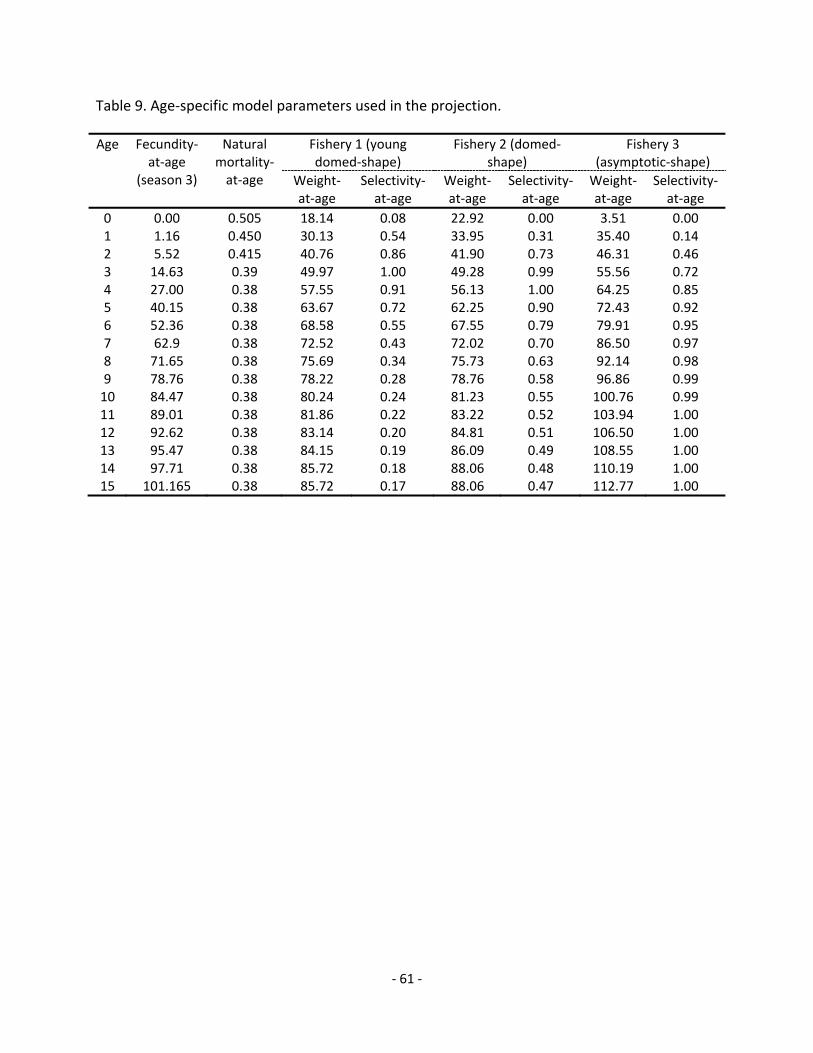
‐ 61 ‐

Table 9. Age‐specific model parameters used in the projection.

Age Fecundity‐at‐age

(season 3)

Natural mortality‐at‐age

Fishery 1 (young domed‐shape)

Fishery 2 (domed‐shape)

Fishery 3 (asymptotic‐shape)

Weight‐at‐age

Selectivity‐at‐age

Weight‐at‐age


Weight‐at‐age


0 0.00 0.505 18.14 0.08 22.92 0.00 3.51 0.00 1 1.16 0.450 30.13 0.54 33.95 0.31 35.40 0.14 2 5.52 0.415 40.76 0.86 41.90 0.73 46.31 0.46 3 14.63 0.39 49.97 1.00 49.28 0.99 55.56 0.72 4 27.00 0.38 57.55 0.91 56.13 1.00 64.25 0.85 5 40.15 0.38 63.67 0.72 62.25 0.90 72.43 0.92 6 52.36 0.38 68.58 0.55 67.55 0.79 79.91 0.95 7 62.9 0.38 72.52 0.43 72.02 0.70 86.50 0.97 8 71.65 0.38 75.69 0.34 75.73 0.63 92.14 0.98 9 78.76 0.38 78.22 0.28 78.76 0.58 96.86 0.99 10 84.47 0.38 80.24 0.24 81.23 0.55 100.76 0.99 11 89.01 0.38 81.86 0.22 83.22 0.52 103.94 1.00 12 92.62 0.38 83.14 0.20 84.81 0.51 106.50 1.00 13 95.47 0.38 84.15 0.19 86.09 0.49 108.55 1.00 14 97.71 0.38 85.72 0.18 88.06 0.48 110.19 1.00 15 101.165 0.38 85.72 0.17 88.06 0.47 112.77 1.00

‐ 62 ‐

Table 10. Decision table of projected percentiles of relative spawning stock biomass in 2017 relative to 2012 ( / ) for

alternative states of nature (columns) and harvest scenarios (rows). Fishing intensity ( %) alternatives are based on 12% (average

2001‐2003), 14% (average 2007‐2009 defined as current), 17.8% (MSY level), 20%, 30% and 100% (no fishing). Catch alternatives are

based on the 80% of average catches during 2007‐2009 (2,500 mt) and 80% of average catches during 2000‐2003 (3,600 mt). Red

blocks indicate the declining trend of SB in 2017 from 2012 where / is less than one.

Run Harvest scenario Recent recruitment ( ) Beverton‐Holt spawner‐recruit relation (SR)

5th 25th 50th 75th 95th 5th 25th 50th 75th 95th

1 % 0.72 0.87 0.98 1.06 1.18 0.66 0.88 1.06 1.25 1.52

2 % 0.85 1.03 1.14 1.23 1.36 0.83 1.09 1.29 1.51 1.82

3 = . % 1.12 1.32 1.45 1.55 1.69 1.14 1.47 1.72 1.98 2.34

4 % 1.26 1.48 1.62 1.72 1.88 1.32 1.68 1.95 2.24 2.62

5 % 1.90 2.18 2.35 2.48 2.68 2.08 2.56 2.91 3.28 3.79

6 No fishing = % 4.93 5.49 5.82 6.06 6.47 5.43 6.33 7.07 7.81 8.72

7 Catch = 2,500 mt 1.41 1.97 2.33 2.67 3.10 1.63 2.49 3.23 4.03 5.28

8 Catch = 3,600 mt 0.98 1.18 1.48 1.80 2.25 1.05 1.51 2.20 3.01 4.37

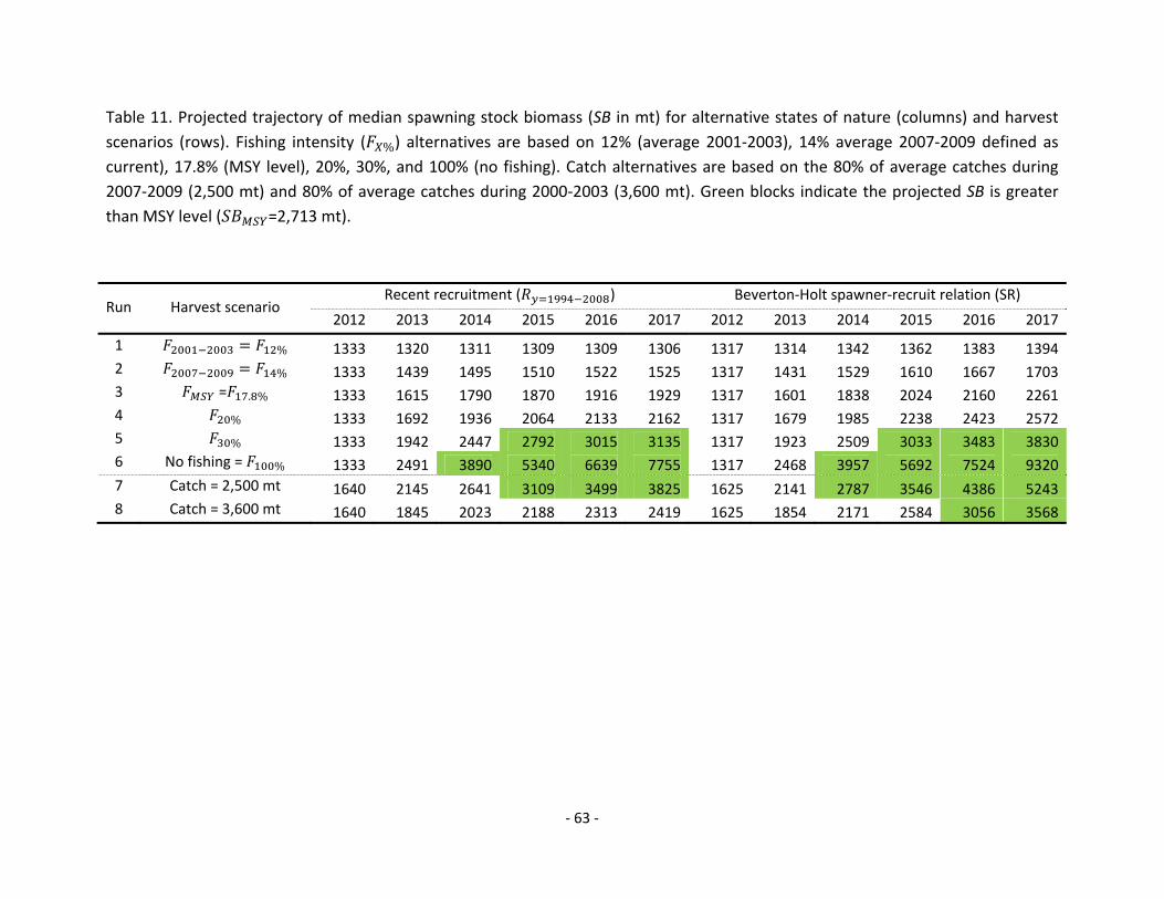
‐ 63 ‐

Table 11. Projected trajectory of median spawning stock biomass (SB in mt) for alternative states of nature (columns) and harvest

scenarios (rows). Fishing intensity ( %) alternatives are based on 12% (average 2001‐2003), 14% average 2007‐2009 defined as

current), 17.8% (MSY level), 20%, 30%, and 100% (no fishing). Catch alternatives are based on the 80% of average catches during

2007‐2009 (2,500 mt) and 80% of average catches during 2000‐2003 (3,600 mt). Green blocks indicate the projected SB is greater

than MSY level ( =2,713 mt).


2012 2013 2014 2015 2016 2017 2012 2013 2014 2015 2016 2017

1 % 1333 1320 1311 1309 1309 1306 1317 1314 1342 1362 1383 13942 % 1333 1439 1495 1510 1522 1525 1317 1431 1529 1610 1667 17033 = . % 1333 1615 1790 1870 1916 1929 1317 1601 1838 2024 2160 22614 % 1333 1692 1936 2064 2133 2162 1317 1679 1985 2238 2423 25725 % 1333 1942 2447 2792 3015 3135 1317 1923 2509 3033 3483 38306 No fishing = % 1333 2491 3890 5340 6639 7755 1317 2468 3957 5692 7524 9320

7 Catch = 2,500 mt 1640 2145 2641 3109 3499 3825 1625 2141 2787 3546 4386 52438 Catch = 3,600 mt 1640 1845 2023 2188 2313 2419 1625 1854 2171 2584 3056 3568

‐ 64 ‐

Table 12. Projected trajectory of catch (mt) for alternative states of nature (columns) and harvest scenarios (rows). Fishing intensity

( %) alternatives are based on 12% (average 2001‐2003), 14% (average 2007‐2009 defined as current), 17.8% (MSY level), 20%, 30%,

and 100% (no fishing). Catch alternatives are based on the 80% of average catches during 2007‐2009 (2,500 mt) and 80% of average

catches during 2000‐2003 (3,600 mt).


2012 2013 2014 2015 2016 2017 2012 2013 2014 2015 2016 2017

1 % 4471 4403 4378 4402 4399 4376 4373 4431 4520 4586 4588 46482 % 3974 4113 4201 4240 4246 4224 3884 4154 4374 4543 4652 47453 = . % 3267 3649 3868 3948 3971 3962 3195 3685 4066 4374 4583 47404 % 2955 3412 3663 3782 3818 3819 2890 3441 3878 4232 4491 46805 % 2001 2559 2912 3108 3187 3220 1957 2574 3103 3533 3881 41396 No fishing = % 0 0 0 0 0 0 0 0 0 0 0 0

7 Catch = 2,500 mt 2500 2500 2500 2500 2500 2500 2500 2500 2500 2500 2500 25008 Catch = 3,600 mt 3600 3600 3600 3600 3600 3600 3600 3600 3600 3600 3600 3600

‐ 65 ‐

FIGURES

Figure 1. Stock boundary delineated for the 2011 stock assessment of western and central north Pacific striped marlin (WCNPO) indicating by the red lines. The dash lines indicate the eastern Pacific Ocean stock boundary.

‐ 66 ‐

Figure 2. Available temporal coverage and sources of catch, CPUE and length composition for

the western and central north Pacific striped marlin. Assessment model used the data after

1975 indicated by the dash line.

‐ 67 ‐

Figure 3. Total annual catch of the western and central north Pacific striped marlin by all

countries (upper panel) and all gears (lower panel) harvesting the stock, 1952‐2010, where

catch data in 2010 were considered preliminary. The Other category in (a) includes catches

reported to the WCPFC by the Philippines, Indonesia, China, Vanuatu, Contains Federated

States of Micronesia, and Belize. The Other category in (b) refers to miscellaneous gears

including bait, net, trap, coastal fisheries and WCPFC catch.

0

2000

4000

6000

8000

10000

12000

1952 1960 1968 1976 1984 1992 2000 2008

Annual catch (mt)

(a) Catch by country

Japan USA Taiwan Korea Other

0

2000

4000

6000

8000

10000

12000

1952 1960 1968 1976 1984 1992 2000 2008

Annual catch (mt)

(b) Catch by gear

Longline Driftnet Harpoon Other

‐ 68 ‐

Figure 4. Time series of annual standardized CPUE indices for the Japan longline fisheries (top panel), Taiwan and Hawaii‐based longline fisheries (middle panel), and Japan driftnet fisheries (bottom panel) for the western and central north Pacific striped marlin described in Table 1. Index values in the figures are re‐scaled by the mean of each index for comparison purposes. See Table 2 for index descriptions.

0

0.4

0.8

1.2

1.6

2

2.4

1970 1980 1990 2000 2010

Stan

dardized CPUE

S1 S2 S3 S4 S5

S6 S7 S8 S9 S10

0

0.4

0.8

1.2

1.6

2

2.4

1970 1980 1990 2000 2010

Stan

dardized CPUE

S13 S14 S15

0

0.4

0.8

1.2

1.6

2

2.4

1970 1980 1990 2000 2010

Stan

dardized CPUE

S11 S12

‐ 69 ‐

Figure 5. Aggregated seasonal length compositions used in the assessment (F1, F2, F3, F4, F5, F11, F12, F13, F16, F17 and F18). Length compositions from other fisheries are not available for the assessment and length selectivity for these fisheries are mirrored to one of the fisheries in this figure.

‐ 70 ‐

Figure 6. Quarterly length compositions of fisheries used in the assessment (F1, F2, F3, F4, F5, F11, F12, F13, F16, F17 and F18 – see Table 1). Size of circles is proportional to the number of observations. Length composition data from other fisheries are not available for the assessment and selectivity patterns for these fisheries are mirrored to fisheries with length composition data.

‐ 71 ‐

Figure 6. Continued.

‐ 72 ‐


‐ 73 ‐

Figure 7. Plot of the BILLWG accepted length at age based on Sun et al. (2011) (solid line) and

the inputted representation of that in the SS model (large dash).

0

50

100

150

200

250

0 3 6 9 12 15

Eye fork length (cm

)

Age (yr)

Sun et al. 2011

input

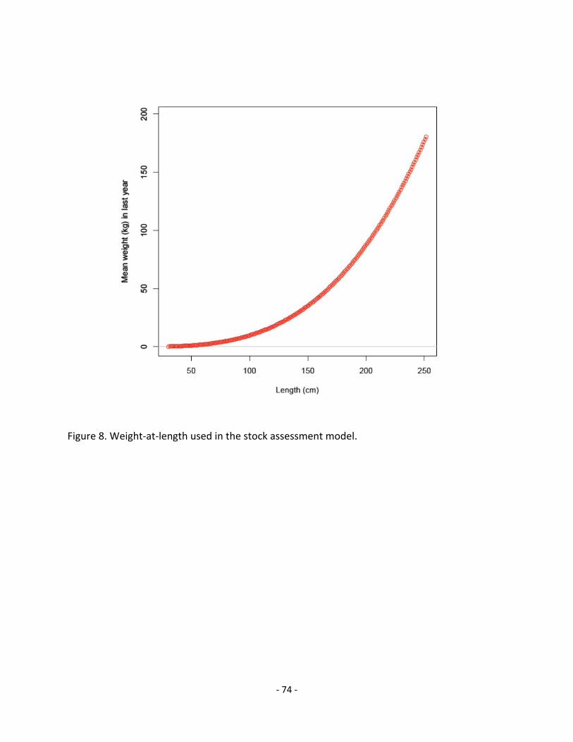
‐ 74 ‐

Figure 8. Weight‐at‐length used in the stock assessment model.

‐ 75 ‐

Figure 9. Natural mortality‐at‐age assumed in the population dynamics model.

‐ 76 ‐

Figure 10. Maturity‐at‐length (eye fork length) for female WCNPO striped marlin used in the

stock assessment model where the size‐at‐50%‐maturity was 177 cm.

‐ 77 ‐

Figure 11. Coefficient of variation (CV) of estimated recruitment from 1970‐2010.

0

0.1

0.2

0.3

0.4

0.5

0.6

0.7

1970 1975 1980 1985 1990 1995 2000 2005 2010

CV of recruitment estim

ates

‐ 78 ‐

Figure 12. Plot of estimated R0 (y‐axis) and total ending likelihood (x‐axis) for random starting values of the model (diamonds) and the base model (circle).

6.31

6.311

6.312

6.313

6.314

6.315

6.316

6.317

6.318

6.319

6.32

3948 3950 3952 3954 3956 3958

R0in log space

Total likelohood

‐ 79 ‐

A. Indices contributed to the total likelihood and were influential to the dynamics (r.m.s.e < 0.4 see Table 6).

Figure 13. Model fits to the standardized CPUE data from different fisheries used in the assessment. The blue line is the model

predicted value and the open circles are observed (data) values. The vertical lines represent the estimated confidence intervals (± 2

standard deviations) around the CPUE values. The numbers in the panels correspond to the index numbers in Table 2.

S1_JPN_DWLL1 S3_JPN_DWLL1 S7_JPN_DWLL3

S8_JPN_DWLL3 S10_JPN_CLL S14_TWN_LL (late)

‐ 80 ‐

B. Indices contributed to the total likelihood and were not influential to the dynamics (r.m.s.e > 0.4 see Table 6).


S2_JPN_DWLL1 S4_JPN_DWLL2 S5_JPN_DWLL2

S6_JPN_DWLL2 S9_JPN_DWLL3 S15_HW_LL

‐ 81 ‐

C. Indices did not contribute to the total likelihood.


S11_JPN_DRIFT S12_JPN_DRIFT S13_TWN_LL (early)

‐ 82 ‐

Figure 14. Comparison of observed (gray shaded area) and model predicted (red line) length compositions for fisheries used in the WCNPO striped marlin stock assessment (F1, F2, F3, F4, F5, F11, F12, F13, F16 F17 and F18 – see Table 1 and Figure 2 for temporal coverage of these fisheries).

‐ 83 ‐

Figure 15. Pearson residual plots of model fits to the length‐composition data for the WCNPO striped marlin fisheries used in the assessment model (F1, F2, F3, F4, F5, F11, F12, F13, F16, F17, and F18 – see Table 1 and Figure 2 for temporal coverage of these fisheries). The filled and hollow blue circles represent observations that are higher and lower than the model predictions, respectively. The areas of the circles are proportional to the absolute values of the residuals.

‐ 84 ‐


‐ 85 ‐


‐ 86 ‐

Figure 16. Length selectivity of fisheries estimated by the WCNPO striped marlin assessment model: (A) Longline fisheries: F1 (red solid line), F4 (green dotted line), and F16 (blue dashed line); (B)‐(C) Time varying longline fisheries: F2 and F3 where red solid lines are during early period, green dotted lines are during mid period, and blue dashed lines are during late period; (D) Domed shape fishery (F12) (red solid line); (E) Asymptotic fisheries: F5 (red solid line) and F11 (green dotted line); (F) Asymptotic fisheries: F13 (red solid line) and F17 (green dotted line). See Table 1 for fishery definitions.

0

0.2

0.4

0.6

0.8

1

0 50 100 150 200 250

Selectivity

Length (cm)

A. Longline fisheries

F1

F4

F16

0

0.2

0.4

0.6

0.8

1

0 50 100 150 200 250

Selectivity

Length (cm)

D. Domed shape fishery

F12

0

0.2

0.4

0.6

0.8

1

0 50 100 150 200 250

Selectivity

Length (cm)

B. Longline fisheries

F2_early

F2_mid

F2_late

0

0.2

0.4

0.6

0.8

1

0 50 100 150 200 250

Selectivity

Length (cm)

E. Asymptotic fisheries

F5

F11

0

0.2

0.4

0.6

0.8

1

0 50 100 150 200 250

Selectivity

Length (cm)

C. Longline fisheries

F3_early

F3_mid

F3_late

0

0.2

0.4

0.6

0.8

1

0 50 100 150 200 250

Selectivity

Length (cm)

F. Asymptotic fisheries

F13

F17

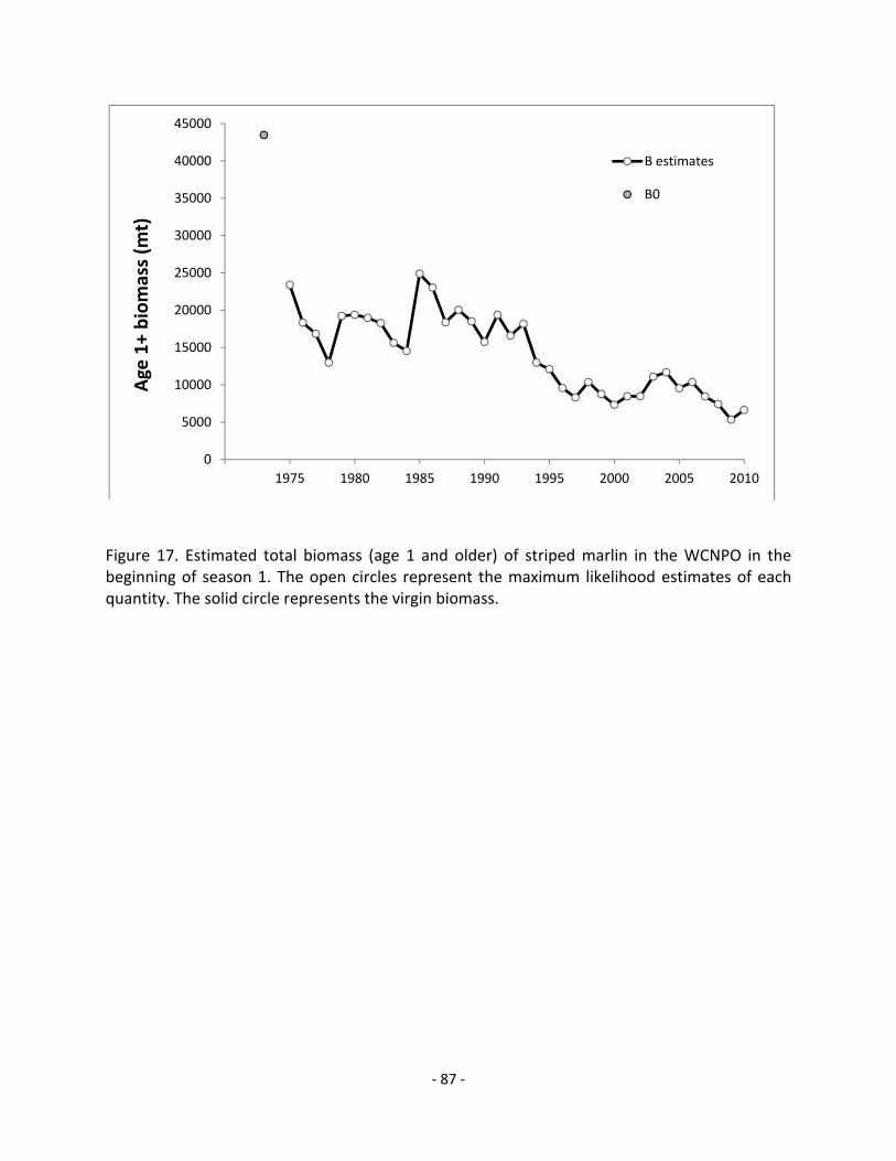
‐ 87 ‐

Figure 17. Estimated total biomass (age 1 and older) of striped marlin in the WCNPO in the beginning of season 1. The open circles represent the maximum likelihood estimates of each quantity. The solid circle represents the virgin biomass.

0

5000

10000

15000

20000

25000

30000

35000

40000

45000

1970 1975 1980 1985 1990 1995 2000 2005 2010

Age 1+ biomass (m

t)B estimates

B0

‐ 88 ‐

Figure 18. Estimated spawning biomass (SB) of striped marlin in the WCNPO. The solid line with open circles represents the maximum likelihood estimates of quantity and the dotted lines are the 95% asymptotic intervals of the estimates (± 2 standard deviations), where the dashed horizontal line is the estimate of spawning biomass at MSY level ( ). The solid circle represents the virgin spawning biomass and associated 95% confidence intervals. Since spawning occurs in the beginning of season 2 (beginning of spawning cycle), there is one annual estimate of spawning biomass.

0

2000

4000

6000

8000

10000

12000

14000

16000

18000

20000

1970 1975 1980 1985 1990 1995 2000 2005 2010

Spaw

ning biomass (m

t)95% CI

5% CI

SB estimtes

SBmsy

SB0

95% CI of SB0

5% CI of SB0

‐ 89 ‐

Figure 19. Estimated age‐0 recruitment of striped marlin in the WCNPO. The open circles represent the maximum likelihood estimates of quantity and the solid circle represents the virgin recruit. The vertical bars are the 95% asymptotic intervals of the estimates (± 2 standard deviations). Since recruitment timing occurs in season 3, there is one annual estimate of recruitment.

0

200

400

600

800

1000

1200

1400

1600

1800

2000

1970 1975 1980 1985 1990 1995 2000 2005 2010

Recruitment (1,000 s)

95% CI

5% CI

Estimates

‐ 90 ‐

Figure 20. Estimated fishing mortality (average F across age 3 and older) of striped marlin in the WCNPO. The solid line represents the maximum likelihood estimates of quantity and the dotted lines are the 95% asymptotic intervals of the estimates (± 2 standard deviations), where the dashed horizontal line is the estimate of fishing mortality at MSY level ( ).

0

0.2

0.4

0.6

0.8

1

1.2

1.4

1.6

1.8

1975 1980 1985 1990 1995 2000 2005 2010Fishing mortality (average, age‐3 and older)

95% CI 5% CI F estimates Fmsy

‐ 91 ‐

Figure 21. Estimated spawning potential ratio (SPR) of striped marlin in the WCNPO. The solid line represents the maximum likelihood estimates of quantity and the dotted lines are the 95% asymptotic intervals of the estimates (± 2 standard deviations), where the dashed horizontal line is the estimate of fishing mortality at MSY level ( ).

0

0.05

0.1

0.15

0.2

0.25

1975 1980 1985 1990 1995 2000 2005 2010

Spaw

ning potential ratio

95% CI 5% CI SPR estimates SPRmsy

‐ 92 ‐

Figure 22. Sensitivity analysis for alternative JPN_DWLL CPUE series. Panel A presents the alternative time series of annual standardized CPUE indices for the Japan longline fisheries. Panel B and C present the trajectory of total biomass and spawning potential ratio (SPR) respectively.

0

0.005

0.01

0.015

0.02

0.025

0.03

0.035

1970 1980 1990 2000 2010

Stan

dardized CPUE

A. Alternative JPN_DWLL CPUE

0

5000

10000

15000

20000

25000

30000

1970 1980 1990 2000 2010

Age1+ biomass (m

t)

B. Age 1+ biomassBase case

Alternative CPUE

0

0.05

0.1

0.15

0.2

0.25

1970 1980 1990 2000 2010

SPR

C. SPR Base case

Alternative CPUE

‐ 93 ‐

Figure 23. Sensitivity analyses for dropping CPUE for poor fit fishery, JPN_DWLL2 or HW_LL. Panel A and B present the trajectory of total biomass and spawning potential ratio (SPR) respectively.

0

5000

10000

15000

20000

25000

30000

1970 1975 1980 1985 1990 1995 2000 2005 2010

Age1+ biomass (m

t)

A. Age 1+ biomass

Base case

exclude JPN_DWLL2

exclude HW_LL

0

0.05

0.1

0.15

0.2

0.25

1970 1975 1980 1985 1990 1995 2000 2005 2010

SPR

B. SPR Base case

exclude JPN_DWLL2

exclude HW_LL

‐ 94 ‐

Figure 24. Sensitivity analyses for alternative natural mortality (M). Panel A presents the alternative natural mortality schedules, high adult M at 0.5 year‐1 and low adult M at 0.3 year‐1. Panel B and C present the trajectory of total biomass and spawning potential ratio (SPR) respectively.

0

0.2

0.4

0.6

0.8

1

0 2 4 6 8 10 12 14

Natural M

ortality

Age

A. Natural mortalityBase case

High M

Low M

0

5000

10000

15000

20000

25000

30000

35000

1970 1980 1990 2000 2010

Age1+ biomass (m

t)

B. Age 1+ biomassBase case

High M

Low M

0

0.05

0.1

0.15

0.2

0.25

0.3

0.35

1970 1980 1990 2000 2010

SPR

C. SPR Base case

High M

Low M

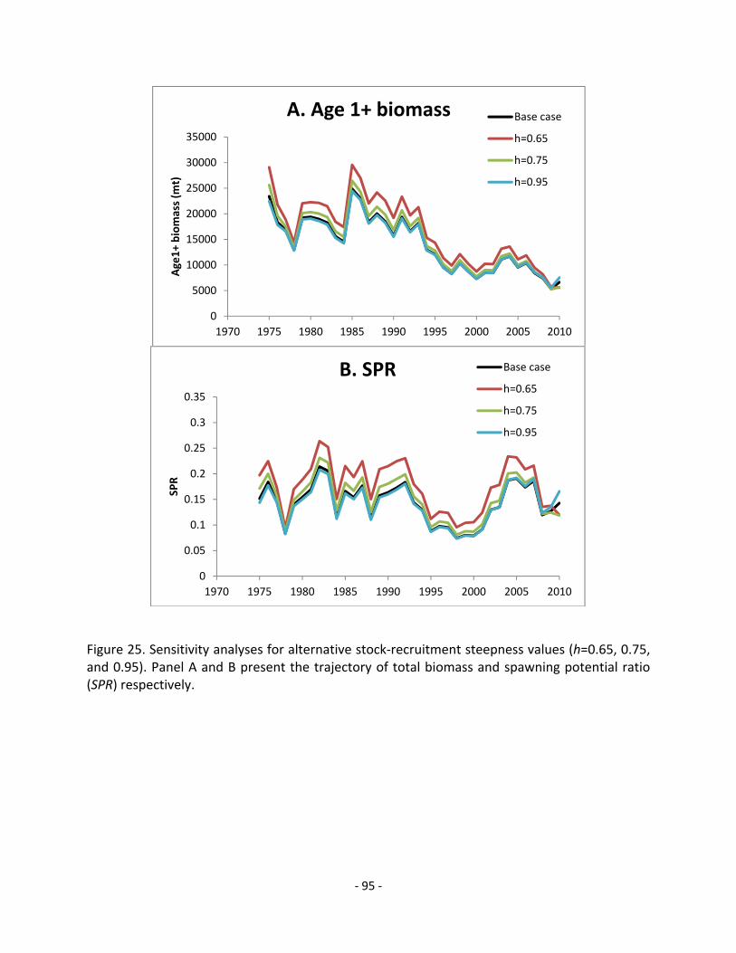
‐ 95 ‐

Figure 25. Sensitivity analyses for alternative stock‐recruitment steepness values (h=0.65, 0.75, and 0.95). Panel A and B present the trajectory of total biomass and spawning potential ratio (SPR) respectively.

0

5000

10000

15000

20000

25000

30000

35000

1970 1975 1980 1985 1990 1995 2000 2005 2010

Age1+ biomass (m

t)

A. Age 1+ biomass Base case

h=0.65

h=0.75

h=0.95

0

0.05

0.1

0.15

0.2

0.25

0.3

0.35

1970 1975 1980 1985 1990 1995 2000 2005 2010

SPR

B. SPR Base case

h=0.65

h=0.75

h=0.95

‐ 96 ‐

Figure 26. Sensitivity analyses for alternative growth curves. Panel A presents the alternative

growth curve, larger size for adult or smaller size for adult. Panel B and C present the trajectory of

total biomass and spawning potential ratio (SPR) respectively.

0

50

100

150

200

250

0 2 4 6 8 10 12 14

Eye fork length (cm

)

Age

A. Growth curve

Base case

Larger fish

Smaller fish

0

5000

10000

15000

20000

25000

30000

1970 1980 1990 2000 2010

Age1+ biomass (m

t)

B. Age 1+ biomass

Base case

Larger_fish

Smaller_fish

0

0.05

0.1

0.15

0.2

0.25

1970 1980 1990 2000 2010

SPR

C. SPR Base case

Larger_fish

Smaller_fish

‐ 97 ‐

Figure 27. Sensitivity analysis for larger CV of the length at age for older fish (CV=12%). Panel A and B present the trajectory of total biomass and spawning potential ratio (SPR) respectively.

0

5000

10000

15000

20000

25000

30000

1970 1975 1980 1985 1990 1995 2000 2005 2010

Age1+ biomass (m

t)

A. Age 1+ biomass

Base case

CVold_0.12

0

0.05

0.1

0.15

0.2

0.25

1970 1975 1980 1985 1990 1995 2000 2005 2010

SPR

B. SPRBase case

CVold_0.12

‐ 98 ‐

Figure 28. Sensitivity analysis for using assumptions from the 2007 assessment model with catch, CPUE, and length composition data from the current base model. Panel A and B present the trajectory of total biomass and spawning potential ratio (SPR) respectively.

0

5000

10000

15000

20000

25000

30000

35000

1970 1975 1980 1985 1990 1995 2000 2005 2010

Age1+ biomass (m

t)

A. Age 1+ biomass

Base case

Like 2007 assessment

0

0.05

0.1

0.15

0.2

0.25

1970 1975 1980 1985 1990 1995 2000 2005 2010

SPR

B. SPRBase case

Like 2007 assessment

‐ 99 ‐

Figure 29. Sensitivity analysis for including the catch from 1952 to 1974. Panel A and B present the trajectory of total biomass and spawning potential ratio (SPR) respectively.

0

5000

10000

15000

20000

25000

30000

35000

1940 1950 1960 1970 1980 1990 2000 2010

Age1+ biomass (m

t)

A. Age 1+ biomass

Base case

Start1952

0

0.1

0.2

0.3

0.4

0.5

0.6

1940 1950 1960 1970 1980 1990 2000 2010

SPR

B. SPRBase case

Start1952

‐ 100 ‐

Figure 30. Historical trends in recruitment of WCNPO striped marlin (age‐0) estimated by the SS3 base‐case model and the assumed periods of low recruitments used for future projection scenarios.

0

200

400

600

800

1000

1200

1400

1600

1800

1975 1980 1985 1990 1995 2000 2005 2010

Age

‐0 recruits (1,000s)

Time series 1975‐2010

High recruitment period

Low recruitment period

‐ 101 ‐

Figure 31. Kobe plot of the trends in estimates of relative fishing mortality and spawning biomass of Western and Central North Pacific striped marlin (Kajikia audax) during 1975‐2010.

‐ 102 ‐

Figure 32. Kobe plot of the trends in estimates of relative fishing intensity and spawning biomass of

Western and Central North Pacific striped marlin (Kajikia audax) during 1975‐2010.

‐ 103 ‐

Appendix A

SS3 starter file used in the WCNPO striped marlin assessment for the base case.

#C starter comment here SM_data.ss SM_control.ss 0 # 0=use init values in control file; 1=use ss3.par 1 # run display detail (0,1,2) 1 # detailed age-structured reports in REPORT.SSO (0,1) 1 # write detailed checkup.sso file (0,1) 0 # write parm values to ParmTrace.sso (0=no,1=good,active; 2=good,all; 3=every_iter,all_parms; 4=every,active) 1 # write to cumreport.sso (0=no,1=like&timeseries; 2=add survey fits) 0 # Include prior_like for non-estimated parameters (0,1) 1 # Use Soft Boundaries to aid convergence (0,1) (recommended) 1 # Number of bootstrap datafiles to produce 10 # Turn off estimation for parameters entering after this phase 10 # MCeval burn interval 2 # MCeval thin interval 0 # jitter initial parm value by this fraction -1 # min yr for sdreport outputs (-1 for styr) -1 # max yr for sdreport outputs (-1 for endyr; -2 for endyr+Nforecastyrs 0 # N individual STD years #vector of year values 0.0001 # final convergence criteria (e.g. 1.0e-04) 0 # retrospective year relative to end year (e.g. -4) 1 # min age for calc of summary biomass 1 # Depletion basis: denom is: 0=skip; 1=rel X*B0; 2=rel X*Bmsy; 3=rel X*B_styr 1 # Fraction (X) for Depletion denominator (e.g. 0.4) 4 # SPR_report_basis: 0=skip; 1=(1-SPR)/(1-SPR_tgt); 2=(1-SPR)/(1-SPR_MSY); 3=(1-SPR)/(1-SPR_Btarget); 4=rawSPR (1-SPR) 4 # F_report_units: 0=skip; 1=exploitation(Bio); 2=exploitation(Num); 3=sum(Frates); 4=F for range of ages 3 13 #_min and max age over which average F will be calculated with F_reporting=4 0 # F_report_basis: 0=raw; 1=F/Fspr; 2=F/Fmsy ; 3=F/Fbtgt 999 # check value for end of file

‐ 104 ‐

Appendix A

SS3 forecast file used in the WCNPO striped marlin assessment for the base case.

#V3.20b #C generic forecast file # for all year entries except rebuilder; enter either: actual year, -999 for styr, 0 for endyr, neg number for rel. endyr 1 # Benchmarks: 0=skip; 1=calc F_spr,F_btgt,F_msy 2 # MSY: 1= set to F(SPR); 2=calc F(MSY); 3=set to F(Btgt); 4=set to F(endyr) 0.4 # SPR target (e.g. 0.40) 0.4 # Biomass target (e.g. 0.40) #_Bmark_years: beg_bio, end_bio, beg_selex, end_selex, beg_relF, end_relF (enter actual year, or values of 0 or -integer to be rel. endyr) 0 0 0 0 0 0 # 2001 2001 2001 2001 2001 2001 # after processing 1 #Bmark_relF_Basis: 1 = use year range; 2 = set relF same as forecast below # 0 # Forecast: 0=none; 1=F(SPR); 2=F(MSY) 3=F(Btgt); 4=Ave F (uses first-last relF yrs); 5=input annual F scalar 1 # N forecast years 0.2 # F scalar (only used for Do_Forecast==5) #_Fcast_years: beg_selex, end_selex, beg_relF, end_relF (enter actual year, or values of 0 or -integer to be rel. endyr) 0 0 0 0 # 2001 2001 1991 2001 # after processing 1 # Control rule method (1=catch=f(SSB) west coast; 2=F=f(SSB) ) 0.4 # Control rule Biomass level for constant F (as frac of Bzero, e.g. 0.40) 0.1 # Control rule Biomass level for no F (as frac of Bzero, e.g. 0.10) 0.75 # Control rule target as fraction of Flimit (e.g. 0.75) 3 #_N forecast loops (1-3) (fixed at 3 for now) 3 #_First forecast loop with stochastic recruitment 0 #_Forecast loop control #3 (reserved for future bells&whistles) 0 #_Forecast loop control #4 (reserved for future bells&whistles) 0 #_Forecast loop control #5 (reserved for future bells&whistles) 2010 #FirstYear for caps and allocations (should be after years with fixed inputs) 0.05 # stddev of log(realized catch/target catch) in forecast (set value>0.0 to cause active impl_error) 0 # Do West Coast gfish rebuilder output (0/1) 1999 # Rebuilder: first year catch could have been set to zero (Ydecl)(-1 to set to 1999) 2002 # Rebuilder: year for current age structure (Yinit) (-1 to set to endyear+1) 1 # fleet relative F: 1=use first-last alloc year; 2=read seas(row) x fleet(col) below # Note that fleet allocation is used directly as average F if Do_Forecast=4 2 # basis for fcast catch tuning and for fcast catch caps and allocation (2=deadbio; 3=retainbio; 5=deadnum; 6=retainnum) # Conditional input if relative F choice = 2 # Fleet relative F: rows are seasons, columns are fleets #_Fleet: FISHERY1 # 1 # max totalcatch by fleet (-1 to have no max) -1 # max totalcatch by area (-1 to have no max) -1 # fleet assignment to allocation group (enter group ID# for each fleet, 0 for not included in an alloc group) 0 #_Conditional on >1 allocation group # allocation fraction for each of: 0 allocation groups # no allocation groups 0 # Number of forecast catch levels to input (else calc catch from forecast F) 2 # basis for input Fcast catch: 2=dead catch; 3=retained catch; 99=input Hrate(F) (units are from fleetunits; note new codes in SSV3.20) # Input fixed catch values #Year Seas Fleet Catch(or_F) 999 # verify end of input

‐ 105 ‐

Appendix A

SS3 control file used in the WCNPO striped marlin assessment for the base case.

#V3.20b #C Striped Marlin Control file #_data_and_control_files: SM_data.ss // SM_control.ss #_SS-V3.20b-safe;_01/23/2011;_Stock_Synthesis_by_Richard_Methot_(NOAA)_using_ADMB 1 #_N_Growth_Patterns 1 #_N_Morphs_Within_GrowthPattern #_Cond 1 #_Morph_between/within_stdev_ratio (no read if N_morphs=1) #_Cond 1 #vector_Morphdist_(-1_in_first_val_gives_normal_approx) # 1 # number of recruitment assignments (overrides GP*area*seas parameter values) 0 # recruitment interaction requested #GP seas area for each recruitment assignment 1 3 1 # #_Cond 0 # N_movement_definitions goes here if N_areas > 1 #_Cond 1.0 # first age that moves (real age at begin of season, not integer) also cond on do_migration>0 #_Cond 1 1 1 2 4 10 # example move definition for seas=1, morph=1, source=1 dest=2, age1=4, age2=10 # 2 #_Nblock_Patterns 2 1 #_blocks_per_pattern # begin and end years of blocks 1987 1999 2000 2010 2001 2010 # 0.5 #_fracfemale 3 #_natM_type:_0=1Parm; 1=N_breakpoints;_2=Lorenzen;_3=agespecific;_4=agespec_withseasinterpolate #_Age_natmort_by gender x growthpattern 0.54 0.47 0.43 0.4 0.38 0.38 0.38 0.38 0.38 0.38 0.38 0.38 0.38 0.38 0.38 0.38 1 # GrowthModel: 1=vonBert with L1&L2; 2=Richards with L1&L2; 3=not implemented; 4=not implemented 0.3 #_Growth_Age_for_L1 15 #_Growth_Age_for_L2 (999 to use as Linf) 0 #_SD_add_to_LAA (set to 0.1 for SS2 V1.x compatibility) 0 #_CV_Growth_Pattern: 0 CV=f(LAA); 1 CV=F(A); 2 SD=F(LAA); 3 SD=F(A) 1 #_maturity_option: 1=length logistic; 2=age logistic; 3=read age-maturity matrix by growth_pattern; 4=read age-fecundity; 5=read fec and wt from wtatage.ss #_placeholder for empirical age-maturity by growth pattern 1 #_First_Mature_Age 1 #_fecundity option:(1)eggs=Wt*(a+b*Wt);(2)eggs=a*L^b;(3)eggs=a*Wt^b 0 #_hermaphroditism option: 0=none; 1=age-specific fxn 1 #_parameter_offset_approach (1=none, 2= M, G, CV_G as offset from female-GP1, 3=like SS2 V1.x) 1 #_env/block/dev_adjust_method (1=standard; 2=logistic transform keeps in base parm bounds; 3=standard w/ no bound check) # #_growth_parms #_LO HI INIT PRIOR PR_type SD PHASE env-var use_dev dev_minyr dev_maxyr dev_stddev Block Block_Fxn 10 160 104 40.2 -1 99 -4 0 0 0 0 0 0 0 # L_at_Amin_Fem_GP_1 110 260 214 146.46 -1 99 -3 0 0 0 0 0 0 0 # L_at_Amax_Fem_GP_1 0.01 0.56 0.24 0.149 -1 99 -4 0 0 0 0 0 0 0 # VonBert_K_Fem_GP_1 0.01 0.3 0.14 0.135 -1 99 -3 0 0 0 0 0 0 0 # CV_young_Fem_GP_1 0.01 0.3 0.08 0.05 -1 99 -3 0 0 0 0 0 0 0 # CV_old_Fem_GP_1 -2 2 4.68e-006 8.7e-005 -1 99 -3 0 0 0 0 0 0 0 # Wtlen_1_Fem -2 4 3.16 3.16 -1 99 -3 0 0 0 0 0 0 0 # Wtlen_2_Fem 1 200 177 5 -1 99 -3 0 0 0 0 0 0 0 # Mat50%_Fem -5 5 -0.064 -0.052 -1 99 -3 0 0 0 0 0 0 0 # Mat_slope_Fem 0 3 1 1 -1 99 -3 0 0 0 0 0 0 0 # Eggs/kg_inter_Fem 0 3 0 0 -1 99 -3 0 0 0 0 0 0 0 # Eggs/kg_slope_wt_Fem -4 4 0 1 -1 99 -3 0 0 0 0 0 0 0 # RecrDist_GP_1 -4 4 0 1 -1 99 -3 0 0 0 0 0 0 0 # RecrDist_Area_1 -4 4 -4 1 -1 99 -3 0 0 0 0 0 0 0 # RecrDist_Seas_1 -4 4 -4 1 -1 99 -3 0 0 0 0 0 0 0 # RecrDist_Seas_2 -4 4 -4 1 -1 99 -3 0 0 0 0 0 0 0 # RecrDist_Seas_3

‐ 106 ‐

-4 4 -4 1 -1 99 -3 0 0 0 0 0 0 0 # RecrDist_Seas_4 -4 4 1 1 -1 99 -3 0 0 0 0 0 0 0 # CohortGrowDev # #_Cond 0 #custom_MG-env_setup (0/1) #_Cond -2 2 0 0 -1 99 -2 #_placeholder when no MG-environ parameters # #_Cond 0 #custom_MG-block_setup (0/1) #_Cond -2 2 0 0 -1 99 -2 #_placeholder when no MG-block parameters #_Cond No MG parm trends # #_seasonal_effects_on_biology_parms 0 0 0 0 0 0 0 0 0 0 #_femwtlen1,femwtlen2,mat1,mat2,fec1,fec2,Malewtlen1,malewtlen2,L1,K #_Cond -2 2 0 0 -1 99 -2 #_placeholder when no seasonal MG parameters # #_Cond -4 #_MGparm_Dev_Phase # #_Spawner-Recruitment 3 #_SR_function: 1=B-H_flattop; 2=Ricker; 3=std_B-H; 4=SCAA; 5=Hockey; 6=Shepard_3Parm #_LO HI INIT PRIOR PR_type SD PHASE 3 15 6.31642 10 -1 99 1 # SR_R0 0.2 1 0.87 0.75 -1 99 -4 # SR_steep 0 2 0.6 0.6 -1 99 -1 # SR_sigmaR -5 5 0 0 -1 99 -1 # SR_envlink -10 10 0 0 -1 99 -1 # SR_R1_offset 0 0 0 0 -1 99 -1 # SR_autocorr 0 #_SR_env_link 0 #_SR_env_target_0=none;1=devs;_2=R0;_3=steepness 1 #do_recdev: 0=none; 1=devvector; 2=simple deviations 1970 # first year of main recr_devs; early devs can preceed this era 2008 # last year of main recr_devs; forecast devs start in following year 2 #_recdev phase 0 # (0/1) to read 13 advanced options #_Cond 0 #_recdev_early_start (0=none; neg value makes relative to recdev_start) #_Cond -4 #_recdev_early_phase #_Cond 0 #_forecast_recruitment phase (incl. late recr) (0 value resets to maxphase+1) #_Cond 1 #_lambda for Fcast_recr_like occurring before endyr+1 #_Cond 975 #_last_early_yr_nobias_adj_in_MPD #_Cond 1960 #_first_yr_fullbias_adj_in_MPD #_Cond 2008 #_last_yr_fullbias_adj_in_MPD #_Cond 2011 #_first_recent_yr_nobias_adj_in_MPD #_Cond 1 #_max_bias_adj_in_MPD (-1 to override ramp and set biasadj=1.0 for all estimated recdevs) #_Cond 0 #_period of cycles in recruitment (N parms read below) #_Cond -5 #min rec_dev #_Cond 5 #max rec_dev #_Cond 0 #_read_recdevs #_end of advanced SR options # #_placeholder for full parameter lines for recruitment cycles # read specified recr devs #_Yr Input_value # # all recruitment deviations #DisplayOnly -0.824592 # Main_InitAge_5 #DisplayOnly -0.852135 # Main_InitAge_4 #DisplayOnly -0.682242 # Main_InitAge_3 #DisplayOnly 0.740143 # Main_InitAge_2 #DisplayOnly -0.0334567 # Main_InitAge_1 #DisplayOnly 0.0385122 # Main_RecrDev_1975 #DisplayOnly 0.195881 # Main_RecrDev_1976 #DisplayOnly -0.380875 # Main_RecrDev_1977 #DisplayOnly 1.25908 # Main_RecrDev_1978 #DisplayOnly 0.0712119 # Main_RecrDev_1979 #DisplayOnly 0.455171 # Main_RecrDev_1980 #DisplayOnly 0.334656 # Main_RecrDev_1981 #DisplayOnly -0.559914 # Main_RecrDev_1982 #DisplayOnly 0.0803683 # Main_RecrDev_1983 #DisplayOnly 1.43229 # Main_RecrDev_1984 #DisplayOnly -0.508716 # Main_RecrDev_1985 #DisplayOnly -0.0390994 # Main_RecrDev_1986 #DisplayOnly 0.739858 # Main_RecrDev_1987 #DisplayOnly 0.397834 # Main_RecrDev_1988

‐ 107 ‐

#DisplayOnly -0.203685 # Main_RecrDev_1989 #DisplayOnly 0.863201 # Main_RecrDev_1990 #DisplayOnly -0.499496 # Main_RecrDev_1991 #DisplayOnly 0.621897 # Main_RecrDev_1992 #DisplayOnly -1.21521 # Main_RecrDev_1993 #DisplayOnly 0.306161 # Main_RecrDev_1994 #DisplayOnly -0.15937 # Main_RecrDev_1995 #DisplayOnly -0.10233 # Main_RecrDev_1996 #DisplayOnly 0.595421 # Main_RecrDev_1997 #DisplayOnly -0.0588611 # Main_RecrDev_1998 #DisplayOnly -0.0258466 # Main_RecrDev_1999 #DisplayOnly 0.492303 # Main_RecrDev_2000 #DisplayOnly 0.0983866 # Main_RecrDev_2001 #DisplayOnly 0.607559 # Main_RecrDev_2002 #DisplayOnly 0.163198 # Main_RecrDev_2003 #DisplayOnly -1.07467 # Main_RecrDev_2004 #DisplayOnly 0.204432 # Main_RecrDev_2005 #DisplayOnly -1.03525 # Main_RecrDev_2006 #DisplayOnly -0.524829 # Main_RecrDev_2007 #DisplayOnly -0.916992 # Main_RecrDev_2008 # #Fishing Mortality info 0.5 # F ballpark for tuning early phases 1970 # F ballpark year (neg value to disable) 3 # F_Method: 1=Pope; 2=instan. F; 3=hybrid (hybrid is recommended) 4 # max F or harvest rate, depends on F_Method # no additional F input needed for Fmethod 1 # if Fmethod=2; read overall start F value; overall phase; N detailed inputs to read # if Fmethod=3; read N iterations for tuning for Fmethod 3 5 # N iterations for tuning F in hybrid method (recommend 3 to 7) # #_initial_F_parms #_LO HI INIT PRIOR PR_type SD PHASE 0 1 0 0 -1 99 -1 # InitF_1JPN_DWLL1 0 1 0 0 -1 99 -2 # InitF_2JPN_DWLL2 0 1 0 0 -1 99 -2 # InitF_3JPN_DWLL3 0 1 0 0 -1 99 -2 # InitF_4JPN_CLL 0 7 1.56763 0 -1 99 1 # InitF_5JPN_DRIFT 0 1 0 0 -1 99 -2 # InitF_6JPN_OLL 0 1 0 0 -1 99 -2 # InitF_7JPN_SQUID 0 1 0 0 -1 99 -1 # InitF_8JPN_BAIT 0 1 0 0 -1 99 -2 # InitF_9JPN_NET 0 1 0 0 -1 99 -1 # InitF_10JPN_TRAP 0 1 0 0 -1 99 -1 # InitF_11JPN_OTHER_early 0 1 0 0 -1 99 -2 # InitF_12JPN_OTHER_late 0 1 0 0 -1 99 -2 # InitF_13TWN_LL 0 1 0 0 -1 99 -2 # InitF_14TWN_OSLL 0 1 0 0 -1 99 -2 # InitF_15TWN_CF 0 1 0 0 -1 99 -2 # InitF_16HW_LL 0 1 0 0 -1 99 -2 # InitF_17WCPO_OTHER 0 1 0 0 -1 99 -2 # InitF_18KOR_LL # #_Q_setup # Q_type options: <0=mirror, 0/1=float, 2=parameter, 3=parm_w_random_dev, 4=parm_w_randwalk) #_Den-dep env-var extra_se Q_type 0 0 0 0 # 1 JPN_DWLL1 0 0 0 0 # 2 JPN_DWLL2 0 0 0 0 # 3 JPN_DWLL3 0 0 0 0 # 4 JPN_CLL 0 0 0 0 # 5 JPN_DRIFT 0 0 0 0 # 6 JPN_OLL 0 0 0 0 # 7 JPN_SQUID 0 0 0 0 # 8 JPN_BAIT 0 0 0 0 # 9 JPN_NET 0 0 0 0 # 10 JPN_TRAP 0 0 0 0 # 11 JPN_OTHER_early 0 0 0 0 # 12 JPN_OTHER_late 0 0 0 0 # 13 TWN_LL 0 0 0 0 # 14 TWN_OSLL 0 0 0 0 # 15 TWN_CF 0 0 0 0 # 16 HW_LL

‐ 108 ‐

0 0 0 0 # 17 WCPO_OTHER 0 0 0 0 # 18 KOR_LL 0 0 0 0 # 19 Svey2_JPN_DWLL1 0 0 0 0 # 20 Svey3_JPN_DWLL1 0 0 0 0 # 21 Svey4_JPN_DWLL1 0 0 0 0 # 22 Svey5_JPN_DWLL2 0 0 0 0 # 23 Svey6_JPN_DWLL2 0 0 0 0 # 24 Svey7_JPN_DWLL2 0 0 0 0 # 25 Svey8_JPN_DWLL3 0 0 0 0 # 26 Svey9_JPN_DWLL3 0 0 0 0 # 27 Svey10_JPN_DWLL3 0 0 0 0 # 28 Svey11_JPN_CLL 0 0 0 0 # 29 Svey12_JPN_DFT 0 0 0 0 # 30 Svey13_JPN_DFT 0 0 0 0 # 31 Svey14_TWN_EARLY 0 0 0 0 # 32 Svey15_TWN_LATE 0 0 0 0 # 33 Svey16_HWLL # #_Cond 0 #_If q has random component, then 0=read one parm for each fleet with random q; 1=read a parm for each year of index #_Q_parms(if_any) # #_size_selex_types #_Pattern Discard Male Special 24 0 0 0 # 1 JPN_DWLL1 24 0 0 0 # 2 JPN_DWLL2 24 0 0 0 # 3 JPN_DWLL3 24 0 0 0 # 4 JPN_CLL 1 0 0 0 # 5 JPN_DRIFT 5 0 0 4 # 6 JPN_OLL 5 0 0 5 # 7 JPN_SQUID 5 0 0 4 # 8 JPN_BAIT 5 0 0 4 # 9 JPN_NET 5 0 0 4 # 10 JPN_TRAP 1 0 0 0 # 11 JPN_OTHER_early 24 0 0 0 # 12 JPN_OTHER_late 24 0 0 0 # 13 TWN_LL 5 0 0 13 # 14 TWN_OSLL 5 0 0 13 # 15 TWN_CF 24 0 0 0 # 16 HW_LL 24 0 0 0 # 17 WCPO_OTHER 5 0 0 2 # 18 KOR_LL 5 0 0 1 # 19 Svey2_JPN_DWLL1 5 0 0 1 # 20 Svey3_JPN_DWLL1 5 0 0 1 # 21 Svey4_JPN_DWLL1 5 0 0 2 # 22 Svey5_JPN_DWLL2 5 0 0 2 # 23 Svey6_JPN_DWLL2 5 0 0 2 # 24 Svey7_JPN_DWLL2 5 0 0 3 # 25 Svey8_JPN_DWLL3 5 0 0 3 # 26 Svey9_JPN_DWLL3 5 0 0 3 # 27 Svey10_JPN_DWLL3 5 0 0 4 # 28 Svey11_JPN_CLL 5 0 0 5 # 29 Svey12_JPN_DFT 5 0 0 5 # 30 Svey13_JPN_DFT 5 0 0 13 # 31 Svey14_TWN_EARLY 5 0 0 13 # 32 Svey15_TWN_LATE 5 0 0 16 # 33 Svey16_HWLL # #_age_selex_types #_Pattern ___ Male Special 11 0 0 0 # 1 JPN_DWLL1 11 0 0 0 # 2 JPN_DWLL2 11 0 0 0 # 3 JPN_DWLL3 11 0 0 0 # 4 JPN_CLL 11 0 0 0 # 5 JPN_DRIFT 11 0 0 0 # 6 JPN_OLL 11 0 0 0 # 7 JPN_SQUID 11 0 0 0 # 8 JPN_BAIT 11 0 0 0 # 9 JPN_NET 11 0 0 0 # 10 JPN_TRAP 11 0 0 0 # 11 JPN_OTHER_early

‐ 109 ‐

11 0 0 0 # 12 JPN_OTHER_late 11 0 0 0 # 13 TWN_LL 11 0 0 0 # 14 TWN_OSLL 11 0 0 0 # 15 TWN_CF 11 0 0 0 # 16 HW_LL 11 0 0 0 # 17 WCPO_OTHER 11 0 0 0 # 18 KOR_LL 11 0 0 0 # 19 Svey2_JPN_DWLL1 11 0 0 0 # 20 Svey3_JPN_DWLL1 11 0 0 0 # 21 Svey4_JPN_DWLL1 11 0 0 0 # 22 Svey5_JPN_DWLL2 11 0 0 0 # 23 Svey6_JPN_DWLL2 11 0 0 0 # 24 Svey7_JPN_DWLL2 11 0 0 0 # 25 Svey8_JPN_DWLL3 11 0 0 0 # 26 Svey9_JPN_DWLL3 11 0 0 0 # 27 Svey10_JPN_DWLL3 11 0 0 0 # 28 Svey11_JPN_CLL 11 0 0 0 # 29 Svey12_JPN_DFT 11 0 0 0 # 30 Svey13_JPN_DFT 11 0 0 0 # 31 Svey14_TWN_EARLY 11 0 0 0 # 32 Svey15_TWN_LATE 11 0 0 0 # 33 Svey16_HWLL #_LO HI INIT PRIOR PR_type SD PHASE env-var use_dev dev_minyr dev_maxyr dev_stddev Block Block_Fxn 55 250 190.14 66 -1 99 3 0 0 0 0 0 0 0 # SizeSel_1P_1_JPN_DWLL1 -19 14 -11.2756 -3 -1 99 3 0 0 0 0 0 0 0 # SizeSel_1P_2_JPN_DWLL1 -15 19 7.88783 4 -1 99 3 0 0 0 0 0 0 0 # SizeSel_1P_3_JPN_DWLL1 -15 19 4.84909 5 -1 99 3 0 0 0 0 0 0 0 # SizeSel_1P_4_JPN_DWLL1 -999 -999 -999 -5 -1 99 -2 0 0 0 0 0 0 0 # SizeSel_1P_5_JPN_DWLL1 -999 -999 -999 -5 -1 99 -2 0 0 0 0 0 0 0 # SizeSel_1P_6_JPN_DWLL1 55 250 168.305 66 -1 99 3 0 0 0 0 0 1 2 # SizeSel_2P_1_JPN_DWLL2 -19 14 -12.7292 -3 -1 99 3 0 0 0 0 0 1 2 # SizeSel_2P_2_JPN_DWLL2 -15 19 7.36353 4 -1 99 3 0 0 0 0 0 1 2 # SizeSel_2P_3_JPN_DWLL2 -15 19 6.50523 5 -1 99 3 0 0 0 0 0 0 0 # SizeSel_2P_4_JPN_DWLL2 -999 -999 -999 -5 -1 99 -2 0 0 0 0 0 0 0 # SizeSel_2P_5_JPN_DWLL2 -999 -999 -999 -5 -1 99 -2 0 0 0 0 0 0 0 # SizeSel_2P_6_JPN_DWLL2 55 250 173.387 66 -1 99 3 0 0 0 0 0 1 2 # SizeSel_3P_1_JPN_DWLL3 -12 14 -11.3546 -3 -1 99 3 0 0 0 0 0 1 2 # SizeSel_3P_2_JPN_DWLL3 -15 19 7.28362 4 -1 99 3 0 0 0 0 0 1 2 # SizeSel_3P_3_JPN_DWLL3 -15 19 5.53675 5 -1 99 3 0 0 0 0 0 0 0 # SizeSel_3P_4_JPN_DWLL3 -999 -999 -999 -5 -1 99 -2 0 0 0 0 0 0 0 # SizeSel_3P_5_JPN_DWLL3 -999 -999 -999 -5 -1 99 -2 0 0 0 0 0 0 0 # SizeSel_3P_6_JPN_DWLL3 55 250 157.638 66 -1 99 3 0 0 0 0 0 0 0 # SizeSel_4P_1_JPN_CLL -19 16 -12.7928 -3 -1 99 3 0 0 0 0 0 0 0 # SizeSel_4P_2_JPN_CLL -15 12 6.07739 4 -1 99 3 0 0 0 0 0 0 0 # SizeSel_4P_3_JPN_CLL -15 12 7.22235 5 -1 99 3 0 0 0 0 0 0 0 # SizeSel_4P_4_JPN_CLL -999 -999 -999 -5 -1 99 -2 0 0 0 0 0 0 0 # SizeSel_4P_5_JPN_CLL -999 -999 -999 -5 -1 99 -2 0 0 0 0 0 0 0 # SizeSel_4P_6_JPN_CLL 80 230 146.178 100 -1 99 2 0 0 0 0 0 0 0 # SizeSel_5P_1_JPN_DRIFT 0.1 30 18.1188 10 -1 99 2 0 0 0 0 0 0 0 # SizeSel_5P_2_JPN_DRIFT -10 180 -1 1 -1 99 -4 0 0 0 0 0 0 0 # SizeSel_6P_1_JPN_OLL -90 -80 -80 -80 -1 99 -4 0 0 0 0 0 0 0 # SizeSel_6P_2_JPN_OLL -10 180 -1 1 -1 99 -4 0 0 0 0 0 0 0 # SizeSel_7P_1_JPN_SQUID -90 -80 -80 -80 -1 99 -4 0 0 0 0 0 0 0 # SizeSel_7P_2_JPN_SQUID -10 180 -1 1 -1 99 -4 0 0 0 0 0 0 0 # SizeSel_8P_1_JPN_BAIT -90 -80 -80 -80 -1 99 -4 0 0 0 0 0 0 0 # SizeSel_8P_2_JPN_BAIT -10 180 -1 1 -1 99 -4 0 0 0 0 0 0 0 # SizeSel_9P_1_JPN_NET -90 -80 -80 -80 -1 99 -4 0 0 0 0 0 0 0 # SizeSel_9P_2_JPN_NET -10 180 -1 1 -1 99 -4 0 0 0 0 0 0 0 # SizeSel_10P_1_JPN_TRAP -90 -80 -80 -80 -1 99 -4 0 0 0 0 0 0 0 # SizeSel_10P_2_JPN_TRAP 80 230 176.436 100 -1 99 2 0 0 0 0 0 0 0 # SizeSel_11P_1_JPN_OTHER_early 0.1 30 24.0305 10 -1 99 2 0 0 0 0 0 0 0 # SizeSel_11P_2_JPN_OTHER_early 55 250 165.065 66 -1 99 3 0 0 0 0 0 0 0 # SizeSel_12P_1_JPN_OTHER_late -19 14 -11.8514 -3 -1 99 3 0 0 0 0 0 0 0 # SizeSel_12P_2_JPN_OTHER_late -15 19 6.04391 4 -1 99 3 0 0 0 0 0 0 0 # SizeSel_12P_3_JPN_OTHER_late -15 19 5.17327 5 -1 99 3 0 0 0 0 0 0 0 # SizeSel_12P_4_JPN_OTHER_late -999 -999 -999 -5 -1 99 -2 0 0 0 0 0 0 0 # SizeSel_12P_5_JPN_OTHER_late -999 -999 -999 -5 -1 99 -2 0 0 0 0 0 0 0 # SizeSel_12P_6_JPN_OTHER_late 55 250 155.792 66 -1 99 3 0 0 0 0 0 0 0 # SizeSel_13P_1_TWN_LL -19 14 3.52228 -3 -1 99 3 0 0 0 0 0 0 0 # SizeSel_13P_2_TWN_LL -15 19 6.6046 4 -1 99 3 0 0 0 0 0 0 0 # SizeSel_13P_3_TWN_LL

‐ 110 ‐

-15 19 7.60666 5 -1 99 3 0 0 0 0 0 0 0 # SizeSel_13P_4_TWN_LL -999 -999 -999 -5 -1 99 -2 0 0 0 0 0 0 0 # SizeSel_13P_5_TWN_LL -999 -999 -999 -5 -1 99 -2 0 0 0 0 0 0 0 # SizeSel_13P_6_TWN_LL -10 180 -1 1 -1 99 -4 0 0 0 0 0 0 0 # SizeSel_14P_1_TWN_OSLL -90 -80 -80 -80 -1 99 -4 0 0 0 0 0 0 0 # SizeSel_14P_2_TWN_OSLL -10 180 -1 1 -1 99 -4 0 0 0 0 0 0 0 # SizeSel_15P_1_TWN_CF -90 -80 -80 -80 -1 99 -4 0 0 0 0 0 0 0 # SizeSel_15P_2_TWN_CF 55 250 164.309 66 -1 99 3 0 0 0 0 0 0 0 # SizeSel_16P_1_HW_LL -19 14 -11.5834 -3 -1 99 3 0 0 0 0 0 0 0 # SizeSel_16P_2_HW_LL -11 19 7.42631 4 -1 99 3 0 0 0 0 0 0 0 # SizeSel_16P_3_HW_LL -11 19 5.81061 5 -1 99 3 0 0 0 0 0 0 0 # SizeSel_16P_4_HW_LL -999 -999 -999 -5 -1 99 -2 0 0 0 0 0 0 0 # SizeSel_16P_5_HW_LL -999 -999 -999 -5 -1 99 -2 0 0 0 0 0 0 0 # SizeSel_16P_6_HW_LL 55 220 120.771 66 -1 99 3 0 0 0 0 0 0 0 # SizeSel_17P_1_WCPO_OTHER -19 14 3.6559 -3 -1 99 3 0 0 0 0 0 0 0 # SizeSel_17P_2_WCPO_OTHER -11 19 -2.44268 4 -1 99 3 0 0 0 0 0 0 0 # SizeSel_17P_3_WCPO_OTHER -11 19 8.12668 5 -1 99 3 0 0 0 0 0 0 0 # SizeSel_17P_4_WCPO_OTHER -999 -999 -999 -5 -1 99 -2 0 0 0 0 0 0 0 # SizeSel_17P_5_WCPO_OTHER -999 -999 -999 -5 -1 99 -2 0 0 0 0 0 0 0 # SizeSel_17P_6_WCPO_OTHER -10 180 -1 1 -1 99 -4 0 0 0 0 0 0 0 # SizeSel_18P_1_KOR_LL -90 -80 -80 -80 -1 99 -4 0 0 0 0 0 0 0 # SizeSel_18P_2_KOR_LL -10 180 -1 1 -1 99 -4 0 0 0 0 0 0 0 # SizeSel_19P_1_Svey2_JPN_DWLL1 -90 -80 -80 -80 -1 99 -4 0 0 0 0 0 0 0 # SizeSel_19P_2_Svey2_JPN_DWLL1 -10 180 -1 1 -1 99 -4 0 0 0 0 0 0 0 # SizeSel_20P_1_Svey3_JPN_DWLL1 -90 -80 -80 -80 -1 99 -4 0 0 0 0 0 0 0 # SizeSel_20P_2_Svey3_JPN_DWLL1 -10 180 -1 1 -1 99 -4 0 0 0 0 0 0 0 # SizeSel_21P_1_Svey4_JPN_DWLL1 -90 -80 -80 -80 -1 99 -4 0 0 0 0 0 0 0 # SizeSel_21P_2_Svey4_JPN_DWLL1 -10 180 -1 1 -1 99 -4 0 0 0 0 0 0 0 # SizeSel_22P_1_Svey5_JPN_DWLL2 -90 -80 -80 -80 -1 99 -4 0 0 0 0 0 0 0 # SizeSel_22P_2_Svey5_JPN_DWLL2 -10 180 -1 1 -1 99 -4 0 0 0 0 0 0 0 # SizeSel_23P_1_Svey6_JPN_DWLL2 -90 -80 -80 -80 -1 99 -4 0 0 0 0 0 0 0 # SizeSel_23P_2_Svey6_JPN_DWLL2 -10 180 -1 1 -1 99 -4 0 0 0 0 0 0 0 # SizeSel_24P_1_Svey7_JPN_DWLL2 -90 -80 -80 -80 -1 99 -4 0 0 0 0 0 0 0 # SizeSel_24P_2_Svey7_JPN_DWLL2 -10 180 -1 1 -1 99 -4 0 0 0 0 0 0 0 # SizeSel_25P_1_Svey8_JPN_DWLL3 -90 -80 -80 -80 -1 99 -4 0 0 0 0 0 0 0 # SizeSel_25P_2_Svey8_JPN_DWLL3 -10 180 -1 1 -1 99 -4 0 0 0 0 0 0 0 # SizeSel_26P_1_Svey9_JPN_DWLL3 -90 -80 -80 -80 -1 99 -4 0 0 0 0 0 0 0 # SizeSel_26P_2_Svey9_JPN_DWLL3 -10 180 -1 1 -1 99 -4 0 0 0 0 0 0 0 # SizeSel_27P_1_Svey10_JPN_DWLL3 -90 -80 -80 -80 -1 99 -4 0 0 0 0 0 0 0 # SizeSel_27P_2_Svey10_JPN_DWLL3 -10 180 -1 1 -1 99 -4 0 0 0 0 0 0 0 # SizeSel_28P_1_Svey11_JPN_CLL -90 -80 -80 -80 -1 99 -4 0 0 0 0 0 0 0 # SizeSel_28P_2_Svey11_JPN_CLL -10 180 -1 1 -1 99 -4 0 0 0 0 0 0 0 # SizeSel_29P_1_Svey12_JPN_DFT -90 -80 -80 -80 -1 99 -4 0 0 0 0 0 0 0 # SizeSel_29P_2_Svey12_JPN_DFT -10 180 -1 1 -1 99 -4 0 0 0 0 0 0 0 # SizeSel_30P_1_Svey13_JPN_DFT -90 -80 -80 -80 -1 99 -4 0 0 0 0 0 0 0 # SizeSel_30P_2_Svey13_JPN_DFT -10 180 -1 1 -1 99 -4 0 0 0 0 0 0 0 # SizeSel_31P_1_Svey14_TWN_EARLY -90 -80 -80 -80 -1 99 -4 0 0 0 0 0 0 0 # SizeSel_31P_2_Svey14_TWN_EARLY -10 180 -1 1 -1 99 -4 0 0 0 0 0 0 0 # SizeSel_32P_1_Svey15_TWN_LATE -90 -80 -80 -80 -1 99 -4 0 0 0 0 0 0 0 # SizeSel_32P_2_Svey15_TWN_LATE -10 180 -1 1 -1 99 -4 0 0 0 0 0 0 0 # SizeSel_33P_1_Svey16_HWLL -90 -80 -80 -80 -1 99 -4 0 0 0 0 0 0 0 # SizeSel_33P_2_Svey16_HWLL 0 15 0 1 -1 99 -4 0 0 0 0 0 0 0 # AgeSel_1P_1_JPN_DWLL1 0 15 15 80 -1 99 -4 0 0 0 0 0 0 0 # AgeSel_1P_2_JPN_DWLL1 0 15 1 1 -1 99 -4 0 0 0 0 0 0 0 # AgeSel_2P_1_JPN_DWLL2 0 15 15 80 -1 99 -4 0 0 0 0 0 0 0 # AgeSel_2P_2_JPN_DWLL2 0 15 1 1 -1 99 -4 0 0 0 0 0 0 0 # AgeSel_3P_1_JPN_DWLL3 0 15 15 80 -1 99 -4 0 0 0 0 0 0 0 # AgeSel_3P_2_JPN_DWLL3 0 15 1 1 -1 99 -4 0 0 0 0 0 0 0 # AgeSel_4P_1_JPN_CLL 0 15 15 80 -1 99 -4 0 0 0 0 0 0 0 # AgeSel_4P_2_JPN_CLL 0 15 1 1 -1 99 -4 0 0 0 0 0 0 0 # AgeSel_5P_1_JPN_DRIFT 0 15 15 80 -1 99 -4 0 0 0 0 0 0 0 # AgeSel_5P_2_JPN_DRIFT 0 15 1 1 -1 99 -4 0 0 0 0 0 0 0 # AgeSel_6P_1_JPN_OLL 0 15 15 80 -1 99 -4 0 0 0 0 0 0 0 # AgeSel_6P_2_JPN_OLL 0 15 1 1 -1 99 -4 0 0 0 0 0 0 0 # AgeSel_7P_1_JPN_SQUID 0 15 15 80 -1 99 -4 0 0 0 0 0 0 0 # AgeSel_7P_2_JPN_SQUID 0 15 1 1 -1 99 -4 0 0 0 0 0 0 0 # AgeSel_8P_1_JPN_BAIT 0 15 15 80 -1 99 -4 0 0 0 0 0 0 0 # AgeSel_8P_2_JPN_BAIT 0 15 1 1 -1 99 -4 0 0 0 0 0 0 0 # AgeSel_9P_1_JPN_NET 0 15 15 80 -1 99 -4 0 0 0 0 0 0 0 # AgeSel_9P_2_JPN_NET 0 15 1 1 -1 99 -4 0 0 0 0 0 0 0 # AgeSel_10P_1_JPN_TRAP 0 15 15 80 -1 99 -4 0 0 0 0 0 0 0 # AgeSel_10P_2_JPN_TRAP

‐ 111 ‐

0 15 1 1 -1 99 -4 0 0 0 0 0 0 0 # AgeSel_11P_1_JPN_OTHER_early 0 15 15 80 -1 99 -4 0 0 0 0 0 0 0 # AgeSel_11P_2_JPN_OTHER_early 0 15 1 1 -1 99 -4 0 0 0 0 0 0 0 # AgeSel_12P_1_JPN_OTHER_late 0 15 15 80 -1 99 -4 0 0 0 0 0 0 0 # AgeSel_12P_2_JPN_OTHER_late 0 15 1 1 -1 99 -4 0 0 0 0 0 0 0 # AgeSel_13P_1_TWN_LL 0 15 15 80 -1 99 -4 0 0 0 0 0 0 0 # AgeSel_13P_2_TWN_LL 0 15 1 1 -1 99 -4 0 0 0 0 0 0 0 # AgeSel_14P_1_TWN_OSLL 0 15 15 80 -1 99 -4 0 0 0 0 0 0 0 # AgeSel_14P_2_TWN_OSLL 0 15 1 1 -1 99 -4 0 0 0 0 0 0 0 # AgeSel_15P_1_TWN_CF 0 15 15 80 -1 99 -4 0 0 0 0 0 0 0 # AgeSel_15P_2_TWN_CF 0 15 0 1 -1 99 -4 0 0 0 0 0 0 0 # AgeSel_16P_1_HW_LL 0 15 15 80 -1 99 -4 0 0 0 0 0 0 0 # AgeSel_16P_2_HW_LL 0 15 0 1 -1 99 -4 0 0 0 0 0 0 0 # AgeSel_17P_1_WCPO_OTHER 0 15 15 80 -1 99 -4 0 0 0 0 0 0 0 # AgeSel_17P_2_WCPO_OTHER 0 15 1 1 -1 99 -4 0 0 0 0 0 0 0 # AgeSel_18P_1_KOR_LL 0 15 15 80 -1 99 -4 0 0 0 0 0 0 0 # AgeSel_18P_2_KOR_LL 0 15 0 1 -1 99 -4 0 0 0 0 0 0 0 # AgeSel_19P_1_Svey2_JPN_DWLL1 0 15 15 80 -1 99 -4 0 0 0 0 0 0 0 # AgeSel_19P_2_Svey2_JPN_DWLL1 0 15 0 1 -1 99 -4 0 0 0 0 0 0 0 # AgeSel_20P_1_Svey3_JPN_DWLL1 0 15 15 80 -1 99 -4 0 0 0 0 0 0 0 # AgeSel_20P_2_Svey3_JPN_DWLL1 0 15 0 1 -1 99 -4 0 0 0 0 0 0 0 # AgeSel_21P_1_Svey4_JPN_DWLL1 0 15 15 80 -1 99 -4 0 0 0 0 0 0 0 # AgeSel_21P_2_Svey4_JPN_DWLL1 0 15 1 1 -1 99 -4 0 0 0 0 0 0 0 # AgeSel_22P_1_Svey5_JPN_DWLL2 0 15 15 80 -1 99 -4 0 0 0 0 0 0 0 # AgeSel_22P_2_Svey5_JPN_DWLL2 0 15 1 1 -1 99 -4 0 0 0 0 0 0 0 # AgeSel_23P_1_Svey6_JPN_DWLL2 0 15 15 80 -1 99 -4 0 0 0 0 0 0 0 # AgeSel_23P_2_Svey6_JPN_DWLL2 0 15 1 1 -1 99 -4 0 0 0 0 0 0 0 # AgeSel_24P_1_Svey7_JPN_DWLL2 0 15 15 80 -1 99 -4 0 0 0 0 0 0 0 # AgeSel_24P_2_Svey7_JPN_DWLL2 0 15 1 1 -1 99 -4 0 0 0 0 0 0 0 # AgeSel_25P_1_Svey8_JPN_DWLL3 0 15 15 80 -1 99 -4 0 0 0 0 0 0 0 # AgeSel_25P_2_Svey8_JPN_DWLL3 0 15 1 1 -1 99 -4 0 0 0 0 0 0 0 # AgeSel_26P_1_Svey9_JPN_DWLL3 0 15 15 80 -1 99 -4 0 0 0 0 0 0 0 # AgeSel_26P_2_Svey9_JPN_DWLL3 0 15 1 1 -1 99 -4 0 0 0 0 0 0 0 # AgeSel_27P_1_Svey10_JPN_DWLL3 0 15 15 80 -1 99 -4 0 0 0 0 0 0 0 # AgeSel_27P_2_Svey10_JPN_DWLL3 0 15 1 1 -1 99 -4 0 0 0 0 0 0 0 # AgeSel_28P_1_Svey11_JPN_CLL 0 15 15 80 -1 99 -4 0 0 0 0 0 0 0 # AgeSel_28P_2_Svey11_JPN_CLL 0 15 1 1 -1 99 -4 0 0 0 0 0 0 0 # AgeSel_29P_1_Svey12_JPN_DFT 0 15 15 80 -1 99 -4 0 0 0 0 0 0 0 # AgeSel_29P_2_Svey12_JPN_DFT 0 15 1 1 -1 99 -4 0 0 0 0 0 0 0 # AgeSel_30P_1_Svey13_JPN_DFT 0 15 15 80 -1 99 -4 0 0 0 0 0 0 0 # AgeSel_30P_2_Svey13_JPN_DFT 0 15 1 1 -1 99 -4 0 0 0 0 0 0 0 # AgeSel_31P_1_Svey14_TWN_EARLY 0 15 15 80 -1 99 -4 0 0 0 0 0 0 0 # AgeSel_31P_2_Svey14_TWN_EARLY 0 15 1 1 -1 99 -4 0 0 0 0 0 0 0 # AgeSel_32P_1_Svey15_TWN_LATE 0 15 15 80 -1 99 -4 0 0 0 0 0 0 0 # AgeSel_32P_2_Svey15_TWN_LATE 0 15 0 1 -1 99 -4 0 0 0 0 0 0 0 # AgeSel_33P_1_Svey16_HWLL 0 15 15 80 -1 99 -4 0 0 0 0 0 0 0 # AgeSel_33P_2_Svey16_HWLL #_Cond 0 #_custom_sel-env_setup (0/1) #_Cond -2 2 0 0 -1 99 -2 #_placeholder when no enviro fxns 1 #_custom_sel-blk_setup (0/1) 55 250 149.127 0 -1 99 4 # SizeSel_2P_1_JPN_DWLL2_BLK1repl_1987 55 250 155.16 0 -1 99 4 # SizeSel_2P_1_JPN_DWLL2_BLK1repl_2000 -19 14 -2.78766 0 -1 99 4 # SizeSel_2P_2_JPN_DWLL2_BLK1repl_1987 -19 14 -9.92738 0 -1 99 4 # SizeSel_2P_2_JPN_DWLL2_BLK1repl_2000 -15 19 6.09482 0 -1 99 4 # SizeSel_2P_3_JPN_DWLL2_BLK1repl_1987 -15 19 6.11988 0 -1 99 4 # SizeSel_2P_3_JPN_DWLL2_BLK1repl_2000 55 250 153.224 0 -1 99 4 # SizeSel_3P_1_JPN_DWLL3_BLK1repl_1987 55 250 160.293 0 -1 99 4 # SizeSel_3P_1_JPN_DWLL3_BLK1repl_2000 -12 14 -1.56603 0 -1 99 4 # SizeSel_3P_2_JPN_DWLL3_BLK1repl_1987 -12 14 -2.57039 0 -1 99 4 # SizeSel_3P_2_JPN_DWLL3_BLK1repl_2000 -15 19 6.26137 0 -1 99 4 # SizeSel_3P_3_JPN_DWLL3_BLK1repl_1987 -15 19 6.21185 0 -1 99 4 # SizeSel_3P_3_JPN_DWLL3_BLK1repl_2000 #_Cond No selex parm trends #_Cond -4 # placeholder for selparm_Dev_Phase 1 #_env/block/dev_adjust_method (1=standard; 2=logistic trans to keep in base parm bounds; 3=standard w/ no bound check) # # Tag loss and Tag reporting parameters go next 0 # TG_custom: 0=no read; 1=read if tags exist #_Cond -6 6 1 1 2 0.01 -4 0 0 0 0 0 0 0 #_placeholder if no parameters # 1 #_Variance_adjustments_to_input_values

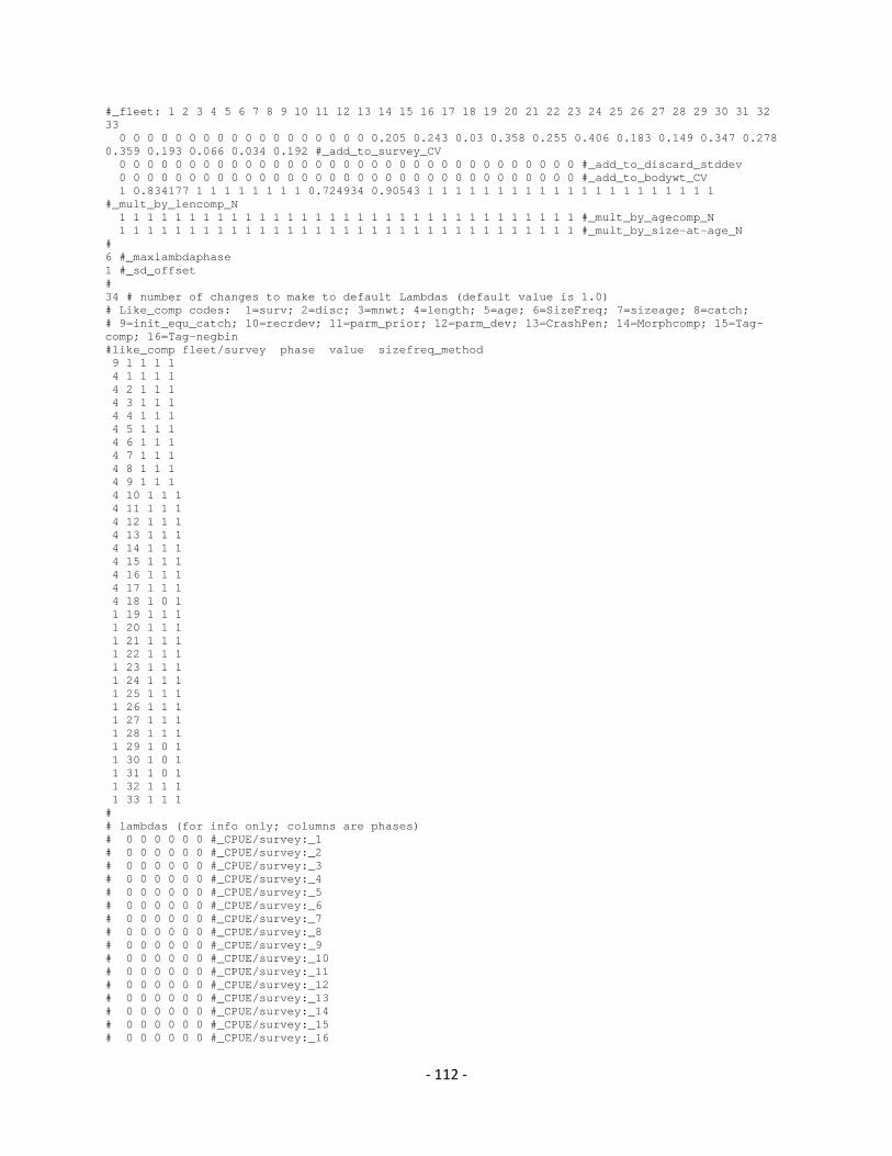
‐ 112 ‐

#_fleet: 1 2 3 4 5 6 7 8 9 10 11 12 13 14 15 16 17 18 19 20 21 22 23 24 25 26 27 28 29 30 31 32 33 0 0 0 0 0 0 0 0 0 0 0 0 0 0 0 0 0 0 0.205 0.243 0.03 0.358 0.255 0.406 0.183 0.149 0.347 0.278 0.359 0.193 0.066 0.034 0.192 #_add_to_survey_CV 0 0 0 0 0 0 0 0 0 0 0 0 0 0 0 0 0 0 0 0 0 0 0 0 0 0 0 0 0 0 0 0 0 #_add_to_discard_stddev 0 0 0 0 0 0 0 0 0 0 0 0 0 0 0 0 0 0 0 0 0 0 0 0 0 0 0 0 0 0 0 0 0 #_add_to_bodywt_CV 1 0.834177 1 1 1 1 1 1 1 1 0.724934 0.90543 1 1 1 1 1 1 1 1 1 1 1 1 1 1 1 1 1 1 1 1 1 #_mult_by_lencomp_N 1 1 1 1 1 1 1 1 1 1 1 1 1 1 1 1 1 1 1 1 1 1 1 1 1 1 1 1 1 1 1 1 1 #_mult_by_agecomp_N 1 1 1 1 1 1 1 1 1 1 1 1 1 1 1 1 1 1 1 1 1 1 1 1 1 1 1 1 1 1 1 1 1 #_mult_by_size-at-age_N # 6 #_maxlambdaphase 1 #_sd_offset # 34 # number of changes to make to default Lambdas (default value is 1.0) # Like_comp codes: 1=surv; 2=disc; 3=mnwt; 4=length; 5=age; 6=SizeFreq; 7=sizeage; 8=catch; # 9=init_equ_catch; 10=recrdev; 11=parm_prior; 12=parm_dev; 13=CrashPen; 14=Morphcomp; 15=Tag-comp; 16=Tag-negbin #like_comp fleet/survey phase value sizefreq_method 9 1 1 1 1 4 1 1 1 1 4 2 1 1 1 4 3 1 1 1 4 4 1 1 1 4 5 1 1 1 4 6 1 1 1 4 7 1 1 1 4 8 1 1 1 4 9 1 1 1 4 10 1 1 1 4 11 1 1 1 4 12 1 1 1 4 13 1 1 1 4 14 1 1 1 4 15 1 1 1 4 16 1 1 1 4 17 1 1 1 4 18 1 0 1 1 19 1 1 1 1 20 1 1 1 1 21 1 1 1 1 22 1 1 1 1 23 1 1 1 1 24 1 1 1 1 25 1 1 1 1 26 1 1 1 1 27 1 1 1 1 28 1 1 1 1 29 1 0 1 1 30 1 0 1 1 31 1 0 1 1 32 1 1 1 1 33 1 1 1 # # lambdas (for info only; columns are phases) # 0 0 0 0 0 0 #_CPUE/survey:_1 # 0 0 0 0 0 0 #_CPUE/survey:_2 # 0 0 0 0 0 0 #_CPUE/survey:_3 # 0 0 0 0 0 0 #_CPUE/survey:_4 # 0 0 0 0 0 0 #_CPUE/survey:_5 # 0 0 0 0 0 0 #_CPUE/survey:_6 # 0 0 0 0 0 0 #_CPUE/survey:_7 # 0 0 0 0 0 0 #_CPUE/survey:_8 # 0 0 0 0 0 0 #_CPUE/survey:_9 # 0 0 0 0 0 0 #_CPUE/survey:_10 # 0 0 0 0 0 0 #_CPUE/survey:_11 # 0 0 0 0 0 0 #_CPUE/survey:_12 # 0 0 0 0 0 0 #_CPUE/survey:_13 # 0 0 0 0 0 0 #_CPUE/survey:_14 # 0 0 0 0 0 0 #_CPUE/survey:_15 # 0 0 0 0 0 0 #_CPUE/survey:_16

‐ 113 ‐

# 0 0 0 0 0 0 #_CPUE/survey:_17 # 0 0 0 0 0 0 #_CPUE/survey:_18 # 1 1 1 1 1 1 #_CPUE/survey:_19 # 1 1 1 1 1 1 #_CPUE/survey:_20 # 1 1 1 1 1 1 #_CPUE/survey:_21 # 1 1 1 1 1 1 #_CPUE/survey:_22 # 1 1 1 1 1 1 #_CPUE/survey:_23 # 1 1 1 1 1 1 #_CPUE/survey:_24 # 1 1 1 1 1 1 #_CPUE/survey:_25 # 1 1 1 1 1 1 #_CPUE/survey:_26 # 1 1 1 1 1 1 #_CPUE/survey:_27 # 1 1 1 1 1 1 #_CPUE/survey:_28 # 0 0 0 0 0 0 #_CPUE/survey:_29 # 0 0 0 0 0 0 #_CPUE/survey:_30 # 0 0 0 0 0 0 #_CPUE/survey:_31 # 1 1 1 1 1 1 #_CPUE/survey:_32 # 1 1 1 1 1 1 #_CPUE/survey:_33 # 1 1 1 1 1 1 #_lencomp:_1 # 1 1 1 1 1 1 #_lencomp:_2 # 1 1 1 1 1 1 #_lencomp:_3 # 1 1 1 1 1 1 #_lencomp:_4 # 1 1 1 1 1 1 #_lencomp:_5 # 0 0 0 0 0 0 #_lencomp:_6 # 0 0 0 0 0 0 #_lencomp:_7 # 0 0 0 0 0 0 #_lencomp:_8 # 0 0 0 0 0 0 #_lencomp:_9 # 0 0 0 0 0 0 #_lencomp:_10 # 1 1 1 1 1 1 #_lencomp:_11 # 1 1 1 1 1 1 #_lencomp:_12 # 1 1 1 1 1 1 #_lencomp:_13 # 0 0 0 0 0 0 #_lencomp:_14 # 0 0 0 0 0 0 #_lencomp:_15 # 1 1 1 1 1 1 #_lencomp:_16 # 1 1 1 1 1 1 #_lencomp:_17 # 0 0 0 0 0 0 #_lencomp:_18 # 0 0 0 0 0 0 #_lencomp:_19 # 0 0 0 0 0 0 #_lencomp:_20 # 0 0 0 0 0 0 #_lencomp:_21 # 0 0 0 0 0 0 #_lencomp:_22 # 0 0 0 0 0 0 #_lencomp:_23 # 0 0 0 0 0 0 #_lencomp:_24 # 0 0 0 0 0 0 #_lencomp:_25 # 0 0 0 0 0 0 #_lencomp:_26 # 0 0 0 0 0 0 #_lencomp:_27 # 0 0 0 0 0 0 #_lencomp:_28 # 0 0 0 0 0 0 #_lencomp:_29 # 0 0 0 0 0 0 #_lencomp:_30 # 0 0 0 0 0 0 #_lencomp:_31 # 0 0 0 0 0 0 #_lencomp:_32 # 0 0 0 0 0 0 #_lencomp:_33 # 1 1 1 1 1 1 #_init_equ_catch # 1 1 1 1 1 1 #_recruitments # 1 1 1 1 1 1 #_parameter-priors # 1 1 1 1 1 1 #_parameter-dev-vectors # 1 1 1 1 1 1 #_crashPenLambda 0 # (0/1) read specs for more stddev reporting # 0 1 -1 5 1 5 1 -1 5 # placeholder for selex type, len/age, year, N selex bins, Growth pattern, N growth ages, NatAge_area(-1 for all), NatAge_yr, N Natages # placeholder for vector of selex bins to be reported # placeholder for vector of growth ages to be reported # placeholder for vector of NatAges ages to be reported 999

‐ 114 ‐

Appendix B Input file (REBUILD.DAT) for Rebuilder version 3.12b. Exampled model was based on re‐sampling recruitment for 1994‐2008 using current (2007‐2009) harvest rate (constant %). #Title SM 2011 # Number of sexes 1 # Age range to consider 0 15 # Number of fleets 3 # First year of projection (Yinit) 2010 # First year the oY could have been zero 2010 # Number of simulations 4000 # Maximum number of years 200 # Conduct projections with multiple starting values (0=No;else yes) 1 # Number of parameter vectors 100 # Is the maximum age a plus-group (1=Yes;2=No) 1 # Generate future recruitments using historical recruitments (1) historical recruits/spawner (2) or a stock-recruitment (3) 1 # Constant fishing mortality (1) or constant Catch (2) 1 # Fishing mortality based on SPR (1) or F (2) 1 # Pre-specify the year of recovery (or -1) to ignore -1 # Fecundity-at-age # 0 1 2 3 4 5 6 7 8 9 10 11 12 13 14 15 0 1.16 5.52 14.63 27 40.15 52.36 62.9 71.65 78.76 84.47 89.01 92.62 95.47 97.71 101.165 # Age specific information (females then males) weight / selectivity # wt and selex for "gender, fleet:" 1 1 18.138 30.132 40.759 49.969 57.554 63.668 68.579 72.523 75.687 78.221 80.244 81.855 83.135 84.151 85.716 85.716 0.082 0.539 0.864 1.000 0.908 0.724 0.552 0.425 0.339 0.282 0.245 0.220 0.203 0.191 0.182 0.171 # wt and selex for "gender, fleet:" 1 2 22.916 33.952 41.905 49.277 56.128 62.255 67.551 72.019 75.726 78.764 81.230 83.218 84.812 86.085 88.063 88.063 0.000 0.311 0.730 0.987 1.000 0.902 0.790 0.699 0.631 0.582 0.548 0.523 0.505 0.492 0.482 0.468 # wt and selex for "gender, fleet:" 1 3 3.508 35.398 46.314 55.562 64.246 72.434 79.908 86.496 92.137 96.864 100.761 103.935 106.497 108.552 110.191 112.774 0.000 0.143 0.464 0.718 0.855 0.921 0.955 0.972 0.983 0.989 0.993 0.995 0.997 0.998 0.999 1.000 # M and current age-structure # 0.505 0.45 0.415 0.39 0.38 0.38 0.38 0.38 0.38 0.38 0.38 0.38 0.38 0.38 0.38 0.38 325.741 195.288 33.3391 17.0388 3.20836 3.7906 0.388353 0.514413 0.315897 0.0688192 0.0348344 0.00581874 0.00123893 0.000539158 7.09607E-05 4.26994E-05 # Age-structure at the start of year Yinit 325.741 195.288 33.3391 17.0388 3.20836 3.7906 0.388353 0.514413 0.315897 0.0688192 0.0348344 0.00581874 0.00123893 0.000539158 7.09607E-05 4.26994E-05 # Year Ynit^0 2010 # recruitment and biomass # Number of historical assessment years 37 # Historical data # year recruitment spawner in B0 in R project in R/S project

‐ 115 ‐

1974 1975 1976 1977 1978 1979 1980 1981 1982 1983 1984 1985 1986 1987 1988 1989 1990 1991 1992 1993 1994 1995 1996 1997 1998 1999 2000 2001 2002 2003 2004 2005 2006 2007 2008 2009 2010 553.587 437.619 495.212 273.226 1341.2 371.167 598.323 552.392 225.432 431.128 1620.01 227.933 384.917 850.16 587.473 315.874 918.588 235.848 730.792 116.484 522.354 310.626 297.155 560.111 283.161 285.668 448.599 296.043 530.666 366.455 115.912 434.196 125.377 203.907 133.143 348.68 325.741 18480.35551 5261.380563 4128.805075 3686.649436 2722.718081 2043.020893 3004.158281 3538.663066 3437.225006 3474.213756 2809.672595 2887.839776 3676.045136 3726.565643 3079.070088 2937.42805 2972.531297 3040.115075 3178.396067 3079.507117 2750.813391 2158.828683 1437.121074 1204.071824 1146.902924 1134.50934 960.7501858 985.0652582 1169.504248 1418.171721 1886.872212 2064.654692 2037.92472 1870.837326 1579.37126 1088.321873 983.0446912 1 0 0 0 0 0 0 0 0 0 0 0 0 0 0 0 0 0 0 0 0 0 0 0 0 0 0 0 0 0 0 0 0 0 0 0 0 0 0 0 0 0 0 0 0 0 0 0 0 0 0 0 0 0 0 0 0 1 1 1 1 1 1 1 1 1 1 1 1 1 1 1 0 0 0 0 0 0 0 0 0 0 0 0 0 0 0 0 0 0 0 0 0 0 0 0 0 0 0 0 0 0 0 0 0 0 0 0 0 0 0 # Number of years with pre-specified catches # catches for years with pre-specified catches # Number of future recruitments to override 0 # Process for overiding (-1 for average otherwise index in data list) # Which probability to product detailed results for (1=0.5; 2=0.6; etc.) 8 # Steepness sigma-R, and auto-correlation 0.87 0.62 0 # Target SPR rate (FMSY Proxy) 0.178 # Discount rate (for cumulative catch) 0.1 # Truncate the series when 0.4B0 is reached (1=Yes) 0 # Set F to FMSY once 0.4B0 is reached (1=Yes) 0 # Maximum possible F for projection (-1 to set to FMSY) -1 # Definition of recovery (1=now only;2=now or before) 1 # Projection type (1, 2, 3, 4, 5, 11 or 12) 11 "# Definition of the ""40-10"" rule" .01 .02 # Calculate coefficients of variation (1=Yes) 0 # Number of replicates to use 10 # Random number seed -99004 # File with multiple parameter vectors Marlin.dat # User-specific projection (1=Yes); Output replaced (1->9) 1 8 # Catches and Fs (Year; 1/2 (F or C); value); Final row is -1 2010 1 1.0718 2011 1 1.0718 2012 3 0.14 2013 3 0.14 2014 3 0.14 -1 -1 -1 # Fixed catch project (1=Yes); Output replaced (1->9); Approach (-1=Read in else 1-9) 0 2 -1 # Split of Fs 2010 0.13 0.48 0.39 2011 0.13 0.48 0.39 2012 0.13 0.48 0.39 -1 -1 -1 -1 # Five pre-specified inputs .12 .14 .2 .25 .3 # Years for which a probability of recovery is needed 2013 2014 2015 2016 2017 2018 2019 2020 # Time varying weight-at-age (1=Yes;0=No) 0

‐ 116 ‐

# File with time series of weight-at-age data none # Use bisection (0) or linear interpolation (1) 0 # Target Depletion 0.147 # CV of implementation error 0

Documents

CENTRAL NORTH PACIFIC OCEAN - National …€ 2 ‐ 4.5 Observation models for the data 27 4.5.1 What CPUE indices should be included 27 4.5.2 Weighting of model